PROCEEDINGS, 43rd Workshop on Geothermal Reservoir Engineering
Stanford University, Stanford, California, February 12-14, 2018
SGP-TR-213
1
DAS and DTS at Brady Hot Springs: Observations about Coupling and Coupled
Interpretations
Douglas E. Miller
Earth Resources Laboratory, Department of Earth, Atmospheric and Planetary Sciences, Massachusetts Institute of Technology, 1215
77 Massachusetts Avenue, Cambridge MA 02139 United States
Thomas COLEMAN(3), Xiangfang ZENG(1,9), Jeremy R. PATTERSON (1), Elena C. REINISCH(1), Michael A.
CARDIFF(1), Herbert F. WANG(1), Dante FRATTA(1), Whitney TRAINOR-GUITTON(7), Clifford H. THURBER(1),
Michelle ROBERTSON(2), Kurt FEIGL(1), and The PoroTomo Team(1-9)
(1) University of Wisconsin-Madison, Department of Geoscience, Madison, WI, United States;
(2) Lawrence Berkeley National Laboratory, Berkeley, CA, United States;
(3) Silixa LLC, Houston, TX, United States;
(4) Ormat Technologies Inc., Reno, NV, United States;
(5) University of Nevada Reno, NV, United States;
(6) Lawrence Livermore National Laboratory, Livermore, CA, United States;
(7) Colorado School of Mines, Golden, CO, United States;
(8) Temple University, Philadelphia, PA, United States;
(9) State Key Laboratory of Geodesy and Earth's Dynamics,Institute of Geodesy and Geophysics, Chinese Academy of Sciences
http://geoscience.wisc.edu/feigl/porotomo/
Keywords: EGS, DAS, DTS
ABSTRACT
In March 2016 an extensive integrated survey was performed at the geothermal field at Brady Hot Springs, Nevada, where highly
permeable conduits along faults appear to channel fluids from shallow aquifers to the deep geothermal reservoir tapped by the
production wells. The data set included two fiber-optic cable Distributed Acoustic Sensing (DAS) and Distributed Temperature Sensing
(DTS) systems. One cable was arranged horizontally in a zigzag trench 8700 m in length. The second cable was deployed into the
accessible 363m portion of a vertical well near another monitoring well. Both cables contained both single-mode and multi-mode fibers
with optical U-bends at the ends. Silixa DTS and DAS interrogators were operated to continuously monitor the trenched cable (DASH
and DTSH) for 15 days and the borehole cable (DASV and DTSV) for 8 days. In addition to providing active and passive seismic
waveform data, the DAS was processed to extract fiber slow strain at a rate comparable to the DTS (2 samples/min).
Combined analysis of both DAS and DTS in both horizontal and vertical deployments show details, including puzzling observations,
where the combined datasets help to identify and interpret anomalous coupling of the fiber measurements to environmental signal.
Patterns in DTSH response as a function of both time and position document thermal response to daily temperature cycles and to
changes in injection and production pressure. A magnitude 4.3 regional earthquake from a source in Hawthorne NV, 100 km south of
Brady, was clearly detectable by both DASH and DASV. Comparison with Nodal geophones confirmed and cross-calibrated the
instrument response of each system. Local earthquakes detectable by the DASH installation include all of those catalogued by the local
LBL Brady seismic array plus several additional events of likely interest.
Slow strain measured by the DASV is highly correlated to temperature change measured by DTSV. Synchronous patterns in DASV and
DTSV document repetitive cycles of thermal exchange both at the expected fluid level in the well and at the level of the slotted liner.
DASV documents resonant acoustic behavior associated with the process. Events in DASV data suggest that thermal reaction to
borehole rewarming periodically breaks the frictional coupling between cable and borehole wall causing slippage. Patterns in the DASV
and DTSV data suggest that the upper section of casing is backed by a fluid annulus that is hydraulically connected to the main bore.
Low-frequency (6.4 Hz) resonant pressure transients detected by the DASV at the slotted liner correlate to quasi-periodic (semihourly)
thermal events at the same location detected by the DTSV array. Both the earthquake arrival and VSP waveforms extracted from the
DASV active-source recordings show a vertical compressional propagation velocity close to 2 km/sec.
1. INTRODUCTION
In March 2016 an extensive integrated survey was performed at the geothermal field at Brady Hot Springs, Nevada, where highly
permeable conduits along faults appear to channel fluids from shallow aquifers to the deep geothermal reservoir tapped by the
production wells.
The 15-day deployment included 4 distinct stages with intentional manipulations of the pumping rates in injection and production wells.
The deployment included fiber-optic cables for Distributed Acoustic Sensing (DAS) and Distributed Temperature Sensing (DTS)
arranged vertically in a borehole to ~400 m depth and horizontally in a trench 8700 m in length.

Miller, Coleman and PoroTomo team
2
Because the DAS and DTS fibers were collocated in common cables, the data are rich in observables that can guide and constrain
interpretation of each measurement, particularly at locations and times where there are discontinuities in the coupling of the cables to
the environment or where heterogeneous environmental processes occur.
Previous publications, including papers at the 2017 Stanford Geophysical Workshop, have described the overall context of the surveys
and discussed preliminary analysis. It is a goal of this paper to highlight some details, including puzzling observations, where the
combined observations help to identify and interpret anomalous coupling of the fiber measurements to environmental signal.
Metadata describing each of these data sets are available at the Geothermal Data Repository (GDR):
https://gdr.openei.org/search?q=porotomo&submit=Search. All of the data became available to the public on October 1st, 2017 at
ftp://roftp.ssec.wisc.edu/porotomo.
2. DAS AND DTS MEASUREMENT PRINCIPLES
DTS and DAS are based on optical time domain reflectometry (OTDR) measurement techniques in which an incident pulse of light is
coupled into an optical fiber and backscattered light sampled. As the incident pulse travels along the fiber, at each sampling interval of
fiber, a small amount of light is scattered and recaptured by the fiber waveguide in the return direction. Local variations of the
backscatter waveform provide information on the state of the fiber at successive sampling intervals determined by the roundtrip transit
time from launching end to point of interest. Through continuous analyses of the backscattered signal from successive incident pulses,
dynamic profiles of both temperature and acoustics (dynamic strain) are realized as a continuous 2D function of recording time and
distance along the fiber. The principles of DAS and DTS are discussed in the published literature (e.g. Parker et al. 2014, Daley et al.
2015, and Dakin et al. 1985). The DTS data delivered to the PoroTomo project were collected using an ULTIMA-STM DTS with a
double-ended configuration that utilizes a loop of optical fiber and had spatial sampling intervals of 0.126 m. Silixa’s iDASTM was
utilized for DAS acquisition with channel spacing of 1.021 m and a gauge length of 10 m.
Data delivered to the PoroTomo project (and stored in the public archive) was in the form of .sgy files with raw units (radians of optical
phase change per time sample). As described e.g. in Daley et al. (2015), Miller et al. (2016) and Wang et al. (2017), iDAS data can be
rescaled to fiber strain scaling by nanometers of elongation per radian per gauge length per timestep (i.e., by 11.6) and then by
integrating with respect to time. Data shown herein had those steps applied as well as a step to estimate and remove a common nuisance
signal. The nuisance signal stems from a small sensitivity to vibration of the interrogator and is uniformly present on all channels and is
therefore perfectly aligned across all channels.
DAS slow strain
Provided recordings are continuous and contiguous, DAS data can be averaged to provide a very narrow temporal bandwidth estimate of
fiber response. The files below that are labeled “slow strain” have been created with values denominated in microstrain per minute by
summing 30-second strain rate files over all timesamples and doubling the resulting values. This is effectively a lowpass filter followed
by a resampling.
Fiber particle velocity from DAS
DAS fiber strain signals can be converted to fiber particle velocity by an appropriate additional step in the process chain. In
mathematical terms, following Daley et al. (2015) and Wang et al. (2017) write u(z,t) for the displacement (with respect to an arbitrary
initial position) of the fiber at spatial location z and recording time t. The signal s(z,t) is proportional to a spatially averaged finite-
difference approximation to the mixed derivative
(1)
Here, * represents convolution and A(z) represents the intensity profile of the propagating probe light pulse within the fiber. Equation
(1) may equivalently be regarded as a spatial derivative of the fiber particle velocity v = u/t or as a temporal derivative of fiber strain
= u/z. Writing U(k, ), S(k, ) and A(k) for the 2D Fourier transforms of u, and s, and A respectively,
S(k, ) = k U(k, ) A(k) (2)
hence, writing E and V for the 2D Fourier transforms of (spatially averaged) fiber strain and particle velocity,
/k E(k) = 1/k S(k,) = U(k) = V(k,) (3)
The equivalence of the first and last terms in (3) expresses the fact suggested by Daley et al. (2015) that the fiber particle velocity can be
recovered as the inverse 2D Fourier transform of fiber strain after rescaling pointwise in the transform domain by phase speed 𝑐=𝜔/k.
This equation is the basis for numerical implementation used to process the Brady field data displayed here.

Miller, Coleman and PoroTomo team
3
3. DAS AND DTS RECORDINGS AT BRADY
3.1 Installation
Two interrogators of each type were used at Brady. Figure 1 (left) shows the four units in the recording shed labeled by function (DTS
or DAS) and disposition of the optical cable (vertical in well 56-1 or horizontal in the zigzag trench) to which each is connected; (right)
shows photos of the trench and wellhead with schematics of the corresponding cables. The inset (Feigl et al. (2018) Figure 5) shows the
layout of the trench and the location of the 56-1 wellhead. The recording shed was at the end of the trench closest to the wellhead. The
arrows in the middle-bottom photo are pointing to an electrical connection. The actual fiber connection box was at the opposite end of
the recording shed and is not seen in the photo.
Figure 1. Photos of interrogators (left) and cable installation (right).
Typical optical cables contain several bundled fibers within outer protective layers. Two types of cable were used at Brady. The
trenched cable was a tight-buffered construction with a polymer jacket, the borehole cable was a fiber in metal tube (FIMT) based
construction. Each cable contained several of both types of fiber: multimode (MM), used for DTS, and singlemode (SM), used for DAS.
For each installation a pair of MM fibers were joined at the far end with a u-bend termination to allow a double-ended DTS
configuration. The upper right photo in Figure 1 shows the splicebox at the terminus of the trench. A similar spliced pair of SM fibers
were used for the borehole DAS installation (DASV) which was recorded over an interval that included both the wellhead and the
turnaround splice with about 10 extra channels at each end (an aid to matching DTS and DAS channels with well geometry).
3.2 Trenched Cable Recordings
The trenched cable was an 8.7 km zigzag in 71 segments. Segments 1 through 29 were outbound from the recording shed roughly
parallel to eastbound I-80. Segments 301 through 49 ran inbound, crossing the service road at segment 47. Segments 50 through 71
were outbound south of the service road (visible in the Google Earth underlay in Figure 2).
DTSH
Figure 2 shows DTS recordings from the trenched cable. The left panel shows a planview of the survey area with DTSH and DASH
slow strain overlain as a ribbon on top of a Google Earth image annotated with fumarole and “warm ground” locations. The lower right
panel shows data for the entire two-week period March 12 to 26 for the segments that constitute the first outgoing (1:29) portion of the
installation. The two lower panels show the ingoing (30:49) and final outgoing (50:71) portion. Segment numbers on the left mark the
starts of the corresponding segments. The panel at top right shows the pressure recorded in the two monitor wells displayed as variation
in hydrostatic head (in mH2O) from their initial values. The vertical red lines on the right panels indicate the time, 20-Mar 12:05 (UTC),
corresponding to the overlay on the left. Note that segment 1 is short. The 56-1 borehole is between segments 3 and 5.
Several features are easily seen in the display. There are several locations (marked S) where optical splices in spliceboxes, similar to the
one shown in Figure 1, were left exposed to the air. All of the cable in segments 42 (close to the service road) and 47 (in a culvert
crossing the road) were also exposed. Those channels clearly register the air temperature. Segment 42 in the lower left panel is the
easiest place to see this. During the survey period, local time was MDT, 6 hours behind UTC. Local sunrise was at about 7am local time
so 12:00 UTC was typically the coldest part of each day. Each day’s dawn can be recognized as the point where segment 42 turns from
blue to brown in the display.
Unsurprisingly, the channels closest to the fumaroles are the warmest in general but certain locations are identifiable in Figures 2 and 5
as local hot spots. Segments 53:71 are consistently cooler than others. Note that all segments show response to the changes in pumping
stages, most notably to the increased injection stage March 18-24. There is also evident diurnal variation that varies with location but is
typically almost 180 degrees (12 hours) out of phase with the air temperature. The ground is warmest when the air is coldest. Segments
17:22 are particularly interesting in this regard. Perhaps this can be analyzed in terms of heat flow in response to the changing surface
boundary condition and associated increase in temperature gradient. The cable was buried at approximately 1 m depth with unmeasured
precision using a Ditch Witch trencher to cut the trench.

Miller, Coleman and PoroTomo team
4
Figure 2. DTS recordings from the trenched cable
DASH
Because a magnitude 4.3 earthquake occurred near Hawthorne, Nevada, about 100 km south of Brady, at 21-March-2016 07:37:10, it is
natural to use the arrival from that earthquake arrival both to illustrate key steps in the DAS processing and to compare DAS with nodal
geophones. The vector from the source location to Brady is nearly aligned with segment 52.
Figure 3 shows DASH fiber particle velocity for all channels for 30 seconds that include the main P and S arrivals at 07:37:37.5 (UTC)
and 07:37:57.5 (UTC) respectively. Note that the rescaling from fiber strain to fiber particle velocity changes the relative amplitudes of
coherent signals with distinct apparent velocities and thereby reduces the relative amplitude of the local environmental nuisance signal
propagating as surface waves. Note also the flip in polarity of coherent events at segments 30 and 50 where the fiber switches between
outbound and inbound sections, hence switching the sign of apparent velocity.
Miller, Coleman and PoroTomo team
5
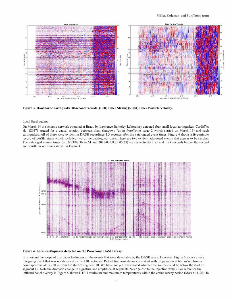
Figure 3. Hawthorne earthquake 30-second records. (Left) Fiber Strain; (Right) Fiber Particle Velocity.
Local Earthquakes
On March 14 the seismic network operated at Brady by Lawrence Berkeley Laboratory detected four small local earthquakes. Cardiff et
al. (2017) argued for a causal relation between plant shutdown (as in PoroTomo stage 2 which started on March 13) and such
earthquakes. All of these were evident in DASH recordings 1.3 seconds after the catalogued event times. Figure 4 shows a five-minute
record of DASH strain which included two of the catalogued times. There are two evident additional events that appear to be similar.
The cataloged source times (2016/03/08:36:26.61 and 2016/03/08:39:05.23) are respectively 1.81 and 1.28 seconds before the second
and fourth picked times shown in Figure 4.
Figure 4. Local earthquakes detected on the PoroTomo DASH array.
It is beyond the scope of this paper to discuss all the events that were detectable by the DASH array. However, Figure 5 shows a very
intriguing event that was not detected by the LBL network. Picked first arrivals are consistent with propagation at 600 m/sec from a
point approximately 250 m from the start of segment 10. We have not yet investigated whether the source could be below the start of
segment 10. Note the dramatic change in signature and amplitude at segments 24:42 (close to the injection wells). For reference the
lefthand panel overlay in Figure 5 shows DTSH minimum and maximum temperatures within the entire survey period (March 11-26). In

Miller, Coleman and PoroTomo team
6
that display, the splicepoints, exposed segments, and local hotspots are identifiable. The red circles on the left panel correspond to the
tickmarks on the right panel. The right panel shows trace-normalized fiber strain rate.
Figure 5. Mystery event at 08:32:06 (UTC) on March 15.
DAS and Geophone comparison
At Brady 240 3-component nodal geophone units were installed at ground level. To good approximation, for a geophone the raw
measurement (typically in millivolts generated by relative motion of a magnet and coil) is directly proportional to the velocity difference
between a proof mass and its housing. The geophone proof mass is coupled to the geophone housing by a weak spring. At temporal
frequencies well-above the resonant frequency of the spring-mass system, the housing moves while inertia keeps the proof mass still and
the relative motion is nearly identical to the ground motion at the location of the sensor. As described in Shearer (2009) (Section 11.1),
at lower frequencies the housing motion (and if the coupling is perfect, the local earth motion) can be recovered from the relative
motion by a simple equation (e.g. Shearer (2009) Equation 11.2). In the temporal frequency band of the Hawthorne earthquake
(centered at 2 Hz), the 5 Hz Nodal geophones are effectively behaving as accelerometers.
Figure 6. Comparison of DAS fiber velocity with ground motion estimated from horizontal geophones. Red circles in the inset
mark the geophone locationa at nodal stations 150 (left) and 48 (right).
Figure 6 compares the component of ground velocity parallel to the cable recovered from horizontal geophones using nominal values
for geophone sensitivity and response function to DAS fiber particle velocity near the geophones for two representative locations. The
match is not perfect, but it is typical of what we found. It is reassuring that no data-adaptive parameters (other than the uniform
bandpass applied to both) were used for either measurement. Note that geophone measurement is intrinsically local to the place where

Miller, Coleman and PoroTomo team
7
the geophone is installed (i.e. it is a point sensor) and, for heterogeneous media responding to coherent signal, its response may not be a
perfect representation of the average particle velocity response within a seismic wavelength. Similar comparisons made using slightly
different approach to process workflow are documented in Wang et al. (2017).
3.3 Borehole Cable Recordings
The vertical installation in well 56-1 was organized quickly after an initial deployment in well 55-1 failed when an in-well calcification
collapsed under the weight of sand which was intended to improve coupling between the fiber cable and borehole wall. Well 56-1 was
drilled to 725 m in 1991. The schematic well construction drawing shown in Figure 7 appears to be referenced to Ground Level and
shows cemented 17 inch production casing to 302 m and a slotted liner between 296 m and 363 m. The bottom of 20 inch outer casing
is shown at 285 ft (GL) = 87 m.
Figure 7. 56-1 completion geometry (left), cable description (lower right) and early DTSV record (upper right).
369 m of 3.2 mm (1/8 in) optical fiber in double metal tube (FIMT) cable was deployed into the well. It contained both single-mode and
multi-mode fibers with optical U-bends at the bottom. The DTSV record shown in Figure 7 identifies the start of spooled surface cable
at 273 m, the splice between surface and metal-tube cable at 504 m, the well-entry at 514 m and the fiber U-bend at 881 m.
DTSV Observations
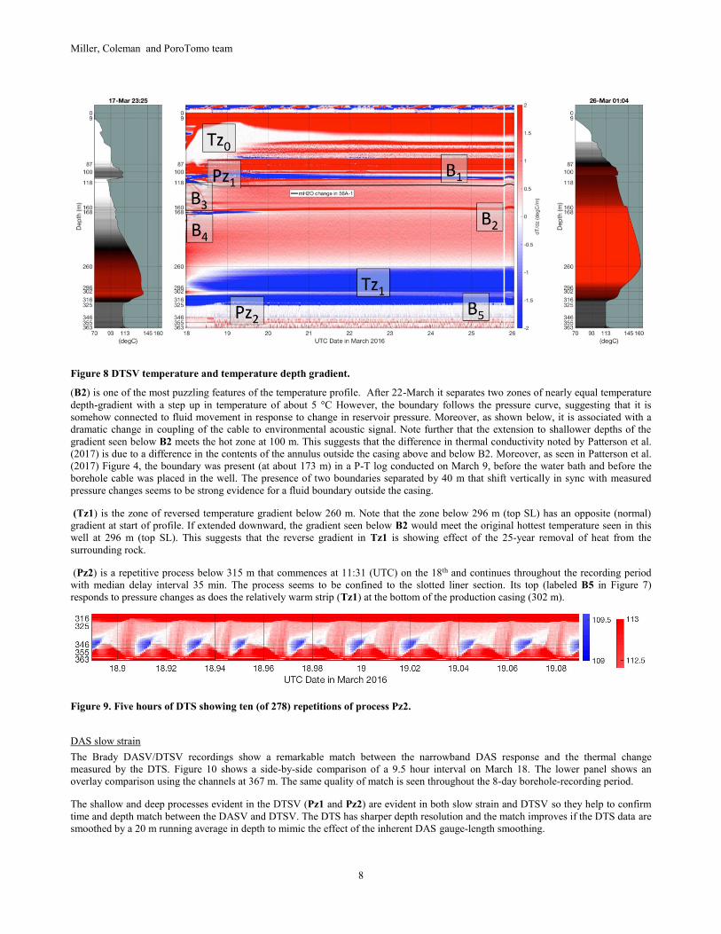
DTSV data are rich in observable phenomena (e.g. Patterson et al. (2017), Patterson et al. (2018)). The left and right panels of Figure 8
show temperature profiles from the first and last DTSV recordings, 17-Mar 23:25 (UTC) and 26-Mar 01:04 (UTC), respectively. The
center panel shows the vertical temperature gradient in °C/m for the entire eight day recording period.
Various evident zones, boundaries, and active thermal processes have been labeled. As a visual reference, the downhole pressure
recorded in the nearby well 51A-1 has been converted to meters of water and displayed as a black overlay curve at an arbitrary depth
near 120 m. Pressure increases upward in the display. The original recording in 56A-1 was made at a fixed depth so the shape of the
curve is proportional to water level in 56A-1 as a function of UTC date.
Process (P0) above the wellhead (-12 to 0 m) is the daily atmospheric cycle detected by portions of the cable outside the wellhead.
Process (Pz1) between 77 m and 120 m is a process that has been interpreted by Patterson et al. (2017) as boiling at the top of the fluid
in the borehole in response to pressure change. Pz1 commences at 14:09 (UTC) on March 18 and subsequently expands and then
contracts in depth, with delay intervals roughly decreasing from 30 min to 10 min. The process dies out on March 19 leaving a clear
thermal discontinuity at its lower boundary (B1). Note that B1 depth follows the pressure curve – most dramatically when pressure
increases during the site shutdown on March 25. Note further that the shallower boundaries, including the top and bottom of Tz0 do not
follow the pressure curve. Zone (Tz0) is a patch defined by a uniform temperature of 93 °C and a shape that appears to be related to the
shape of Pz1. Initially it is based at the level of the bottom of outer casing (87 m).
Miller, Coleman and PoroTomo team
8
Figure 8 DTSV temperature and temperature depth gradient.
(B2) is one of the most puzzling features of the temperature profile. After 22-March it separates two zones of nearly equal temperature
depth-gradient with a step up in temperature of about 5 °C However, the boundary follows the pressure curve, suggesting that it is
somehow connected to fluid movement in response to change in reservoir pressure. Moreover, as shown below, it is associated with a
dramatic change in coupling of the cable to environmental acoustic signal. Note further that the extension to shallower depths of the
gradient seen below B2 meets the hot zone at 100 m. This suggests that the difference in thermal conductivity noted by Patterson et al.
(2017) is due to a difference in the contents of the annulus outside the casing above and below B2. Moreover, as seen in Patterson et al.
(2017) Figure 4, the boundary was present (at about 173 m) in a P-T log conducted on March 9, before the water bath and before the
borehole cable was placed in the well. The presence of two boundaries separated by 40 m that shift vertically in sync with measured
pressure changes seems to be strong evidence for a fluid boundary outside the casing.
(Tz1) is the zone of reversed temperature gradient below 260 m. Note that the zone below 296 m (top SL) has an opposite (normal)
gradient at start of profile. If extended downward, the gradient seen below B2 would meet the original hottest temperature seen in this
well at 296 m (top SL). This suggests that the reverse gradient in Tz1 is showing effect of the 25-year removal of heat from the
surrounding rock.
(Pz2) is a repetitive process below 315 m that commences at 11:31 (UTC) on the 18th and continues throughout the recording period
with median delay interval 35 min. The process seems to be confined to the slotted liner section. Its top (labeled B5 in Figure 7)
responds to pressure changes as does the relatively warm strip (Tz1) at the bottom of the production casing (302 m).
Figure 9. Five hours of DTS showing ten (of 278) repetitions of process Pz2.
DAS slow strain
The Brady DASV/DTSV recordings show a remarkable match between the narrowband DAS response and the thermal change
measured by the DTS. Figure 10 shows a side-by-side comparison of a 9.5 hour interval on March 18. The lower panel shows an
overlay comparison using the channels at 367 m. The same quality of match is seen throughout the 8-day borehole-recording period.
The shallow and deep processes evident in the DTSV (Pz1 and Pz2) are evident in both slow strain and DTSV so they help to confirm
time and depth match between the DASV and DTSV. The DTS has sharper depth resolution and the match improves if the DTS data are
smoothed by a 20 m running average in depth to mimic the effect of the inherent DAS gauge-length smoothing.

Miller, Coleman and PoroTomo team
9
Figure 10. Narrowband DAS and DTS Comparison
The match between slow strain and DTS temperature change is obtained with a scaling coefficient of .2 microstrain per °C. Evidently
the narrowband DAS response is a thermal effect, but the proportionality factor provides a challenge/opportunity for explanation. It is
known (e.g. Bakku (2015; Section 3.4, equation 3.11)) that the length measured by DAS is sensitive to changes in both local strain and
local refractive index. For seismic signals, bandlimited to above 1 Hz, the temperature change over the relevant time duration is
negligible. When data are integrated over periods of tens of seconds or longer, the sensitivity of refraction index (the thermo-optic
effect) can be significant. Published values for these sensitivities (Fang et al. (2012; Section 3.1.7), cited by Bakku (2015)), suggests
that the change in refractive index may be similar to the thermal expansion coefficients for steel. The combined effect for fiber in a steel
tube in a steel-cased borehole should give apparent change in strain due to temperature change of about 20 microstrain per °C. This
differs from the Brady coefficient by a factor of 100. The combination of the significant detailed match between DAS and DTS signals
and significant mismatch between the calibration coefficient and its theoretical value suggests that the details of the steel cable’s design
may be important. The change in physical length should be a combination of the expansion/contraction of the acrylate coated glass fiber
directly and the effect from some unknown strain transfer function to the fiber (in a FIMT) from the composite of surrounding material
properties. If the steel tube of the cable expands uniformly (both circumferentially and axially), the resulting volume increase could
cause a net contracting force applied to the fibers inside. There would be clear benefit from a lab study testing to characterize the
variance between different fiber designs.
In the context of hydrofracture monitoring, Karrenbach et al. (2017a; Figure 14) showed a somewhat similar example where integrated
(narrow-bandwidth) DAS was scaled to provide a match to temperature change measured by a collocated DTS fiber. The scaling
coefficient was not reported.
DASV signal from repetitive borehole processes
Figure 11 shows a typical slip event seen on slow strain (left) and raw DASV strain rate (right). Note that the right panel shows a half-
second of recording time and is denominated in radians per msec. It shows that the slip event starts at 260 m depth and propagates as a
rupture. Note further that the interval between 9 m and 160 m shows a reverberation that starts at about 90 m, 25.6 sec. This
reverberation is typical of what is seen at all times in the DASV data. The propagation speed for the reverberation (4.6 km/sec) is typical
for extensional vibration in steel. Since both the cable sheath and the casing are steel, this observation does not resolve the question of

Miller, Coleman and PoroTomo team
10
whether the undamped interval is essentially due to lack of contact between cable and casing or lack of contact between casing and rock.
However the coincident thermal effect and especially the observation discussed above, that the lower boundary of this interval was
present as a thermal discontinuity before the cable was installed, argue strongly that the casing is ringing.
Figure 11. Typical slip event seen on slow strain (left) and raw DASV (right);
Some relatively rapid vibration is evident below 346 m in the right panel of Figure 11. Figure 12 documents that such vibration is
regularly detectable as a feature of the deep process. Five hours of measurements are shown. The lower panel shows slow strain (blue)
and broadband strain rate (brown) at 346 m depth. Upper panel shows temporal spectrum of the brown curve. It seems possible that the
borehole is acting as a Helmholtz resonator or very long organ pipe driven by flow through the perforated liner.
Figure 12. Five hours of resonant behavior associated with the deep process. Lower panel shows slow strain (blue) and
broadband strain rate (brown). Upper panel shows temporal spectrum of the brown curve.
DASV seismic response
Figure 13 shows DASV for a 10-sec. interval containing the first arrival of the Hawthorne earthquake on March 21. The vertical axis is
denoted in channels and includes the turnaround at channel 372 (= 363 m). The wellhead entry is at channel 7. Note that the coherent

Miller, Coleman and PoroTomo team
11
signal is clear in and only in the interval from 160 m to 300 m. The apparent velocity (2 km/sec) is consistent with propagation seen in
near-offset active-source (Vibe) recordings. The ringing in the shallow zone is similar to the ringing seen in Figure 12 and all other
DASV recordings.
Figure 13. Hawthorne earthquake arrival on DASV.
Figure 14. Processed Vibe data from two shotpoints annotated with traveltimes calculated in a 1D model.

Miller, Coleman and PoroTomo team
12
DASV traveltimes
The task of reconciling DASV active-source recordings with tomographic inversions based on the surface recordings (e.g. as shown in
Feigl et al. (2018), Thurber et al. (2017), Matzel et al. (2018), Zeng et al (2017), Trainor-Guiton (2018)) has been started but not yet
completed. Typical borehole seismic processing (e.g. Miller et al (2016)) starts with a one-dimensional layered model built to match
direct arrivals from near-offset sources and adjusts the model to match arrivals from other source locations. The simplest correction
involves treating variation as mainly due to source elevation and near-surface slow propagation by calculating a per-source time shift to
match modeled and measured arrival times. Figure 14 shows examples of this process applied to Brady DASV data. Waveforms shown
are the result of correlating the recorded source sweep with DASV strain and averaging over repeat sweeps at the same location. The
model P velocity was 1700 m/sec above 25 m, 2200 m/sec between 190 m and 220 m, 1800 m/sec elsewhere; S velocity was 40 m/sec
above 25 m, and 900 m/sec elsewhere. This P-velocity is significantly slower over this depth interval (150-300 m sub GL) than those
shown by Feigl et al. (2018). Note that refraction in a heterogeneous model can yield apparent velocity that is faster than true velocity
but not slower.
Each data panel is annotated with one cyan curve calculated traveltimes for direct (downgoing) P and two magenta curves showing the
calculated traveltimes for direct (downgoing) S as well as a PS reflection from an interface at 320 m. Shot positions are indicated by red
circles on the panels at top. Note that the coordinate system used in this figure is centered at the 56-1 wellhead and rotated about 90
degrees from that shown in other figures herein. Note that the PS reflection is strongly evident for SP 125 and absent for SP 199. It is
possible that the strong downgoing event that is about 100 msec after the indicated direct S is the “true” direct S and that the label
matches a downgoing shear converted at a near-vertical interface (fault or fracture) that more strongly affects SP 125 than SP 199.
CONCLUSIONS
Patterns in both DTSH and DASH show details of local ground heterogeneity and associated heterogeneity of DAS coupling and
seismic propagation.
Patterns in DTSH response as a function of both time and position document thermal response to daily temperature cycles and to
changes in injection and production pressure.
A magnitude 4 regional earthquake from a source in Hawthorne NV, 100 km south of Brady, was clearly detectable by both DASH and
DASV. Comparison with Nodal geophones confirmed and cross-calibrated the instrument response of each system.
Local earthquakes detectable by the DASH installation include all of those catalogued by the local LBL Brady seismic array plus
several additional events of likely interest.
Patterns in both DTSV and DASV suggest that the there may be a fluid boundary in the annulus outside the casing above 160 m.
Slow strain measured by the DASV is highly correlated to temperature change measured by DTSV and may be related to a combined
effect of the change in refractive index and elongation/contraction of the glass optical fiber and surrounding media
Synchronous patterns in DASV and DTSV document repetitive cycles of thermal exchange both at the expected fluid level in the well
and at the level of the slotted liner. DASV documents resonant acoustic behavior associated with the process.
Events in DAS data suggest that thermal reaction to borehole rewarming periodically breaks the frictional coupling between cable and
borehole wall causing slippage
Patterns in the DAS and DTS data suggest that the upper section of casing is backed by a fluid annulus that is hydraulically connected to
the main bore.
Low-frequency (6.4 Hz) resonant pressure transients detected by the DASV at the slotted liner correlate to quasi-periodic (semihourly)
thermal events at the same location detected by the DTSV.
Both the earthquake arrival and VSP waveforms extracted from the DASV active-source recordings show a vertical compressional
propagation velocity close to 2 km/sec.
ACKNOWLEDGMENTS
Elena C. Reinisch was supported by the National Science Foundation Graduate Research Fellowship under grant DGE-1256259. The
work presented herein was funded in part by the Office of Energy Efficiency and Renewable Energy (EERE), U.S. Department of
Energy, under Award Numbers DE-EE0006760 and DE-EE0005510. Further acknowledgments found in Feigl et al. (2018) are
incorporated here by reference.
REFERENCES
Bakku, S. K. (2015), Fracture characterization from seismic measurements in a borehole, Ph.D. thesis, 227 pp, Massachusetts Institute
of Technology.
Cardiff, M., D. Lim, J. Patterson, J. Akerley, P.Speielman, J. Lopeman, P. Walsh, A. Singh, W. Foxall, H. Wang, N. Lord, C. Thurber,
D. Fratta, R. Mellors, N. Davatzes, and K. Feigl (2017) Geothermal production and reduced seismicity: Correlation and proposed
mechanism. Earth and Planetary Science Letters 482, pp 470-477 https://doi.org/10.1016/j.epsl.2017.11.037

Miller, Coleman and PoroTomo team
13
Daley, T. M., D. E. Miller, K. Dodds, P. Cook, and B. M. Freifeld (2015), Field testing of modular borehole monitoring with
simultaneous distributed acoustic sensing and geophone vertical seismic profiles at Citronelle, Alabama, Geophysical Prospecting.
http://dx.doi.org/10.1111/1365-2478.12324
Fang, Z., K. Chin, R. Qu, H. Cai, H., and K. Chang (2012). Fundamentals of Optical Fiber Sensors (1st ed.). Hoboken, N.J: Wiley
Feigl, K. L., and PoroTomo_Team (2017), Overview and Preliminary Results from the PoroTomo Project at Brady Hot Springs,
Nevada: Poroelastic Tomography by Adjoint Inverse Modeling of Data from Seismology, Geodesy, and Hydrology, paper presented at
Stanford Geothermal Workshop, Stanford University. https://pangea.stanford.edu/ERE/db/GeoConf/papers/SGW/2017/Feigl.pdf
Karrenbach, M., A. Ridge, S. Cole, K. Boone, D. Kahn, J. Rich, K. Silver, and D. Langton (2017) DAS Microseismic Monitoring and
Integration With Strain Measurements in Hydraulic Fracture Profiling. Unconventional Resources Technology Conference, Austin,
Texas, 24-26 July 2017: pp. 1316-1330.
Matzel, E., C. Morency, and D. Templeton (2018), Measuring the Material Properties Beneath Geothermal Fields Using Interferometry,
paper presented at PROCEEDINGS, 43rd Workshop on Geothermal Reservoir Engineering, Stanford University, Stanford, California,
February 12-14, 2018.
Miller, D. E., T. Daley, D. White, B. Freifeld, M. Robertson, J. Cocker, and M. Craven (2016), Simultaneous Acquisition of Distributed
Acoustic Sensing VSP with Multi-mode and Single-mode Fiber-optic Cables and 3C-Geophones at the Aquistore CO2 Storage Site,
CSEG Recorder, June 2016.
Parker, T., S. Shatalin, and M. Farhadiroushan (2014), Distributed Acoustic Sensing-A New Tool for Seismic Applications, First Break,
32, 61 - 69
Patterson, J. R., M. Cardiff, T. Coleman, H. Wang, K. L. Feigl, J. Akerley, and P. Spielman (2017), Geothermal reservoir
characterization using distributed temperature sensing at Brady Geothermal Field, Nevada, The Leading Edge, 36, 1024a1021 -
1024a1027. http://dx.doi.org/10.1190/tle36121024a1.1
Patterson, J. R., M. Cardiff, and K. L. Feigl (2018), Geothermal Reservoir Characterization Using Distributed Temperature Sensing at
Brady Geothermal Field, Nevada, paper presented at PROCEEDINGS, 43rd Workshop on Geothermal Reservoir Engineering, Stanford
University, Stanford, California, February 12-14, 2018.
Shearer, P. M., [2009], Introduction to Seismology (2nd Edition), Cambridge University Press.
Trainor-Guitton, W., S. Jreij, H. Powers, B. Sullivan, and J. Simmons (2018) 3D Imaging from Verticle DAS Fiber at Brady’s Natural
Laboratory (2018) paper presented at PROCEEDINGS, 43rd Workshop on Geothermal Reservoir Engineering, Stanford University,
Stanford, California, February 12-14, 2018.
Thurber, C., X. Zeng, L. Parker, N. Lord, D. Fratta, H. Wang, E. M. Matzel, M. Robertson, K. L. Feigl, and PoroTomo_Team (2017 of
Conference), Active-Source Seismic Tomography at Bradys Geothermal Field, Nevada, with Dense Nodal and Fiber-Optic Seismic
Arrays, abstract presented at Fall Meeting American Geophysical Union, New Orleans.
https://agu.confex.com/agu/fm17/meetingapp.cgi/Paper/213564
Wang, H., X. Zeng, D. Miller, D. Fratta, K. L. Feigl, and C. Thurber (submitted 2017/10/03), Ground Motion Response to a ML 4.3
Earthquake Using Co- Located Distributed Acoustic Sensing and Seismometer Arrays, Geophys J Int.
Zeng, X., C. H. Thurber, H. F. Wang, D. Fratta, and Porotomo_Team (2017b of Conference), 3D shear wave velocity structure revealed
with ambient noise tomography on a DAS array (abstract #S33F-06), abstract presented at Fall Meeting Amer. Geophys. Un., New
Orleans. https://agu.confex.com/agu/fm17/meetingapp.cgi/Paper/234986
Recommended