D8.1 Scientific and Technical coordination Guidelines
University College Cork, France Energy Marines,
in collaboration with: Aalborg University, the University of Edinburgh, Sandia, ITPower
This project has received funding from the European Union’s Seventh Programme for research, technological development and demonstration under grant agreement No 608597
Deliverable 2.5: Uncertainties and environmental impact
dependencies on array changes
Deliverable 2.5 – Uncertainties and environmental impact dependencies on array changes
2
Doc: DTO_WP2_ECD_D2.5
Rev: 5.0
Date: 17.12.2015
D2.5: Uncertainties and environmental impact dependencies on array changes: the uncertainties and environmental impact dependencies on array changes. Project: DTOcean - Optimal Design Tools for Ocean Energy Arrays
Code: DTO_WP2_ECD_D2.5
Name Date
Prepared Work Package 2 08/12/15
Checked Work Package 9 16/12/15
Approved Project Coordinator 21/12/15
The research leading to these results has received funding from the European Community’s Seventh Framework Programme under grant agreement No. 608597 (DTOcean). No part of this publication may be reproduced, stored in a retrieval system, or transmitted in any form – electronic, mechanical, photocopy or otherwise without the express permission of the copyright holders. This report is distributed subject to the condition that it shall not, by way of trade or otherwise, be lent, re-sold, hired-out or otherwise circulated without the publishers prior consent in any form of binding or cover other than that in which it is published and without a similar condition including this condition being imposed on the subsequent purchaser.

Deliverable 2.5 – Uncertainties and environmental impact dependencies on array changes
3
Doc: DTO_WP2_ECD_D2.5
Rev: 5.0
Date: 17.12.2015
DOCUMENT CHANGES RECORD
Edit./Rev. Date Chapters Reason for change
A/0 24/08/2015 Draft - All New Document
A/1 Draft - All First draft UCC-AAU-FEM
A/2 All Review by UEDIN
A/3 All Amendment_correction
A/4 All Review 2 by UEDIN
A/5 All Final document
Deliverable 2.5 – Uncertainties and environmental impact dependencies on array changes
4
Doc: DTO_WP2_ECD_D2.5
Rev: 5.0
Date: 17.12.2015
Abstract
This report presents Deliverable 2.5 – Uncertainties and environmental impact dependencies on array
changes: the uncertainties and environmental impact dependencies on array changes. This document
includes content about wave and tidal uncertainties as well as environmental issues related to array
design.
For wave uncertainties, this document describes the main theoretical limitations with particular
regards to the inviscid and irrotational flow, water depth, linearized wave-structure interaction
problem and wave field representation. The error analysis section deals with the influence of
bathymetry in the wave resource as well as the influence of wave directional spreading in
hydrodynamic interaction. Statistical and deterministic approaches are also described in order to
address the environmental input uncertainties and how these uncertainties are reflected in the wave
sub module output.
Theoretical limitations for tidal technology uncertainties are discussed considering flow field
modelling, wake interactions, horizontal-boundary assumptions, vertical-dimension assumptions and
device yawing. The error analysis is mainly based on the PerAWaT flume experiments.
Environmental issues are firstly discussed through a synoptic review of energy extraction, collision
risks, turbidity, underwater noise, chemical pollution as well as potential beneficial effects such as reef
effect, reserve effect and resting place. General and specific (based on a scenario) recommendations
are then given in order to minimize environmental impacts. Finally, the Environmental Impact
Assessment Module (EIAM) is also described with its main functions related to environmental impact
dependencies on array changes.

Deliverable 2.5 – Uncertainties and environmental impact dependencies on array changes
5
Doc: DTO_WP2_ECD_D2.5
Rev: 5.0
Date: 17.12.2015
TABLE OF CONTENTS
Chapter Description Page
1 INTRODUCTION - WAVE AND TIDAL MODEL UNCERTAINTIES ................................................................. 11
2 WAVE MODEL ......................................................................................................................................... 11
2.1 WAVE MODEL LIMITATION AND UNCERTAINTIES .............................................................................................. 11
2.1.1 Theoretical assumptions .............................................................................................................................. 11
2.1.2 Model limitations ........................................................................................................................................ 13
2.1.3 Input/ Output uncertainties assessment ..................................................................................................... 25
2.2 TIDAL MODEL LIMITATIONS AND UNCERTAINTIES ............................................................................................. 43
2.2.1 Theoretical limitations................................................................................................................................. 43
2.2.2 Error analysis for validation ......................................................................................................................... 47
2.2.3 Input/output uncertainties assessment ....................................................................................................... 52
3 INTRODUCTION TO THE ENVIRONMENTAL ISSUES RELATED TO ARRAY DESIGN ..................................... 59
4 MAIN ENVIRONMENTAL ISSUES ASSOCIATED TO ARRAY CHANGES ........................................................ 59
4.1 ENVIRONMENTAL BACKGROUND ...................................................................................................................... 59
4.1.1 Energy extraction ........................................................................................................................................ 59
4.1.2 Collision risks............................................................................................................................................... 61
4.1.3 Turbidity ..................................................................................................................................................... 64
4.1.4 Underwater noise ........................................................................................................................................ 65
4.1.5 Chemical pollution ...................................................................................................................................... 69
4.1.6 Beneficial effects: Reef effect ...................................................................................................................... 71
4.1.7 Beneficial effects: Reserve effect ................................................................................................................. 72
4.1.8 Resting place ............................................................................................................................................... 72
4.2 GENERAL RECOMMENDATIONS ......................................................................................................................... 72
4.2.1 Energy modification .................................................................................................................................... 72
4.2.2 Collision risk ................................................................................................................................................ 73
4.2.3 Turbidity ..................................................................................................................................................... 73
4.2.4 Underwater noise ........................................................................................................................................ 73
4.2.5 Chemical pollution ...................................................................................................................................... 73
4.2.6 Reef effect ................................................................................................................................................... 73
4.2.7 Reserve effect ............................................................................................................................................. 74
4.2.8 Resting place ............................................................................................................................................... 74
4.3 EIAM ENVIRONMENTAL PROCESS...................................................................................................................... 74
4.4 EIAM ENVIRONMENTAL FUNCTIONS ASSOCIATED WITH HYDRODYNAMICS ...................................................... 76
Deliverable 2.5 – Uncertainties and environmental impact dependencies on array changes
6
Doc: DTO_WP2_ECD_D2.5
Rev: 5.0
Date: 17.12.2015
TABLE OF CONTENTS
Chapter Description Page
4.4.1 Environmental function: energy modification .............................................................................................. 76
4.4.2 Environmental function: collision risk .......................................................................................................... 79
4.4.3 Environmental function: Turbidity ............................................................................................................... 83
4.4.4 Environmental function: Underwater noise ................................................................................................. 86
4.4.5 Environmental function: Reef effect ............................................................................................................ 90
4.4.6 Environmental function: reserve effect ....................................................................................................... 93
4.4.7 Environmental function: Resting Place ........................................................................................................ 96
4.5 OPTIMIZATION / SCENARIO DRIVEN .................................................................................................................. 99
4.5.1 Wave: Scenario 3: Aegir Shetland Wave Farm – Energy modification function example ............................... 99
4.5.2 Tidal: Scenario 5: Sound of Islay – Energy modification function example .................................................. 106
5 GENERAL CONCLUSION ......................................................................................................................... 114
6 REFERENCES ......................................................................................................................................... 115

Deliverable 2.5 – Uncertainties and environmental impact dependencies on array changes
7
Doc: DTO_WP2_ECD_D2.5
Rev: 5.0
Date: 17.12.2015
TABLES INDEX
Description Page
Table 2-1: Limitations of the wave submodule stemming from the assumptions made in the theoretical formulation ....... 12
Table 2-2: Description of the three different bathymetric cases used for the analyses. ........................................................ 14
Table 2-3: Wave data used to run the WP2 tool. ................................................................................................................... 17
Table 2-4 : Table reporting the Annual Energy production associated to each device .......................................................... 30
Table 2-5: percentage variation of total number of waves in the original directional scatter diagrams and related computed
output (i.e. Array Annual Energy Production). Marked in red the computed solution for the unchanged number of waves in
the scatter diagrams. .............................................................................................................................................................. 31
Table 2-6: Tabular representation of Figure 22 for the Montecarlo simulation and relative intervals of confidence associated
to α=5%. ................................................................................................................................................................................. 39
Table 2-7: Limitations on the tidal submodule stemming from the assumptions made in the theoretical formulation ........ 44
Table 2-8: Metocean condition for Test 1 .............................................................................................................................. 54
Table 2-9: Array Annual Energy Production (AAEP) and Array q-factor for different values of turbulence intensity (TI). ..... 55
Table 2-10: Metocean condition for Test 2 ............................................................................................................................ 56
Table 2-11: Array Annual Energy Production (AAEP) and Array q-factor for different values of tidal stream vector magnitude
(Ut). ........................................................................................................................................................................................ 57
Table 2-12: Array Annual Energy Production produced by each turbine in the array at the closest Ut stes to cut-in and cut-
out velocity, respectively 1 m/s and 2.75 m/s. ....................................................................................................................... 58
Table 4-1 : A list of EUNIS marine habitats at level 3 that may be altered by a change of the hydrodynamic conditions
[19] ......................................................................................................................................................................................... 60
Table 4-2: Underwater noise induced by tidal devices ........................................................................................................... 67
Table 4-3: Underwater noise induced by wave devices ......................................................................................................... 67
Table 4-4: Assessment criteria [50] used in this study to assess the potential behavioral impact of underwater noise on
marine species. ....................................................................................................................................................................... 68
Table 4-5: Proposed injury criteria for various marine mammal groups [53] [46]. ................................................................ 69
Table 4-6: main biocides and toxicity effects. ........................................................................................................................ 70
Table 4-7: Energy extraction range and Pressure score. ........................................................................................................ 77
Table 4-8: Sediment weighting score. .................................................................................................................................... 78
Table 4-9: Receptor Score. ..................................................................................................................................................... 78
Table 4-10: Calibration risk range and Pressure Score. .......................................................................................................... 80
Table 4-11: Weighting Score for the collision risk. ................................................................................................................. 81
Table 4-12: Receptor Score Marine Mammals. ...................................................................................................................... 82
Table 4-13: calibration pressure score for the turbidity risk. ................................................................................................. 84
Table 4-14: calibration Receptor Score for turbidity risk. ....................................................................................................... 86

Deliverable 2.5 – Uncertainties and environmental impact dependencies on array changes
8
Doc: DTO_WP2_ECD_D2.5
Rev: 5.0
Date: 17.12.2015
Table 4-15: Pressure Score underwater noise. ....................................................................................................................... 88
Table 4-16:
Example of underwater noise produced by devices. ........................................................................................... 88
Table 4-17: Receptor Score for the underwater noise function. ............................................................................................ 89
Table 4-18: Pressure Score of the reef effect. ........................................................................................................................ 92
Table 4-19: Weighting Score for the reef effect. .................................................................................................................... 92
Table 4-20: Receptor Score for the reef effect. ...................................................................................................................... 92
Table 4-21: Pressure Score Reserve effect. ............................................................................................................................ 94
Table 4-22: Weighting Score for the Reserve effect. .............................................................................................................. 94
Table 4-23: Receptor Score for the reserve effect.................................................................................................................. 96
Table 4-24: Pressure Score Resting Place. .............................................................................................................................. 97
Table 4-25: Weighting Score for the resting place. ................................................................................................................ 98
Table 4-26: Receptor Score for the resting place. .................................................................................................................. 98
Table 4-27: Pelamis Dimension. ............................................................................................................................................. 99
Table 4-28: 5 cases for the Scenario 3. ................................................................................................................................... 99
Table 4-29 : Energy modification function general presentation. ........................................................................................ 102
Table 4-30: Results of energy extraction for the 5 cases of the Scenario 3. ......................................................................... 102
Table 4-31: Results of the pressure score of the energy modification function for the 5 cases of the Scenario 3............... 103
Table 4-32: Results of the pressure score adjusted of the energy modification function for the 5 cases of the Scenario 3. 104
Table 4-33: Results of the EIS step of the energy modification function for the 5 cases of the Scenario 3 ......................... 105
Table 4-34: Seasonal score for the receptor of the energy modification function. .............................................................. 105
Table 4-35: Results of the final EIS step of the energy modification function for the 5 cases of the Scenario 3. ................. 105
Table 4-36 : HS1000 turbine’s Dimension. ........................................................................................................................... 106
Table 4-37: 5 cases for the Scenario 5. ................................................................................................................................. 107
Table 4-38: Results of energy extraction for the 5 cases of the Scenario 5. ......................................................................... 109
Table 4-39: Results of the pressure score of the energy modification function for the 5 cases of the Scenario 5............... 110
Table 4-40: Results of the pressure score adjusted of the energy modification function for the 5 cases of the Scenario 5. 111
Table 4-41: Results of the EIS step of the energy modification function for the 5 cases of the Scenario 5. ........................ 112
Table 4-42: Seasonal score for the receptor of the energy modification function. .............................................................. 112
Table 4-43: Results of the final EIS step of the energy modification function for the 5 cases of the Scenario 5. ................. 112

Deliverable 2.5 – Uncertainties and environmental impact dependencies on array changes
9
Doc: DTO_WP2_ECD_D2.5
Rev: 5.0
Date: 17.12.2015
FIGURES INDEX
Description Page
Figure 2-1: Water depth data for the three different bathymetric cases used for the analyses .............................................. 14
Figure 2-2: Mesh of the flap type WEC used to run the WP2 tool for the case of constant 15m water depth. ....................... 15
Figure 2-3: Array layout used for the analyses ......................................................................................................................... 16
Figure 2-4: Jonswap variance spectrum for the five different sea states used for the analyses .............................................. 17
Figure 2-5: Relative error in the prediction of Hm0 by the WP2 tool for the case of constant 15m water depth and no WEC
array.. ....................................................................................................................................................................................... 18
Figure 2-6: . Relative error in the prediction of Hm0 by the MIKE21 software for the case of constant 15m water depth and no
WEC array ................................................................................................................................................................................. 18
Figure 2-7: Error difference between the Hm0 predicted by the WP2 tool and the one predicted by the MIKE 21 software for
the 15m constant water depth case [1]. .................................................................................................................................. 20
Figure 2-8: Error difference between the Hm0 predicted by the WP2 tool and the one predicted by the MIKE 21 software for
the 2.5% inclined bottom case [1] ............................................................................................................................................ 20
Figure 2-9: Error difference between the Hm0 predicted by the WP2 tool and the one predicted by the MIKE 21 software for
the 5% inclined bottom case [1] ............................................................................................................................................... 21
Figure 2-10: Left: Heaving cylinder used in the analysis. Right: Representation of the array layout and main direction. ....... 22
Figure 2-11: case 1, regular waves. q-factor in function of the wave period for the upwave body (red) and downwave body
(blue). ....................................................................................................................................................................................... 23
Figure 2-12: case 2, irregular long crested waves. q-factor in function of the wave period for the upwave body (red) and
downwave body (blue). ............................................................................................................................................................ 24
Figure 2-13 : case 3, irregular short crested waves with directional spreading parameter of 15. q-factor in function of the wave
period for the upwave body (red) and downwave body (blue). ............................................................................................... 24
Figure 2-14: case 4, irregular short crested waves with directional spreading parameter of 10. q-factor in function of the wave
period for the upwave body (red) and downwave body (blue). ............................................................................................... 25
Figure 2-15 : case 5, irregular short crested waves, with directional spreading parameter of 1.2. q-factor in function of the
wave period for the upwave body (red) and downwave body (blue). ..................................................................................... 25
Figure 2-16: Global WP2 overview [2] ...................................................................................................................................... 26
Figure 2-17: In the middle the unaltered scatter diagram (i.e. 100%). Left and right hand side the altered scatter diagrams with
lower and higher number of waves respectively...................................................................................................................... 28
Figure 2-18: Mesh geometry for the cylinder simulated .......................................................................................................... 29
Figure 2-19 : Optimal WP2 found by the wave model solution ................................................................................................ 30
Figure 2-20 : Graphical representation of Table 2-5. ................................................................................................................ 31
Figure 2-21: 270°-315° N Directional Scatter Diagram with related bar charts of Hm0 and Te. Each bin represents the number
of waves. Actual data cannot be shown for confidentiality reasons. ....................................................................................... 34
Figure 2-22: Typical Hm0 marginal frequency of occurrence (as a percentage) ...................................................................... 36
Figure 2-23: Example of the fitting of a theoretical Weibull CDF to the sample cumulative frequency of occurrence. .......... 36
Figure 2-24: Frequency distribution of the frequency of occurrence for bin No. 10 (i.e 4.5 m ≤ Hm0 < 5.0 m) after Monte Carlo
Deliverable 2.5 – Uncertainties and environmental impact dependencies on array changes
10
Doc: DTO_WP2_ECD_D2.5
Rev: 5.0
Date: 17.12.2015
FIGURES INDEX
Description Page
simulation ................................................................................................................................................................................. 37
Figure 2-25: Example of the statistical approach applied to the typical Hm0 time series with direction 270°-315° N. The upper
and lower boundaries for each bin distribution associated to α=5%. The mean value is represented by a cross. .................. 38
Figure 2-26: 270°-315° N Directional Scatter Diagram resulting from the Monte Carlo simulation with related bar charts of
Hm0 and Te. Each bin represents the number of waves .......................................................................................................... 41
Figure 2-27 Optimal WP2array layout solution found by the wave model. ............................................................................. 42
Figure 2-28: Comparison of AAEP resulting from simulation using as input the original scatter diagram (i.e. unaltered) and the
one resulting from the statistical computation. ....................................................................................................................... 43
Figure 2-29: Longitudinal arrangement of flume ..................................................................................................................... 48
Figure 2-30: Lateral arrangement of flume. ............................................................................................................................. 48
Figure 2-31: Indicative arrangement of measurement positions downstream of the principal array configurations. Velocities
are measured downstream of the final row of the array. Longitudinal traverse is conducted over the range 0D<X<10D relative
to the rotor plane. .................................................................................................................................................................... 49
Figure 2-32: Variation of the turbulence intensity in function of x and y coordinates. Comparison between DTOcean, CFD and
PeraWatt results. ...................................................................................................................................................................... 50
Figure 2-33: Variation of the turbulence intensity in function of x and y coordinates. Comparison between DTOcean, CFD and
PeraWatt results. ...................................................................................................................................................................... 51
Figure 2-34: Velocity field screen shot from the Beta version of tidal hydrodynamics sub-packages. .................................... 52
Figure 2-35: Generic device power curve used in the simulations. .......................................................................................... 53
Figure 2-36: Solution found by WP2 algorithm. Streamlines of the 20 tidal devices with relative numbering are shown as well.
.................................................................................................................................................................................................. 54
Figure 2-37: Array Annual Energy Production (AAEP) and Array q-factor behavior for different values of turbulence intensity
(TI). ........................................................................................................................................................................................... 56
Figure 2-38: Array Annual Energy Production (AAEP) and Array q-factor behaviour for different values of tidal stream velocity
(Ut). .......................................................................................................................................................................................... 57
Figure 4-1 :Turbine depths and diving depths of bird species [31]. ......................................................................................... 63
Figure 4-2: colonization of offshore wind pile. ......................................................................................................................... 71
Figure 4-3: flow chart and calibration matrices. ....................................................................................................................... 75
Figure 4-4: Array Layouts for scenario 3. ................................................................................................................................ 100
Figure 4-5 : Map of the benthic habitats in the area of the Aegir Shetland wave farm [80]. ................................................. 101
Figure 4-6 : Scale of impact of the EIAM. ............................................................................................................................... 106
Figure 4-7 : Array Layouts for scenario 5. ............................................................................................................................... 107
Figure 4-8: Map of the benthic habitats in the area of the Sound of Islay tidal farm [81]. .................................................... 108
Figure 4-9 : Scale of impact of the EIAM. ............................................................................................................................... 113
Deliverable 2.5 – Uncertainties and environmental impact dependencies on array changes
11
Doc: DTO_WP2_ECD_D2.5
Rev: 5.0
Date: 17.12.2015
1 INTRODUCTION - WAVE AND TIDAL MODEL UNCERTAINTIES
Content of this section refers to the WP2 hydrodynamic sub-package at beta development stage and
therefore with reduced functionalities with respect to the final release of the DTOcean tool.
WP2 sub-package consists of a single interface capable of dealing with both wave and tidal scenarios.
This section will describe what are the main theoretical limitations and assumptions that come from
searching a trade-off between accuracy in representing at best the hydrodynamics and the need to
keep the computational time low as the sub-package will be eventually embedded in the DTOcean
global optimization algorithm.
The word uncertainties used thereafter is a broad definition and has to be understood as a number of
investigations on the outcome of the model due to change of specific key input parameters (i.e.
sensitivity analysis). This allows to gain a better understanding of the response of the model and to
verify the goodness of the theoretical modelling choices made.
Sensitivity analysis tests are carried out for both wave and tidal scenarios.
For the wave model, the influence on power output of the bathymetry and spectrum directional
spreading are investigated. Moreover a sensitivity analysis on the Array Annual Energy Production
(AAEP) is performed by simply scaling the power input (i.e. scatter diagrams) within a fixed range. Also
a simplified statistical model is applied in order to gain a better insight on what the influence of
resource variability is on the AAEP. Data have been anonymised for confidentiality reasons.
For the tidal model, due to a lack of empirical data available for validation, a protocol of tests based
on comparison to the PerAWaT project is described, should the PerAWaT data become available in
the future. In similar fashion to the tidal model, a sensitivity analysis on AAEP is carried out varying
two key resource parameters: turbulence intensity and tidal stream velocity.
2 WAVE MODEL
2.1 Wave Model Limitation and Uncertainties
In order to solve a large number of cases in a relatively small amount of time, the wave submodule
has been built on a series of assumptions, detailed in D2.3, which constrain the field of validity of the
solution. In the following, the known theoretical limitations are first given and detailed, then the error
introduced by two limitations are further analysed using a code to code comparison.
2.1.1 Theoretical assumptions
In Table 2-1, the predominant theoretical limitations embedded in the formulation of the wave
submodule are listed and further described hereafter.
Deliverable 2.5 – Uncertainties and environmental impact dependencies on array changes
12
Doc: DTO_WP2_ECD_D2.5
Rev: 5.0
Date: 17.12.2015
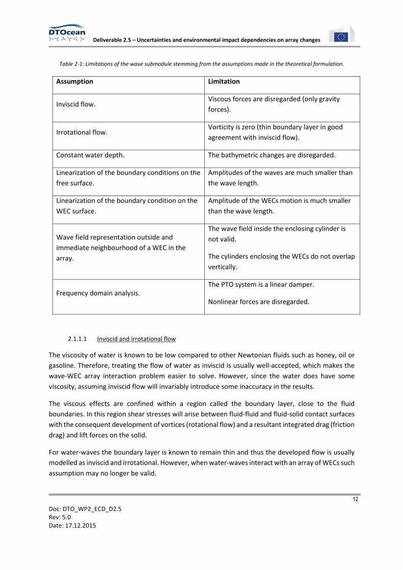
Table 2-1: Limitations of the wave submodule stemming from the assumptions made in the theoretical formulation.
Assumption Limitation
Inviscid flow. Viscous forces are disregarded (only gravity
forces).
Irrotational flow. Vorticity is zero (thin boundary layer in good
agreement with inviscid flow).
Constant water depth. The bathymetric changes are disregarded.
Linearization of the boundary conditions on the
free surface.
Amplitudes of the waves are much smaller than
the wave length.
Linearization of the boundary condition on the
WEC surface.
Amplitude of the WECs motion is much smaller
than the wave length.
Wave field representation outside and
immediate neighbourhood of a WEC in the
array.
The wave field inside the enclosing cylinder is
not valid.
The cylinders enclosing the WECs do not overlap
vertically.
Frequency domain analysis.
The PTO system is a linear damper.
Nonlinear forces are disregarded.
2.1.1.1 Inviscid and irrotational flow
The viscosity of water is known to be low compared to other Newtonian fluids such as honey, oil or
gasoline. Therefore, treating the flow of water as inviscid is usually well-accepted, which makes the
wave-WEC array interaction problem easier to solve. However, since the water does have some
viscosity, assuming inviscid flow will invariably introduce some inaccuracy in the results.
The viscous effects are confined within a region called the boundary layer, close to the fluid
boundaries. In this region shear stresses will arise between fluid-fluid and fluid-solid contact surfaces
with the consequent development of vortices (rotational flow) and a resultant integrated drag (friction
drag) and lift forces on the solid.
For water-waves the boundary layer is known to remain thin and thus the developed flow is usually
modelled as inviscid and irrotational. However, when water-waves interact with an array of WECs such
assumption may no longer be valid.
Deliverable 2.5 – Uncertainties and environmental impact dependencies on array changes
13
Doc: DTO_WP2_ECD_D2.5
Rev: 5.0
Date: 17.12.2015
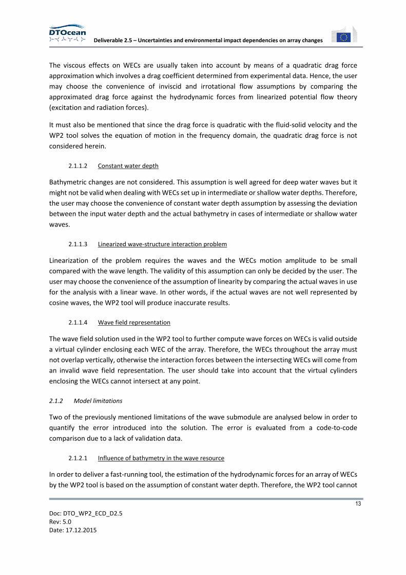
The viscous effects on WECs are usually taken into account by means of a quadratic drag force
approximation which involves a drag coefficient determined from experimental data. Hence, the user
may choose the convenience of inviscid and irrotational flow assumptions by comparing the
approximated drag force against the hydrodynamic forces from linearized potential flow theory
(excitation and radiation forces).
It must also be mentioned that since the drag force is quadratic with the fluid-solid velocity and the
WP2 tool solves the equation of motion in the frequency domain, the quadratic drag force is not
considered herein.
2.1.1.2 Constant water depth
Bathymetric changes are not considered. This assumption is well agreed for deep water waves but it
might not be valid when dealing with WECs set up in intermediate or shallow water depths. Therefore,
the user may choose the convenience of constant water depth assumption by assessing the deviation
between the input water depth and the actual bathymetry in cases of intermediate or shallow water
waves.
2.1.1.3 Linearized wave-structure interaction problem
Linearization of the problem requires the waves and the WECs motion amplitude to be small
compared with the wave length. The validity of this assumption can only be decided by the user. The
user may choose the convenience of the assumption of linearity by comparing the actual waves in use
for the analysis with a linear wave. In other words, if the actual waves are not well represented by
cosine waves, the WP2 tool will produce inaccurate results.
2.1.1.4 Wave field representation
The wave field solution used in the WP2 tool to further compute wave forces on WECs is valid outside
a virtual cylinder enclosing each WEC of the array. Therefore, the WECs throughout the array must
not overlap vertically, otherwise the interaction forces between the intersecting WECs will come from
an invalid wave field representation. The user should take into account that the virtual cylinders
enclosing the WECs cannot intersect at any point.
2.1.2 Model limitations
Two of the previously mentioned limitations of the wave submodule are analysed below in order to
quantify the error introduced into the solution. The error is evaluated from a code-to-code
comparison due to a lack of validation data.
2.1.2.1 Influence of bathymetry in the wave resource
In order to deliver a fast-running tool, the estimation of the hydrodynamic forces for an array of WECs
by the WP2 tool is based on the assumption of constant water depth. Therefore, the WP2 tool cannot
Deliverable 2.5 – Uncertainties and environmental impact dependencies on array changes
14
Doc: DTO_WP2_ECD_D2.5
Rev: 5.0
Date: 17.12.2015
actually reproduce the wave transformations due to changes in water depth. Although this
assumption is suitable for far-offshore arrays, it might not be valid for those arrays sitting close to the
coast. For these arrays, the validity will be invariably related to the magnitude of change in water
depth.
In order to assess the uncertainty of the predicted values by the WP2 tool due to varying water depth,
a comparison of significant wave height (Hm0) values will be carried out between the WP2 tool and
the MIKE 21 software. The MIKE 21 software solves the enhanced Boussinesq equations, which allows
for the modelling of wave phenomena due to water depth variations.
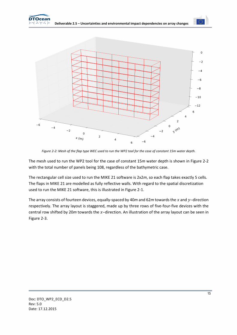
The case study for the comparison to take place is an array of flap type fixed WECs, which span the
water depth and which are hold fixed (i.e. they are not allowed to move). The flaps are modelled as
rectangular boxes of dimension 10x2xhm, with h the water depth.
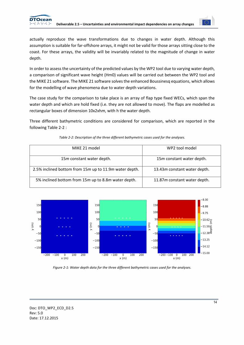
Three different bathymetric conditions are considered for comparison, which are reported in the
following Table 2-2 :
Table 2-2: Description of the three different bathymetric cases used for the analyses.
MIKE 21 model WP2 tool model
15m constant water depth. 15m constant water depth.
2.5% inclined bottom from 15m up to 11.9m water depth. 13.43m constant water depth.
5% inclined bottom from 15m up to 8.8m water depth. 11.87m constant water depth.
Figure 2-1: Water depth data for the three different bathymetric cases used for the analyses.
Deliverable 2.5 – Uncertainties and environmental impact dependencies on array changes
15
Doc: DTO_WP2_ECD_D2.5
Rev: 5.0
Date: 17.12.2015
Figure 2-2: Mesh of the flap type WEC used to run the WP2 tool for the case of constant 15m water depth.
The mesh used to run the WP2 tool for the case of constant 15m water depth is shown in Figure 2-2
with the total number of panels being 108, regardless of the bathymetric case.
The rectangular cell size used to run the MIKE 21 software is 2x2m, so each flap takes exactly 5 cells.
The flaps in MIKE 21 are modelled as fully reflective walls. With regard to the spatial discretization
used to run the MIKE 21 software, this is illustrated in Figure 2-1.
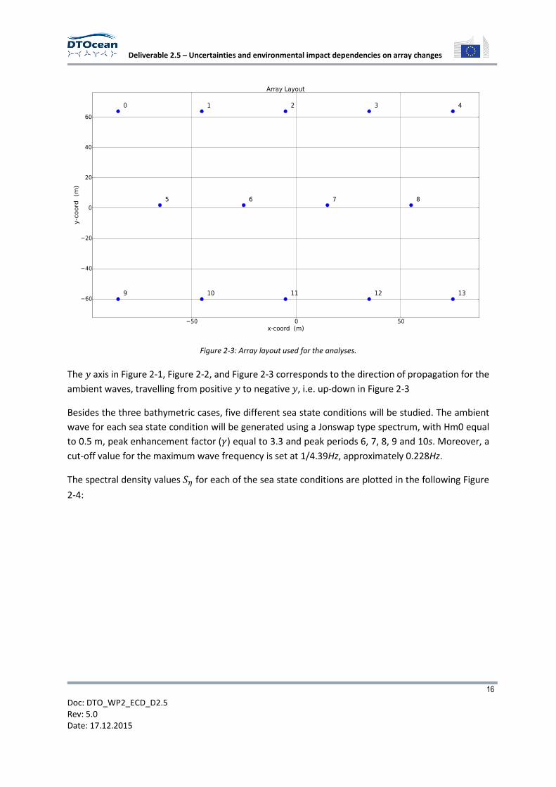
The array consists of fourteen devices, equally-spaced by 40m and 62m towards the � and �‒direction
respectively. The array layout is staggered, made up by three rows of five-four-five devices with the
central row shifted by 20m towards the �‒direction. An illustration of the array layout can be seen in
Figure 2-3.
Deliverable 2.5 – Uncertainties and environmental impact dependencies on array changes
16
Doc: DTO_WP2_ECD_D2.5
Rev: 5.0
Date: 17.12.2015
Figure 2-3: Array layout used for the analyses.
The � axis in Figure 2-1, Figure 2-2, and Figure 2-3 corresponds to the direction of propagation for the
ambient waves, travelling from positive � to negative �, i.e. up-down in Figure 2-3
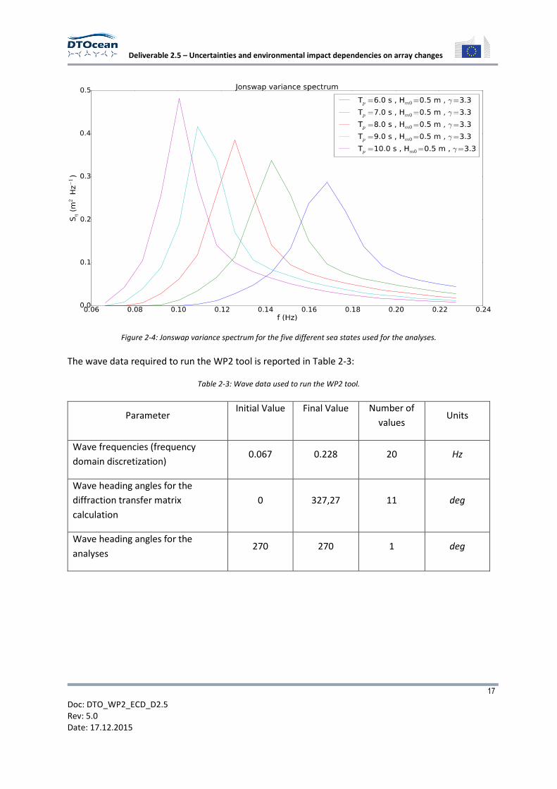
Besides the three bathymetric cases, five different sea state conditions will be studied. The ambient
wave for each sea state condition will be generated using a Jonswap type spectrum, with Hm0 equal
to 0.5 m, peak enhancement factor (�) equal to 3.3 and peak periods 6, 7, 8, 9 and 10s. Moreover, a
cut-off value for the maximum wave frequency is set at 1/4.39Hz, approximately 0.228Hz.
The spectral density values �� for each of the sea state conditions are plotted in the following Figure
2-4:
Deliverable 2.5 – Uncertainties and environmental impact dependencies on array changes
17
Doc: DTO_WP2_ECD_D2.5
Rev: 5.0
Date: 17.12.2015
Figure 2-4: Jonswap variance spectrum for the five different sea states used for the analyses.
The wave data required to run the WP2 tool is reported in Table 2-3:
Table 2-3: Wave data used to run the WP2 tool.
Parameter Initial Value Final Value Number of
values Units
Wave frequencies (frequency
domain discretization) 0.067 0.228 20 Hz
Wave heading angles for the
diffraction transfer matrix
calculation
0 327,27 11 deg
Wave heading angles for the
analyses 270 270 1 deg
Deliverable 2.5 – Uncertainties and environmental impact dependencies on array changes
18
Doc: DTO_WP2_ECD_D2.5
Rev: 5.0
Date: 17.12.2015
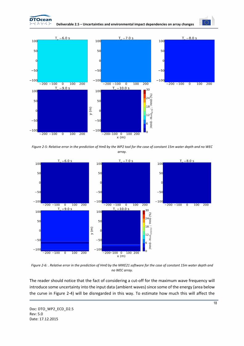
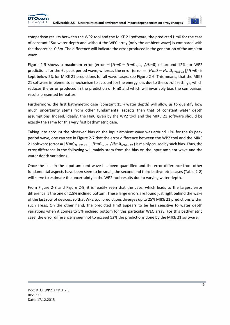
Figure 2-5: Relative error in the prediction of Hm0 by the WP2 tool for the case of constant 15m water depth and no WEC
array.
Figure 2-6: . Relative error in the prediction of Hm0 by the MIKE21 software for the case of constant 15m water depth and
no WEC array.
The reader should notice that the fact of considering a cut-off for the maximum wave frequency will
introduce some uncertainty into the input data (ambient waves) since some of the energy (area below
the curve in Figure 2-4) will be disregarded in this way. To estimate how much this will affect the
Deliverable 2.5 – Uncertainties and environmental impact dependencies on array changes
19
Doc: DTO_WP2_ECD_D2.5
Rev: 5.0
Date: 17.12.2015
comparison results between the WP2 tool and the MIKE 21 software, the predicted Hm0 for the case
of constant 15m water depth and without the WEC array (only the ambient wave) is compared with
the theoretical 0.5m. The difference will indicate the error produced in the generation of the ambient
wave.
Figure 2-5 shows a maximum error (error � |0 � 0 ��| 0⁄ ) of around 12% for WP2
predictions for the 6s peak period wave, whereas the error (error � |0 � 0������| 0⁄ ) is
kept below 5% for MIKE 21 predictions for all wave cases, see Figure 2-6. This means, that the MIKE
21 software implements a mechanism to account for the energy loss due to the cut-off settings, which
reduces the error produced in the prediction of Hm0 and which will invariably bias the comparison
results presented hereafter.
Furthermore, the first bathymetric case (constant 15m water depth) will allow us to quantify how
much uncertainty stems from other fundamental aspects than that of constant water depth
assumptions. Indeed, ideally, the Hm0 given by the WP2 tool and the MIKE 21 software should be
exactly the same for this very first bathymetric case.
Taking into account the observed bias on the input ambient wave was around 12% for the 6s peak
period wave, one can see in Figure 2-7 that the error difference between the WP2 tool and the MIKE
21 software (error � |0������ � 0 ��| 0������⁄ ) is mainly caused by such bias. Thus, the
error difference in the following will mainly stem from the bias on the input ambient wave and the
water depth variations.
Once the bias in the input ambient wave has been quantified and the error difference from other
fundamental aspects have been seen to be small, the second and third bathymetric cases (Table 2-2)
will serve to estimate the uncertainty in the WP2 tool results due to varying water depth.
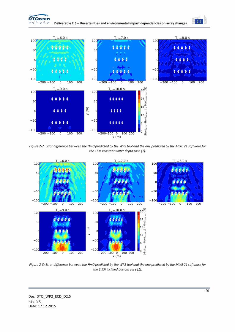
From Figure 2-8 and Figure 2-9, it is readily seen that the case, which leads to the largest error
difference is the one of 2.5% inclined bottom. These large errors are found just right behind the wake
of the last row of devices, so that WP2 tool predictions diverges up to 25% MIKE 21 predictions within
such areas. On the other hand, the predicted Hm0 appears to be less sensitive to water depth
variations when it comes to 5% inclined bottom for this particular WEC array. For this bathymetric
case, the error difference is seen not to exceed 12% the predictions done by the MIKE 21 software.
Deliverable 2.5 – Uncertainties and environmental impact dependencies on array changes
20
Doc: DTO_WP2_ECD_D2.5
Rev: 5.0
Date: 17.12.2015
Figure 2-7: Error difference between the Hm0 predicted by the WP2 tool and the one predicted by the MIKE 21 software for
the 15m constant water depth case [1].
Figure 2-8: Error difference between the Hm0 predicted by the WP2 tool and the one predicted by the MIKE 21 software for
the 2.5% inclined bottom case [1].

Deliverable 2.5 – Uncertainties and environmental impact dependencies on array changes
21
Doc: DTO_WP2_ECD_D2.5
Rev: 5.0
Date: 17.12.2015
Figure 2-9: Error difference between the Hm0 predicted by the WP2 tool and the one predicted by the MIKE 21 software for
the 5% inclined bottom case [1].
Overall, it is seen that wave transformations effects due to water depth variations can lead up to 25%
uncertainty to Hm0 predictions. Since the Hm0 is a measure of the total wave energy content, it seems
apparent that water depth variation effects play an important role when predicting the total power
output of WEC arrays placed near the shore.
2.1.2.2 Influence of wave directional spreading into the hydrodynamci interaction
Another important limitation of the interaction theory based on BEM solutions is that the body is not
assumed to move from the initial equilibrium position.
This assumption forces the relative position between bodies to be fixed, and therefore, within an
array, highly destructive or constructive interaction can build up, even if not entirely realistic.
In a real scenario the bodies will move around the equilibrium position and most likely
constrictive/destructive interaction will be averaged in time.
Since the model is built in the frequency domain it is not possible to include this type of non-linearity
in the solution, and a simple approach to estimate this energy dissipation is to distribute the energy
content around the main direction using a spreading function.
In this way, for each wave direction, the relative distance between bodies will vary, creating a
smoothing effect on the constructive/destructive hydrodynamic interaction.
Deliverable 2.5 – Uncertainties and environmental impact dependencies on array changes
22
Doc: DTO_WP2_ECD_D2.5
Rev: 5.0
Date: 17.12.2015
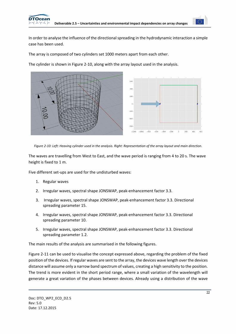
In order to analyse the influence of the directional spreading in the hydrodynamic interaction a simple
case has been used.
The array is composed of two cylinders set 1000 meters apart from each other.
The cylinder is shown in Figure 2-10, along with the array layout used in the analysis.
Figure 2-10: Left: Heaving cylinder used in the analysis. Right: Representation of the array layout and main direction.
The waves are travelling from West to East, and the wave period is ranging from 4 to 20 s. The wave
height is fixed to 1 m.
Five different set-ups are used for the undisturbed waves:
1. Regular waves
2. Irregular waves, spectral shape JONSWAP, peak-enhancement factor 3.3.
3. Irregular waves, spectral shape JONSWAP, peak-enhancement factor 3.3. Directional
spreading parameter 15.
4. Irregular waves, spectral shape JONSWAP, peak-enhancement factor 3.3. Directional
spreading parameter 10.
5. Irregular waves, spectral shape JONSWAP, peak-enhancement factor 3.3. Directional
spreading parameter 1.2.
The main results of the analysis are summarised in the following figures.
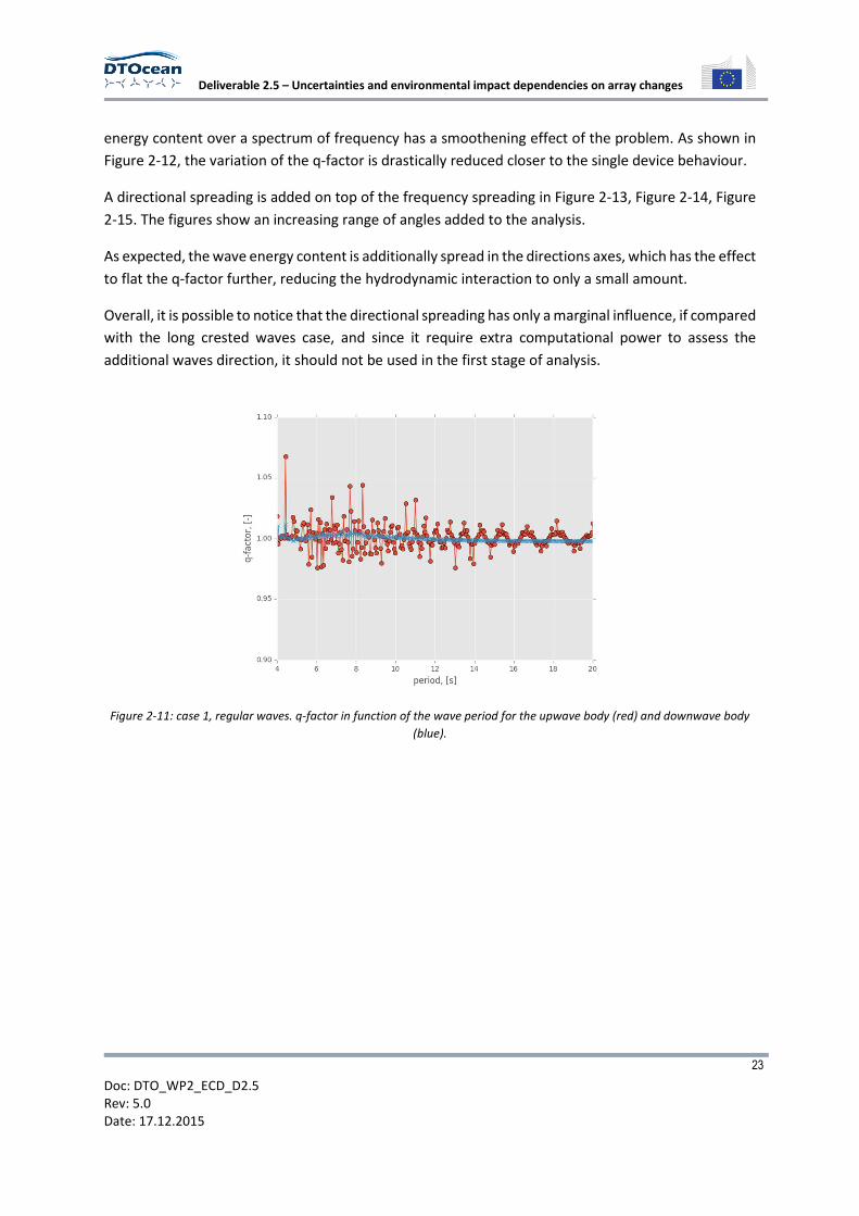
Figure 2-11 can be used to visualise the concept expressed above, regarding the problem of the fixed
position of the devices. If regular waves are sent to the array, the devices wave length over the devices
distance will assume only a narrow band spectrum of values, creating a high sensitivity to the position.
The trend is more evident in the short period range, where a small variation of the wavelength will
generate a great variation of the phases between devices. Already using a distribution of the wave
Deliverable 2.5 – Uncertainties and environmental impact dependencies on array changes
23
Doc: DTO_WP2_ECD_D2.5
Rev: 5.0
Date: 17.12.2015
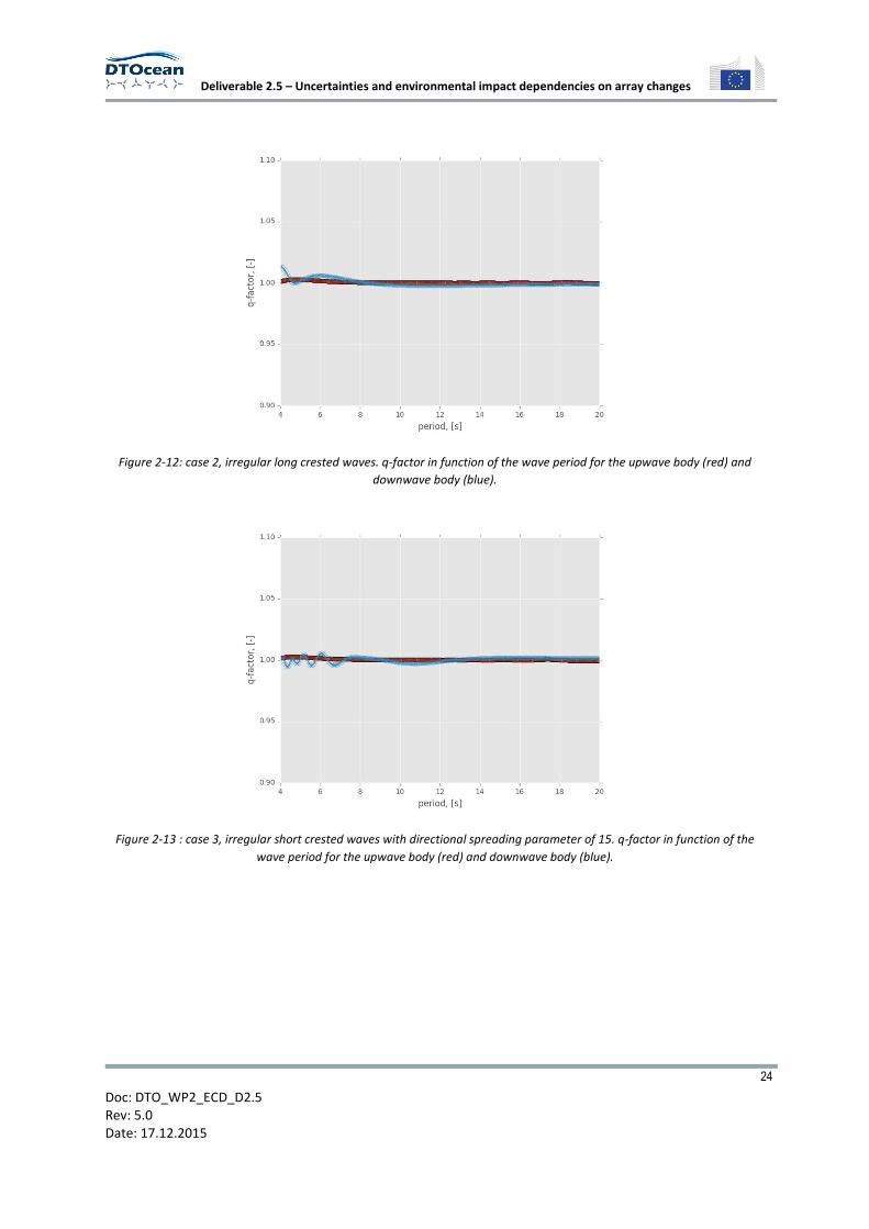
energy content over a spectrum of frequency has a smoothening effect of the problem. As shown in
Figure 2-12, the variation of the q-factor is drastically reduced closer to the single device behaviour.
A directional spreading is added on top of the frequency spreading in Figure 2-13, Figure 2-14, Figure
2-15. The figures show an increasing range of angles added to the analysis.
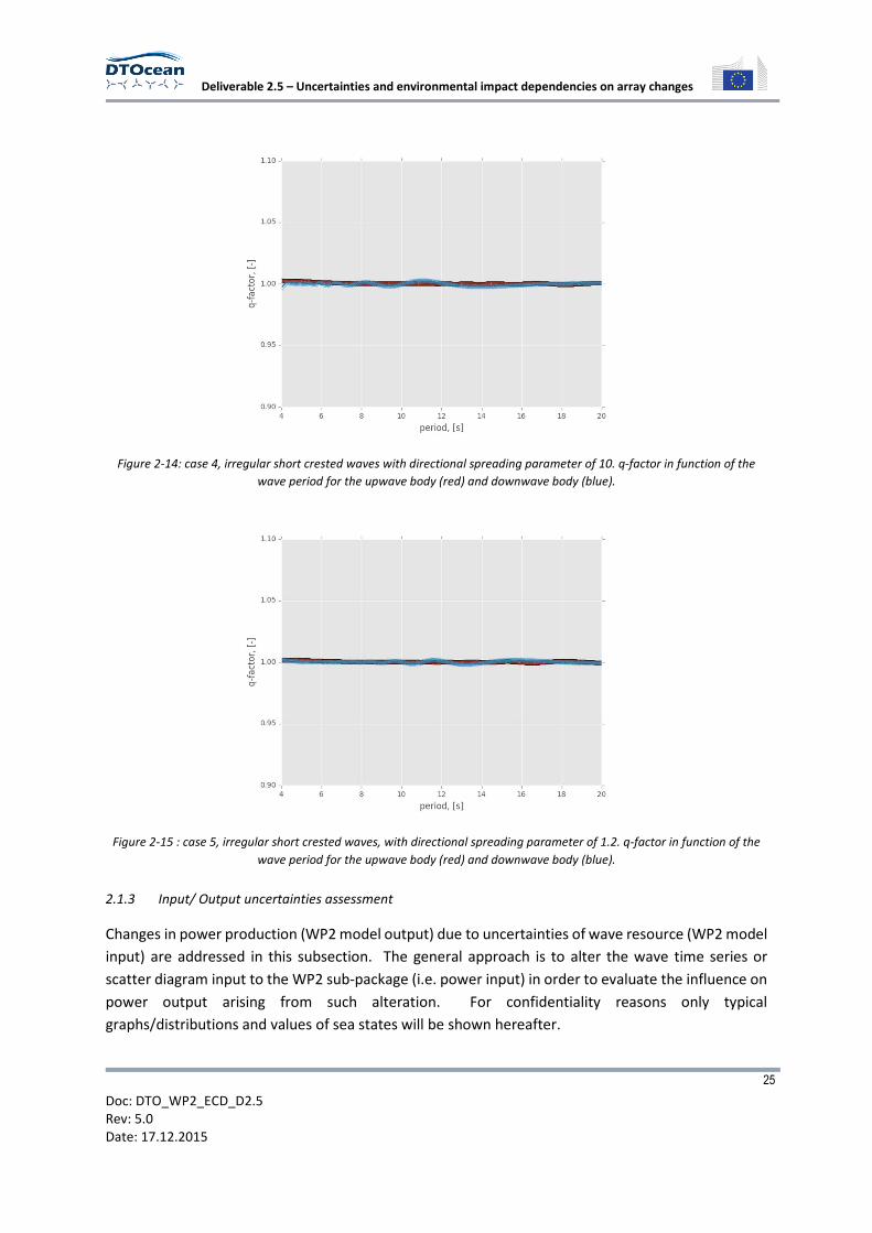
As expected, the wave energy content is additionally spread in the directions axes, which has the effect
to flat the q-factor further, reducing the hydrodynamic interaction to only a small amount.
Overall, it is possible to notice that the directional spreading has only a marginal influence, if compared
with the long crested waves case, and since it require extra computational power to assess the
additional waves direction, it should not be used in the first stage of analysis.
Figure 2-11: case 1, regular waves. q-factor in function of the wave period for the upwave body (red) and downwave body
(blue).
Deliverable 2.5 – Uncertainties and environmental impact dependencies on array changes
24
Doc: DTO_WP2_ECD_D2.5
Rev: 5.0
Date: 17.12.2015
Figure 2-12: case 2, irregular long crested waves. q-factor in function of the wave period for the upwave body (red) and
downwave body (blue).
Figure 2-13 : case 3, irregular short crested waves with directional spreading parameter of 15. q-factor in function of the
wave period for the upwave body (red) and downwave body (blue).
Deliverable 2.5 – Uncertainties and environmental impact dependencies on array changes
25
Doc: DTO_WP2_ECD_D2.5
Rev: 5.0
Date: 17.12.2015
Figure 2-14: case 4, irregular short crested waves with directional spreading parameter of 10. q-factor in function of the
wave period for the upwave body (red) and downwave body (blue).
Figure 2-15 : case 5, irregular short crested waves, with directional spreading parameter of 1.2. q-factor in function of the
wave period for the upwave body (red) and downwave body (blue).
2.1.3 Input/ Output uncertainties assessment
Changes in power production (WP2 model output) due to uncertainties of wave resource (WP2 model
input) are addressed in this subsection. The general approach is to alter the wave time series or
scatter diagram input to the WP2 sub-package (i.e. power input) in order to evaluate the influence on
power output arising from such alteration. For confidentiality reasons only typical
graphs/distributions and values of sea states will be shown hereafter.
Deliverable 2.5 – Uncertainties and environmental impact dependencies on array changes
26
Doc: DTO_WP2_ECD_D2.5
Rev: 5.0
Date: 17.12.2015
Two different investigations are carried out:
• Statistical approach - Investigate uncertainties of the input scatter diagram
• Deterministic approach - Sensitivity analysis of the power input
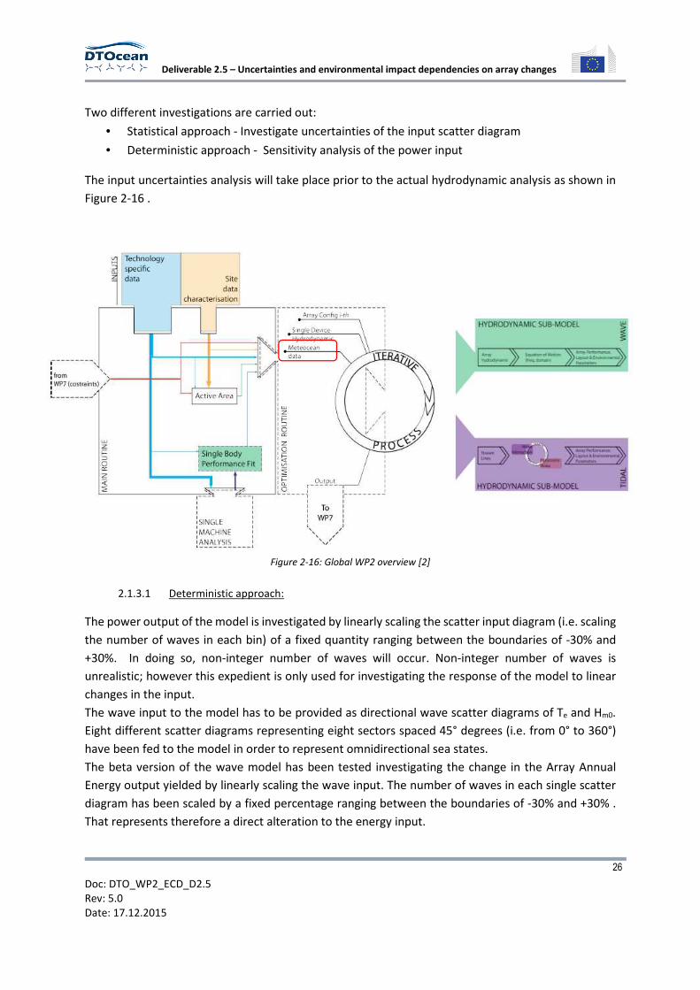
The input uncertainties analysis will take place prior to the actual hydrodynamic analysis as shown in
Figure 2-16 .
Figure 2-16: Global WP2 overview [2]
2.1.3.1 Deterministic approach:
The power output of the model is investigated by linearly scaling the scatter input diagram (i.e. scaling
the number of waves in each bin) of a fixed quantity ranging between the boundaries of -30% and
+30%. In doing so, non-integer number of waves will occur. Non-integer number of waves is
unrealistic; however this expedient is only used for investigating the response of the model to linear
changes in the input.
The wave input to the model has to be provided as directional wave scatter diagrams of Te and Hm0.
Eight different scatter diagrams representing eight sectors spaced 45° degrees (i.e. from 0° to 360°)
have been fed to the model in order to represent omnidirectional sea states.
The beta version of the wave model has been tested investigating the change in the Array Annual
Energy output yielded by linearly scaling the wave input. The number of waves in each single scatter
diagram has been scaled by a fixed percentage ranging between the boundaries of -30% and +30% .
That represents therefore a direct alteration to the energy input.

Deliverable 2.5 – Uncertainties and environmental impact dependencies on array changes
27
Doc: DTO_WP2_ECD_D2.5
Rev: 5.0
Date: 17.12.2015
An example of linear scaling of scatter diagrams for the directional sector 270°-315° (i.e. the sector
with highest energy content) is shown in Figure 2-17.
-
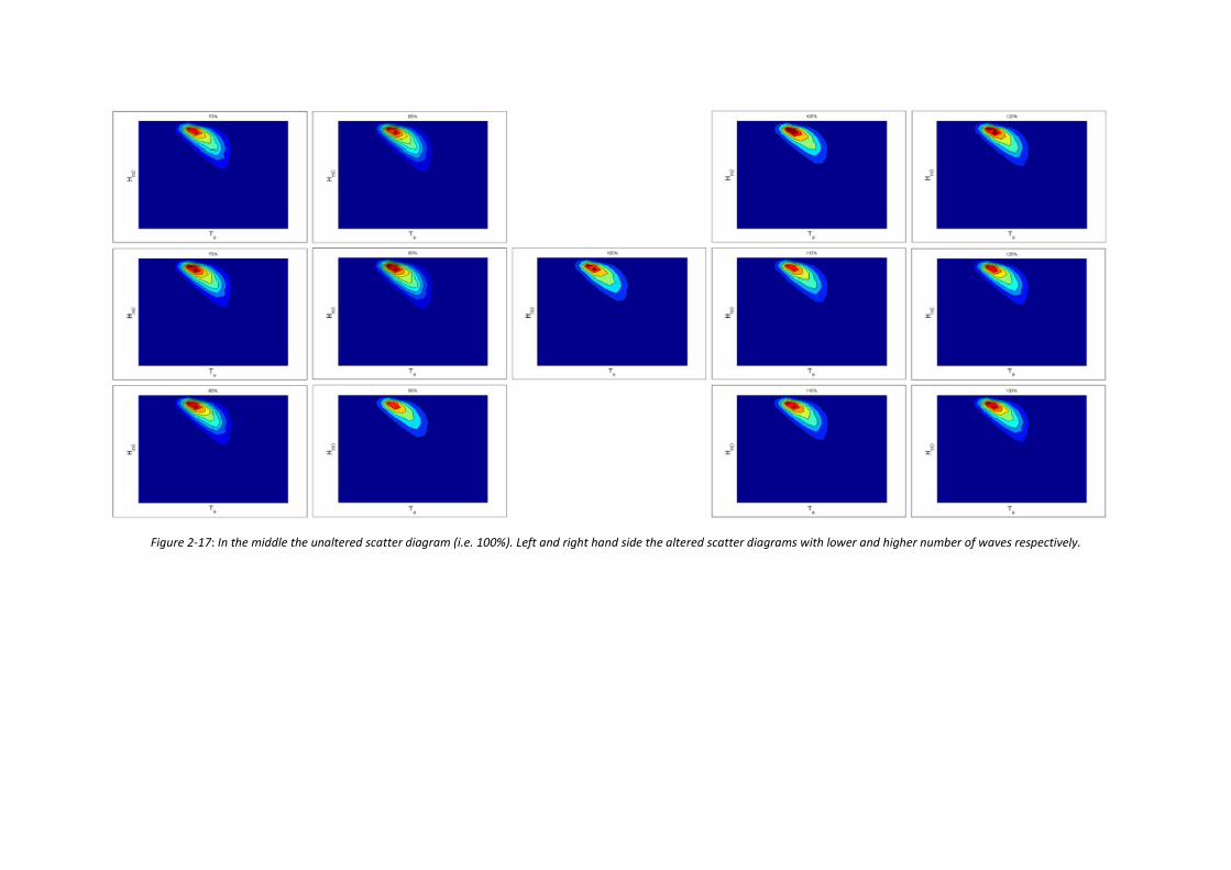
Figure 2-17: In the middle the unaltered scatter diagram (i.e. 100%). Left and right hand side the altered scatter diagrams with lower and higher number of waves respectively.
Deliverable 2.5 – Uncertainties and environmental impact dependencies on array changes
29
Doc: DTO_WP2_ECD_D2.5
Rev: 4.2
Date: 01.12.2015
It is important to remark that since the model is at its beta version at the date of this, not all
functionalities of the wave model have been activated.
Due to the approach used to solve the hydrodynamics (i.e. linear theory), it is expected that a linear
change in the power input (i.e. number of waves) should be linearly reflected in the power output.
Simple conditions for simulation have been set up in order to have an easy check on the outputs at
the beta version stage.
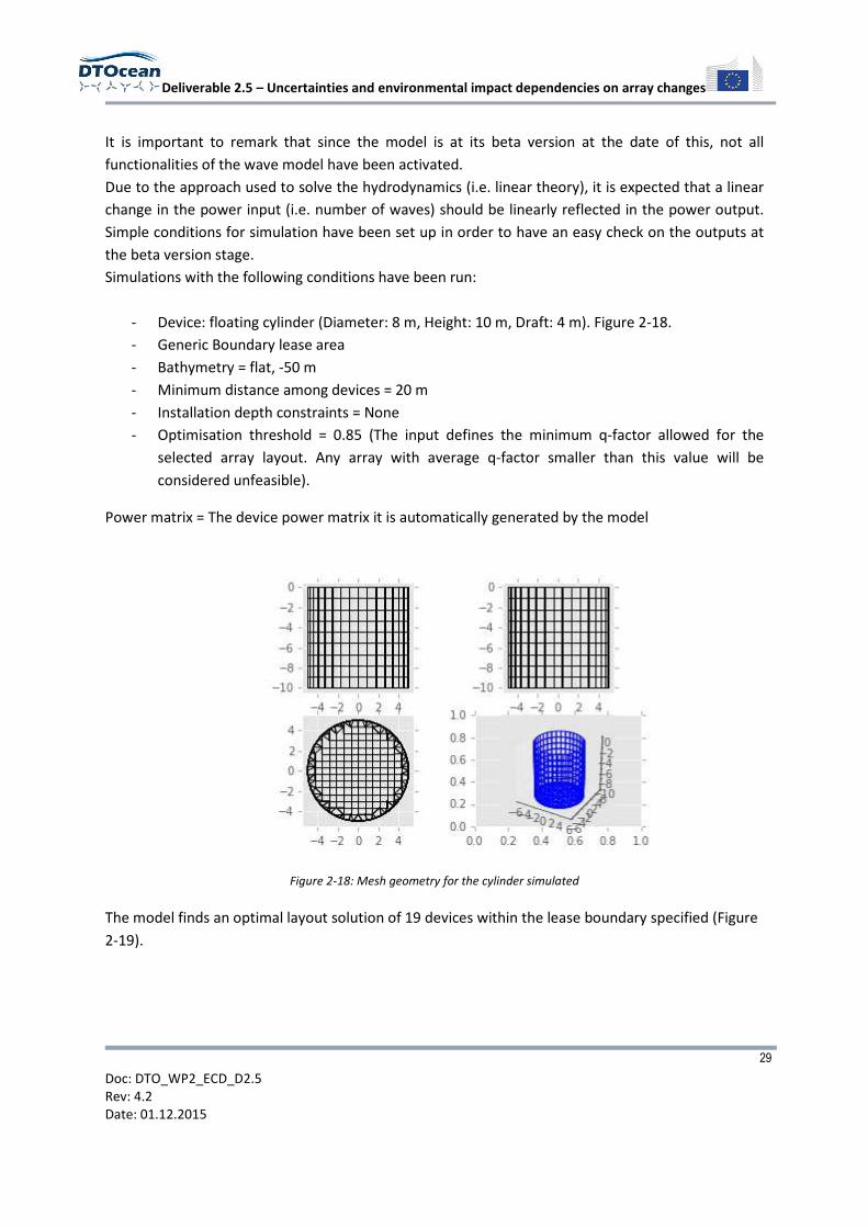
Simulations with the following conditions have been run:
- Device: floating cylinder (Diameter: 8 m, Height: 10 m, Draft: 4 m). Figure 2-18.
- Generic Boundary lease area
- Bathymetry = flat, -50 m
- Minimum distance among devices = 20 m
- Installation depth constraints = None
- Optimisation threshold = 0.85 (The input defines the minimum q-factor allowed for the
selected array layout. Any array with average q-factor smaller than this value will be
considered unfeasible).
Power matrix = The device power matrix it is automatically generated by the model
Figure 2-18: Mesh geometry for the cylinder simulated
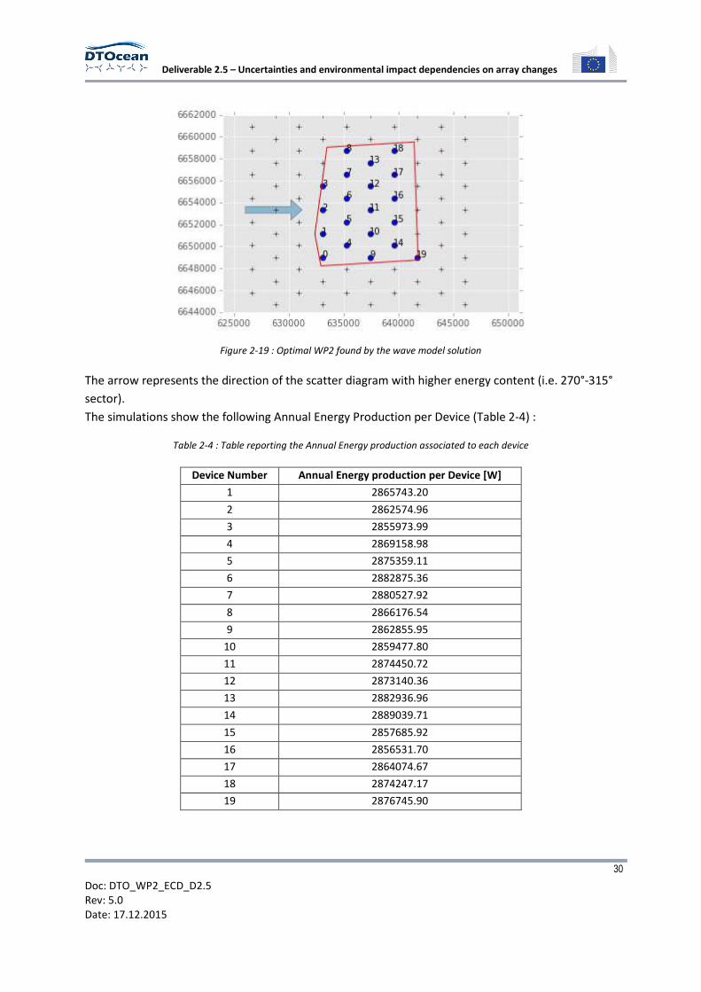
The model finds an optimal layout solution of 19 devices within the lease boundary specified (Figure
2-19).
Deliverable 2.5 – Uncertainties and environmental impact dependencies on array changes
30
Doc: DTO_WP2_ECD_D2.5
Rev: 5.0
Date: 17.12.2015
Figure 2-19 : Optimal WP2 found by the wave model solution
The arrow represents the direction of the scatter diagram with higher energy content (i.e. 270°-315°
sector).
The simulations show the following Annual Energy Production per Device (Table 2-4) :
Table 2-4 : Table reporting the Annual Energy production associated to each device
Device Number Annual Energy production per Device [W]
1 2865743.20
2 2862574.96
3 2855973.99
4 2869158.98
5 2875359.11
6 2882875.36
7 2880527.92
8 2866176.54
9 2862855.95
10 2859477.80
11 2874450.72
12 2873140.36
13 2882936.96
14 2889039.71
15 2857685.92
16 2856531.70
17 2864074.67
18 2874247.17
19 2876745.90
Deliverable 2.5 – Uncertainties and environmental impact dependencies on array changes
31
Doc: DTO_WP2_ECD_D2.5
Rev: 5.0
Date: 17.12.2015
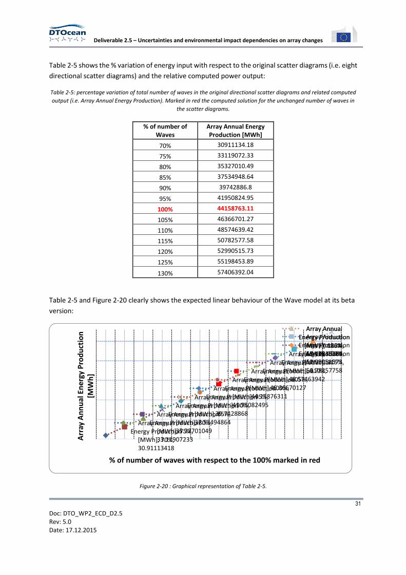
Table 2-5 shows the % variation of energy input with respect to the original scatter diagrams (i.e. eight
directional scatter diagrams) and the relative computed power output:
Table 2-5: percentage variation of total number of waves in the original directional scatter diagrams and related computed
output (i.e. Array Annual Energy Production). Marked in red the computed solution for the unchanged number of waves in
the scatter diagrams.
% of number of
Waves
Array Annual Energy
Production [MWh]
70% 30911134.18
75% 33119072.33
80% 35327010.49
85% 37534948.64
90% 39742886.8
95% 41950824.95
100% 44158763.11
105% 46366701.27
110% 48574639.42
115% 50782577.58
120% 52990515.73
125% 55198453.89
130% 57406392.04
Table 2-5 and Figure 2-20 clearly shows the expected linear behaviour of the Wave model at its beta
version:
Figure 2-20 : Graphical representation of Table 2-5.
Array Annual
Energy Production
[MWh], 70%,
30.91113418
Array Annual
Energy Production
[MWh], 75%,
33.11907233
Array Annual
Energy Production
[MWh], 80%,
35.32701049
Array Annual
Energy Production
[MWh], 85%,
37.53494864
Array Annual
Energy Production
[MWh], 90%,
39.7428868
Array Annual
Energy Production
[MWh], 95%,
41.95082495
Array Annual
Energy Production
[MWh], 100%,
44.15876311
Array Annual
Energy Production
[MWh], 105%,
46.36670127
Array Annual
Energy Production
[MWh], 110%,
48.57463942
Array Annual
Energy Production
[MWh], 115%,
50.78257758
Array Annual
Energy Production
[MWh], 120%,
52.99051573
Array Annual
Energy Production
[MWh], 125%,
55.19845389
Array Annual
Energy Production
[MWh], 130%,
57.40639204
Arr
ay
An
nu
al
En
erg
y P
rod
uct
ion
[MW
h]
% of number of waves with respect to the 100% marked in red
Deliverable 2.5 – Uncertainties and environmental impact dependencies on array changes
32
Doc: DTO_WP2_ECD_D2.5
Rev: 5.0
Date: 17.12.2015
2.1.3.2 Statistical Approach:
This section addresses the influence of resource variability on the power outuput by means of a
simplfied statistical apporach.
The WP2 wave hydrodynamic package takes a scatter diagram (i.e. Hm0 , Te) as input, produced by
appropriate binning of the time series of spectral wave height Hm0 and energy period Te.
However, the time series represents only a limited sample of the population of Hm0 and Te. The size of
the time series sample is denoted by N.
Some approaches exist to compute the joint distribution of environmental variables (e.g. Maximum
Likelyhood Model, Conditional Modelling Approach) [3]. However, little is known about the joint
distribution of Hm0 and Te .
Although energy period can be derived from the peak period if the sea spectrum is known [4], this
adds an additional level of complexity and uncertainty when it comes to estimating the joint
probability distribution of Hm0 and Te.
A simplified approach for the assesment of uncertainties in the sea state input is used in Task 2.6.
The key assumption is that the the variables Hm0 and Te are independent and therefore their joint
probabilty distribution can be calculated as follows :
����,������, ��� � ��������� ∙ �������
As opposed to :
!"#$,%&�'(, )*� � !%&|"#$
�)*|'(� ∙ !"+�'(� � !"#$|%&�'(|)*� ∙ !%&�)*�
Therefore, the joint probaility density function (PDF) of Hm0 and Te can be calculated as the product of
the respective marginal PDF. This will allow the recomputation of a scatter diagram without knowing
the conditional distributions !%&|"#$�)*|'(�or !"#$|%&
�'(|)*�.
A wave time series can be binned into equally spaced classes of Hm0 and Te, and the marginal frequency
of occurrence of these variables can be drawn.
The number of bins Nb and their boundaries will be kept unchanged throughout the statistical
approach. In the example that will be shown thereafter a bin spacing of 0.5m and 1s is used
respectively for Hm0 and Te as advised by the IEC Standards [5]. The significant wave height bins range
from 0m to 14m whereas the energy period goes from 0s to a maximum of 22s in order to capture all
the seastates from the origainal data.

Deliverable 2.5 – Uncertainties and environmental impact dependencies on array changes
33
Doc: DTO_WP2_ECD_D2.5
Rev: 5.0
Date: 17.12.2015
For demonstration purposes a 14 year timeseries (1980 - 2013) at hourly resolution of Hm0 and relative
Tp has been used. The peak period (Tp) has been converted to energy period by standard integration
of the wave spectrum [4]. A parametrised Pierson-Moskowitz spectrum has been assumed [6]. Wave
time series is relative to Scenario 1 – North West Lewis [7] at a nearshore point (exact coordinates
cannot be shown for confidentiality reasons).
A typical wave rose for the North West Lewis location can be found in Deliverable 2.2 [8] from which
it can be seen that the predominant wave direction is East/North-East. Therefore, a statistical
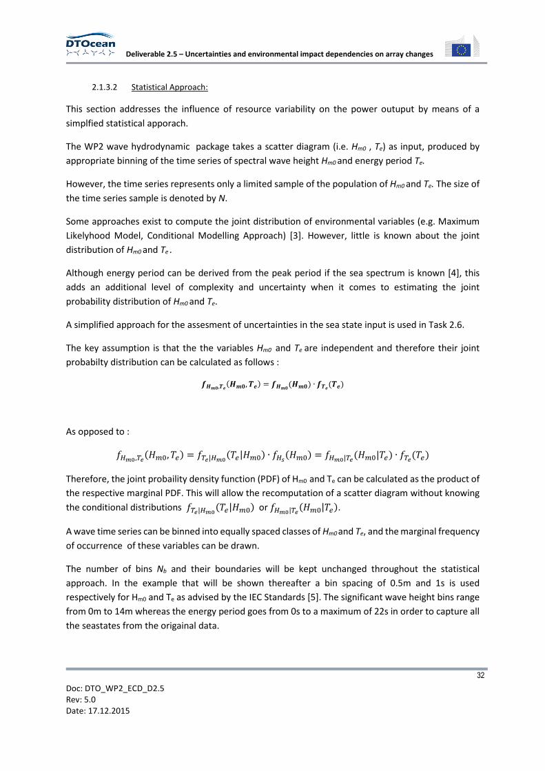
approach for simplicity will only be applied to the directional sector 270°-315° N. Figure 2-21 shows
the scatter diagram associated to this directional sector. For confidentiality reasons the actual data
cannot be shown.
Deliverable 2.5 – Uncertainties and environmental impact dependencies on array changes
34
Doc: DTO_WP2_ECD_D2.5
Rev: 5.0
Date: 17.12.2015
Figure 2-21: 270°-315° N Directional Scatter Diagram with related bar charts of Hm0 and Te. Each bin represents the number of waves. Actual data cannot be shown for confidentiality reasons.

Deliverable 2.5 – Uncertainties and environmental impact dependencies on array changes
35
Doc: DTO_WP2_ECD_D2.5
Rev: 5.0
Date: 17.12.2015
A second assumption of this methodology is to assume that it is possible to fit the time series sample
with a probability distribution for the variable Hm0. That is in theory always possible although the
quality of the fit has to be verified as it may not be possible to adequately discriminate the tail
behaviour. This method is also known as “the global model”[3] or “total sample method [9].
Opposite to Hm0 , the Te time series will not be fitted to any probability distribution and only its
marginal frequency of occurrence will be used.
The Hm0 sample time series is fitted to a probability distribution curve using standard methods (e.g.
Graphical Fitting, Methods of Moments, Least Squares Methods, Maximum Likelyhood Estimations
[3]. It is assumed that the sample probability distribution represents the “true” population probability
distribution of the variable Hm0 .
Hereafter is shown an example of the statistical approach to produce a scatter diagram that takes into
account the statistical variability of the seastate. The scatter diagram thus generated will be fed to the
WP2 subpackages and the output will be compared with the output resulting from applying the
original (i.e. non-altered) scatter diagram.
For simplicity only a directional scatter diagram relative to the predomimnat wave direction is utilised.
That wave sector is identified as 270°-315° N. The total number of waves considered is N.
Unless data indicates otherwise, a 3-parameter Weibull distribution can be assumed for the marginal
distribution of significant wave height Hm0 [3]. The example below shows a typical Weibull distribution:
−−
−=
β
αγ0
01( )0
m
m
H
mH eHP
where α is the scale parameter, β is the shape parameter, and γ is the location parameter.The
distribution parameters are determined from site specific data by a fitting technique [3].
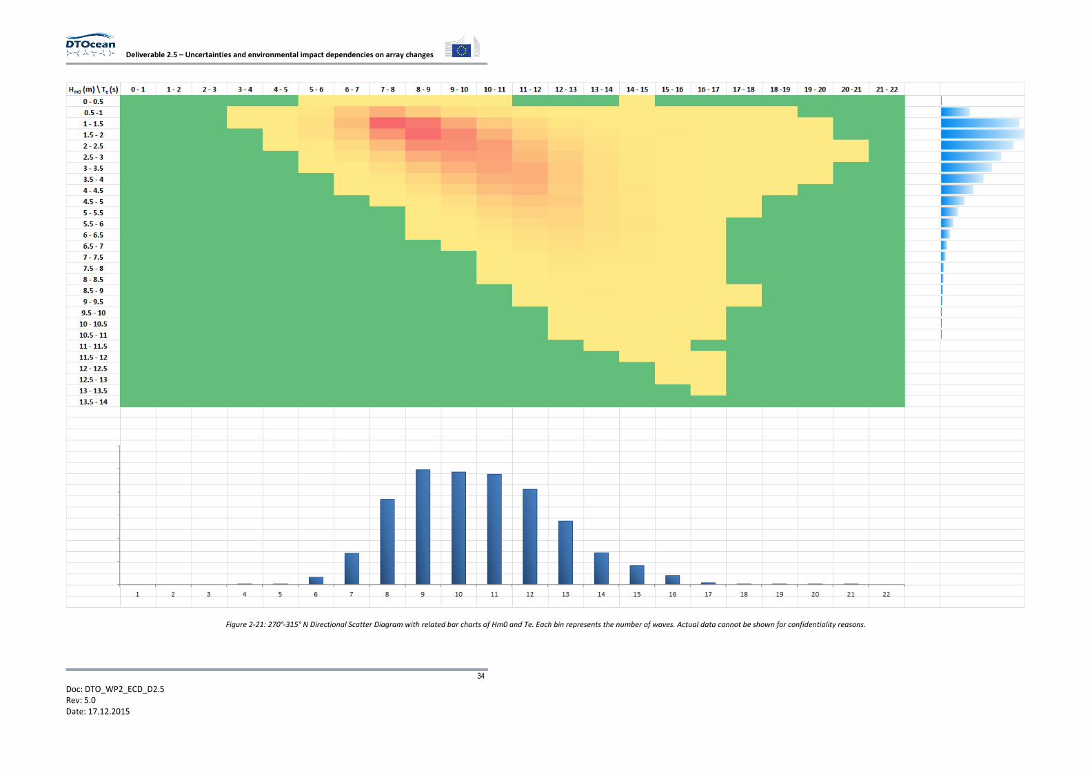
Figure 2-22 shows a typical marginal frequency of occurrence as a % of the significant wave height
(i.e. Hm0) time series. This marginal frequency of occurrence will be used to show how the new scatter
diagram can be derived :
Deliverable 2.5 – Uncertainties and environmental impact dependencies on array changes
36
Doc: DTO_WP2_ECD_D2.5
Rev: 5.0
Date: 17.12.2015
Figure 2-22: Typical Hm0 marginal frequency of occurrence (as a percentage)
The best fit returns the parameters that describe the CDF (or alternatevely the PDF). These parameters
will be representative of the true CDF distribution. Figure 2-23 shows the Weibull CDF applied to the
West Lewis time series:
Figure 2-23: Example of the fitting of a theoretical Weibull CDF to the sample cumulative frequency of occurrence.
Once the probability distribution is assumed known, a Monte Carlo simulation is performed in order
to reproduce random samples of the Hm0 population. The size of samples is N as in the original time
series.
Deliverable 2.5 – Uncertainties and environmental impact dependencies on array changes
37
Doc: DTO_WP2_ECD_D2.5
Rev: 5.0
Date: 17.12.2015
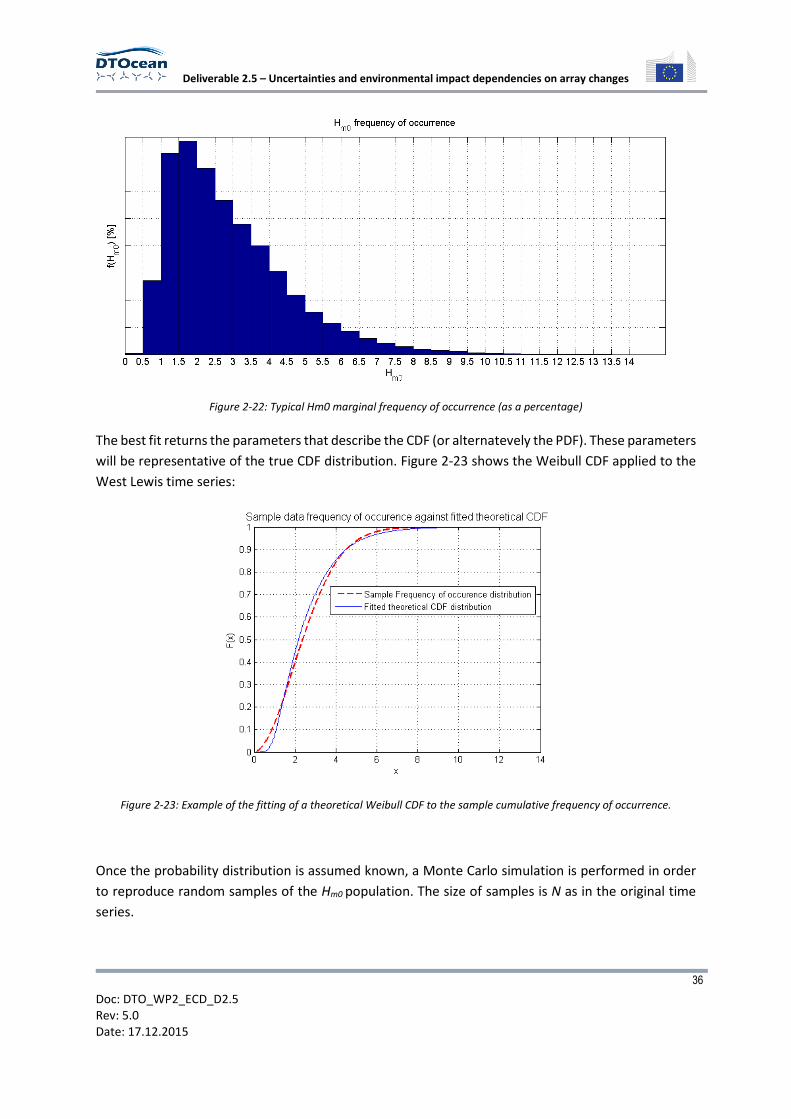
The Monte Carlo simualtion is run M times. Each time, the m-th sample of size N is binned using the
same bin boundaries (i.e. the same numbers of bins Nb) as the original scatter diagram bin boundaries
for the variable Hm0 .
The final outcome of the simulation is a matrix M x Nb of frequency of occurrence for each bin.
If M is big enough, say at least M =10000, the distribution of the frequency of occurrence of each bin
follows a normal distribution.
Figure 2-24 shows the normal distribution shape of the frequency of occurrence for Bin number = 10
corresponding to the interval 4.5 m ≤ Hm0 < 5.0 m .
Figure 2-24: Frequency distribution of the frequency of occurrence for bin No. 10 (i.e 4.5 m ≤ Hm0 < 5.0 m) after Monte
Carlo simulation
Since the “true” standard deviation of the normal distribution for the frequency of occurrence of each
bin is unknown, the Student’s-t distribution with n-1 degree of freedom is applied [10]. A level of
significance α can be fixed, and therefore confidence interval (CI) values can be defined for each bin
frequency of occurrence. The relationship between the the level of significance α and the confidence
interval is as follows :
CI=1- α
Where α ranges between 0 and 1.
Confidence intervals for the mean value of the Student’s-t distribution of the frequency of occurrence
for each bin can therefore be calculated for different levels of significance α.
When treating metocean data a widely used CI value is 95% (i.e. corresponding to α=5%).
Deliverable 2.5 – Uncertainties and environmental impact dependencies on array changes
38
Doc: DTO_WP2_ECD_D2.5
Rev: 5.0
Date: 17.12.2015
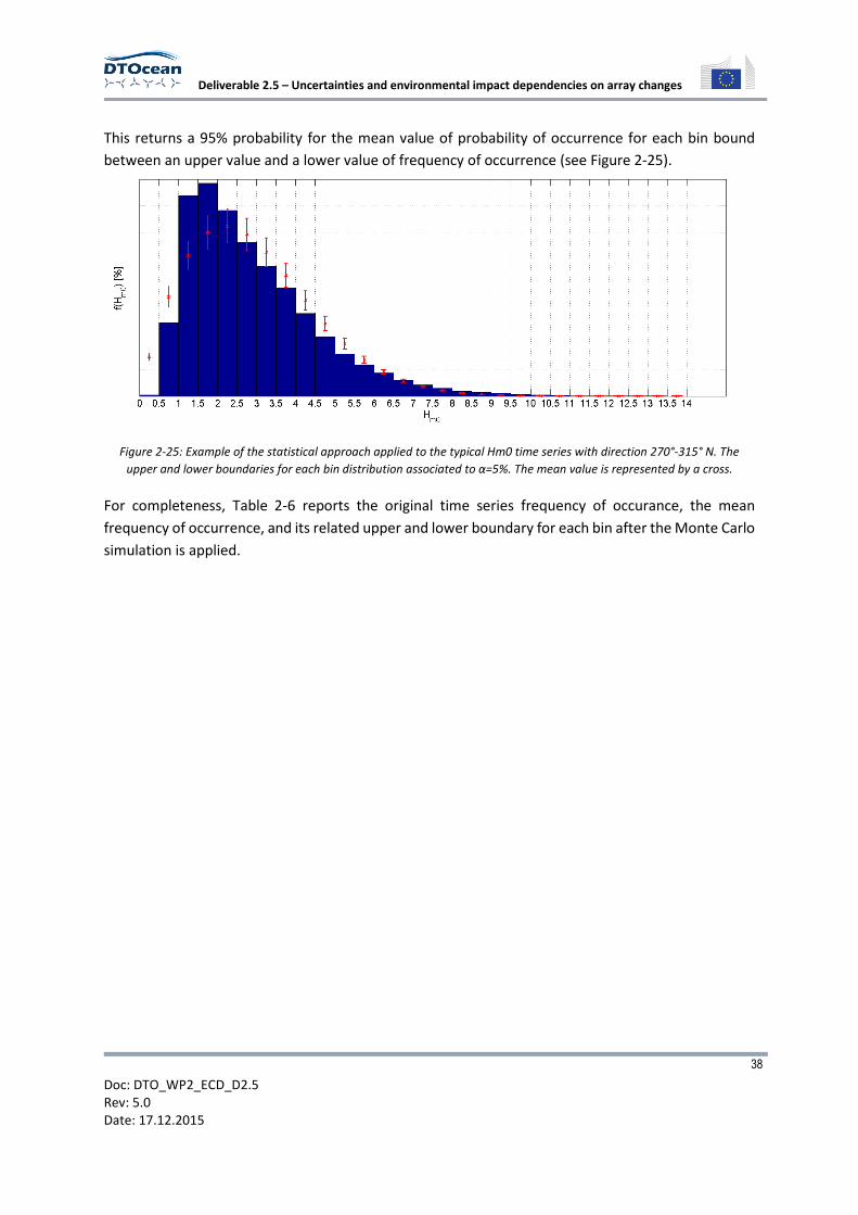
This returns a 95% probability for the mean value of probability of occurrence for each bin bound
between an upper value and a lower value of frequency of occurrence (see Figure 2-25).
Figure 2-25: Example of the statistical approach applied to the typical Hm0 time series with direction 270°-315° N. The
upper and lower boundaries for each bin distribution associated to α=5%. The mean value is represented by a cross.
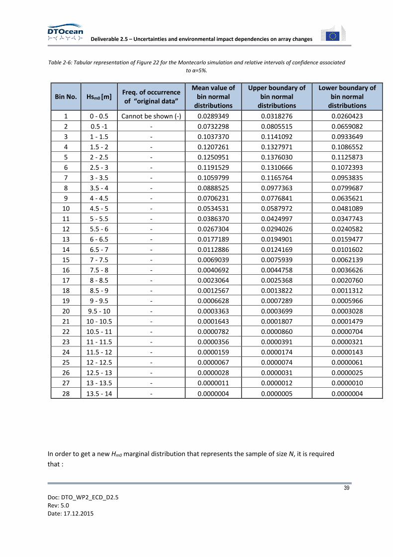
For completeness, Table 2-6 reports the original time series frequency of occurance, the mean
frequency of occurrence, and its related upper and lower boundary for each bin after the Monte Carlo
simulation is applied.
Deliverable 2.5 – Uncertainties and environmental impact dependencies on array changes
39
Doc: DTO_WP2_ECD_D2.5
Rev: 5.0
Date: 17.12.2015
Table 2-6: Tabular representation of Figure 22 for the Montecarlo simulation and relative intervals of confidence associated
to α=5%.
Bin No. Hsm0 [m] Freq. of occurrence
of “original data”
Mean value of
bin normal
distributions
Upper boundary of
bin normal
distributions
Lower boundary of
bin normal
distributions
1 0 - 0.5 Cannot be shown (-) 0.0289349 0.0318276 0.0260423
2 0.5 -1 - 0.0732298 0.0805515 0.0659082
3 1 - 1.5 - 0.1037370 0.1141092 0.0933649
4 1.5 - 2 - 0.1207261 0.1327971 0.1086552
5 2 - 2.5 - 0.1250951 0.1376030 0.1125873
6 2.5 - 3 - 0.1191529 0.1310666 0.1072393
7 3 - 3.5 - 0.1059799 0.1165764 0.0953835
8 3.5 - 4 - 0.0888525 0.0977363 0.0799687
9 4 - 4.5 - 0.0706231 0.0776841 0.0635621
10 4.5 - 5 - 0.0534531 0.0587972 0.0481089
11 5 - 5.5 - 0.0386370 0.0424997 0.0347743
12 5.5 - 6 - 0.0267304 0.0294026 0.0240582
13 6 - 6.5 - 0.0177189 0.0194901 0.0159477
14 6.5 - 7 - 0.0112886 0.0124169 0.0101602
15 7 - 7.5 - 0.0069039 0.0075939 0.0062139
16 7.5 - 8 - 0.0040692 0.0044758 0.0036626
17 8 - 8.5 - 0.0023064 0.0025368 0.0020760
18 8.5 - 9 - 0.0012567 0.0013822 0.0011312
19 9 - 9.5 - 0.0006628 0.0007289 0.0005966
20 9.5 - 10 - 0.0003363 0.0003699 0.0003028
21 10 - 10.5 - 0.0001643 0.0001807 0.0001479
22 10.5 - 11 - 0.0000782 0.0000860 0.0000704
23 11 - 11.5 - 0.0000356 0.0000391 0.0000321
24 11.5 - 12 - 0.0000159 0.0000174 0.0000143
25 12 - 12.5 - 0.0000067 0.0000074 0.0000061
26 12.5 - 13 - 0.0000028 0.0000031 0.0000025
27 13 - 13.5 - 0.0000011 0.0000012 0.0000010
28 13.5 - 14 - 0.0000004 0.0000005 0.0000004
In order to get a new Hm0 marginal distribution that represents the sample of size N, it is required
that :

Deliverable 2.5 – Uncertainties and environmental impact dependencies on array changes
40
Doc: DTO_WP2_ECD_D2.5
Rev: 5.0
Date: 17.12.2015
11
=∑=
Nb
kbink
f
Where kbinf is the frequency of occurrence of each bin. If the lower boundaries is a negative value,
then 0 has to be assumed as a lower boundary.
This allows not one unique combination, but all combinations of frequency of occurrence for each bin
within the CI bands that satisfies the equation above.
The new joint frequency of occurrence of Hm0 and Te can therefore be simply calculated as the product
of the two marginal distributions and a new scatter diagram is available to be fed to the WP2
hydrodynamic module.
For simplicity, the mean value column in Table 2-6 is chosen. Note also that the the summation of the
items in that column naturally sum up to 1.
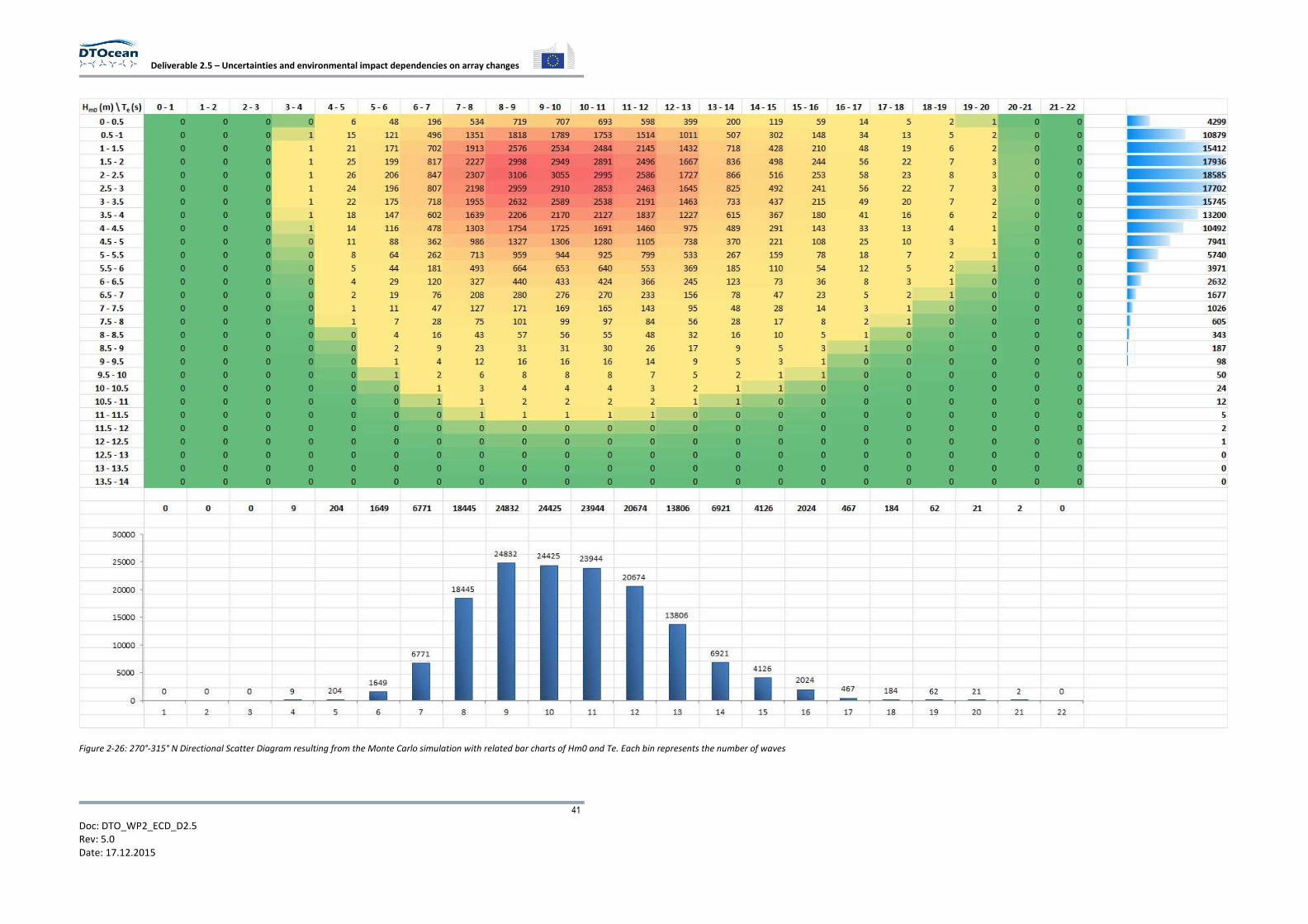
The new scatter diagram is therefore simply recalculated. Figure 2-26 shows the altered scatter
diagram expressed in frequency of occurrence (the total number N of waves will be the same as the
original).
Deliverable 2.5 – Uncertainties and environmental impact dependencies on array changes
41
Doc: DTO_WP2_ECD_D2.5
Rev: 5.0
Date: 17.12.2015
Figure 2-26: 270°-315° N Directional Scatter Diagram resulting from the Monte Carlo simulation with related bar charts of Hm0 and Te. Each bin represents the number of waves
Deliverable 2.5 – Uncertainties and environmental impact dependencies on array changes
42
Doc: DTO_WP2_ECD_D2.5
Rev: 5.0
Date: 17.12.2015
The hydrodynamic wave model can therefore be tested using a scatter diagram as input to the scatter
diagram shown in Figure 2-26.
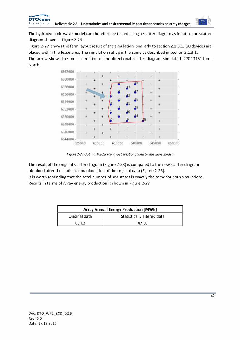
Figure 2-27 shows the farm layout result of the simulation. Similarly to section 2.1.3.1, 20 devices are
placed within the lease area. The simulation set up is the same as described in section 2.1.3.1.
The arrow shows the mean direction of the directional scatter diagram simulated, 270°-315° from
North.
Figure 2-27 Optimal WP2array layout solution found by the wave model.
The result of the original scatter diagram (Figure 2-28) is compared to the new scatter diagram
obtained after the statistical manipulation of the original data (Figure 2-26).
It is worth reminding that the total number of sea states is exactly the same for both simulations.
Results in terms of Array energy production is shown in Figure 2-28.
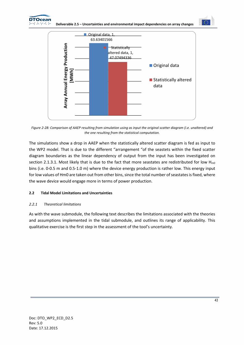
Array Annual Energy Production [MWh]
Original data Statistically altered data
63.63 47.07
Deliverable 2.5 – Uncertainties and environmental impact dependencies on array changes
43
Doc: DTO_WP2_ECD_D2.5
Rev: 5.0
Date: 17.12.2015
Figure 2-28: Comparison of AAEP resulting from simulation using as input the original scatter diagram (i.e. unaltered) and
the one resulting from the statistical computation.
The simulations show a drop in AAEP when the statistically altered scatter diagram is fed as input to
the WP2 model. That is due to the different “arrangement “of the seastets within the fixed scatter
diagram boundaries as the linear dependency of output from the input has been investigated on
section 2.1.3.1. Most likely that is due to the fact that more seastates are redistributed for low Hm0
bins (i.e. 0-0.5 m and 0.5-1.0 m) where the device energy production is rather low. This energy input
for low values of Hm0 are taken out from other bins, since the total number of seastates is fixed, where
the wave device would engage more in terms of power production.
2.2 Tidal Model Limitations and Uncertainties
2.2.1 Theoretical limitations
As with the wave submodule, the following text describes the limitations associated with the theories
and assumptions implemented in the tidal submodule, and outlines its range of applicability. This
qualitative exercise is the first step in the assessment of the tool’s uncertainty.
Original data, 1,
63.63401566
Statistically
altered data, 1,
47.07494336
Arr
ay
An
nu
al
En
erg
y P
rod
uct
ion
[MW
h]
Original data
Statistically altered
data
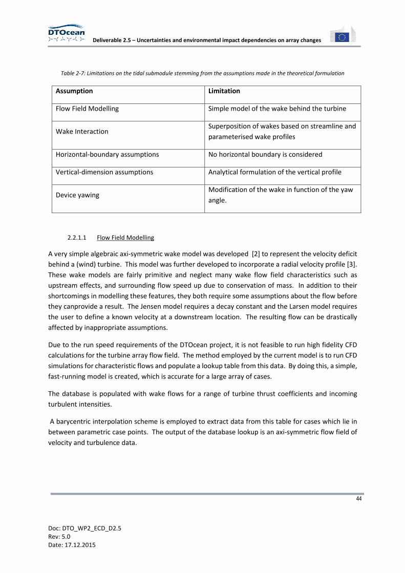
Deliverable 2.5 – Uncertainties and environmental impact dependencies on array changes
44
Doc: DTO_WP2_ECD_D2.5
Rev: 5.0
Date: 17.12.2015
Table 2-7: Limitations on the tidal submodule stemming from the assumptions made in the theoretical formulation
Assumption Limitation
Flow Field Modelling Simple model of the wake behind the turbine
Wake Interaction Superposition of wakes based on streamline and
parameterised wake profiles
Horizontal-boundary assumptions No horizontal boundary is considered
Vertical-dimension assumptions Analytical formulation of the vertical profile
Device yawing Modification of the wake in function of the yaw
angle.
2.2.1.1 Flow Field Modelling
A very simple algebraic axi-symmetric wake model was developed [2] to represent the velocity deficit
behind a (wind) turbine. This model was further developed to incorporate a radial velocity profile [3].
These wake models are fairly primitive and neglect many wake flow field characteristics such as
upstream effects, and surrounding flow speed up due to conservation of mass. In addition to their
shortcomings in modelling these features, they both require some assumptions about the flow before
they canprovide a result. The Jensen model requires a decay constant and the Larsen model requires
the user to define a known velocity at a downstream location. The resulting flow can be drastically
affected by inappropriate assumptions.
Due to the run speed requirements of the DTOcean project, it is not feasible to run high fidelity CFD
calculations for the turbine array flow field. The method employed by the current model is to run CFD
simulations for characteristic flows and populate a lookup table from this data. By doing this, a simple,
fast-running model is created, which is accurate for a large array of cases.
The database is populated with wake flows for a range of turbine thrust coefficients and incoming
turbulent intensities.
A barycentric interpolation scheme is employed to extract data from this table for cases which lie in
between parametric case points. The output of the database lookup is an axi-symmetric flow field of
velocity and turbulence data.
Deliverable 2.5 – Uncertainties and environmental impact dependencies on array changes
45
Doc: DTO_WP2_ECD_D2.5
Rev: 5.0
Date: 17.12.2015
This wake model, however, is not without its own limitations. The database is limited to looking up
points within its defined parameter space. There is no extrapolation algorithm. Thus for points outside
of the initial database definition, more points would need to be added to the database.
Another limitation of the database method is physical storage space. As points are added to the
database, or additional output variables are stored, the database will grow. Currently the database
stores stream-wise velocity and turbulence intensity over a spatial field of 20 by 4 turbine diameters.
With spatial discretization of 0.025D, the database takes up about 200Mb decompressed. This size will
scale linearly with an increased number of variables, discretization and domain size.
2.2.1.2 Wake interactions
The core of the wake interaction model is based on a rather simple Jensen model [10] to which the
parametric expression of the wake decay has been substituted with a CFD simulation based dataset
and which has been modified to follow streamlines composed of the wakes’ trajectories rather than
straight lines. Although these two additional features make the model less approximate than a
traditional Jensen model, it still has limitations in terms of applicability.
Several wake superimposition schemes will be tested during the model validation phase of this project
[13]. Nonetheless, the model, and thus wake interaction, cannot account for non-hydrostatic effects.
Consequently, the influences of turbines sitting in near wakes or upstream in the close vicinity of the
rotor will not be accurately modelled in the array’s performances and wake interactions. In practice
however, due to avoidance zones and maintenance ships safety requirements, such configurations are
unlikely to occur. Note that this theoretical limitation applies for both momentum and turbulence flow
characteristics.
From a hydrodynamics point of view, turbine wakes can be considered as stream tubes [14].
Accordingly, it has been assumed that a wake’s centre-lines follow the streamline generated at hub
locations in the initial flow. This assumption permits the model to account for the influence of the flow
advection on the wake expansion as well as to consider the distance between turbines relative to their
wake centre-line. Nevertheless, its numerical implementation may not work in highly rotational flows
with recurrent eddies. In practice however, such flows tend to be avoided as they would require
complex control of the machines as well as generated “chaotic” input to the drive train and hence
enhanced loading and fatigue to the entire converter.
Additionally, structure induced wakes are not accounted for in the present model. Device structure
may include a pile, nacelle, foundation, floating structure or any other component apart from the
blades themselves. This assumption may impact the overall energy balance assessment of the system
and wake interaction characterisation which, respectively, might introduce inaccuracy in modelled
impact and resource assessments.
Deliverable 2.5 – Uncertainties and environmental impact dependencies on array changes
46
Doc: DTO_WP2_ECD_D2.5
Rev: 5.0
Date: 17.12.2015
2.2.1.3 Horizontal-boundary assumptions
Lease’s horizontal/lateral boundaries/limits are considered open thus, as far as the model is
concerned, no horizontal boundary effects are accounted for nor modelled. This assumption may lead
to spurious results for configurations where the deployment is close to the edge of a constraint site
(such as a channel) or where the upstream row of the array layout densely covers the width of the
channel (e.g. approximately less than rotor-diameter lateral spacing between devices). In such cases,
blockage effects on the overall array performance will be under-estimated. Yet, in practice, considering
maintenance and environmental requirements, this type of configuration is likely to be avoided.
Whelan [15] developed a 1-d analytical solution for an infinite array permitting to investigate the
influence of the blockage effects on the percentage reduction in downstream free surface elevation.
Based on this model, it has been showed during the PerAWaT project that the downstream impact of
an infinite row of turbines at a lateral spacing of two rotor diameters can be considered negligible.
Yet this assumption seems valid only when the fluid is subcritical or tranquil, that is when the Froude
number Fr < 1, where
,- �.
/01
Nonetheless, and similarly to the current code, the previous example does not address the possibility
of upstream flow diversion away from the array and in situations where, for example, an array is
situated between an island and the main land, the upstream effect of the array should be considered
[15].
2.2.1.4 Vertical-dimension assumptions
The current model does not resolve the velocity vertical profile per se but assumes its shape based on
power-law formulas. Therefore, one should expect increased discrepancies in non-ideal sites with, for
instance, reverse shear and abnormal vertical stratification due steep density and/or temperature
gradients. In addition, wake influences on vertical profiles are not accounted for.
As discussed earlier and due to the open horizontal-boundary assumption, Whelan’s correction
method for blockage effects cannot be used in this model yet its Froude limit (i.e. Fr < 1) still applies.
Potential-flow approach should applied as suggested by the PerAWaT project [16]. However, for the
sake of computational time, a purely empirical approach has been chosen. Accordingly, based on
Sandia’s CFD model series of various vertical blockage ratios (i.e. rotor-diameter divided by the water
column height), either a Ct or wake-shape correction formula will be developed.
2.2.1.5 Device yawing
The current model accounts for yawing of devices from both the performance and wake points of view,
yet with two different approaches. The influence of yawing on performance is accounted for by
correcting the actuator disc surface area to be the “apparent” rotor surface area. This apparent surface

Deliverable 2.5 – Uncertainties and environmental impact dependencies on array changes
47
Doc: DTO_WP2_ECD_D2.5
Rev: 5.0
Date: 17.12.2015
can be defined as the projection of the actuator disc surface onto the plane perpendicular to the inflow
velocity vector. The influence of yawing however shall be accounted for in a similar fashion to the
vertical blockage effects, that is, through an empirical correction of the Ct and/or turbine diameter.
The axi-symmetric wake from the CFD database will be scaled in the span-wise direction to represent
the narrower cross section of a yawed turbine and the resulting narrower wake.
Consequently, in the case of performance, limitations will occur for turbines with ducted design and/or
yaw-specific control. In the case of the wake, the main assumption here is that the hydrodynamic
behaviour and relative shape of the wake shall stay the same and that only its dimensions would
change accordingly to Ct and/or turbine diameter. Extensive CFD simulations, experiments and/or in-
situ measurements are required to either infirm or confirm such assumptions.
2.2.2 Error analysis for validation
The ETI’s PerAWaT project produced results that could be used to evaluate the accuracy of the
methods used to account for blockage and turbulence intensity. The test plan therefore follows the
PerAWaT format. In particular in the following two cases will be compared.
1. 1 device
2. 2 devices at 1.5 D lateral spacing
The overall aim is to build up a validation dataset to assess the uncertainty of the DTOcean tidal model.
This will be done by running a number of cases in CFD and comparing these to the DTOcean tidal
module results and the available PerAWaT results.
2.2.2.1 PerAWaT flume experiments
The flume used in the PerAWaT experiments was a rectangular channel 5 meters wide by 12 meters
long and with a depth of 0.45 meters. It had a flat bottom and the first row of turbines was 6 meters
downstream of the inlet at mid-height in the water column Figure 2-29, Figure 2-30.
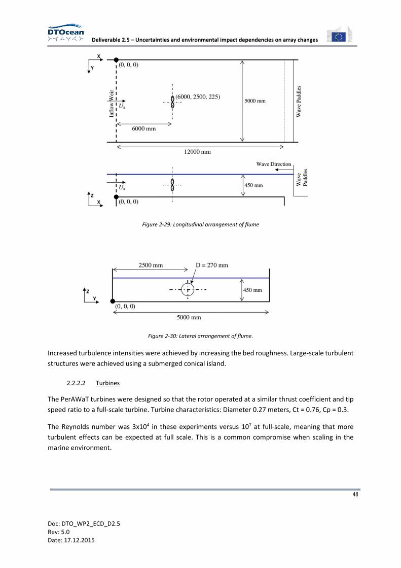
Deliverable 2.5 – Uncertainties and environmental impact dependencies on array changes
48
Doc: DTO_WP2_ECD_D2.5
Rev: 5.0
Date: 17.12.2015
Figure 2-29: Longitudinal arrangement of flume
Figure 2-30: Lateral arrangement of flume.
Increased turbulence intensities were achieved by increasing the bed roughness. Large-scale turbulent
structures were achieved using a submerged conical island.
2.2.2.2 Turbines
The PerAWaT turbines were designed so that the rotor operated at a similar thrust coefficient and tip
speed ratio to a full-scale turbine. Turbine characteristics: Diameter 0.27 meters, Ct = 0.76, Cp = 0.3.
The Reynolds number was 3x10⁴ in these experiments versus 107 at full-scale, meaning that more
turbulent effects can be expected at full scale. This is a common compromise when scaling in the
marine environment.
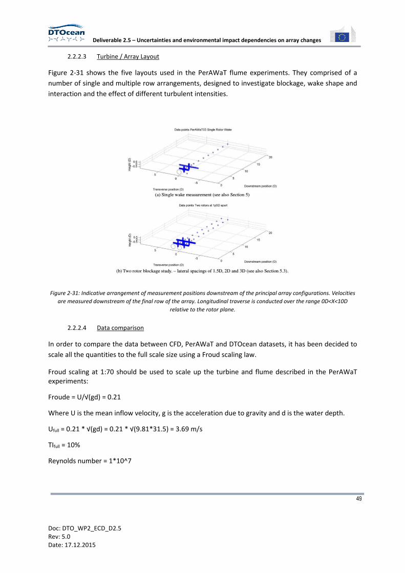
Deliverable 2.5 – Uncertainties and environmental impact dependencies on array changes
49
Doc: DTO_WP2_ECD_D2.5
Rev: 5.0
Date: 17.12.2015
2.2.2.3 Turbine / Array Layout
Figure 2-31 shows the five layouts used in the PerAWaT flume experiments. They comprised of a
number of single and multiple row arrangements, designed to investigate blockage, wake shape and
interaction and the effect of different turbulent intensities.
Figure 2-31: Indicative arrangement of measurement positions downstream of the principal array configurations. Velocities
are measured downstream of the final row of the array. Longitudinal traverse is conducted over the range 0D<X<10D
relative to the rotor plane.
2.2.2.4 Data comparison
In order to compare the data between CFD, PerAWaT and DTOcean datasets, it has been decided to
scale all the quantities to the full scale size using a Froud scaling law.
Froud scaling at 1:70 should be used to scale up the turbine and flume described in the PerAWaT
experiments:
Froude = U/√(gd) = 0.21
Where U is the mean inflow velocity, g is the acceleration due to gravity and d is the water depth.
Ufull = 0.21 * √(gd) = 0.21 * √(9.81*31.5) = 3.69 m/s
TIfull = 10%
Reynolds number = 1*10^7
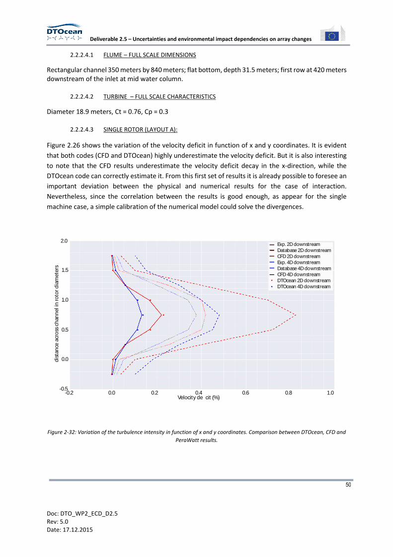
Deliverable 2.5 – Uncertainties and environmental impact dependencies on array changes
50
Doc: DTO_WP2_ECD_D2.5
Rev: 5.0
Date: 17.12.2015
2.2.2.4.1 FLUME – FULL SCALE DIMENSIONS
Rectangular channel 350 meters by 840 meters; flat bottom, depth 31.5 meters; first row at 420 meters
downstream of the inlet at mid water column.
2.2.2.4.2 TURBINE – FULL SCALE CHARACTERISTICS
Diameter 18.9 meters, Ct = 0.76, Cp = 0.3
2.2.2.4.3 SINGLE ROTOR (LAYOUT A):
Figure 2.26 shows the variation of the velocity deficit in function of x and y coordinates. It is evident
that both codes (CFD and DTOcean) highly underestimate the velocity deficit. But it is also interesting
to note that the CFD results underestimate the velocity deficit decay in the x-direction, while the
DTOcean code can correctly estimate it. From this first set of results it is already possible to foresee an
important deviation between the physical and numerical results for the case of interaction.
Nevertheless, since the correlation between the results is good enough, as appear for the single
machine case, a simple calibration of the numerical model could solve the divergences.
Figure 2-32: Variation of the turbulence intensity in function of x and y coordinates. Comparison between DTOcean, CFD and
PeraWatt results.
Exp. 2D downstreamDatabase 2D downstreamCFD 2D downstreamExp. 4D downstreamDatabase 4D downstreamCFD 4D downstreamDTOcean 2D downstreamDTOcean 4D downstream
Velocity de cit (%)
2.0
1.5
1.0
0.5
0.0
-0.5
dist
ance
acr
oss
chan
nel i
n ro
tor d
iam
eter
s
-0.2 0.0 0.2 0.4 0.6 0.8 1.0
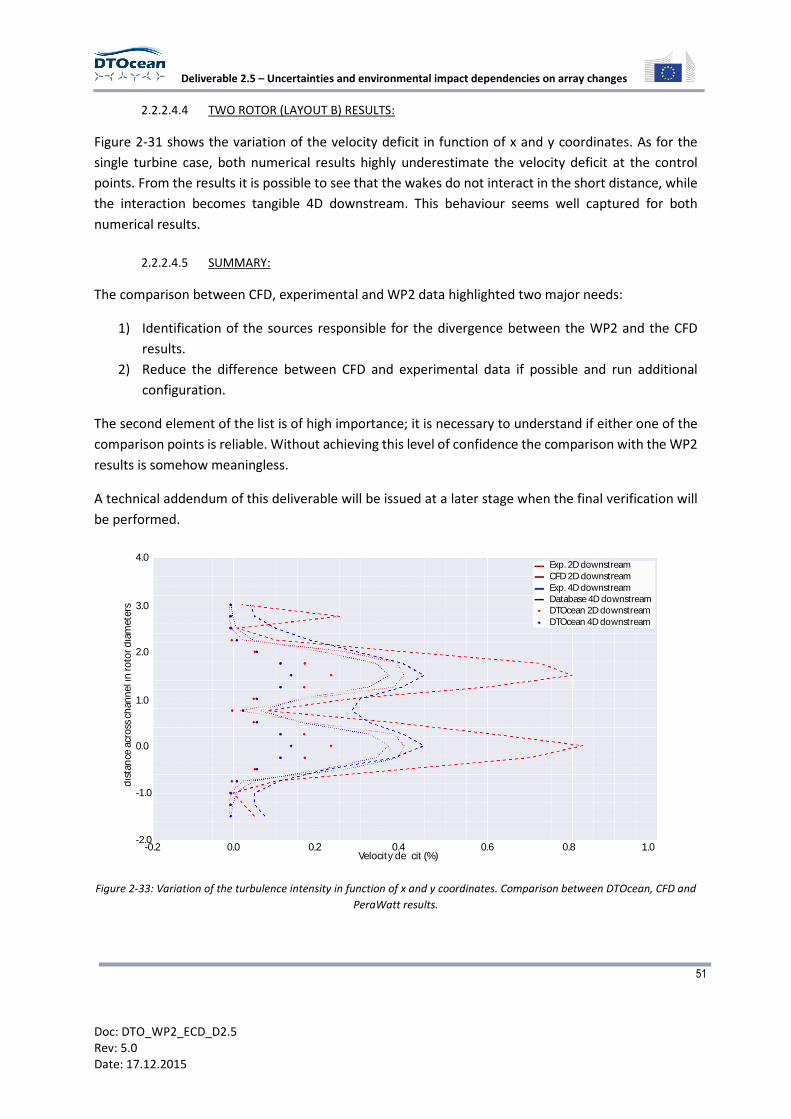
Deliverable 2.5 – Uncertainties and environmental impact dependencies on array changes
51
Doc: DTO_WP2_ECD_D2.5
Rev: 5.0
Date: 17.12.2015
2.2.2.4.4 TWO ROTOR (LAYOUT B) RESULTS:
Figure 2-31 shows the variation of the velocity deficit in function of x and y coordinates. As for the
single turbine case, both numerical results highly underestimate the velocity deficit at the control
points. From the results it is possible to see that the wakes do not interact in the short distance, while
the interaction becomes tangible 4D downstream. This behaviour seems well captured for both
numerical results.
2.2.2.4.5 SUMMARY:
The comparison between CFD, experimental and WP2 data highlighted two major needs:
1) Identification of the sources responsible for the divergence between the WP2 and the CFD
results.
2) Reduce the difference between CFD and experimental data if possible and run additional
configuration.
The second element of the list is of high importance; it is necessary to understand if either one of the
comparison points is reliable. Without achieving this level of confidence the comparison with the WP2
results is somehow meaningless.
A technical addendum of this deliverable will be issued at a later stage when the final verification will
be performed.
Figure 2-33: Variation of the turbulence intensity in function of x and y coordinates. Comparison between DTOcean, CFD and
PeraWatt results.
Exp. 2D downstreamCFD 2D downstreamExp. 4D downstreamDatabase 4D downstreamDTOcean 2D downstreamDTOcean 4D downstream
Velocity de cit (%)-0.2 0.0 0.2 0.4 0.6 0.8 1.0
4.0
3.0
2.0
1.0
0.0
-1.0
-2.0
dis
tanc
e ac
ross
cha
nnel
in ro
tor d
iam
eter
s
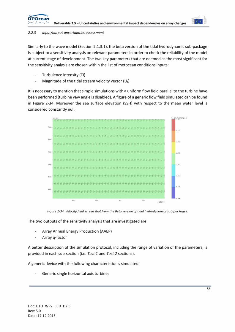
Deliverable 2.5 – Uncertainties and environmental impact dependencies on array changes
52
Doc: DTO_WP2_ECD_D2.5
Rev: 5.0
Date: 17.12.2015
2.2.3 Input/output uncertainties assessment
Similarly to the wave model (Section 2.1.3.1), the beta version of the tidal hydrodynamic sub-package
is subject to a sensitivity analysis on relevant parameters in order to check the reliability of the model
at current stage of development. The two key parameters that are deemed as the most significant for
the sensitivity analysis are chosen within the list of metocean conditions inputs:
- Turbulence intensity (TI)
- Magnitude of the tidal stream velocity vector (Ut)
It is necessary to mention that simple simulations with a uniform flow field parallel to the turbine have
been performed (turbine yaw angle is disabled). A figure of a generic flow field simulated can be found
in Figure 2-34. Moreover the sea surface elevation (SSH) with respect to the mean water level is
considered constantly null.
Figure 2-34: Velocity field screen shot from the Beta version of tidal hydrodynamics sub-packages.
The two outputs of the sensitivity analysis that are investigated are:
- Array Annual Energy Production (AAEP)
- Array q-factor
A better description of the simulation protocol, including the range of variation of the parameters, is
provided in each sub-section (i.e. Test 1 and Test 2 sections).
A generic device with the following characteristics is simulated:
- Generic single horizontal axis turbine;
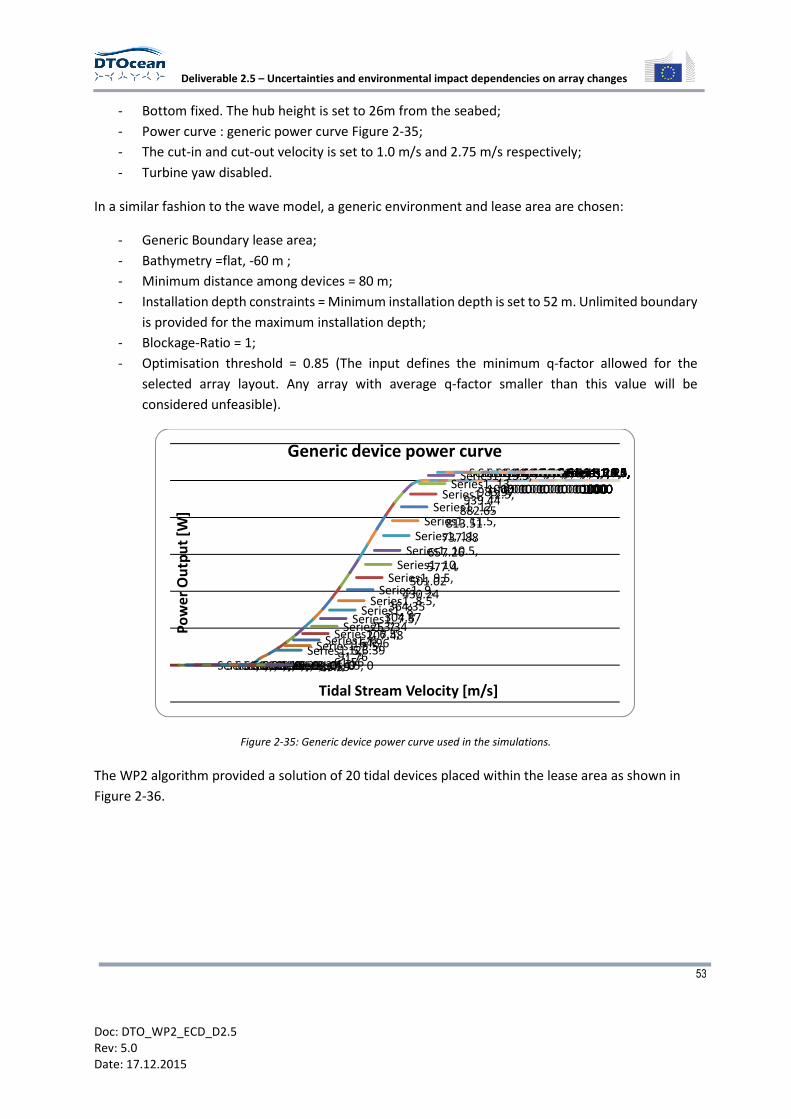
Deliverable 2.5 – Uncertainties and environmental impact dependencies on array changes
53
Doc: DTO_WP2_ECD_D2.5
Rev: 5.0
Date: 17.12.2015
- Bottom fixed. The hub height is set to 26m from the seabed;
- Power curve : generic power curve Figure 2-35;
- The cut-in and cut-out velocity is set to 1.0 m/s and 2.75 m/s respectively;
- Turbine yaw disabled.
In a similar fashion to the wave model, a generic environment and lease area are chosen:
- Generic Boundary lease area;
- Bathymetry =flat, -60 m ;
- Minimum distance among devices = 80 m;
- Installation depth constraints = Minimum installation depth is set to 52 m. Unlimited boundary
is provided for the maximum installation depth;
- Blockage-Ratio = 1;
- Optimisation threshold = 0.85 (The input defines the minimum q-factor allowed for the
selected array layout. Any array with average q-factor smaller than this value will be
considered unfeasible).
Figure 2-35: Generic device power curve used in the simulations.
The WP2 algorithm provided a solution of 20 tidal devices placed within the lease area as shown in
Figure 2-36.
Series1, 0, 0Series1, 0.5, 0Series1, 1, 0Series1, 1.5, 0Series1, 2, 0Series1, 2.5, 0Series1, 3, 0Series1, 3.5, 0Series1, 4, 0Series1, 4.5, 0
Series1, 5,
36.59
Series1, 5.5,
61.56
Series1, 6,
91.76
Series1, 6.5,
126.39
Series1, 7,
164.96
Series1, 7.5,
207.48
Series1, 8,
253.34
Series1, 8.5,
304.87
Series1, 9,
364.35
Series1, 9.5,
430.24
Series1, 10,
501.02
Series1, 10.5,
577.4
Series1, 11,
657.26
Series1, 11.5,
737.88
Series1, 12,
813.51
Series1, 12.5,
882.65
Series1, 13,
939.44
Series1, 13.5,
983.97
Series1, 14,
1000
Series1, 14.5,
1000
Series1, 15,
1000
Series1, 15.5,
1000
Series1, 16,
1000
Series1, 16.5,
1000
Series1, 17,
1000
Series1, 17.5,
1000
Series1, 18,
1000
Series1, 18.5,
1000
Series1, 19,
1000
Series1, 19.5,
1000
Series1, 20,
1000
Series1, 20.5,
1000
Series1, 21,
1000
Series1, 21.5,
1000
Series1, 22,
1000
Series1, 22.5,
1000
Series1, 23,
1000
Series1, 23.5,
1000
Series1, 24,
1000
Series1, 24.5,
1000
Series1, 25,
1000
Po
we
r O
utp
ut
[W]
Tidal Stream Velocity [m/s]
Generic device power curve
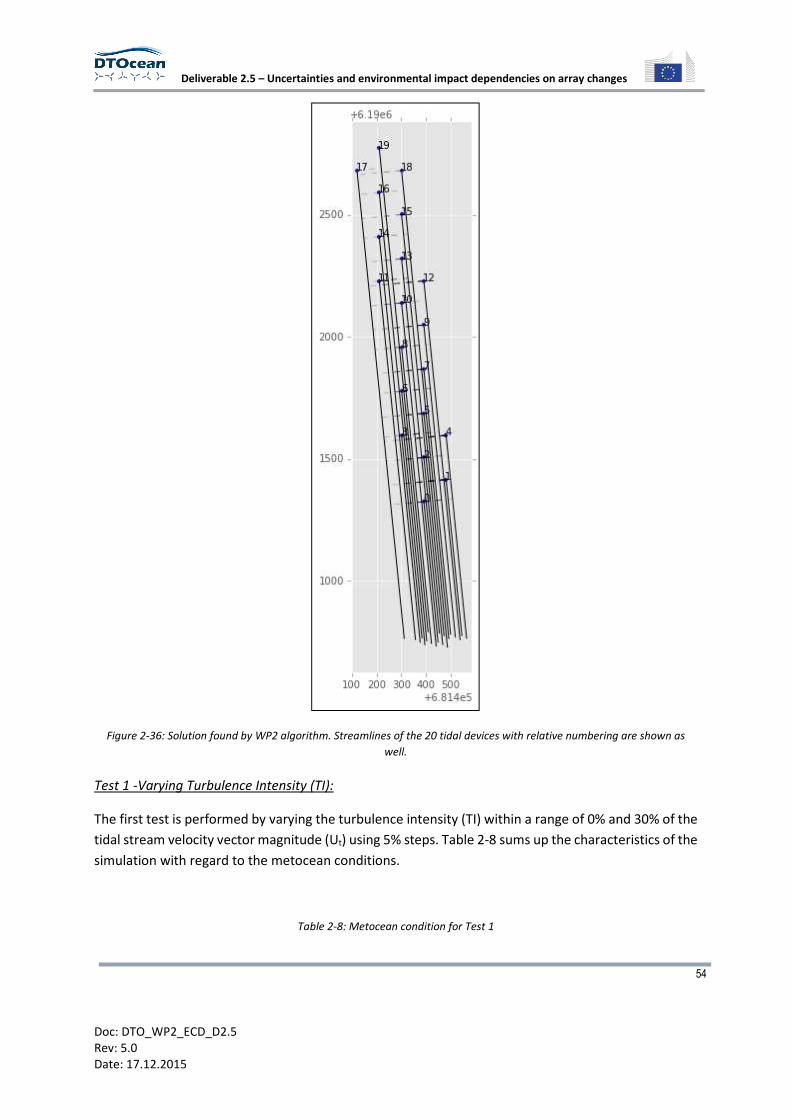
Deliverable 2.5 – Uncertainties and environmental impact dependencies on array changes
54
Doc: DTO_WP2_ECD_D2.5
Rev: 5.0
Date: 17.12.2015
Figure 2-36: Solution found by WP2 algorithm. Streamlines of the 20 tidal devices with relative numbering are shown as
well.
Test 1 -Varying Turbulence Intensity (TI):
The first test is performed by varying the turbulence intensity (TI) within a range of 0% and 30% of the
tidal stream velocity vector magnitude (Ut) using 5% steps. Table 2-8 sums up the characteristics of the
simulation with regard to the metocean conditions.
Table 2-8: Metocean condition for Test 1
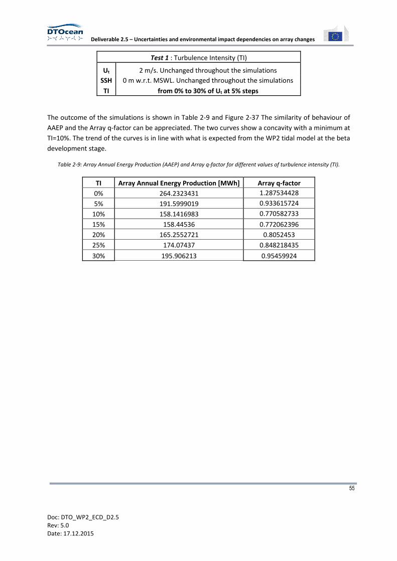
Deliverable 2.5 – Uncertainties and environmental impact dependencies on array changes
55
Doc: DTO_WP2_ECD_D2.5
Rev: 5.0
Date: 17.12.2015
Test 1 : Turbulence Intensity (TI)
Ut 2 m/s. Unchanged throughout the simulations
SSH 0 m w.r.t. MSWL. Unchanged throughout the simulations
TI from 0% to 30% of Ut at 5% steps
The outcome of the simulations is shown in Table 2-9 and Figure 2-37 The similarity of behaviour of
AAEP and the Array q-factor can be appreciated. The two curves show a concavity with a minimum at
TI=10%. The trend of the curves is in line with what is expected from the WP2 tidal model at the beta
development stage.
Table 2-9: Array Annual Energy Production (AAEP) and Array q-factor for different values of turbulence intensity (TI).
TI Array Annual Energy Production [MWh] Array q-factor
0% 264.2323431 1.287534428
5% 191.5999019 0.933615724
10% 158.1416983 0.770582733
15% 158.44536 0.772062396
20% 165.2552721 0.8052453
25% 174.07437 0.848218435
30% 195.906213 0.95459924
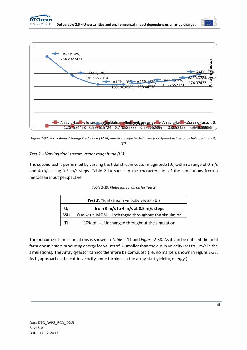
Deliverable 2.5 – Uncertainties and environmental impact dependencies on array changes
56
Doc: DTO_WP2_ECD_D2.5
Rev: 5.0
Date: 17.12.2015
Figure 2-37: Array Annual Energy Production (AAEP) and Array q-factor behavior for different values of turbulence intensity
(TI).
Test 2 – Varying tidal stream vector magnitude (Ut):
The second test is performed by varying the tidal stream vector magnitude (Ut) within a range of 0 m/s
and 4 m/s using 0.5 m/s steps. Table 2-10 sums up the characteristics of the simulations from a
metocean input perspective.
Table 2-10: Metocean condition for Test 2
Test 2: Tidal stream velocity vector (Ut)
Ut from 0 m/s to 4 m/s at 0.5 m/s steps
SSH 0 m w.r.t. MSWL. Unchanged throughout the simulation
TI 10% of Ut . Unchanged throughout the simulation
The outcome of the simulations is shown in Table 2-11 and Figure 2-38. As it can be noticed the tidal
farm doesn’t start producing energy for values of Ut smaller than the cut-in velocity (set to 1 m/s in the
simulations). The Array q-factor cannot therefore be computed (i.e. no markers shown in Figure 2-38.
As Ut approaches the cut-in velocity some turbines in the array start yielding energy (
AAEP, 0%,
264.2323431
AAEP, 5%,
191.5999019AAEP, 10%,
158.1416983
AAEP, 15%,
158.44536
AAEP, 20%,
165.2552721
AAEP, 25%,
174.07437
AAEP, 30%,
195.906213
Array q-factor, 1,
1.287534428
Array q-factor, 2,
0.933615724
Array q-factor, 3,
0.770582733
Array q-factor, 4,
0.772062396
Array q-factor, 5,
0.8052453
Array q-factor, 6,
0.848218435
Array q-factor, 7,
0.95459924
Arr
ay
q-f
act
or
Turbulence IntensityAAEP Array q-factor
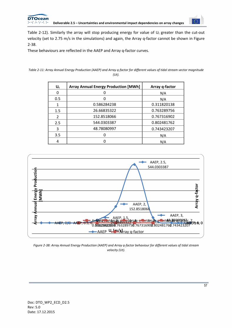
Deliverable 2.5 – Uncertainties and environmental impact dependencies on array changes
57
Doc: DTO_WP2_ECD_D2.5
Rev: 5.0
Date: 17.12.2015
Table 2-12). Similarly the array will stop producing energy for value of Ut greater than the cut-out
velocity (set to 2.75 m/s in the simulations) and again, the Array q-factor cannot be shown in Figure
2-38.
These behaviours are reflected in the AAEP and Array q-factor curves.
Table 2-11: Array Annual Energy Production (AAEP) and Array q-factor for different values of tidal stream vector magnitude
(Ut).
Ut Array Annual Energy Production [MWh] Array q-factor
0 0 N/A
0.5 0 N/A
1 0.586284238 0.311820138
1.5 26.66835322 0.763289756
2 152.8518066 0.767316902
2.5 544.0303387 0.802481762
3 48.78080997 0.743423207
3.5 0 N/A
4 0 N/A
Figure 2-38: Array Annual Energy Production (AAEP) and Array q-factor behaviour for different values of tidal stream
velocity (Ut).
AAEP, 0, 0 AAEP, 0.5, 0AAEP, 1,
0.586284238
AAEP, 1.5,
26.66835322
AAEP, 2,
152.8518066
AAEP, 2.5,
544.0303387
AAEP, 3,
48.78080997AAEP, 3.5, 0AAEP, 4, 0
Array q-factor, 3,
0.311820138
Array q-factor, 4,
0.763289756
Array q-factor, 5,
0.767316902
Array q-factor, 6,
0.802481762
Array q-factor, 7,
0.743423207
Arr
ay
q-f
act
or
Arr
ay
An
nu
al
En
erg
y P
rod
uct
ion
[MW
h]
Ut [m/s]AAEP Array q-factor
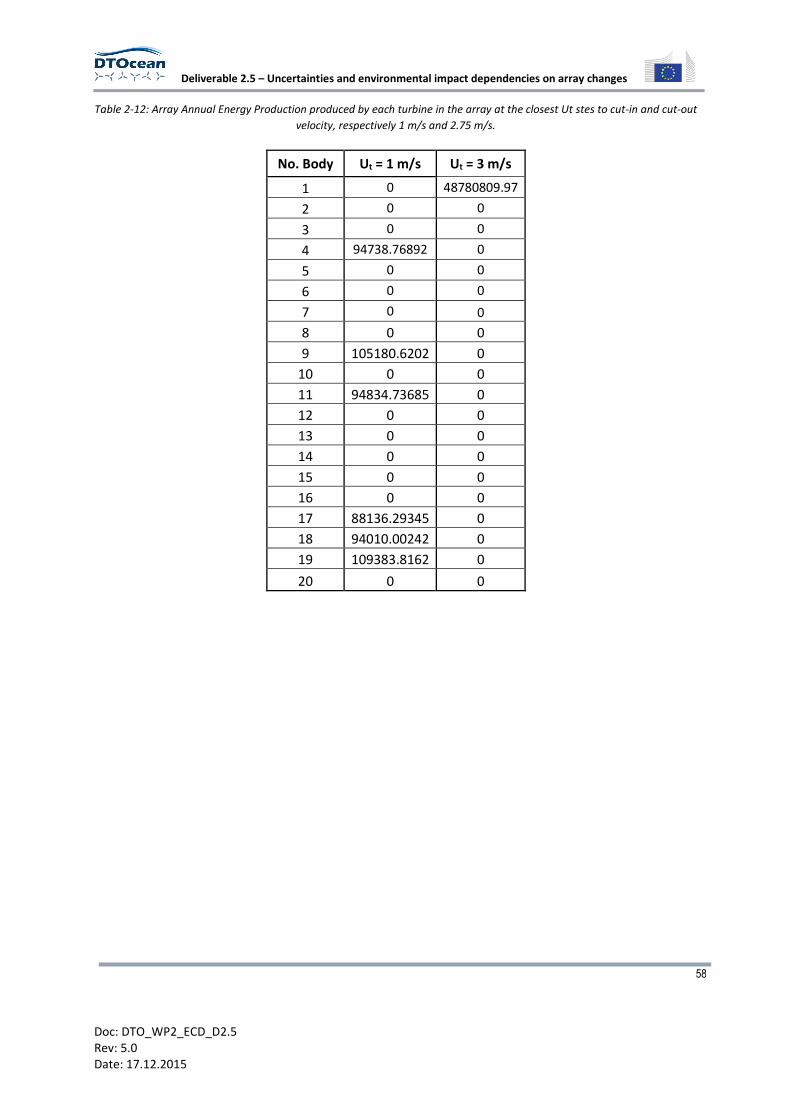
Deliverable 2.5 – Uncertainties and environmental impact dependencies on array changes
58
Doc: DTO_WP2_ECD_D2.5
Rev: 5.0
Date: 17.12.2015
Table 2-12: Array Annual Energy Production produced by each turbine in the array at the closest Ut stes to cut-in and cut-out
velocity, respectively 1 m/s and 2.75 m/s.
No. Body Ut = 1 m/s Ut = 3 m/s
1 0 48780809.97
2 0 0
3 0 0
4 94738.76892 0
5 0 0
6 0 0
7 0 0
8 0 0
9 105180.6202 0
10 0 0
11 94834.73685 0
12 0 0
13 0 0
14 0 0
15 0 0
16 0 0
17 88136.29345 0
18 94010.00242 0
19 109383.8162 0
20 0 0
Deliverable 2.5 – Uncertainties and environmental impact dependencies on array changes
59
Doc: DTO_WP2_ECD_D2.5
Rev: 5.0
Date: 17.12.2015
3 INTRODUCTION TO THE ENVIRONMENTAL ISSUES RELATED TO ARRAY DESIGN
Specifications of environmental conditions and dependencies on array changes can generate
uncertainties in power production. Indeed, deployment of wave and tidal arrays can alter the hydraulic
environment and change the amount of resource available for extraction. Such deployments also have
impacts in terms of environmental issues.
Within the framework of DTOcean, a specific module, called the Environmental Impact Assessment
Module (EIAM), is designed to assess the environmental impacts of the various technological choices
made to optimize an array of wave or tidal devices.
The following chapter of this document deals specifically with the impacts of the introduction of
devices in the marine environment in term of hydrodynamics and array optimization. In that context,
several environmental impacts have been selected. The first environmental concern regards the
amount of energy extracted by arrays and the direct consequences on the surrounding waters with
modification of the flow. Another concern is the modification water turbidity that might directly affect
primary production rates, sediment transport and benthic habitats. Noise is also a major
environmental concern, especially at array levels. Array optimization and changes will also have major
implications in terms of collision risks for marine life. Chemical pollution risks are also a concern with
such deployments. Finally, some factors such as reef effects, reserve effects and resting places can be
considered beneficial and are also dependent on array choices.
In this report, all the issues cited above are summarized in terms of potential environmental impact.
Some general recommendations to minimize environmental effects and specific recommendations
based on choices driven by hydrodynamic concerns are also given. Finally, the last section of this
document gives a description of each environmental issue and its potential impacts, and of the
developed EIAM functions with detailed explanations of calibration choices and values.
4 MAIN ENVIRONMENTAL ISSUES ASSOCIATED TO ARRAY CHANGES
4.1 Environmental background
4.1.1 Energy extraction
Tidal and wave marine energy converter devices operate by using the kinetic energy provided by
currents and waves, respectively. This is often done using a turbine unit that will extract energy from
the surrounding environment possibly resulting (at least for tidal energy converters) in changes in the
water column velocity structure [17]. The flow upstream of a device will be decelerated, and a
turbulent wake with a reduction of velocity will appear downstream the device [18]. An acceleration
of flow around the device will also usually result. These modifications will directly affect the
resuspension, and accumulation of sediment. Overall, the water flow remains a major process of the
repartition of species in the water column and any changes can have an effect on marine ecosystems
[19]. All sort of habitat can be impacted as shown in the Figure 4-1 which highlights marine habitats
which may be altered by a change of the hydrodynamic flow [19].
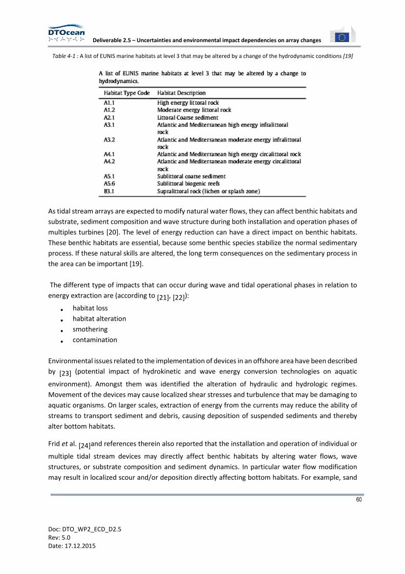
Deliverable 2.5 – Uncertainties and environmental impact dependencies on array changes
60
Doc: DTO_WP2_ECD_D2.5
Rev: 5.0
Date: 17.12.2015
Table 4-1 : A list of EUNIS marine habitats at level 3 that may be altered by a change of the hydrodynamic conditions [19]
As tidal stream arrays are expected to modify natural water flows, they can affect benthic habitats and
substrate, sediment composition and wave structure during both installation and operation phases of
multiples turbines [20]. The level of energy reduction can have a direct impact on benthic habitats.
These benthic habitats are essential, because some benthic species stabilize the normal sedimentary
process. If these natural skills are altered, the long term consequences on the sedimentary process in
the area can be important [19].
The different type of impacts that can occur during wave and tidal operational phases in relation to
energy extraction are (according to [21], [22]):
• habitat loss
• habitat alteration
• smothering
• contamination
Environmental issues related to the implementation of devices in an offshore area have been described
by [23] (potential impact of hydrokinetic and wave energy conversion technologies on aquatic
environment). Amongst them was identified the alteration of hydraulic and hydrologic regimes.
Movement of the devices may cause localized shear stresses and turbulence that may be damaging to
aquatic organisms. On larger scales, extraction of energy from the currents may reduce the ability of
streams to transport sediment and debris, causing deposition of suspended sediments and thereby
alter bottom habitats.
Frid et al. [24]and references therein also reported that the installation and operation of individual or
multiple tidal stream devices may directly affect benthic habitats by altering water flows, wave
structures, or substrate composition and sediment dynamics. In particular water flow modification
may result in localized scour and/or deposition directly affecting bottom habitats. For example, sand
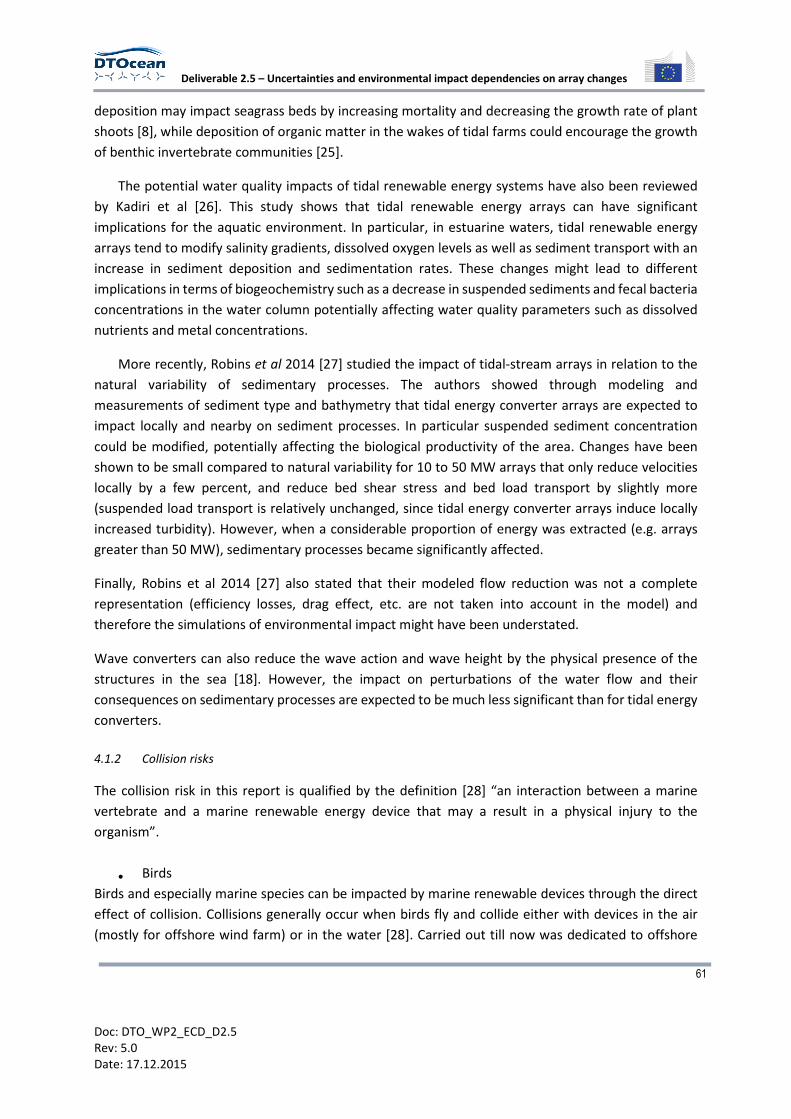
Deliverable 2.5 – Uncertainties and environmental impact dependencies on array changes
61
Doc: DTO_WP2_ECD_D2.5
Rev: 5.0
Date: 17.12.2015
deposition may impact seagrass beds by increasing mortality and decreasing the growth rate of plant
shoots [8], while deposition of organic matter in the wakes of tidal farms could encourage the growth
of benthic invertebrate communities [25].
The potential water quality impacts of tidal renewable energy systems have also been reviewed
by Kadiri et al [26]. This study shows that tidal renewable energy arrays can have significant
implications for the aquatic environment. In particular, in estuarine waters, tidal renewable energy
arrays tend to modify salinity gradients, dissolved oxygen levels as well as sediment transport with an
increase in sediment deposition and sedimentation rates. These changes might lead to different
implications in terms of biogeochemistry such as a decrease in suspended sediments and fecal bacteria
concentrations in the water column potentially affecting water quality parameters such as dissolved
nutrients and metal concentrations.
More recently, Robins et al 2014 [27] studied the impact of tidal-stream arrays in relation to the
natural variability of sedimentary processes. The authors showed through modeling and
measurements of sediment type and bathymetry that tidal energy converter arrays are expected to
impact locally and nearby on sediment processes. In particular suspended sediment concentration
could be modified, potentially affecting the biological productivity of the area. Changes have been
shown to be small compared to natural variability for 10 to 50 MW arrays that only reduce velocities
locally by a few percent, and reduce bed shear stress and bed load transport by slightly more
(suspended load transport is relatively unchanged, since tidal energy converter arrays induce locally
increased turbidity). However, when a considerable proportion of energy was extracted (e.g. arrays
greater than 50 MW), sedimentary processes became significantly affected.
Finally, Robins et al 2014 [27] also stated that their modeled flow reduction was not a complete
representation (efficiency losses, drag effect, etc. are not taken into account in the model) and
therefore the simulations of environmental impact might have been understated.
Wave converters can also reduce the wave action and wave height by the physical presence of the
structures in the sea [18]. However, the impact on perturbations of the water flow and their
consequences on sedimentary processes are expected to be much less significant than for tidal energy
converters.
4.1.2 Collision risks
The collision risk in this report is qualified by the definition [28] “an interaction between a marine
vertebrate and a marine renewable energy device that may a result in a physical injury to the
organism”.
• Birds
Birds and especially marine species can be impacted by marine renewable devices through the direct
effect of collision. Collisions generally occur when birds fly and collide either with devices in the air
(mostly for offshore wind farm) or in the water [28]. Carried out till now was dedicated to offshore
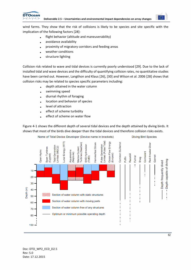
Deliverable 2.5 – Uncertainties and environmental impact dependencies on array changes
62
Doc: DTO_WP2_ECD_D2.5
Rev: 5.0
Date: 17.12.2015
wind farms. They show that the risk of collisions is likely to be species and site specific with the
implication of the following factors [28]:
• flight behavior (altitude and maneuverability)
• avoidance availability
• proximity of migratory corridors and feeding areas
• weather conditions
• structure lighting
Collision risk related to wave and tidal devices is currently poorly understood [29]. Due to the lack of
installed tidal and wave devices and the difficulty of quantifying collision rates, no quantitative studies
have been carried out. However, Langthon and Klaus [26], [30] and Wilson et al. 2006 [28] shows that
collision risks may be related to species specific parameters including:
• depth attained in the water column
• swimming speed
• diurnal rhythm of foraging
• location and behavior of species
• level of attraction
• effect of scheme turbidity
• effect of scheme on water flow
Figure 4-1 shows the different depth of several tidal devices and the depth attained by diving birds. It
shows that most of the birds dive deeper than the tidal devices and therefore collision risks exists.

Deliverable 2.5 – Uncertainties and environmental impact dependencies on array changes
63
Doc: DTO_WP2_ECD_D2.5
Rev: 5.0
Date: 17.12.2015
Figure 4-1 :Turbine depths and diving depths of bird species [31].
A few data are available on collision risks between birds and submerged structures other than offshore
wind devices [31]. Grecian et al 2010 [32] indicate that there is a link between the type of device and
the behavior of diving birds. The following factors affect the risk of collision:
• type of devices (floating or fixed)
• moving part of device (blades, cables)
• depth of device
• Static structure
• horizontal device
• vertical device
According to Grecian et al 2010 [32], the risk of collision between birds and wave devices may be low
during flights because wave-powered devices have a small profile outside the water. However, this
study highlights the fact that the collision risk is also dependent of several parameters such as:
• bad weather
• reduced visibility
• state of sea
• tide conditions
• Marine mammals
As with birds, marine mammals may be affected by MRE devices, particularly in term of collision and
entanglement with tidal and wave devices. European waters are populated by a substantial number of
marine mammals including seals and cetaceans. To date, a substantial amount of studies examining
the potential impacts of MRE on marine mammals have been carried out, see for example [33], [22],
[34], and [35].
Overall the risk of collision is a function of species, body size, swimming behavior and skills, capacity
to detect devices as well as device type. The design of devices is also an important factor with regards
to collisions. Many devices have a large surface structure and some trap points (ducts, vent devices,
floating boxes etc.). Each of these elements can be dangerous for mammals and raise the risk of
collision. Inger et al. (2009) [36] indicates that rotating devices from wave and tidal technologies may
lead to injury or death.
In conjunction with mammal behavior, the organization of devices in an array as well as the location
of the array itself are also important. Collision risks will be depending on depths, array organizations
(devices in parallel, series) or location (narrow channels, open waters, sounds, etc). According to
Wilson et al 2006 [28], the placing of structures may produce confusion and therefore a behavior
modification. The detection of devices by mammals that do not have acoustic detection abilities (or
mechanoreceptors) can be affected in highly turbid waters during storm events. Furthermore, large

Deliverable 2.5 – Uncertainties and environmental impact dependencies on array changes
64
Doc: DTO_WP2_ECD_D2.5
Rev: 5.0
Date: 17.12.2015
mammals like whales appear to be more vulnerable than smaller species due to their size and bulk
[35], [22]. The age of a mammal has been shown to also be a factor of risk as a preponderance of
juveniles is noticed in entanglement observations, probably due to their lack of experience [35], [22]
However, as highlighted [19] there is still a high level of uncertainty regarding whether collision risks
might impact mammals at population level. Most of the studies carried out to date are based on model
predictions. For example Wilson et al (2006) [28] indicates a prediction of encounter rate of 13
individuals per year per turbine in an area surrounding a commercial deployment on the west coast of
Scotland. Carter et al. [37] also modelled the likely encounter rate of marine mammals with marine
energy devices and concluded that there is a possible risk for marine mammals only in case of big
devices (diameter around 15 to 20 m). Nevertheless, Keenan et al. (2011) [38] showed that no major
impacts on marine mammals have been detected across the 3 years of post-installation monitoring of
the SeaGen turbine installed in the Narrows of Strangford Lough (Northern Ireland).
4.1.3 Turbidity
Turbidity is the cloudiness or haziness of a fluid caused by large numbers of individual particles.
It usually gives an indication of the concentration of suspended particles in water.
MRE developments can modify the turbidity of ecosystems, especially during construction phases,
while some activities involve interaction with the sediment. Thus, the concentration of re suspended
particulate matter (SPM) can substantially increase locally. During operational phases, higher
concentrations of SPM exceeding the natural variability can occur when tidal currents exceed a certain
velocity [39] due to the interaction of the current with devices.
The main environmental impact generated by turbid waters is the adsorption of the light that may limit
primary production. Indeed, light attenuation by suspended sediments confines the photic zone to a
small fraction of the water column, such that light limitation is a major control on phytoplankton
production and turnover rate [40].
Turbid waters can also impact benthos animals like filter-feeders and impact the development and
growth of different species. SPM concentration increases can cause a decrease in respiration (due to
clogging of filtration mechanisms), a behavioral alteration of species and a risk for eggs and larvae [41].
Such impacts are identified in high turbidity due to dredging activity. In contrast, the impact of an
increase in turbidity on other species like marine mammals or birds is poorly known. Marine mammals
often reside in turbid waters, so significant impacts from turbidity are improbable [41]. However, high
turbidities may impact the ability to hunt, and the visual resolution power of diving-birds [42], [41].
Finally, turbid waters can generate high sedimentation rates (often locally) in areas where
hydrodynamic conditions are more favorable, thus changing the sediment structure and the associated
benthic communities. In general, regularly disturbed habitats characterized by fine sands and fast-

Deliverable 2.5 – Uncertainties and environmental impact dependencies on array changes
65
Doc: DTO_WP2_ECD_D2.5
Rev: 5.0
Date: 17.12.2015
growing opportunistic species are less affected, and recover quicker, than stable habitats monopolized
by coarse gravels and slow-growing sessile fauna and flora [43]. In addition to changing community
structure, sediment deposition can smother or bury marine organisms associated with the seabed.
Non-mobile organisms and early life stages that are unable to move are most at risk [41].
4.1.4 Underwater noise
The quantification of underwater noise due to wave and tidal devices is poorly known. Underwater
noise is device specific and also directly related to the number of devices. Each device has a range of
associated noise spectra [44]. Sources of noise are multiple. They have been listed by Robinson et al
[44] as:
• Noise generated by turbulence and vortex shedding
• Noise from hydraulics, joints and hinges
• Noise from moorings
• Impact of surface waves
• Rotating machinery
• Movement of air or water
• Noise in all operational modes (start-up, braking, stationary)
Noise radiation is created by the moving parts of devices. This movement generates different pressure
and turbulence. The variety of designs can then produce a large range of potential noise that can
propagate in the water column.
The decibel level of sound is stated in the form of the dB re 1 µPa. The µPa is a unit of pressure [45].
There are different levels of reference to define the underwater noise. The SPL: is the expression of
the Sound Pressure Level in decibel (dB). The SEL: Sound Exposure Level metric, sums the acoustic
energy over a measurement period, and effectively takes account both the SPL and the duration of the
sound in the acoustic environment [46].
Environmental effects related to noise are expected to impact the marine life in different ways. Marine
mammals, for example, can adapt to a wide variety of natural sound and have adaptive mechanisms
to deal with many anthropogenic sounds. The frequencies that can be heard from marine mammals
range from less than 100 Hz up to 180 kHz, making predictions of potential effects challenging.
However, when anthropogenic sounds are excessive in level, frequency or even duration, they might
exceed the mammal’s adaptive capacity and cause the following main effects (see [47] and reference
therein):
• Physical injuries: with permanent threshold shifts or loss of hearing sensitivity resulting from
either a brief exposure to very intense sounds or a longer duration to moderately intense

Deliverable 2.5 – Uncertainties and environmental impact dependencies on array changes
66
Doc: DTO_WP2_ECD_D2.5
Rev: 5.0
Date: 17.12.2015
sounds, or intermittently but repeatedly to sounds sufficient to cause temporary threshold
shifts [48]
• Physiological Reactions: with sound exposure that causes non-auditory physiological effects
like stress.
• Masking: when sounds are more difficult to hear because of added noise affecting mammal's
detection and interpretation. Masking may affect (1) reproduction if a female cannot hear
potential males vocalizing, (2) mother-offspring bonding and recognition if the pair cannot
communicate effectively, (3) foraging if animals that hunt cooperatively cannot communicate
or if they cannot detect prey , and (4) survival if an animal cannot detect predators or other
threats.
• Behavioral responses: following the detection of sounds, mammals can change habitat use to
avoid areas of higher sound levels or modify patterns such as diving and surfacing or vocalizing.
As with mammals, fish are characterized by a wide range of hearing structures, resulting in different
capacities and sensitivities to noise. They use biological noise to gain information about their
surrounding environment in order to locate their prey and predators or even communicate. Noise may
generate physical injury, hearing loss and behavioral changes. However, the impact is unknown and
will be dependent on the received sound. In their paper review on several European fishes, Gill and
Bartlett [49] indicated that fishes that receive high intensity sound pressures (e.g. close proximity to
MRE construction) may be negatively be impacted to some degree, whereas those at distances of 100s
to 1000s of meters may exhibit behavior responses. During operation there may be more subtle
behavioral effects that should be considered over the life time of the MRE development. Slabbekoorn
et al. 2010 [50] also stated that very loud sounds of relatively short duration can harm nearby fish.
For birds, noise is considered as an indirect effect. Indeed it may cause a reduction in fish abundance
and therefore reduce food resources. For both mammals and fish, displacement is also another
potential effect generated by noise where devices are deployed, but this effect is hardly quantifiable.
Different kinds of noise will be generated during construction/installation and operation. However, the
construction/installation phase is usually of particular concern due to specific activities such as
anchoring and especially pile driving. On that matter and in the absence of large tidal and wave
developments, most of the studies carried out on noise are related to wind farms. Bailey et al. 2010
[51] measured pile driving noise at distances of 0.1 km (maximum broadband peak to peak sound level
205 dB re 1 µPa) to 80 km (no longer distinguishable above background noise). These sound levels
were related to noise exposure criteria for marine mammals to assess possible effects. For bottlenose
dolphins, auditory injury would only have occurred within 100 m of the pile-driving and behavioral
disturbance, defined as modifications in behavior, could have occurred up to 50 km away. Harbour
porpoises and harbour seals are likely to be able to hear pile driving blows at ranges of more than 80
km and severe injuries in the immediate vicinity of piling activities cannot be ruled out [42]. These
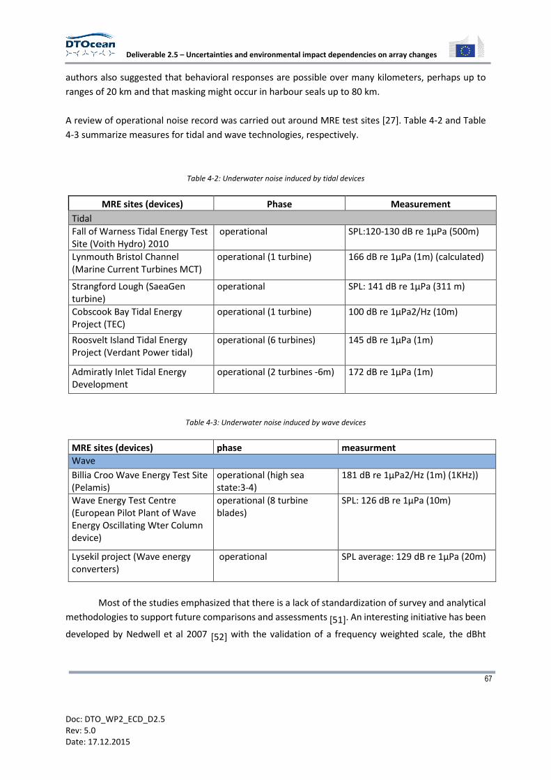
Deliverable 2.5 – Uncertainties and environmental impact dependencies on array changes
67
Doc: DTO_WP2_ECD_D2.5
Rev: 5.0
Date: 17.12.2015
authors also suggested that behavioral responses are possible over many kilometers, perhaps up to
ranges of 20 km and that masking might occur in harbour seals up to 80 km.
A review of operational noise record was carried out around MRE test sites [27]. Table 4-2 and Table
4-3 summarize measures for tidal and wave technologies, respectively.
Table 4-2: Underwater noise induced by tidal devices
MRE sites (devices) Phase Measurement
Tidal
Fall of Warness Tidal Energy Test
Site (Voith Hydro) 2010
operational SPL:120-130 dB re 1µPa (500m)
Lynmouth Bristol Channel
(Marine Current Turbines MCT)
operational (1 turbine) 166 dB re 1µPa (1m) (calculated)
Strangford Lough (SaeaGen
turbine)
operational SPL: 141 dB re 1µPa (311 m)
Cobscook Bay Tidal Energy
Project (TEC)
operational (1 turbine) 100 dB re 1µPa2/Hz (10m)
Roosvelt Island Tidal Energy
Project (Verdant Power tidal)
operational (6 turbines) 145 dB re 1µPa (1m)
Admiratly Inlet Tidal Energy
Development
operational (2 turbines -6m) 172 dB re 1µPa (1m)
Table 4-3: Underwater noise induced by wave devices
MRE sites (devices) phase measurment
Wave
Billia Croo Wave Energy Test Site
(Pelamis)
operational (high sea
state:3-4)
181 dB re 1µPa2/Hz (1m) (1KHz))
Wave Energy Test Centre
(European Pilot Plant of Wave
Energy Oscillating Wter Column
device)
operational (8 turbine
blades)
SPL: 126 dB re 1µPa (10m)
Lysekil project (Wave energy
converters)
operational SPL average: 129 dB re 1µPa (20m)
Most of the studies emphasized that there is a lack of standardization of survey and analytical
methodologies to support future comparisons and assessments [51]. An interesting initiative has been
developed by Nedwell et al 2007 [52] with the validation of a frequency weighted scale, the dBht

Deliverable 2.5 – Uncertainties and environmental impact dependencies on array changes
68
Doc: DTO_WP2_ECD_D2.5
Rev: 5.0
Date: 17.12.2015
(Species), as a metric for the assessment of the behavioral and audiological effects on underwater
animals of man-made underwater noise.
The dBht (Species) metric has been developed to quantify the potential impact on the marine
species behaviours [52] . As any given sound will be perceived differently by different species (since
they have different hearing abilities) the species name must be appended when specifying a level.
For instance, the same construction event might have a level of 70 dBht (Salmo salar) for a
salmon, and 110 dBht (Tursiops truncatus) for a bottlenose dolphin.
Table 4-4 below summarizes the assessment criteria when using the dBht (Species) process
[46]:
Table 4-4: Assessment criteria [50] used in this study to assess the potential behavioral impact of underwater noise on
marine species.
Level in dBht(Species) Effect
90 and above Strong avoidance reaction by virtually all individuals.
Above 110 Tolerance limit of sound; unbearably loud.
Above 130 Possibility of traumatic hearing damage from single event.
In addition, a lower level of 75dBht has sometimes been used for analysis as a level of “significant
avoidance”. At this level, about 85% of individual organisms will react to the noise, although the effect
will probably be limited by habituation [46].
Based on the evidence of auditory damage from the public domain, studies [53] propose a set of
auditory injury criteria based on peak pressure levels and M-weighted Sound Exposure Levels (Table
4-5) (dB re. 1 μPa2/s (M).
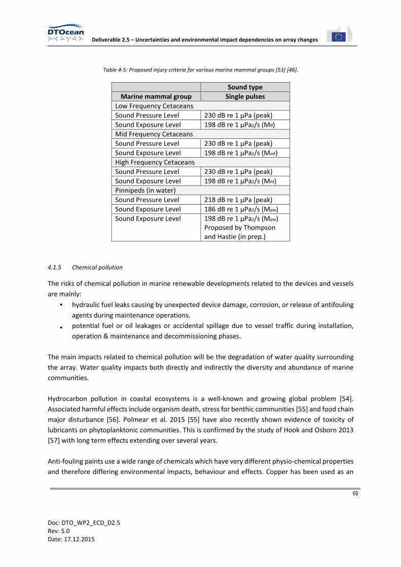
Deliverable 2.5 – Uncertainties and environmental impact dependencies on array changes
69
Doc: DTO_WP2_ECD_D2.5
Rev: 5.0
Date: 17.12.2015
Table 4-5: Proposed injury criteria for various marine mammal groups [53] [46].
Sound type
Marine mammal group Single pulses
Low Frequency Cetaceans
Sound Pressure Level 230 dB re 1 μPa (peak)
Sound Exposure Level 198 dB re 1 μPa2/s (Mlf)
Mid Frequency Cetaceans
Sound Pressure Level 230 dB re 1 μPa (peak)
Sound Exposure Level 198 dB re 1 μPa2/s (Mmf)
High Frequency Cetaceans
Sound Pressure Level 230 dB re 1 μPa (peak)
Sound Exposure Level 198 dB re 1 μPa2/s (Mhf)
Pinnipeds (in water)
Sound Pressure Level 218 dB re 1 μPa (peak)
Sound Exposure Level 186 dB re 1 μPa2/s (Mpw)
Sound Exposure Level 198 dB re 1 μPa2/s (Mpw)
Proposed by Thompson
and Hastie (in prep.)
4.1.5 Chemical pollution
The risks of chemical pollution in marine renewable developments related to the devices and vessels
are mainly:
• hydraulic fuel leaks causing by unexpected device damage, corrosion, or release of antifouling
agents during maintenance operations.
• potential fuel or oil leakages or accidental spillage due to vessel traffic during installation,
operation & maintenance and decommissioning phases.
The main impacts related to chemical pollution will be the degradation of water quality surrounding
the array. Water quality impacts both directly and indirectly the diversity and abundance of marine
communities.
Hydrocarbon pollution in coastal ecosystems is a well-known and growing global problem [54].
Associated harmful effects include organism death, stress for benthic communities [55] and food chain
major disturbance [56]. Polmear et al. 2015 [55] have also recently shown evidence of toxicity of
lubricants on phytoplanktonic communities. This is confirmed by the study of Hook and Osborn 2013
[57] with long term effects extending over several years.
Anti-fouling paints use a wide range of chemicals which have very different physio-chemical properties
and therefore differing environmental impacts, behaviour and effects. Copper has been used as an
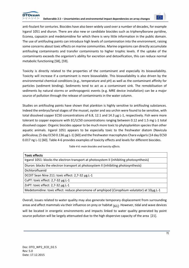
Deliverable 2.5 – Uncertainties and environmental impact dependencies on array changes
70
Doc: DTO_WP2_ECD_D2.5
Rev: 5.0
Date: 17.12.2015
anti-foulant for centuries. Biocides have also been widely used over a number of decades, for example
Irgarol 1051 and diuron. There are also new or candidate biocides such as triphenylborane pyridine,
Econea, capsaicin and medetomidine for which there is very little information in the public domain.
The use of antifouling paints can introduce high levels of contamination into the environment, raising
some concerns about toxic effects on marine communities. Marine organisms can directly accumulate
antifouling contaminants and transfer contaminants to higher trophic levels. If the uptake of the
contaminants exceeds the organism’s ability for excretion and detoxification, this can reduce normal
metabolic functioning [58], [59].
Toxicity is directly related to the properties of the contaminant and especially its bioavailability.
Toxicity will increase if a contaminant is more bioavailable. This bioavailability is also driven by the
environmental chemical conditions (e.g., temperature and pH) as well as the contaminant affinity for
particles (sediment binding). Sediments tend to act as a contaminant sink. The remobilisation of
sediments by natural storms or anthropogenic events (e.g. MRE device installation) can be a major
source of pollution through the release of contaminants in the water column.
Studies on antifouling paints have shown that plankton is highly sensitive to antifouling substances.
Indeed the embryo/larval stages of the mussel, oyster and sea urchin were found to be sensitive, with
total dissolved copper EC50 concentrations of 6.8, 12.1 and 14.3 µg L-1, respectively. Fish were more
tolerant to copper exposure with EC/LC50 concentrations ranging between 0.12 and 1.5 mg L-1 total
dissolved copper. Organic biocides appear to be much more toxic to phytoplankton species than other
aquatic animals. Irgarol 1051 appears to be especially toxic to the freshwater diatom (Navicula
pelliculosa; (5 day EC50 0.136 µg L-1) [60] and the freshwater macrophytes Chara vulgaris (14 day EC50
0.017 ng L-1) [60]. Table 4-6 provides examples of toxicity effects and levels for different biocides.
Table 4-6: main biocides and toxicity effects.
Toxic effects
Irgarol 1051: blocks the electron transport at photosystem II (inhibiting photosynthesis)
Diuron: blocks the electron transport at photosystem II (inhibiting photosynthesis)
Dichlorofluanid
DCOIT Sean Nine 211: toxic effect: 2,7-32 µg.L-1
CuPT: toxic effect: 2,7-32 µg.L-1
ZnPT: toxic effect: 2,7-32 µg.L-1
Medetomidine: toxic effect: reduce pheromone of amphipod (Corophium volutator) at 10µg.L-1
Overall, issues related to water quality may also generate temporary displacement from surrounding
areas and affect mammals via their influence on prey or habitat [61]. However, tidal and wave devices
will be located in energetic environments and impacts linked to water quality generated by point
source pollution will be largely attenuated due to the high dispersive capacity of the area [21].
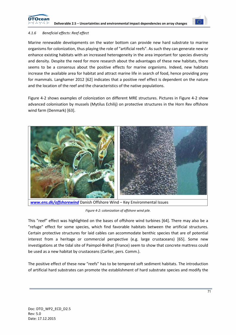
Deliverable 2.5 – Uncertainties and environmental impact dependencies on array changes
71
Doc: DTO_WP2_ECD_D2.5
Rev: 5.0
Date: 17.12.2015
4.1.6 Beneficial effects: Reef effect
Marine renewable developments on the water bottom can provide new hard substrate to marine
organisms for colonization, thus playing the role of "artificial reefs". As such they can generate new or
enhance existing habitats with an increased heterogeneity in the area important for species diversity
and density. Despite the need for more research about the advantages of these new habitats, there
seems to be a consensus about the positive effects for marine organisms. Indeed, new habitats
increase the available area for habitat and attract marine life in search of food, hence providing prey
for mammals. Langhamer 2012 [62] indicates that a positive reef effect is dependent on the nature
and the location of the reef and the characteristics of the native populations.
Figure 4-2 shows examples of colonization on different MRE structures. Pictures in Figure 4-2 show
advanced colonisation by mussels (Mytilus Echilij) on protective structures in the Horn Rev offshore
wind farm (Denmark) [63].
www.ens.dk/offshorewind Danish Offshore Wind – Key Environmental Issues
Figure 4-2: colonization of offshore wind pile.
This "reef" effect was highlighted on the bases of offshore wind turbines [64]. There may also be a
"refuge" effect for some species, which find favorable habitats between the artificial structures.
Certain protective structures for laid cables can accommodate benthic species that are of potential
interest from a heritage or commercial perspective (e.g. large crustaceans) [65]. Some new
investigations at the tidal site of Paimpol-Bréhat (France) seem to show that concrete mattress could
be used as a new habitat by crustaceans (Carlier, pers. Comm.).
The positive effect of these new “reefs” has to be tempered soft sediment habitats. The introduction
of artificial hard substrates can promote the establishment of hard substrate species and modify the
Deliverable 2.5 – Uncertainties and environmental impact dependencies on array changes
72
Doc: DTO_WP2_ECD_D2.5
Rev: 5.0
Date: 17.12.2015
initial habitat. These new hard substrates can also promote introduced species (including invasive
species), and accelerate their geographic expansion by playing the role of "bridgehead" [66].
4.1.7 Beneficial effects: Reserve effect
The physical presence of MRE developments will affect the use of areas with restricted access to these
areas. Despite leading to discussions and conflict regarding recreational and commercial activities,
these new 'preserved' areas will act as small marine protected areas (MPAs). Inger et al. (2009) [36]
highlight the fact that MPAs, where all fisheries and other forms of extraction are excluded, can be
used as a fisheries management, conservation and ecological restoration tool.
As well as protecting and enhancing fish stocks, the implementation of such MPAs will also enrich
benthic biota, by lifting the pressure from towed bottom fishing gear [67], which has chronic effects
on seabed communities and is likely to affect ecosystem functioning [43].
Impact will vary depending on the restriction measures in place but. fishing restriction creates a marine
protected area that will have positive impacts on biodiversity, and juvenile’s and reproductive adult’s
protection [68]. These effects have already been observed in offshore windfarms [69]. However, it is
important to remember that the location, and hence the habitat protected by this potential reserve
effect, could also be valuable in terms of conservation, restoration for surrounding fishery [36].
4.1.8 Resting place
Emerged structure can be used as resting platforms mainly for birds and pinnipeds depending on
their accessibility. This positive impact is of course only considered during the operation phase of the
project. In open sea where resting places could be rare, these structures will create new habitats.
Species such as gulls, terns and cormorants show no avoidance response to emerged MRE structures
and may instead be attracted to theses installations through prey aggregation and their use as
resting/foraging platforms [65]. This latter study indicates that effects would be species-specific.
The positive impact is however only valuable if it is not dangerous for the animals to stand on the
structures.
4.2 General recommendations
4.2.1 Energy modification
• Design devices and arrays in order to minimize the water velocity effect and the bottom
substrate effect
• Foster design of devices based on floating platforms (substrate and sediment transport are
minimized) [18]
• Minimize power dissipation

Deliverable 2.5 – Uncertainties and environmental impact dependencies on array changes
73
Doc: DTO_WP2_ECD_D2.5
Rev: 5.0
Date: 17.12.2015
4.2.2 Collision risk
• Have a good knowledge of the sensitive species (mostly marine mammals) in the project area
• Choose device composition and material that reduce the risk of collision and entanglement,
for example: [18], [28]
- By increasing the detectability of the device by animals (use specific color).
• Locate device in a specific area (bathymetry, etc.)
• Choose appropriate device for the area and species in this area (reducing vertical traps)
4.2.3 Turbidity
• Try to choose a low impact design and operation of device regarding sediment disturbance
• Adjust the rotation velocity of the device (tidal)
4.2.4 Underwater noise
• Have a good knowledge of the sensitive species in the area
• Use of sound insulation around the device [18]
• Use of acoustic mitigation to exclude animals from the area
• Have a good knowledge of sensitive area and locate the project away from the sensitive area
• Limit the size of the project
4.2.5 Chemical pollution
• Design of the device: minimize the volume of lubricants and chemical fluid
• Use of new less toxic antifouling substances
4.2.6 Reef effect
• Choose a design that will increase their colonization potential
• Reduce antifouling protection
• Locate device in water deeper than 20 meters [18]

Deliverable 2.5 – Uncertainties and environmental impact dependencies on array changes
74
Doc: DTO_WP2_ECD_D2.5
Rev: 5.0
Date: 17.12.2015
4.2.7 Reserve effect
• Adapt activity restriction measures to the project and to the habitats and species found in the
area.
4.2.8 Resting place
• Secure safe part of device that could be used as resting place by birds or pinnipeds.
• Minimize horizontal surfaces of devices to limit the resting place for marine mammals and
birds if these parts of device are dangerous.
4.3 EIAM environmental process
The whole EIAM is based on several scoring principles detailed in Deliverable 7.2. Briefly, the use of
the environmental functions allows the EIAM to generate numerical values that will be converted in to
environmental scores (Environmental impact score) (Figure 4-3). The conversion from the function
scores to the environmental scores is made through calibration matrices. Each function is associated
with one calibration matrix (or several depending of the complexity of the function) in order to qualify
the pressure score. Calibration matrices are based on literature data.
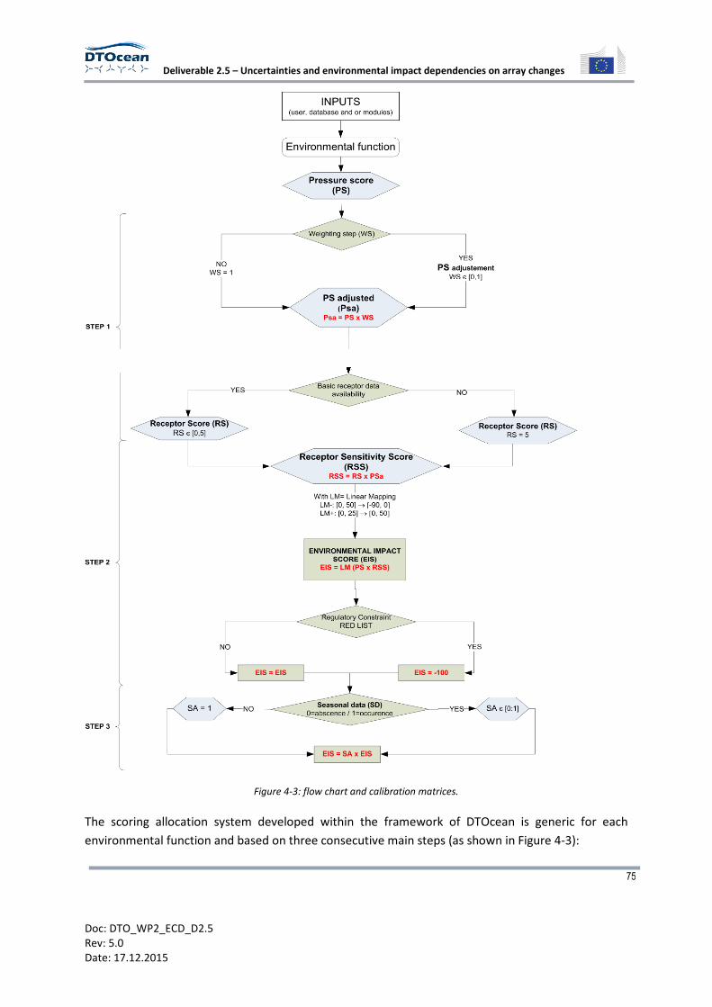
Deliverable 2.5 – Uncertainties and environmental impact dependencies on array changes
75
Doc: DTO_WP2_ECD_D2.5
Rev: 5.0
Date: 17.12.2015
Figure 4-3: flow chart and calibration matrices.
The scoring allocation system developed within the framework of DTOcean is generic for each
environmental function and based on three consecutive main steps (as shown in Figure 4-3):
Deliverable 2.5 – Uncertainties and environmental impact dependencies on array changes
76
Doc: DTO_WP2_ECD_D2.5
Rev: 5.0
Date: 17.12.2015
• STEP 1: qualification and quantification of the 'pressure' generated by the stressors.
• STEP 2: basic qualification of the occurrence (or absence) of receptors potentially affected by
the stressors. If the chosen receptors in the basic receptor database are also in the red list, the
Receptor sensitivity score doesn’t use the standard qualification of the score, but takes the
maximum score 100.
• STEP 3: qualification refinement of receptors e.g. definition of slot of occurrence
during the year where receptors are sensitive (ie nesting seasons for birds, breeding
seasons for mammals...).
4.4 EIAM environmental functions associated with hydrodynamics
All the parameters involved in the environmental processes are presented in this section. Stressors
create the pressure and receptors are the sensitive animal and vegetal species impacted by the
stressors. The environmental function uses inputs to produce a result. As shown in Figure 4-3, a
weighting factor can also occur in the first step of the evaluation process to better qualify the pressure.
Some definitions:
• Stressors: Stressors are the physical anthropogenic elements that generate the 'footprint'
pressure.
• Receptors: Receptors are all the biological components (animal and vegetal species, habitats)
potentially impacted by the stressors.
• Weighting step: The weighting score ranges between 0 and 1. If there is no data for the
constraints, the precautionary principle lead to the worst weighting case: 1.
• Inputs: To quantify the pressure and the impact, some parameters or inputs are required. They
are provided by the DTOcean database, the other modules or the user.
4.4.1 Environmental function: energy modification
Objective
The aim of this function is to assess the impact of current and wave energy modification due to
arrays on biological receptors.
Stressors
In the Array Hydrodynamic issue the energy modification is induced by the extraction of the current
and wave energy by the devices. Incoming and outgoing energy from arrays is used to calculate the
percentage of energy extracted by arrays.
Receptors
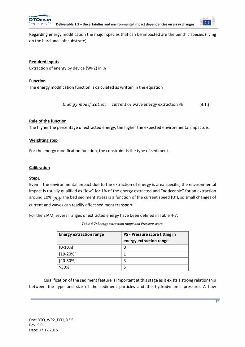
Deliverable 2.5 – Uncertainties and environmental impact dependencies on array changes
77
Doc: DTO_WP2_ECD_D2.5
Rev: 5.0
Date: 17.12.2015
Regarding energy modification the major species that can be impacted are the benthic species (living
on the hard and soft substrate).
Required inputs
Extraction of energy by device (WP2) in %
Function
The energy modification function is calculated as written in the equation
234-0�516!6789653 � currentorwaveenergyextraction% (4.1.)
Rule of the function
The higher the percentage of extracted energy, the higher the expected environmental impacts is.
Weighting step
For the energy modification function, the constraint is the type of sediment.
Calibration
Step1
Even if the environmental impact due to the extraction of energy is area specific, the environmental
impact is usually qualified as “low” for 1% of the energy extracted and “noticeable” for an extraction
around 10% [70]. The bed sediment stress is a function of the current speed (U2), so small changes of
current and waves can readily affect sediment transport.
For the EIAM, several ranges of extracted energy have been defined in Table 4-7:
Table 4-7: Energy extraction range and Pressure score.
Energy extraction range PS - Pressure score fitting in
energy extraction range
[0-10%[ 0
[10-20%[ 1
[20-30%] 3
>30% 5
Qualification of the sediment feature is important at this stage as it exists a strong relationship
between the type and size of the sediment particles and the hydrodynamic pressure. A flow
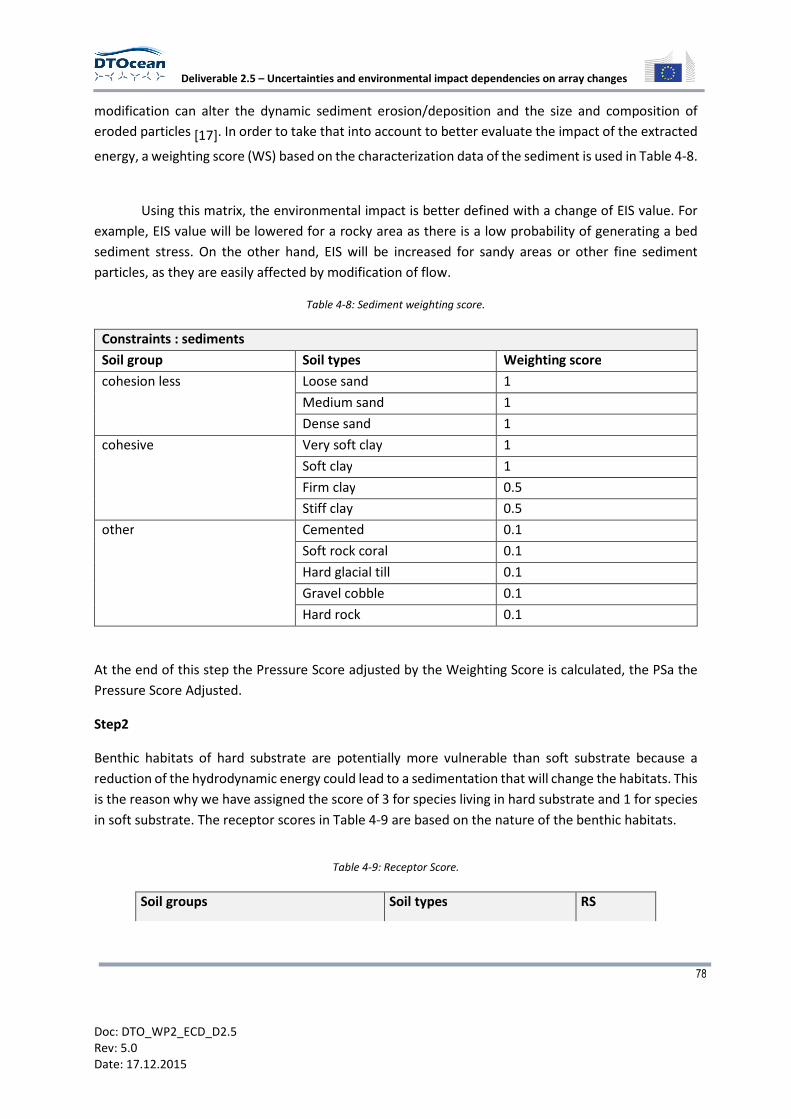
Deliverable 2.5 – Uncertainties and environmental impact dependencies on array changes
78
Doc: DTO_WP2_ECD_D2.5
Rev: 5.0
Date: 17.12.2015
modification can alter the dynamic sediment erosion/deposition and the size and composition of
eroded particles [17]. In order to take that into account to better evaluate the impact of the extracted
energy, a weighting score (WS) based on the characterization data of the sediment is used in Table 4-8.
Using this matrix, the environmental impact is better defined with a change of EIS value. For
example, EIS value will be lowered for a rocky area as there is a low probability of generating a bed
sediment stress. On the other hand, EIS will be increased for sandy areas or other fine sediment
particles, as they are easily affected by modification of flow.
Table 4-8: Sediment weighting score.
Constraints : sediments
Soil group Soil types Weighting score
cohesion less Loose sand 1
Medium sand 1
Dense sand 1
cohesive Very soft clay 1
Soft clay 1
Firm clay 0.5
Stiff clay 0.5
other Cemented 0.1
Soft rock coral 0.1
Hard glacial till 0.1
Gravel cobble 0.1
Hard rock 0.1
At the end of this step the Pressure Score adjusted by the Weighting Score is calculated, the PSa the
Pressure Score Adjusted.
Step2
Benthic habitats of hard substrate are potentially more vulnerable than soft substrate because a
reduction of the hydrodynamic energy could lead to a sedimentation that will change the habitats. This
is the reason why we have assigned the score of 3 for species living in hard substrate and 1 for species
in soft substrate. The receptor scores in Table 4-9 are based on the nature of the benthic habitats.
Table 4-9: Receptor Score.
Soil groups Soil types RS
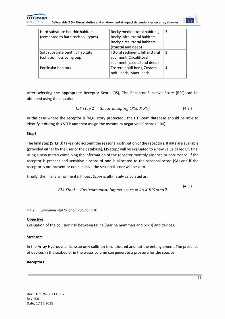
Deliverable 2.5 – Uncertainties and environmental impact dependencies on array changes
79
Doc: DTO_WP2_ECD_D2.5
Rev: 5.0
Date: 17.12.2015
Hard substrate benthic habitats
(cemented to hard rock soil types)
Rocky mediolittoral habitats,
Rocky infralittoral habitats,
Rocky circalittoral habitats
(coastal and deep)
3
Soft substrate benthic habitats
(cohesion less soil group)
littoral sediment, Infralittoral
sediment, Circalittoral
sediment (coastal and deep)
1
Particular habitats Zostera noltii beds, Zostera
noltii beds, Maerl beds
4
After selecting the appropriate Receptor Score (RS), The Receptor Sensitive Score (RSS) can be
obtained using the equation
2I�J94K2 � M6348-88K630�N�8OP�� (4.2.)
In the case where the receptor is 'regulatory protected', the DTOcean database should be able to
identify it during this STEP and then assign the maximum negative EIS score (-100).
Step3
The final step (STEP 3) takes into account the seasonal distribution of the receptors. If data are available
(provided either by the user or the database), EIS step2 will be evaluated to a new value called EIS final
using a new matrix containing the information of the receptor monthly absence or occurrence. If the
receptor is present and sensitive a score of one is allocated to the seasonal score (SA) and if the
receptor is not present or not sensitive the seasonal score will be zero.
Finally, the final Environmental Impact Score is ultimately calculated as:
2I�!638M � 23Q6-534398M6K879J75-4 � �RO2I�J94K2
(4.3.)
4.4.2 Environmental function: collision risk
Objective
Evaluation of the collision risk between fauna (marine mammals and birds) and devices.
Stressors
In the Array Hydrodynamic issue only collision is considered and not the entanglement. The presence
of devices in the seabed or in the water column can generate a pressure for the species.
Receptors

Deliverable 2.5 – Uncertainties and environmental impact dependencies on array changes
80
Doc: DTO_WP2_ECD_D2.5
Rev: 5.0
Date: 17.12.2015
Regarding the collision risks between animals and devices, the major species that can be impacted are
mainly marine mammals and birds. For both species the position of the devices in the water column
has to be taken into account.
Required inputs
• cross sectional area of the farm
• Number of devices
• Volume of the device
Function
Work in progress (4.1.)
Rule of the function
0 ≤ ratio ≤ 1
0 = green, increase = goes towards red
The placement of devices and depth are important to determine the collision risk.
Weighting step
For the collision risk function, the constraints are the position and the location of the devices.
Calibration
Step1
To qualify score and calibration, some data found in the literature review have been used. A feedback
of this collection is proposed in this chapter. To quantify the collision risk “Pressure Score” PS an
arbitrary method was used. After obtaining the result of the function, the data is classified at one of 3
levels.
Above 25% of space occupied by devices, the collision risk is estimated as high. A weight is given for
each category dependent on the risk of collision for a specie in Table 4-10.
Table 4-10: Calibration risk range and Pressure Score.
Collision risks range PS - Pressure score fitting in
collision risk range
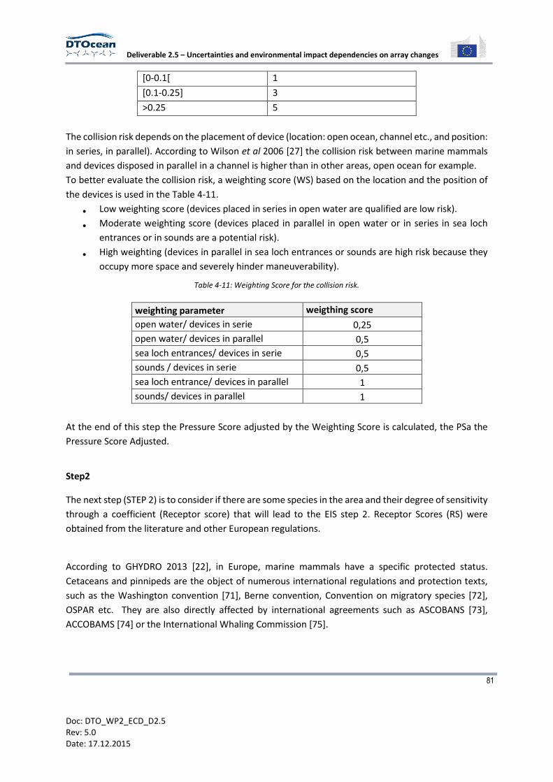
Deliverable 2.5 – Uncertainties and environmental impact dependencies on array changes
81
Doc: DTO_WP2_ECD_D2.5
Rev: 5.0
Date: 17.12.2015
[0-0.1[ 1
[0.1-0.25] 3
>0.25 5
The collision risk depends on the placement of device (location: open ocean, channel etc., and position:
in series, in parallel). According to Wilson et al 2006 [27] the collision risk between marine mammals
and devices disposed in parallel in a channel is higher than in other areas, open ocean for example.
To better evaluate the collision risk, a weighting score (WS) based on the location and the position of
the devices is used in the Table 4-11.
• Low weighting score (devices placed in series in open water are qualified are low risk).
• Moderate weighting score (devices placed in parallel in open water or in series in sea loch
entrances or in sounds are a potential risk).
• High weighting (devices in parallel in sea loch entrances or sounds are high risk because they
occupy more space and severely hinder maneuverability).
Table 4-11: Weighting Score for the collision risk.
weighting parameter weigthing score
open water/ devices in serie 0,25
open water/ devices in parallel 0,5
sea loch entrances/ devices in serie 0,5
sounds / devices in serie 0,5
sea loch entrance/ devices in parallel 1
sounds/ devices in parallel 1
At the end of this step the Pressure Score adjusted by the Weighting Score is calculated, the PSa the
Pressure Score Adjusted.
Step2
The next step (STEP 2) is to consider if there are some species in the area and their degree of sensitivity
through a coefficient (Receptor score) that will lead to the EIS step 2. Receptor Scores (RS) were
obtained from the literature and other European regulations.
According to GHYDRO 2013 [22], in Europe, marine mammals have a specific protected status.
Cetaceans and pinnipeds are the object of numerous international regulations and protection texts,
such as the Washington convention [71], Berne convention, Convention on migratory species [72],
OSPAR etc. They are also directly affected by international agreements such as ASCOBANS [73],
ACCOBAMS [74] or the International Whaling Commission [75].
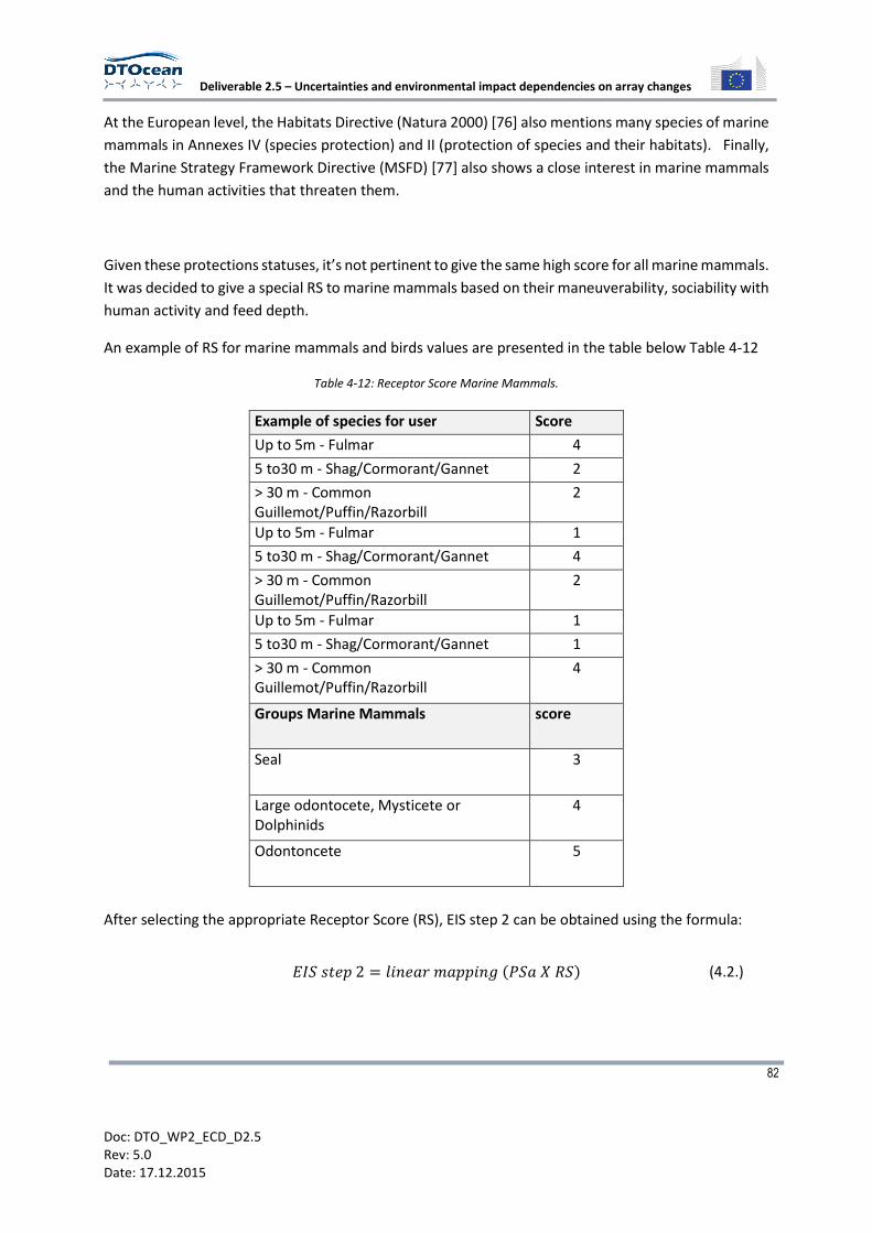
Deliverable 2.5 – Uncertainties and environmental impact dependencies on array changes
82
Doc: DTO_WP2_ECD_D2.5
Rev: 5.0
Date: 17.12.2015
At the European level, the Habitats Directive (Natura 2000) [76] also mentions many species of marine
mammals in Annexes IV (species protection) and II (protection of species and their habitats). Finally,
the Marine Strategy Framework Directive (MSFD) [77] also shows a close interest in marine mammals
and the human activities that threaten them.
Given these protections statuses, it’s not pertinent to give the same high score for all marine mammals.
It was decided to give a special RS to marine mammals based on their maneuverability, sociability with
human activity and feed depth.
An example of RS for marine mammals and birds values are presented in the table below Table 4-12
Table 4-12: Receptor Score Marine Mammals.
Example of species for user Score
Up to 5m - Fulmar 4
5 to30 m - Shag/Cormorant/Gannet 2
> 30 m - Common
Guillemot/Puffin/Razorbill
2
Up to 5m - Fulmar 1
5 to30 m - Shag/Cormorant/Gannet 4
> 30 m - Common
Guillemot/Puffin/Razorbill
2
Up to 5m - Fulmar 1
5 to30 m - Shag/Cormorant/Gannet 1
> 30 m - Common
Guillemot/Puffin/Razorbill
4
Groups Marine Mammals score
Seal 3
Large odontocete, Mysticete or
Dolphinids
4
Odontoncete 5
After selecting the appropriate Receptor Score (RS), EIS step 2 can be obtained using the formula:
2I�J94K2 � M6348-8KK630�N�8OP�� (4.2.)
Deliverable 2.5 – Uncertainties and environmental impact dependencies on array changes
83
Doc: DTO_WP2_ECD_D2.5
Rev: 5.0
Date: 17.12.2015
In the case where the receptor is 'regulatory protected', the DTOcean database should be able
to identify it during this STEP and then assign the maximum negative EIS score (-100).
Step 3
The final step (STEP 3) takes into account the seasonal distribution of the receptors. If data are available
(provided either by the user or the database), EIS step2 will be evaluated to a new value called EIS final
using a new matrix containing the information of the receptor monthly absence or occurrence. If there
is data the seasonal score (SA) is allocated with a score of one and if there is no data the seasonal score
is allocated of a score of zero.
The final Environmental Impact Score is ultimately calculated as follow
2I�!638M � 23Q6-534398M6K879J75-4 � �RO2I�J94K2 (4.3.)
4.4.3 Environmental function: Turbidity
Objective
Evaluation of the impact of the turbidity modification intensity in the water column due to arrays.
Stressors
In the Array Hydrodynamic issue is considered a stressor for the turbidity function, the turbidity
created during the operational phase of the devices.
Receptors
The turbidity created during the installation phase is a physical pressure that can affect benthos and
the benthic habitats of cohesion less soils, cohesive soils or cemented and rocky soils, but also fishes,
marine mammals and sea birds.
Inputs
• initial turbidity
• turbidity measured during the operational phase
Function
Turbiditymodification� Comparisonbetweeninitialturbidityandturbidity
(4.4.)

Deliverable 2.5 – Uncertainties and environmental impact dependencies on array changes
84
Doc: DTO_WP2_ECD_D2.5
Rev: 5.0
Date: 17.12.2015
measuredduringtheoperationalphase
Rule
The rule of this function is to estimate the difference in turbidity between the initial state and the
turbidity measured during the operational phase. If the turbidity measured during the operational
phase is higher than the initial state, the pressure is considered as major in application of the
precautionary principle.
Weighting step
There is no particular constraint for the turbidity function. According to the precautionary principle,
the weighting score is calibrated for the worst pressure case with a score of 1.
Calibration
Step 1
The difficulty to quantify this environmental impact is related to the high variability of turbidity in
coastal waters [78]. Typical concentrations range from few mg/l to hundreds mg/l during storm events
or near estuarine areas. To quantify the turbidity risk we utilize a binary method which consists of
comparing the initial turbidity and turbidity during the installation phase in the Table 4-13.
Table 4-13: calibration pressure score for the turbidity risk.
Result of the function Pressure Score - PS
turbidity stressor < initial turbidity 0
turbidity stressor ≥ initial turbidity 5
Step 2
The hard substrate benthic habitats are potentiality more vulnerable by an increase of turbidity than
soft substrate habitats because of the macroalgea. These macroalgea are indeed among the key
species of the benthic habitats of hard substrate and the diminution of light induced by the increase
of the turbidity directly affects them. That is the reason why we have assigned the score of 3 for
species living in hard substrata and 1 for species in soft substrata. Marine mammals and birds can also
be impacted by the increase of the turbidity but the lack of data and the low potential risk has led to a
score of 1in the Table 4-14.

Deliverable 2.5 – Uncertainties and environmental impact dependencies on array changes
85
Doc: DTO_WP2_ECD_D2.5
Rev: 5.0
Date: 17.12.2015
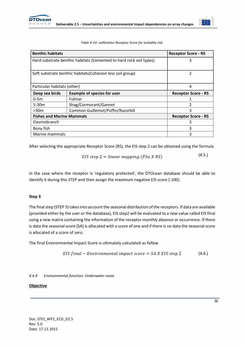
Deliverable 2.5 – Uncertainties and environmental impact dependencies on array changes
86
Doc: DTO_WP2_ECD_D2.5
Rev: 5.0
Date: 17.12.2015
Table 4-14: calibration Receptor Score for turbidity risk.
Benthic habitats Receptor Score - RS
Hard substrate benthic habitats (Cemented to hard rock soil types) 3
Soft substrate benthic habitats(Cohesion less soil group) 2
Particular habitats (other) 4
Deep sea birds Example of species for user Receptor Score - RS
0-5m Fulmar 1
5-30m Shag/Cormorant/Gannet 2
>30m Common Guillemot/Puffin/Razorbill 3
Fishes and Marine Mammals Receptor Score - RS
Elasmobranch 3
Bony fish 3
Marine mammals 3
After selecting the appropriate Receptor Score (RS), the EIS step 2 can be obtained using the formula
2I�J94K2 � M6348-8KK630�N�8OP�� (4.5.)
In the case where the receptor is 'regulatory protected', the DTOcean database should be able to
identify it during this STEP and then assign the maximum negative EIS score (-100).
Step 3
The final step (STEP 3) takes into account the seasonal distribution of the receptors. If data are available
(provided either by the user or the database), EIS step2 will be evaluated to a new value called EIS final
using a new matrix containing the information of the receptor monthly absence or occurrence. If there
is data the seasonal score (SA) is allocated with a score of one and if there is no data the seasonal score
is allocated of a score of zero.
The final Environmental Impact Score is ultimately calculated as follow
2I�!638M � 23Q6-534398M6K879J75-4 � �RO2I�J94K2 (4.6.)
4.4.4 Environmental function: Underwater noise
Objective
Deliverable 2.5 – Uncertainties and environmental impact dependencies on array changes
87
Doc: DTO_WP2_ECD_D2.5
Rev: 5.0
Date: 17.12.2015
The goal of this function is to evaluate the impact of underwater noise produced by the devices
during the operational phase.
Stressors
The noise created during the operational phase of the devices.
Receptors
Underwater noise produced by devices is a physical pressure that can affect marine mammals and
fishes.
Inputs
• Initial underwater noise (=background noise).
• Noise produced by the individual devices [unit: dB re 1µPa (1m)].
Function’s formula
The 'underwater noise' function consists of a comparison between the initial underwater noise and
the underwater noise level produced by the device.
.314-]894-356J4� 75K8-6J535!9^4_314-]894-356J45!9^414Q674J]69^
9^4636698M_314-]894-356J4639^48-48
(4.7.)
Rule
The rule of this function is to estimate the difference between the initial noise and the noise induced
by the devices during the operational phase. If the noise measured during the operational phase is
higher than the initial state, the pressure is considered as major in application of the precautionary
principle.
Weighting step
There is no particular constraint for the underwater noise function. According to the precautionary
principle, the weighting score is calibrated for the worst pressure case with a score of 1.
Calibration
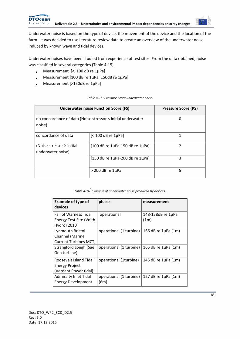
Deliverable 2.5 – Uncertainties and environmental impact dependencies on array changes
88
Doc: DTO_WP2_ECD_D2.5
Rev: 5.0
Date: 17.12.2015
Underwater noise is based on the type of device, the movement of the device and the location of the
farm. It was decided to use literature review data to create an overview of the underwater noise
induced by known wave and tidal devices.
Underwater noises have been studied from experience of test sites. From the data obtained, noise
was classified in several categories (Table 4-15).
• Measurement [<; 100 dB re 1µPa]
• Measurement [100 dB re 1µPa; 150dB re 1µPa]
• Measurement [>150dB re 1µPa]
Table 4-15: Pressure Score underwater noise.
Underwater noise Function Score (FS) Pressure Score (PS)
no concordance of data (Noise stressor < initial underwater
noise)
0
concordance of data
(Noise stressor ≥ initial
underwater noise)
[< 100 dB re 1µPa] 1
[100 dB re 1µPa-150 dB re 1µPa] 2
[150 dB re 1µPa-200 dB re 1µPa] 3
> 200 dB re 1µPa 5
Table 4-16:
Example of underwater noise produced by devices.
Example of type of
devices
phase measurement
Fall of Warness Tidal
Energy Test Site (Voith
Hydro) 2010
operational 148-158dB re 1µPa
(1m)
Lynmouth Bristol
Channel (Marine
Current Turbines MCT)
operational (1 turbine) 166 dB re 1µPa (1m)
Strangford Lough (Sae
Gen turbine)
operational (1 turbine) 165 dB re 1µPa (1m)
Roosevelt Island Tidal
Energy Project
(Verdant Power tidal)
operational (1turbine) 145 dB re 1µPa (1m)
Admiralty Inlet Tidal
Energy Development
operational (1 turbine)
(6m)
127 dB re 1µPa (1m)

Deliverable 2.5 – Uncertainties and environmental impact dependencies on array changes
89
Doc: DTO_WP2_ECD_D2.5
Rev: 5.0
Date: 17.12.2015
Wave Energy Test
Centre (European Pilot
Plant of Wave Energy
Oscillating Water
Column device)
operational (1 turbine) 151 dB re 1µPa (1m)
Lysekil project (Wave
energy converters)
operational 158 dB re 1µPa (1m)
Legends: [27]
dB: decibel
SPL: Sound Pressure Level; the level of the RMS sound pressure. SPL is a root mean square (RMS)
quantity and averaging time must be defined.
PTS: Permanent Threshold Shift; auditory damage in the form of permanent hearing sensitivity
reduction
TTS: Temporary Threshold Shift (recoverable auditory fatigue)
Step 2
To discriminate in term of sensibility, Step 2 involves three expected type of effect:
� behavioral modification of species,
� TTS - temporal threshold shift,
� PTS - permanent threshold shift.
Behavior effect is considered as a moderate effect unlike TTS and PTS that are considered as major
effects because of the potential physiological issues they can generate. So receptor scores are based
on the following assignment:
� Behavioral modification: score 3
� TTS: score 5
� PTS: score 5
Values in each level (Behavioral, TTS and PTS) are also species specific. Some examples are given in
Table 4-17.
Table 4-17: Receptor Score for the underwater noise function.
Sensitivity threshold Species Effect RS
< 143 dB re 1µPa Large Odontoncete, odontoncetes,
Delphinids, Mysticetes
behavioural 3
[143-224] dB re 1µPa TTS 5
>224 dB re 1µPa PTS 5
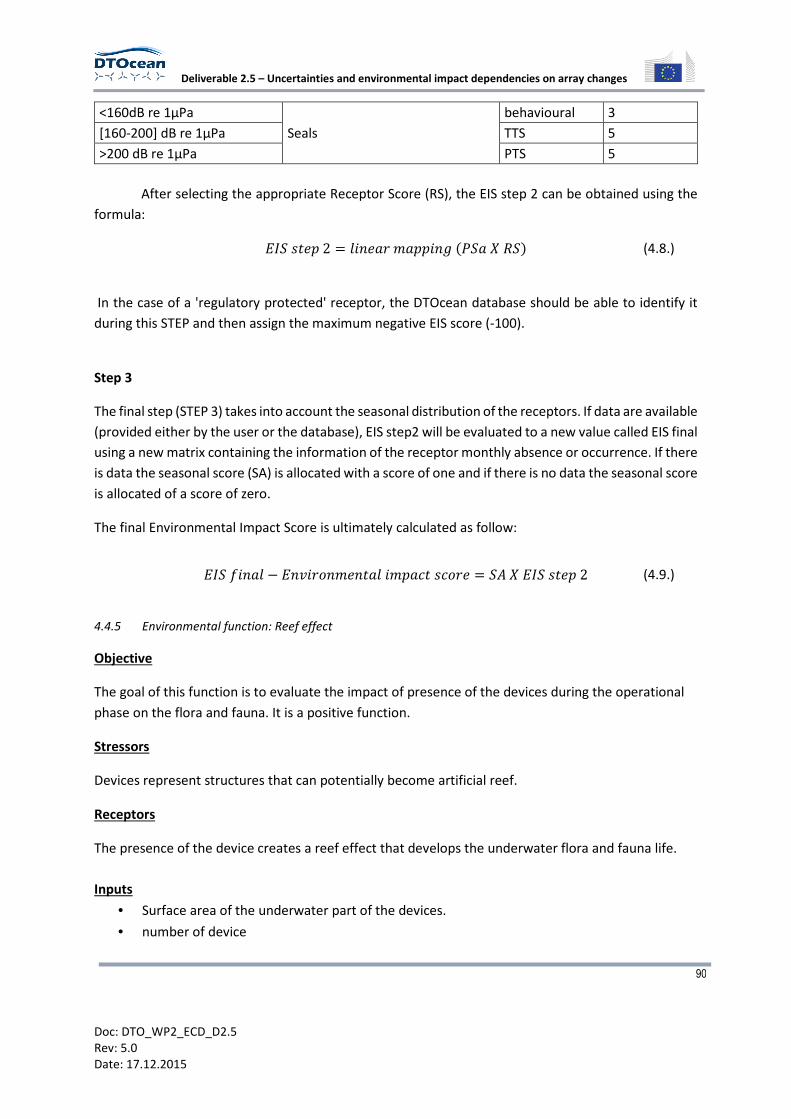
Deliverable 2.5 – Uncertainties and environmental impact dependencies on array changes
90
Doc: DTO_WP2_ECD_D2.5
Rev: 5.0
Date: 17.12.2015
<160dB re 1µPa
Seals
behavioural 3
[160-200] dB re 1µPa TTS 5
>200 dB re 1µPa PTS 5
After selecting the appropriate Receptor Score (RS), the EIS step 2 can be obtained using the
formula:
2I�J94K2 � M6348-8KK630�N�8OP�� (4.8.)
In the case of a 'regulatory protected' receptor, the DTOcean database should be able to identify it
during this STEP and then assign the maximum negative EIS score (-100).
Step 3
The final step (STEP 3) takes into account the seasonal distribution of the receptors. If data are available
(provided either by the user or the database), EIS step2 will be evaluated to a new value called EIS final
using a new matrix containing the information of the receptor monthly absence or occurrence. If there
is data the seasonal score (SA) is allocated with a score of one and if there is no data the seasonal score
is allocated of a score of zero.
The final Environmental Impact Score is ultimately calculated as follow:
2I�!638M � 23Q6-534398M6K879J75-4 � �RO2I�J94K2 (4.9.)
4.4.5 Environmental function: Reef effect
Objective
The goal of this function is to evaluate the impact of presence of the devices during the operational
phase on the flora and fauna. It is a positive function.
Stressors
Devices represent structures that can potentially become artificial reef.
Receptors
The presence of the device creates a reef effect that develops the underwater flora and fauna life.
Inputs
• Surface area of the underwater part of the devices.
• number of device
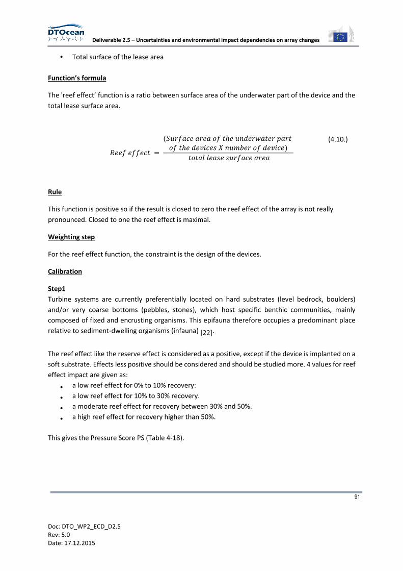
Deliverable 2.5 – Uncertainties and environmental impact dependencies on array changes
91
Doc: DTO_WP2_ECD_D2.5
Rev: 5.0
Date: 17.12.2015
• Total surface of the lease area
Function’s formula
The 'reef effect’ function is a ratio between surface area of the underwater part of the device and the
total lease surface area.
P44!4!!479 �
��_-!8748-485!9^4_314-]894-K8-95!9^414Q674JO3_`4-5!14Q674�
9598MM48J4J_-!8748-48
(4.10.)
Rule
This function is positive so if the result is closed to zero the reef effect of the array is not really
pronounced. Closed to one the reef effect is maximal.
Weighting step
For the reef effect function, the constraint is the design of the devices.
Calibration
Step1
Turbine systems are currently preferentially located on hard substrates (level bedrock, boulders)
and/or very coarse bottoms (pebbles, stones), which host specific benthic communities, mainly
composed of fixed and encrusting organisms. This epifauna therefore occupies a predominant place
relative to sediment-dwelling organisms (infauna) [22].
The reef effect like the reserve effect is considered as a positive, except if the device is implanted on a
soft substrate. Effects less positive should be considered and should be studied more. 4 values for reef
effect impact are given as:
• a low reef effect for 0% to 10% recovery:
• a low reef effect for 10% to 30% recovery.
• a moderate reef effect for recovery between 30% and 50%.
• a high reef effect for recovery higher than 50%.
This gives the Pressure Score PS (Table 4-18).

Deliverable 2.5 – Uncertainties and environmental impact dependencies on array changes
92
Doc: DTO_WP2_ECD_D2.5
Rev: 5.0
Date: 17.12.2015
Table 4-18: Pressure Score of the reef effect.
Reef effect range PS - Pressure score fitting in reef effect range
[0-0.1[ 1
[0.1-0.3[ 2
[0.3-0.5] 3
>0.5 5
According to Langhamer et al 2009 [79], colonization on artificial reef is influenced by the age, texture,
inclination and position in the water column of the reef. Some studies were done on wave devices, and
the assemblage of species depends on the design of the structure. In the words of Langhamer et al
.2009 [79] “Vertical surfaces were more densely colonized than horizontal surfaces […]”.
It is useful to create a Weighting Score (WS) as a function of the design structure (vertical or horizontal)
(Table 4-19).
Table 4-19: Weighting Score for the reef effect.
Types of device Design WS-Weighting Score
Wave horizontal 0.5
Wave vertical 1
Tidal Horizontal 0.5
Tidal vertical 1
At the end of this step the Pressure Score adjusted by the Weighting Score is calculated, the PSa the
Pressure Score Adjusted.
Step 2
It is considered that all benthic habitats can be affected by reef, so the highest score (5) is given
for all organisms. This value is set by default as there is inevitably a reef effect on all structures [56],
[62]. This gives the Receptor Score (Table 4-20).
Table 4-20: Receptor Score for the reef effect.
Receptors RS-Receptor Score
Hard substrate benthic habitats 5
Soft substrate benthic habitats 5
Deliverable 2.5 – Uncertainties and environmental impact dependencies on array changes
93
Doc: DTO_WP2_ECD_D2.5
Rev: 5.0
Date: 17.12.2015
After selecting the appropriate Receptor Score (RS), the EIS step 2 can be obtained using the
formula.
2I�J94K2 � M6348-8KK630�N�8OP�� (4.11.)
Step 3
The final step (STEP 3) takes into account the seasonal distribution of the receptors. If data are available
(provided either by the user or the database), EIS step2 will be evaluated to a new value called EIS final
using a new matrix containing the information of the receptor monthly absence or occurrence. If there
is data the seasonal score (SA) is allocated with a score of one and if there is no data the seasonal score
is allocated a score of zero.
The final Environmental Impact Score is ultimately calculated as follows:
2I�!638M � 23Q6-534398M6K879J75-4 � �RO2I�J94K2 (4.12.)
4.4.6 Environmental function: reserve effect
Objective
Evaluation of the reserve effect of fishery restriction in the tidal and wave arrays. It is a positive
function.
Stressors
The array can have a reserve effect depending on the fishery restrictions.
Receptors
Fishery restriction create a reserve effect that can influence all of the ecosystem.
Inputs
• Fishery restriction surface
• Total lease surface area
Function’s formula
The 'reserve effect’ function is a ratio between the fishery restriction surface and the total lease
surface area.
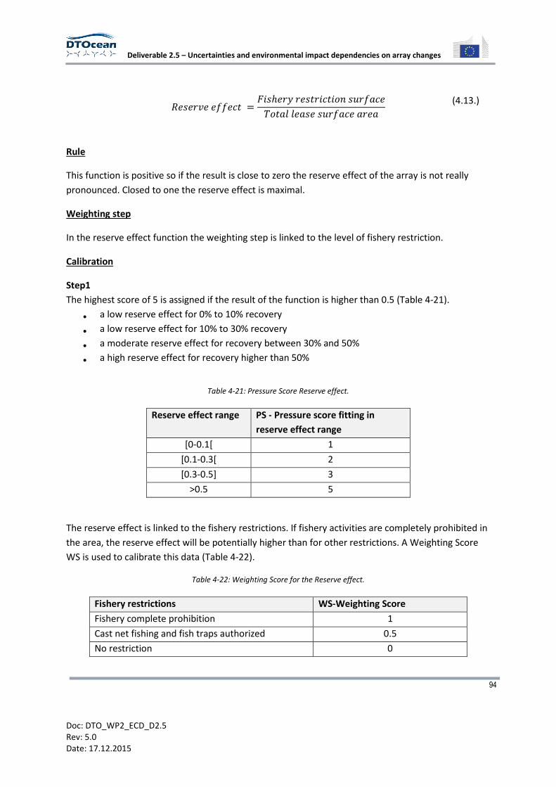
Deliverable 2.5 – Uncertainties and environmental impact dependencies on array changes
94
Doc: DTO_WP2_ECD_D2.5
Rev: 5.0
Date: 17.12.2015
P4J4-Q44!!479 �
,6J^4-�-4J9-679653J_-!874)598MM48J4J_-!8748-48
(4.13.)
Rule
This function is positive so if the result is close to zero the reserve effect of the array is not really
pronounced. Closed to one the reserve effect is maximal.
Weighting step
In the reserve effect function the weighting step is linked to the level of fishery restriction.
Calibration
Step1
The highest score of 5 is assigned if the result of the function is higher than 0.5 (Table 4-21).
• a low reserve effect for 0% to 10% recovery
• a low reserve effect for 10% to 30% recovery
• a moderate reserve effect for recovery between 30% and 50%
• a high reserve effect for recovery higher than 50%
Table 4-21: Pressure Score Reserve effect.
Reserve effect range PS - Pressure score fitting in
reserve effect range
[0-0.1[ 1
[0.1-0.3[ 2
[0.3-0.5] 3
>0.5 5
The reserve effect is linked to the fishery restrictions. If fishery activities are completely prohibited in
the area, the reserve effect will be potentially higher than for other restrictions. A Weighting Score
WS is used to calibrate this data (Table 4-22).
Table 4-22: Weighting Score for the Reserve effect.
Fishery restrictions WS-Weighting Score
Fishery complete prohibition 1
Cast net fishing and fish traps authorized 0.5
No restriction 0

Deliverable 2.5 – Uncertainties and environmental impact dependencies on array changes
95
Doc: DTO_WP2_ECD_D2.5
Rev: 5.0
Date: 17.12.2015
At the end of this step the Pressure Score adjusted by the Weighting Score is calculated, the PSa the
Pressure Score Adjusted.
Step2
The reserve effect touches each category of marine life. The 4 studied categories are:
• Benthos organism
• Birds
• Marine Mammals
• Fish
Reserve effect impacts positively each category the highest score (5) is given for each type of
biological components, giving the Receptor Score (Table 4-23).
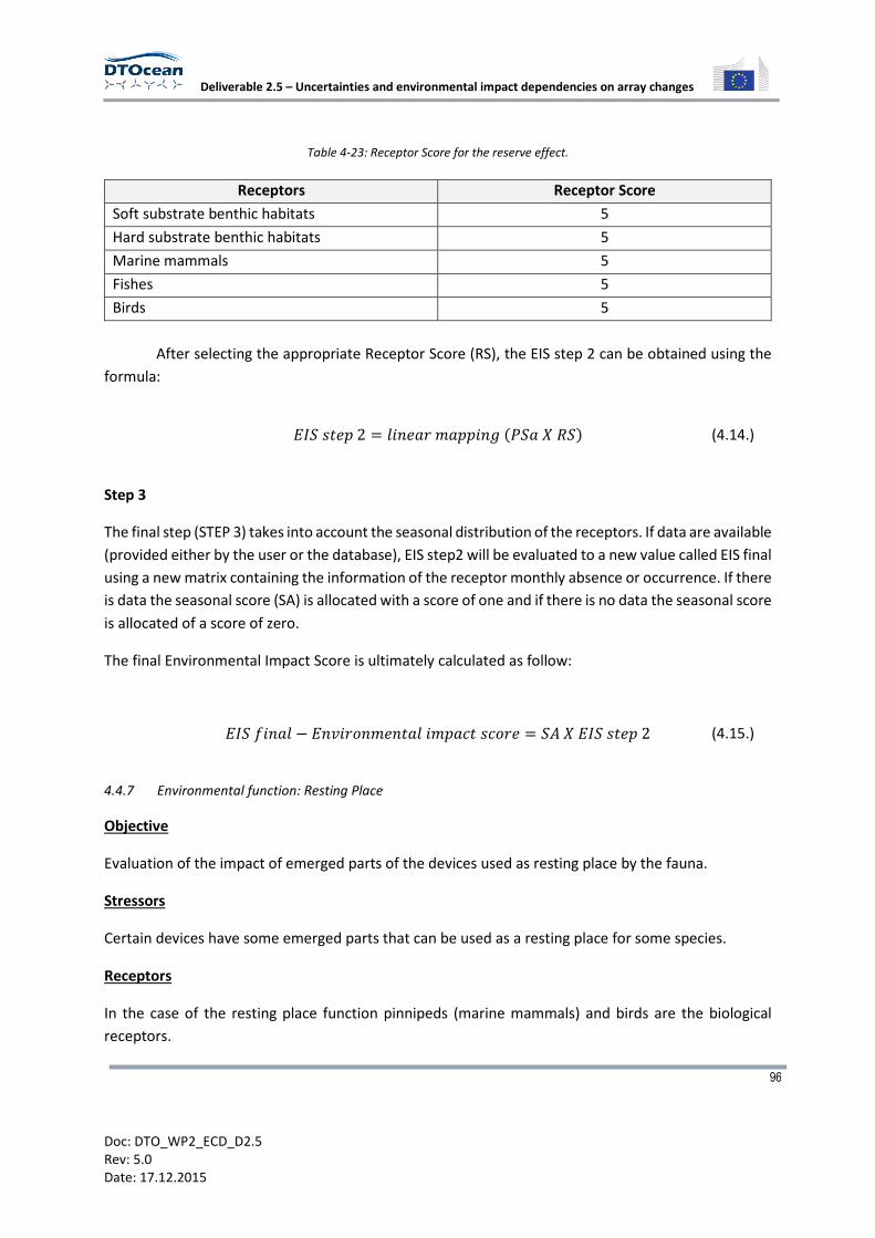
Deliverable 2.5 – Uncertainties and environmental impact dependencies on array changes
96
Doc: DTO_WP2_ECD_D2.5
Rev: 5.0
Date: 17.12.2015
Table 4-23: Receptor Score for the reserve effect.
Receptors Receptor Score
Soft substrate benthic habitats 5
Hard substrate benthic habitats 5
Marine mammals 5
Fishes 5
Birds 5
After selecting the appropriate Receptor Score (RS), the EIS step 2 can be obtained using the
formula:
2I�J94K2 � M6348-8KK630�N�8OP�� (4.14.)
Step 3
The final step (STEP 3) takes into account the seasonal distribution of the receptors. If data are available
(provided either by the user or the database), EIS step2 will be evaluated to a new value called EIS final
using a new matrix containing the information of the receptor monthly absence or occurrence. If there
is data the seasonal score (SA) is allocated with a score of one and if there is no data the seasonal score
is allocated of a score of zero.
The final Environmental Impact Score is ultimately calculated as follow:
2I�!638M � 23Q6-534398M6K879J75-4 � �RO2I�J94K2 (4.15.)
4.4.7 Environmental function: Resting Place
Objective
Evaluation of the impact of emerged parts of the devices used as resting place by the fauna.
Stressors
Certain devices have some emerged parts that can be used as a resting place for some species.
Receptors
In the case of the resting place function pinnipeds (marine mammals) and birds are the biological
receptors.

Deliverable 2.5 – Uncertainties and environmental impact dependencies on array changes
97
Doc: DTO_WP2_ECD_D2.5
Rev: 5.0
Date: 17.12.2015
Inputs
• surface area of the emerged part of the device
• number of device
• total of the surface lease area
Function’s formula
The 'reserve effect’ function is a ration between the fishery restriction surface and total of the lease
surface area.
P4J9630KM874
�
J_-!8748-485!9^444-041K8-95!9^414Q674O3_`4-5!14Q674J
9598MJ_-!874M48J48-48
(4.16.)
Rule
The impact increases with an increase of the surface area of the emerged parts of the devices.
Positive or negative impacts: depends on whether it is dangerous or not for the animals to stand on
these structures.
Weighting step
In the resting place function, the weighting step is linked to the dangerous part of devices.
4.4.7.1 Step 1
A resting place is considered as a positive effect and so the Pressure Score PS is positive. (Table 4-24).
• a low resting place for 0% to 10% recovery
• a moderate resting place for 10% to 30% recovery
• a high resting place for recovery between 30% and 70%
• a high resting place for a recovery higher than 70%
Table 4-24: Pressure Score Resting Place.
Resting place range PS - Pressure score fitting in resting place range
[0 -0,1] 1
[0,1-0,30[ 2

Deliverable 2.5 – Uncertainties and environmental impact dependencies on array changes
98
Doc: DTO_WP2_ECD_D2.5
Rev: 5.0
Date: 17.12.2015
[0,30-0,70] 3
>0.70 5
The resting place is defined in this report as a positive function, but this effect can be mitigated by the
presence of dangerous parts of a device such as traps and moving parts. It was decided to add a
weighting score based on this parameter (Table 4-25).
Table 4-25: Weighting Score for the resting place.
Dangerous Part of the devices WS-Weighting Score
No dangerous part of devices 1
blades 0.1
turbine shroud 0.1
oscillating water column with cavity 0.1
oscillating bodies with translation part 0.1
oscillating bodies with rotating part 0.1
flexible sleeve between each box (Pelamis) 0.1
At the end of this step the Pressure Score adjusted by the Weighting Score is calculated, the PSa the
Pressure Score Adjusted.
Step2
With environmental protection status, the majority of birds and all pinnipeds are protected. A specific
list of birds sensitive to resting places is expected to be available shortly. For now, RS is defined under
two categories (Table 4-26):
• General birds
• Pinnipeds
Table 4-26: Receptor Score for the resting place.
Species RS-Receptor Score
Birds 5
Pinnipeds 5
After selecting the appropriate Receptor Score (RS), the EIS step 2 can be obtained using the
formula.
2I�J94K2 � M6348-8KK630�N�8OP�� (4.17.)
Step 3
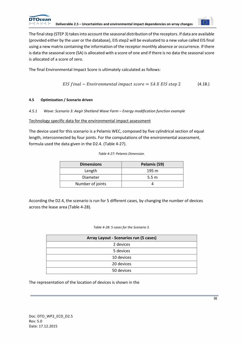
Deliverable 2.5 – Uncertainties and environmental impact dependencies on array changes
99
Doc: DTO_WP2_ECD_D2.5
Rev: 5.0
Date: 17.12.2015
The final step (STEP 3) takes into account the seasonal distribution of the receptors. If data are available
(provided either by the user or the database), EIS step2 will be evaluated to a new value called EIS final
using a new matrix containing the information of the receptor monthly absence or occurrence. If there
is data the seasonal score (SA) is allocated with a score of one and if there is no data the seasonal score
is allocated of a score of zero.
The final Environmental Impact Score is ultimately calculated as follows:
2I�!638M � 23Q6-534398M6K879J75-4 � �RO2I�J94K2 (4.18.)
4.5 Optimization / Scenario driven
4.5.1 Wave: Scenario 3: Aegir Shetland Wave Farm – Energy modification function example
Technology specific data for the environmental impact assessment
The device used for this scenario is a Pelamis WEC, composed by five cylindrical section of equal
length, interconnected by four joints. For the computations of the environmental assessment,
formula used the data given in the D2.4. (Table 4-27).
Table 4-27: Pelamis Dimension.
Dimensions Pelamis (59)
Length 195 m
Diameter 5.5 m
Number of joints 4
According the D2.4, the scenario is run for 5 different cases, by changing the number of devices
across the lease area (Table 4-28).
Table 4-28: 5 cases for the Scenario 3.
Array Layout - Scenarios run (5 cases)
2 devices
5 devices
10 devices
20 devices
50 devices
The representation of the location of devices is shown in the
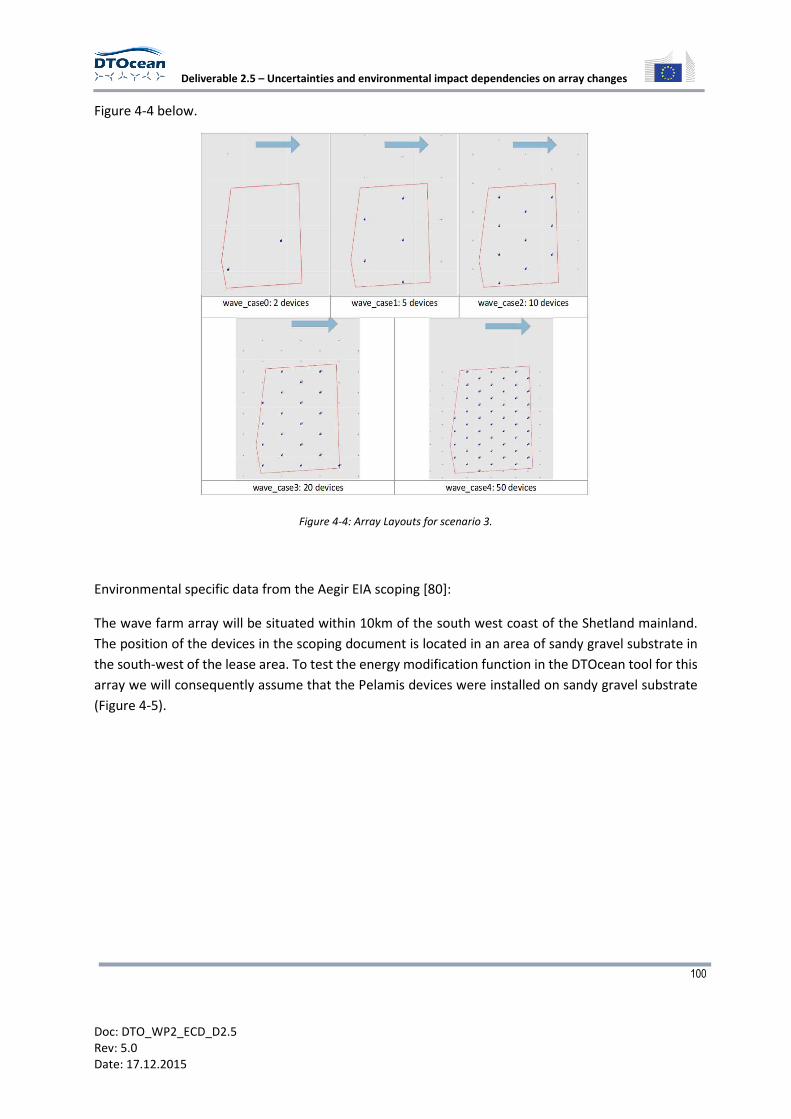
Deliverable 2.5 – Uncertainties and environmental impact dependencies on array changes
100
Doc: DTO_WP2_ECD_D2.5
Rev: 5.0
Date: 17.12.2015
Figure 4-4 below.
Figure 4-4: Array Layouts for scenario 3.
Environmental specific data from the Aegir EIA scoping [80]:
The wave farm array will be situated within 10km of the south west coast of the Shetland mainland.
The position of the devices in the scoping document is located in an area of sandy gravel substrate in
the south-west of the lease area. To test the energy modification function in the DTOcean tool for this
array we will consequently assume that the Pelamis devices were installed on sandy gravel substrate
(Figure 4-5).
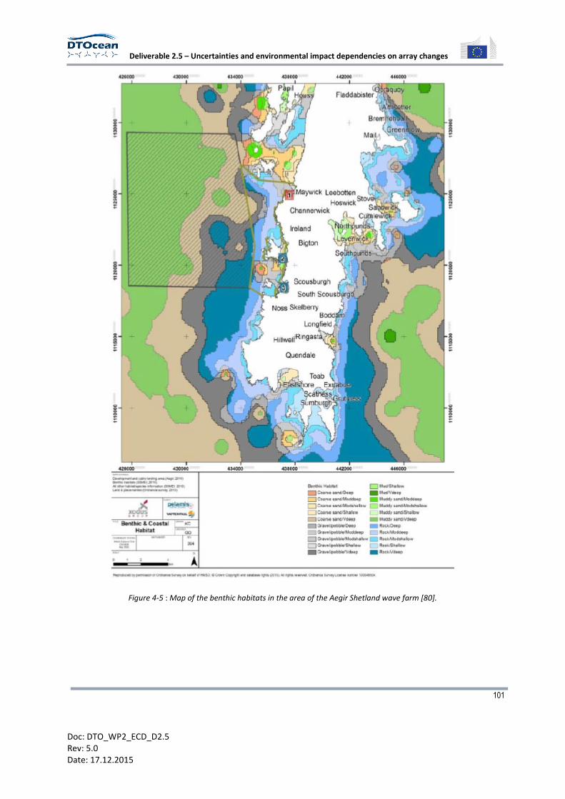
Deliverable 2.5 – Uncertainties and environmental impact dependencies on array changes
101
Doc: DTO_WP2_ECD_D2.5
Rev: 5.0
Date: 17.12.2015
Figure 4-5 : Map of the benthic habitats in the area of the Aegir Shetland wave farm [80].
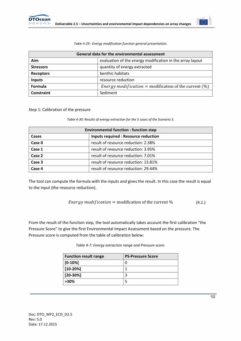
Deliverable 2.5 – Uncertainties and environmental impact dependencies on array changes
102
Doc: DTO_WP2_ECD_D2.5
Rev: 5.0
Date: 17.12.2015
Table 4-29 : Energy modification function general presentation.
General data for the environmental assessment
Aim evaluation of the energy modification in the array layout
Stressors quantity of energy extracted
Receptors benthic habitats
Inputs resource reduction
Formula 234-0�516!6789653 � modificationofthecurrent�%�
Constraint Sediment
Step 1: Calibration of the pressure
Table 4-30: Results of energy extraction for the 5 cases of the Scenario 3.
Environmental function : function step
Cases Inputs required : Resource reduction
Case 0 result of resource reduction: 2.38%
Case 1 result of resource reduction: 3.95%
Case 2 result of resource reduction: 7.01%
Case 3 result of resource reduction: 13.81%
Case 4 result of resource reduction: 29.44%
The tool can compute the formula with the inputs and gives the result. In this case the result is equal
to the input (the resource reduction).
234-0�516!6789653 � modificationofthecurrent% (4.1.)
From the result of the function step, the tool automatically takes account the first calibration “the
Pressure Score” to give the first Environmental Impact Assessment based on the pressure. The
Pressure score is computed from the table of calibration below:
Table 4-7: Energy extraction range and Pressure score.
Function result range PS-Pressure Score
[0-10%[ 0
[10-20%( 1
[20-30%] 3
>30% 5
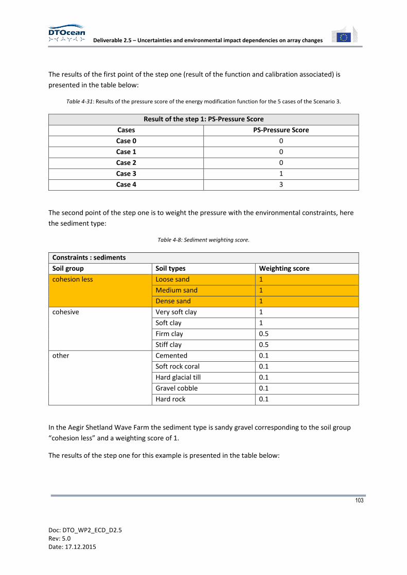
Deliverable 2.5 – Uncertainties and environmental impact dependencies on array changes
103
Doc: DTO_WP2_ECD_D2.5
Rev: 5.0
Date: 17.12.2015
The results of the first point of the step one (result of the function and calibration associated) is
presented in the table below:
Table 4-31: Results of the pressure score of the energy modification function for the 5 cases of the Scenario 3.
Result of the step 1: PS-Pressure Score
Cases PS-Pressure Score
Case 0 0
Case 1 0
Case 2 0
Case 3 1
Case 4 3
The second point of the step one is to weight the pressure with the environmental constraints, here
the sediment type:
Table 4-8: Sediment weighting score.
Constraints : sediments
Soil group Soil types Weighting score
cohesion less Loose sand 1
Medium sand 1
Dense sand 1
cohesive Very soft clay 1
Soft clay 1
Firm clay 0.5
Stiff clay 0.5
other Cemented 0.1
Soft rock coral 0.1
Hard glacial till 0.1
Gravel cobble 0.1
Hard rock 0.1
In the Aegir Shetland Wave Farm the sediment type is sandy gravel corresponding to the soil group
“cohesion less” and a weighting score of 1.
The results of the step one for this example is presented in the table below:
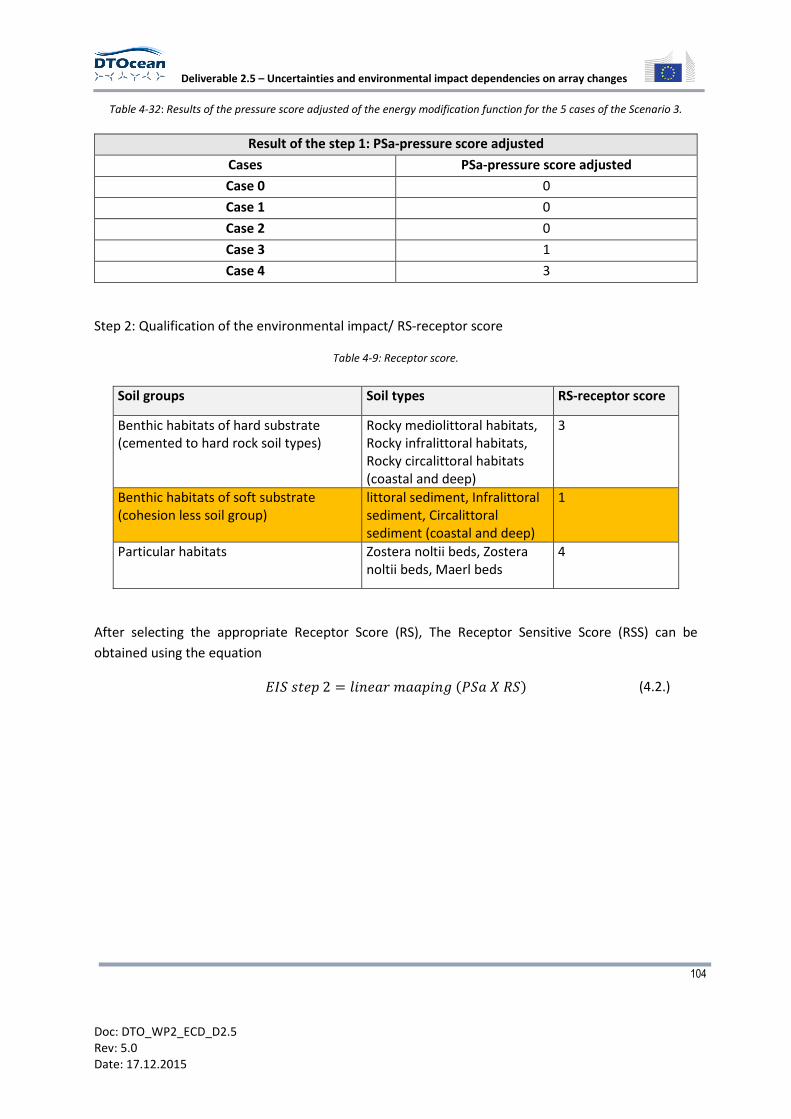
Deliverable 2.5 – Uncertainties and environmental impact dependencies on array changes
104
Doc: DTO_WP2_ECD_D2.5
Rev: 5.0
Date: 17.12.2015
Table 4-32: Results of the pressure score adjusted of the energy modification function for the 5 cases of the Scenario 3.
Result of the step 1: PSa-pressure score adjusted
Cases PSa-pressure score adjusted
Case 0 0
Case 1 0
Case 2 0
Case 3 1
Case 4 3
Step 2: Qualification of the environmental impact/ RS-receptor score
Table 4-9: Receptor score.
Soil groups Soil types RS-receptor score
Benthic habitats of hard substrate
(cemented to hard rock soil types)
Rocky mediolittoral habitats,
Rocky infralittoral habitats,
Rocky circalittoral habitats
(coastal and deep)
3
Benthic habitats of soft substrate
(cohesion less soil group)
littoral sediment, Infralittoral
sediment, Circalittoral
sediment (coastal and deep)
1
Particular habitats Zostera noltii beds, Zostera
noltii beds, Maerl beds
4
After selecting the appropriate Receptor Score (RS), The Receptor Sensitive Score (RSS) can be
obtained using the equation
2I�J94K2 � M6348-88K630�N�8OP�� (4.2.)
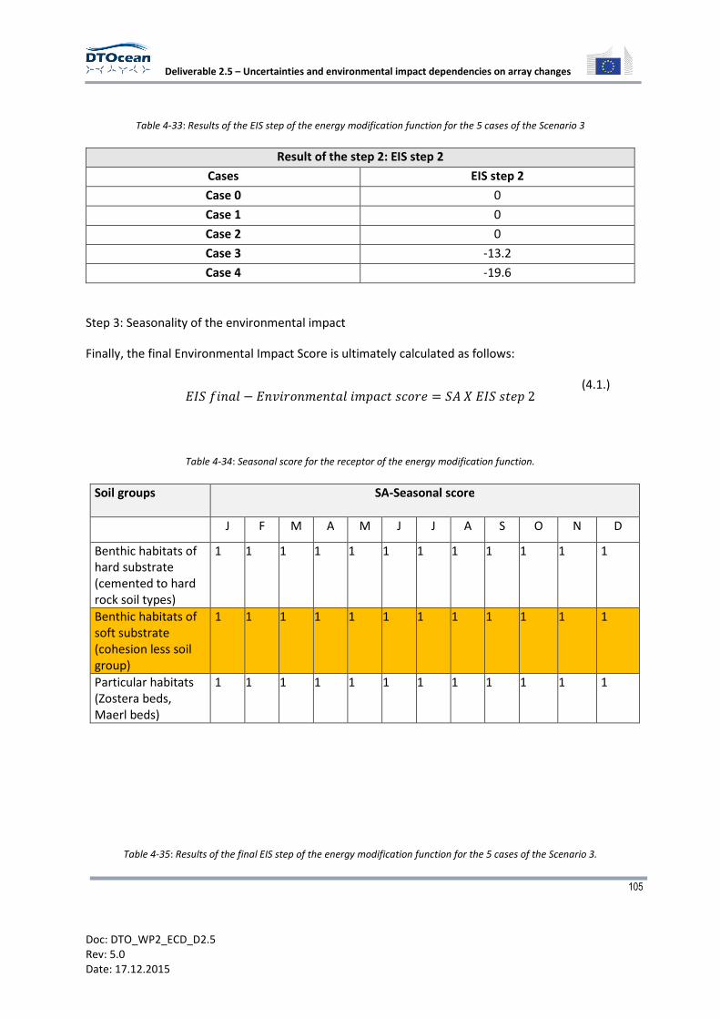
Deliverable 2.5 – Uncertainties and environmental impact dependencies on array changes
105
Doc: DTO_WP2_ECD_D2.5
Rev: 5.0
Date: 17.12.2015
Table 4-33: Results of the EIS step of the energy modification function for the 5 cases of the Scenario 3
Result of the step 2: EIS step 2
Cases EIS step 2
Case 0 0
Case 1 0
Case 2 0
Case 3 -13.2
Case 4 -19.6
Step 3: Seasonality of the environmental impact
Finally, the final Environmental Impact Score is ultimately calculated as follows:
2I�!638M � 23Q6-534398M6K879J75-4 � �RO2I�J94K2
(4.1.)
Table 4-34: Seasonal score for the receptor of the energy modification function.
Soil groups SA-Seasonal score
J F M A M J J A S O N D
Benthic habitats of
hard substrate
(cemented to hard
rock soil types)
1 1 1 1 1 1 1 1 1 1 1 1
Benthic habitats of
soft substrate
(cohesion less soil
group)
1 1 1 1 1 1 1 1 1 1 1 1
Particular habitats
(Zostera beds,
Maerl beds)
1 1 1 1 1 1 1 1 1 1 1 1
Table 4-35: Results of the final EIS step of the energy modification function for the 5 cases of the Scenario 3.
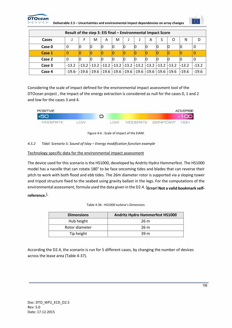
Deliverable 2.5 – Uncertainties and environmental impact dependencies on array changes
106
Doc: DTO_WP2_ECD_D2.5
Rev: 5.0
Date: 17.12.2015
Result of the step 3: EIS final – Environmental Impact Score
Cases J F M A M J J A S O N D
Case 0 0 0 0 0 0 0 0 0 0 0 0 0
Case 1 0 0 0 0 0 0 0 0 0 0 0 0
Case 2 0 0 0 0 0 0 0 0 0 0 0 0
Case 3 -13.2 -13.2 -13.2 -13.2 -13.2 -13.2 -13.2 -13.2 -13.2 -13.2 -13.2 -13.2
Case 4 -19.6- -19.6 -19.6 -19.6 -19.6 -19.6 -19.6 -19.6 -19.6 -19.6 -19.6 -19.6
Considering the scale of impact defined for the environmental impact assessment tool of the
DTOcean project , the impact of the energy extraction is considered as null for the cases 0, 1 and 2
and low for the cases 3 and 4.
Figure 4-6 : Scale of impact of the EIAM.
4.5.2 Tidal: Scenario 5: Sound of Islay – Energy modification function example
Technology specific data for the environmental impact assessment
The device used for this scenario is the HS1000, developed by Andritz Hydro Hammerfest. The HS1000
model has a nacelle that can rotate 180° to be face oncoming tides and blades that can reverse their
pitch to work with both flood and ebb tides. The 26m diameter rotor is supported via a sloping tower
and tripod structure fixed to the seabed using gravity ballast in the legs. For the computations of the
environmental assessment, formula used the data given in the D2.4. (Error! Not a valid bookmark self-
reference.).
Table 4-36 : HS1000 turbine’s Dimension.
Dimensions Andritz Hydro Hammerfest HS1000
Hub height 26 m
Rotor diameter 26 m
Tip height 39 m
According the D2.4, the scenario is run for 5 different cases, by changing the number of devices
across the lease area (Table 4-37).
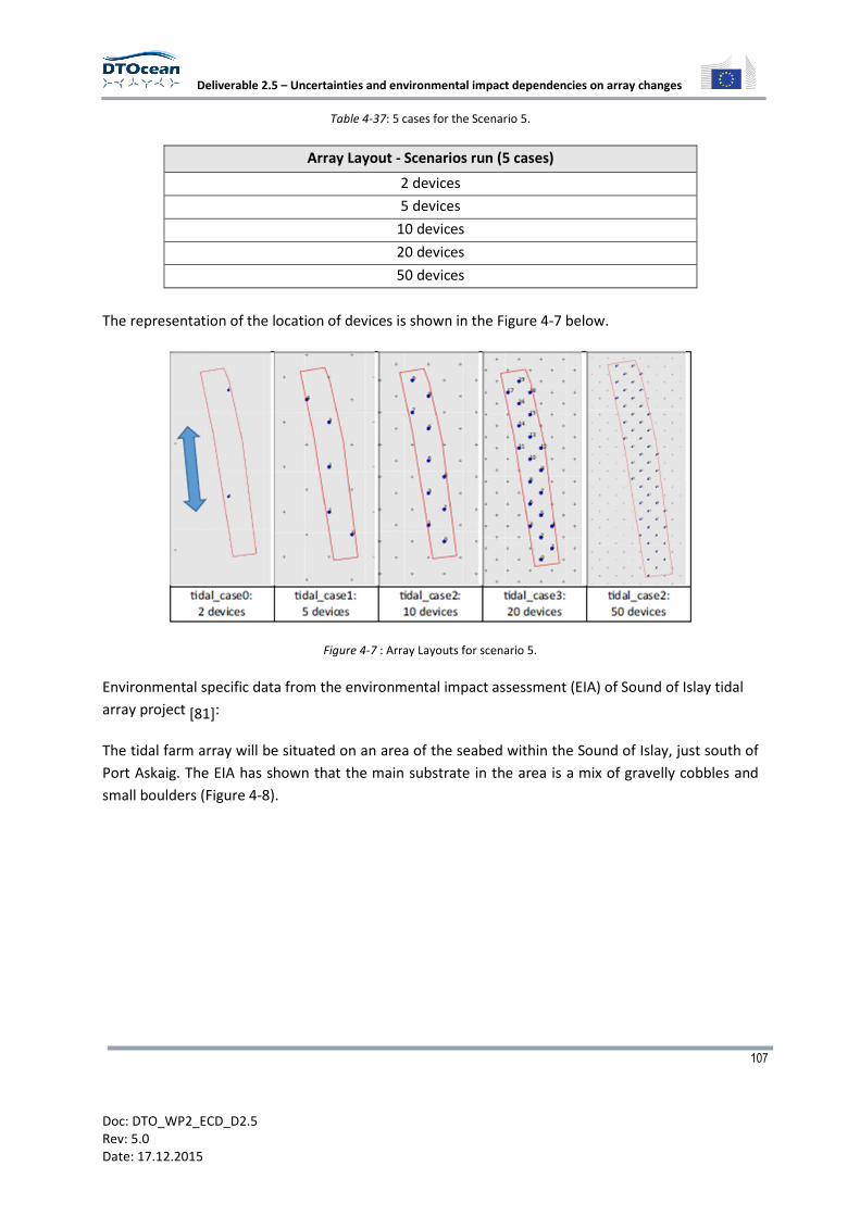
Deliverable 2.5 – Uncertainties and environmental impact dependencies on array changes
107
Doc: DTO_WP2_ECD_D2.5
Rev: 5.0
Date: 17.12.2015
Table 4-37: 5 cases for the Scenario 5.
Array Layout - Scenarios run (5 cases)
2 devices
5 devices
10 devices
20 devices
50 devices
The representation of the location of devices is shown in the Figure 4-7 below.
Figure 4-7 : Array Layouts for scenario 5.
Environmental specific data from the environmental impact assessment (EIA) of Sound of Islay tidal
array project [81]:
The tidal farm array will be situated on an area of the seabed within the Sound of Islay, just south of
Port Askaig. The EIA has shown that the main substrate in the area is a mix of gravelly cobbles and
small boulders (Figure 4-8).
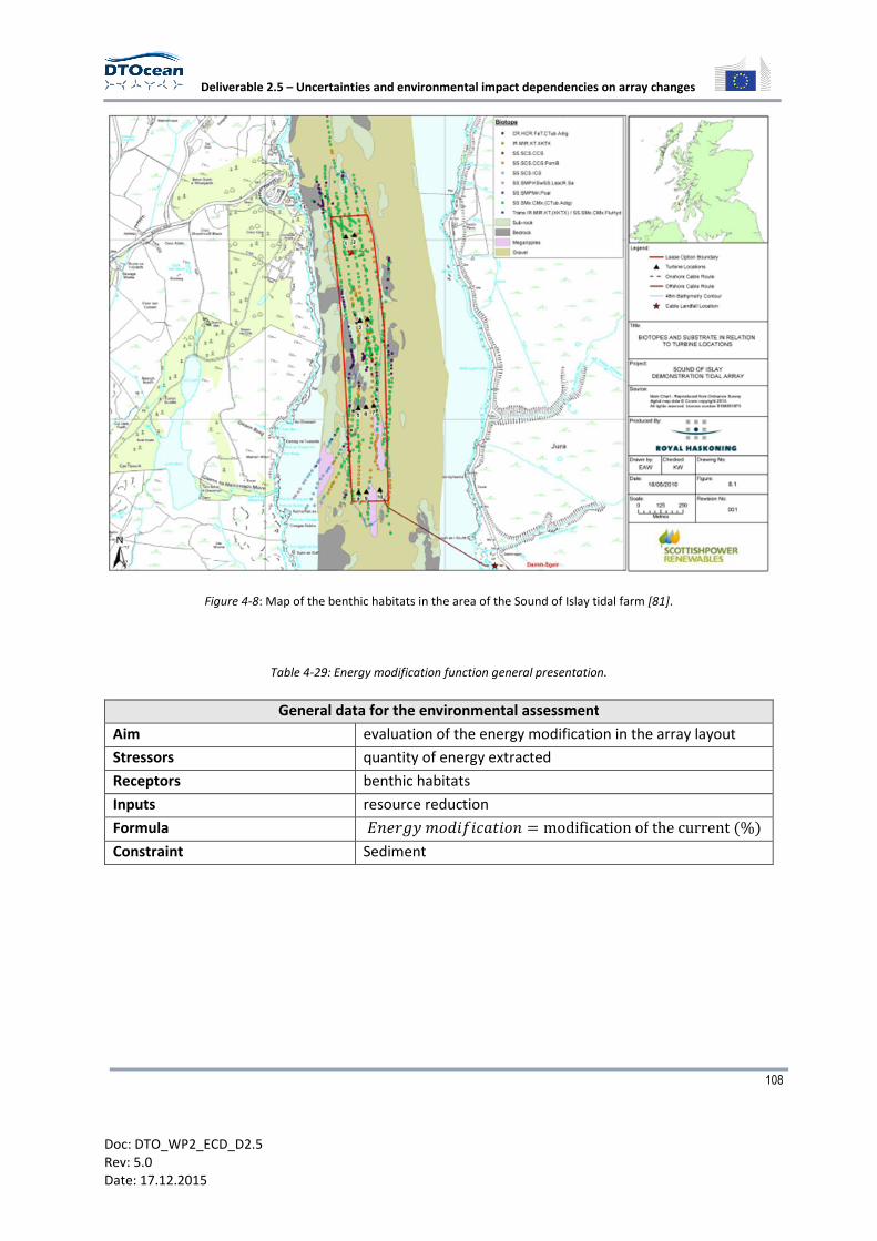
Deliverable 2.5 – Uncertainties and environmental impact dependencies on array changes
108
Doc: DTO_WP2_ECD_D2.5
Rev: 5.0
Date: 17.12.2015
Figure 4-8: Map of the benthic habitats in the area of the Sound of Islay tidal farm [81].
Table 4-29: Energy modification function general presentation.
General data for the environmental assessment
Aim evaluation of the energy modification in the array layout
Stressors quantity of energy extracted
Receptors benthic habitats
Inputs resource reduction
Formula 234-0�516!6789653 � modificationofthecurrent�%�
Constraint Sediment
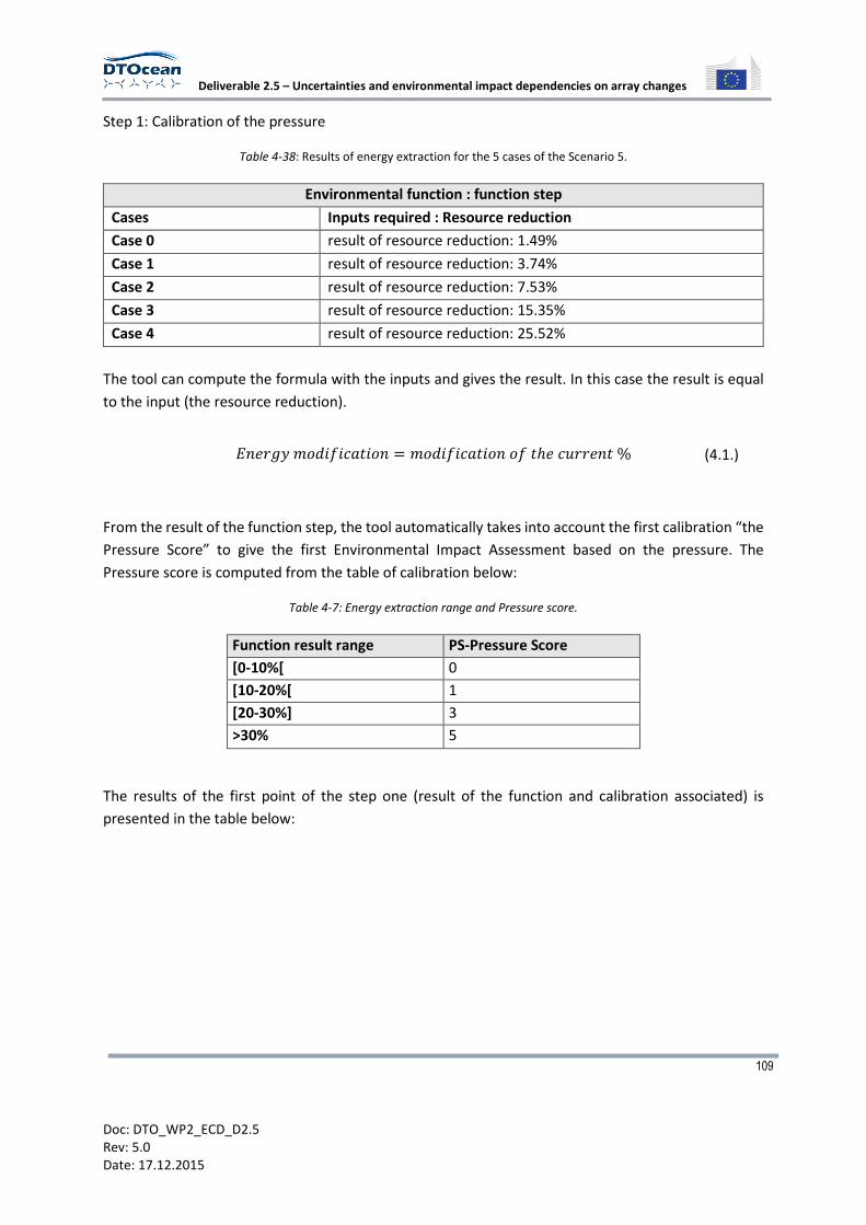
Deliverable 2.5 – Uncertainties and environmental impact dependencies on array changes
109
Doc: DTO_WP2_ECD_D2.5
Rev: 5.0
Date: 17.12.2015
Step 1: Calibration of the pressure
Table 4-38: Results of energy extraction for the 5 cases of the Scenario 5.
Environmental function : function step
Cases Inputs required : Resource reduction
Case 0 result of resource reduction: 1.49%
Case 1 result of resource reduction: 3.74%
Case 2 result of resource reduction: 7.53%
Case 3 result of resource reduction: 15.35%
Case 4 result of resource reduction: 25.52%
The tool can compute the formula with the inputs and gives the result. In this case the result is equal
to the input (the resource reduction).
234-0�516!6789653 � 516!67896535!9^47_--439% (4.1.)
From the result of the function step, the tool automatically takes into account the first calibration “the
Pressure Score” to give the first Environmental Impact Assessment based on the pressure. The
Pressure score is computed from the table of calibration below:
Table 4-7: Energy extraction range and Pressure score.
Function result range PS-Pressure Score
[0-10%[ 0
[10-20%[ 1
[20-30%] 3
>30% 5
The results of the first point of the step one (result of the function and calibration associated) is
presented in the table below:
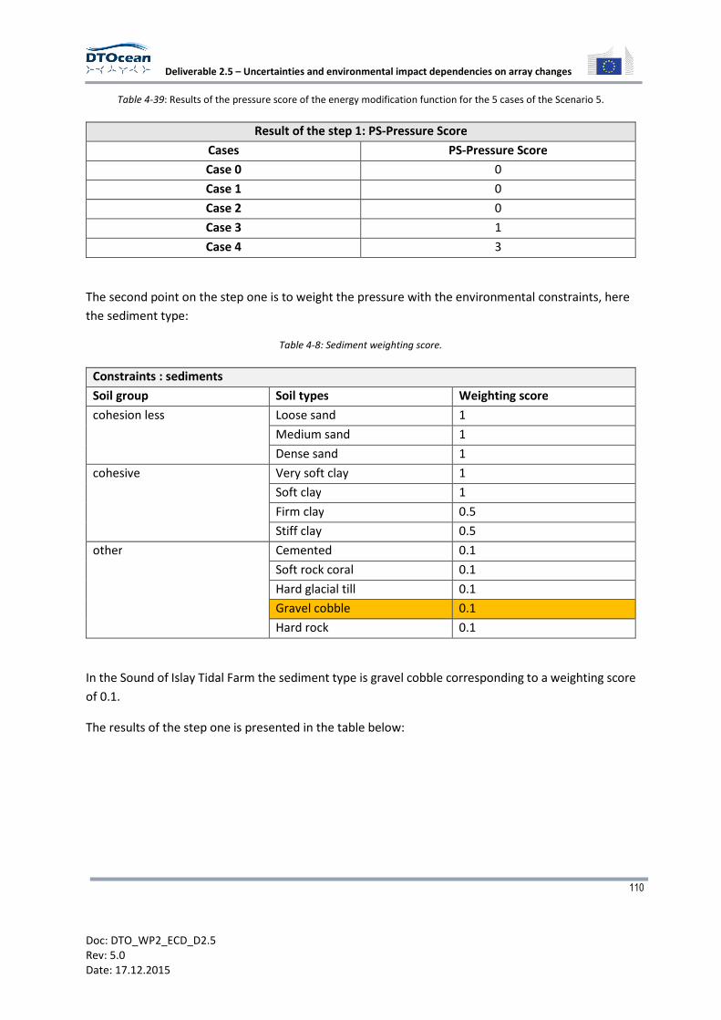
Deliverable 2.5 – Uncertainties and environmental impact dependencies on array changes
110
Doc: DTO_WP2_ECD_D2.5
Rev: 5.0
Date: 17.12.2015
Table 4-39: Results of the pressure score of the energy modification function for the 5 cases of the Scenario 5.
Result of the step 1: PS-Pressure Score
Cases PS-Pressure Score
Case 0 0
Case 1 0
Case 2 0
Case 3 1
Case 4 3
The second point on the step one is to weight the pressure with the environmental constraints, here
the sediment type:
Table 4-8: Sediment weighting score.
Constraints : sediments
Soil group Soil types Weighting score
cohesion less Loose sand 1
Medium sand 1
Dense sand 1
cohesive Very soft clay 1
Soft clay 1
Firm clay 0.5
Stiff clay 0.5
other Cemented 0.1
Soft rock coral 0.1
Hard glacial till 0.1
Gravel cobble 0.1
Hard rock 0.1
In the Sound of Islay Tidal Farm the sediment type is gravel cobble corresponding to a weighting score
of 0.1.
The results of the step one is presented in the table below:
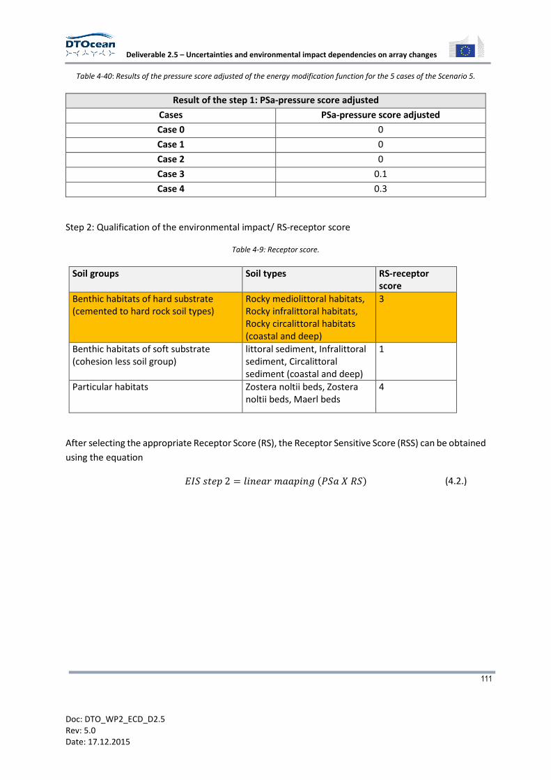
Deliverable 2.5 – Uncertainties and environmental impact dependencies on array changes
111
Doc: DTO_WP2_ECD_D2.5
Rev: 5.0
Date: 17.12.2015
Table 4-40: Results of the pressure score adjusted of the energy modification function for the 5 cases of the Scenario 5.
Result of the step 1: PSa-pressure score adjusted
Cases PSa-pressure score adjusted
Case 0 0
Case 1 0
Case 2 0
Case 3 0.1
Case 4 0.3
Step 2: Qualification of the environmental impact/ RS-receptor score
Table 4-9: Receptor score.
Soil groups Soil types RS-receptor
score
Benthic habitats of hard substrate
(cemented to hard rock soil types)
Rocky mediolittoral habitats,
Rocky infralittoral habitats,
Rocky circalittoral habitats
(coastal and deep)
3
Benthic habitats of soft substrate
(cohesion less soil group)
littoral sediment, Infralittoral
sediment, Circalittoral
sediment (coastal and deep)
1
Particular habitats Zostera noltii beds, Zostera
noltii beds, Maerl beds
4
After selecting the appropriate Receptor Score (RS), the Receptor Sensitive Score (RSS) can be obtained
using the equation
2I�J94K2 � M6348-88K630�N�8OP�� (4.2.)
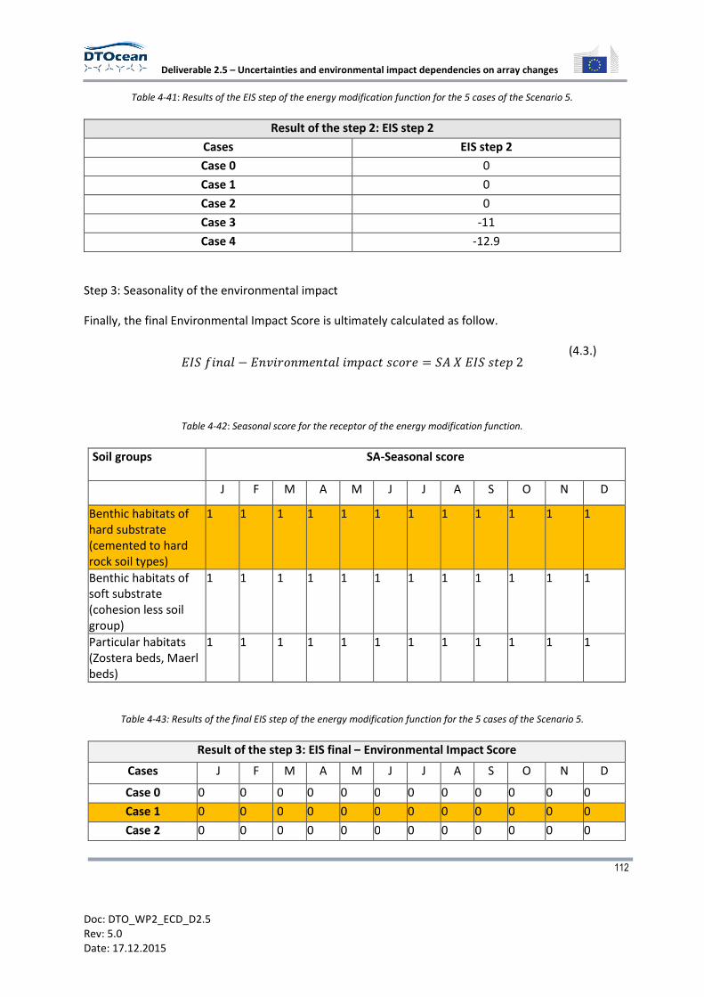
Deliverable 2.5 – Uncertainties and environmental impact dependencies on array changes
112
Doc: DTO_WP2_ECD_D2.5
Rev: 5.0
Date: 17.12.2015
Table 4-41: Results of the EIS step of the energy modification function for the 5 cases of the Scenario 5.
Result of the step 2: EIS step 2
Cases EIS step 2
Case 0 0
Case 1 0
Case 2 0
Case 3 -11
Case 4 -12.9
Step 3: Seasonality of the environmental impact
Finally, the final Environmental Impact Score is ultimately calculated as follow.
2I�!638M � 23Q6-534398M6K879J75-4 � �RO2I�J94K2
(4.3.)
Table 4-42: Seasonal score for the receptor of the energy modification function.
Soil groups SA-Seasonal score
J F M A M J J A S O N D
Benthic habitats of
hard substrate
(cemented to hard
rock soil types)
1 1 1 1 1 1 1 1 1 1 1 1
Benthic habitats of
soft substrate
(cohesion less soil
group)
1 1 1 1 1 1 1 1 1 1 1 1
Particular habitats
(Zostera beds, Maerl
beds)
1 1 1 1 1 1 1 1 1 1 1 1
Table 4-43: Results of the final EIS step of the energy modification function for the 5 cases of the Scenario 5.
Result of the step 3: EIS final – Environmental Impact Score
Cases J F M A M J J A S O N D
Case 0 0 0 0 0 0 0 0 0 0 0 0 0
Case 1 0 0 0 0 0 0 0 0 0 0 0 0
Case 2 0 0 0 0 0 0 0 0 0 0 0 0

Deliverable 2.5 – Uncertainties and environmental impact dependencies on array changes
113
Doc: DTO_WP2_ECD_D2.5
Rev: 5.0
Date: 17.12.2015
Case 3 -11 -11 -11 -11 -11 -11 -11 -11 -11 -11 -11 -11
Case 4 -12.9 -12.9 -
12.9
-12.9 -12.9 -12.9 -12.9 -12.9 -12.9 -12.9 -12.9 -12.9
Considering the scale of impact defined for the environmental impact assessment tool of the
DTOcean project, the impact of the energy extraction is considered as null for the cases 0, 1 and 2
and low for the cases 3 and 4.
Figure 4-9 : Scale of impact of the EIAM.

Deliverable 2.5 – Uncertainties and environmental impact dependencies on array changes
114
Doc: DTO_WP2_ECD_D2.5
Rev: 5.0
Date: 17.12.2015
5 GENERAL CONCLUSION
In terms of environmental impacts and dependencies on array changes, energy extraction and collision
risks are two of the main concerns. Energy extraction can potentially modify sediment transport due
to alteration of hydraulics and hydrologic regimes that may reduce the ability of streams to transport
sediment and debris, causing deposition of suspended sediments and thereby alter bottom habitats.
This can then generate habitat loss, smothering or contamination that directly affects benthic habitats.
The impact on perturbations of the water flow and their consequences on sedimentary processes are
expected to be much less significant for wave than for tidal energy converters. Collision risks are also
directly related to array changes. Currently, collision risks related to wave and tidal devices are still
poorly understood due to a lack of installed tidal and wave devices. For birds, collision risks may be
mainly related to diving depth attained in the water column, swimming speed, the diurnal rhythm of
foraging, location and behavior of species, and sea state in terms of turbidity and water flow. For
marine mammals, entanglement is also considered. Overall the risk of collision is in part a function of
the mammal’s species, but also the body size, swimming behavior and skills, capacity to detect devices
as well as the device type. Therefore, the design of devices and array organization are important in
preventing collisions and entanglements.
Other impacts considered here include underwater noise, chemical pollution risk, resting places, reef
effects and reserve effects. Within the framework of DTOcean, environmental impacts are described
through a set of functions that constitute the foundations of the Environmental Impact Assessment
Module (EIAM), the purpose of which is to globally assess the environmental impacts generated by the
various technological choices to optimize an array of wave or tidal devices. General and specific (based
on scenario) recommendations have been proposed for each impact. However, due to the lack of data
and feedback from recent developments, these recommendations should be taken with caution.
Besides, little is known about the long term effects. As knowledge about environmental impacts will
progress in the coming years of MRE array development, the DTOcean EIAM will be able to be updated,
thanks to its open source policy, in order to better assess environmental impacts.
Deliverable 2.5 – Uncertainties and environmental impact dependencies on array changes
115
Doc: DTO_WP2_ECD_D2.5
Rev: 5.0
Date: 17.12.2015
6 REFERENCES
[1] DHI, Mike 21 User Manuel. 2011. [2] M. . Longuet-Higgins, “On the joint distribution of the periods and amplitudes of sea
waves,” J. Geophys. Res., no. 80, pp. 2688–2694, 1975. [3] Det Norske Veritas, “Environmental Conditions and Environmental Loads: DNV-RP-
C205,” DNV-RP-C205, 2010. [4] J. Cruz, Ocean Wave Energy, Current Status and Future Perspective, Springer. . [5] IEC TS 62600-101, “Wave, tidal and other water current converters,” Mar. Energy. [6] L. Zhou and P. Frigaard, “Generation and Analysis of Random Waves,” 2001. [7] DTOcean Project, “DTOcean, Deliverable 1.1, ‘Detailed deployment scenarios for wave
and tidal energy converters’,” 2014. [8] DTOcean Project, “Deliverable 2.2, “Pre-evaluation of array layouts, identified key
parameters and their relevant ranges,” 2014. [9] G. Yoshimi, Random Seas and Design of Maritime Structures, World Scientific. . [10] N. Kottegoda and R. Rosso, Applied Statitiscs for Civil and Environmental Engineers.
Blackwell Publishing, 2008. [11] I. Katic, J. Hojstrup, and N. . Jensen, “A Simple Model for Cluster Efficiency. In Proc.
of the BWEA Conference,” 1986, pp. 407–410. [12] G. . Larsen, A Simple Wake Calculation Procedure. 1988. [13] G. Habenicht, . Comparison of Different Wake Combination Methods for Offshore Wake
Modelling. 2008. [14] T. Burton, Wind Energy Handbook, 2nd Edition, 2nd ed. 2011. [15] J. . Whelan, “Modelling of Free Surface Proximity and Wave Induced Velocities around
an Horizontal Axis Tidal Stream Turbine. In 7th European Wave and Tidal Energy Conference,” Porto, 2007.
[16] M. . Thomson and D. McCowen, WG3WP4 D1 GH BLOCKAGE MODELLING. 2010. [17] S. C. James, E. Seetho, C. Jones, and J. Roberts, “Simulating environmental changes due
to marine hydrokinetic energy installations,” OCEANS 2010, pp. 1–10, 2010. [18] US Department of Energy, “Report to Congress on the potential environmental effects of
marine and hydrokinetic energy technologies,” 2009. [19] M. A. Shields, D. K. Woolf, E. P. Grist, S. A. Kerr, A. Jackson, R. E. Harris, M. C. Bell,
R. Beharie, A. Want, E. Osalusi, and others, “Marine renewable energy: the ecological implications of altering the hydrodynamics of the marine environment,” Ocean Coast. Manag., vol. 54, no. 1, pp. 2–9, 2011.
[20] C. Frid, E. Andonegi, J. Depestele, A. Judd, D. Rihan, S. I. Rogers, and E. Kenchington, “The environmental interactions of tidal and wave energy generation devices,” Environ. Impact Assess. Rev., vol. 32, no. 1, pp. 133–139, 2012.
[21] G. Saunders, G. . Bedford, J. . Trendall, and I. Sotheran, “Guidance on Survey and Monitoring in Relation to Marine Renewables Deployments in Scotland Volume 3: Seals,” Scottish Natural Heritage and Marine Scotland, 2011.
[22] M. Lejart, M. Boeuf, A. Barillier, J.-M. Loaec, C. Giry, J. Prevot, C. Auvray, T. Folegot, A. Carlier, J.-P. Delpech, L. Martinez, and B. Cadiou, “Guide to the environmental impact evaluation of tidal stream technologies at sea : GHYDRO,” France Energies Marines, 2013.
Deliverable 2.5 – Uncertainties and environmental impact dependencies on array changes
116
Doc: DTO_WP2_ECD_D2.5
Rev: 5.0
Date: 17.12.2015
[23] G. Cada, J. Ahlgrimm, M. Bahleda, T. Bigford, S. D. Stavrakas, D. Hall, R. Moursund, and M. Sale, “Potential impacts of hydrokinetic and wave energy conversion technologies on aquatic environments,” Fisheries, vol. 32, no. 4, pp. 174–181, 2007.
[24] C. Frid, E. Andonegi, J. Depestele, A. Judd, D. Rihan, S. I. Rogers, and E. Kenchington, “The environmental interactions of tidal and wave energy generation devices,” Environ. Impact Assess. Rev., vol. 32, no. 1, pp. 133–139, 2012.
[25] Widdows and Brinsley, 2002. [26] M. Kadiri, R. Ahmadian, B. Bockelmann-Evans, W. Rauen, and R. Falconer, “A review
of the potential water quality impacts of tidal renewable energy systems,” Renew. Sustain. Energy Rev., vol. 16, no. 1, pp. 329–341, 2012.
[27] P. E. Robins, S. P. Neill, and M. J. Lewis, “Impact of tidal-stream arrays in relation to the natural variability of sedimentary processes,” Renew. Energy, vol. 72, pp. 311–321, 2014.
[28] B. Wilson, R. Batty, F. Daunt, and C. Carter, “Collision risks between marine renewable energy devices and mammals, fish and diving birds: Report to the Scottish Executive,” 2006.
[29] Bicknell, Votier, Inger, and Atrill, “‘ The impact of marine renewable energy on birds’.,” Mar. Renew. Biodivers. Fish. Mar. Inst., pp. 22–25, 2013.
[30] K.-M. Exo, O. Huppop, and S. Garthe, “Birds and offshore wind farms: a hot topic in marine ecology,” Bull.-Wader Study Group, vol. 100, pp. 50–53, 2003.
[31] Langton, Davies, and Scott, “Seabird conservation and tidal stream and wave power generation: Information needs for predicting and manging potential impacts.,” Marine Policy, Aberdeen, p. 8, 2011.
[32] W. J. Grecian, R. Inger, M. J. Attrill, S. Bearhop, B. J. Godley, M. J. Witt, and S. C. Votier, “Potential impacts of wave-powered marine renewable energy installations on marine birds,” Ibis, vol. 152, no. 4, pp. 683–697, 2010.
[33] S. Dolman and M. Simmonds, “Towards best environmental practice for cetacean conservation in developing Scotland’s marine renewable energy,” Mar. Policy, vol. 34, no. 5, pp. 1021–1027, 2010.
[34] C. Sparling, M. Lonergan, B. Mackey, C. Booth, G. Hastie, D. Gillespie, and J. MacAulay, “Marine Mammals and Tidal Turbines: Understanding true collision risk.”
[35] S. Benjamins, V. Harnois, H. Smith, L. Greenhill, L. Johanning, C. Carter, and B. Wilson, “Understanding the potential for marine megafauna entanglement risk from renewable marine energy developments.,” Scottish Natural Heritage Commissioned Report, 791, 2014.
[36] R. Inger, M. Attrill, S. Bearhop, A. Broderick, W. James Grecian, D. Hodgson, C. Mills, E. Sheehan, S. Votier, and M. Witt, “Marine renewable energy: potential benefits to biodiversity? An urgent call for research.,” J Appl Ecol, vol. 46(6), pp. 1145–1153, 2009.
[37] Carter, Wilson, and Black, “Marine renewable energy devices: a collision risk for marine mammals? Proceedings of the ASCOBANS/ECS workshop: offshore wind farms and marine mammals: impacts & methodologies for assessing impacts. San Sebastian,” ECS special publication series, Spain, 2008.
[38] G. Keenan, C. Sparling, H. Williams, and F. Fortune, “SeaGen Environmental Monitoring Programme Final Report,” Royal Haskoning, 2011.
Deliverable 2.5 – Uncertainties and environmental impact dependencies on array changes
117
Doc: DTO_WP2_ECD_D2.5
Rev: 5.0
Date: 17.12.2015
[39] M. Baeye and M. Fettweis, “In situ observations of suspended particulate matter plumes at an offshore wind farm, southern North Sea,” Geo-Mar. Lett., pp. 1–9, 2015.
[40] J. E. Cloern, “Turbidity as a control on phytoplankton biomass and productivity in estuaries,” Cont. Shelf Res., vol. 7, no. 11, pp. 1367–1381, 1987.
[41] V. L. Todd, I. B. Todd, J. C. Gardiner, E. C. Morrin, N. A. MacPherson, N. A. DiMarzio, and F. Thomsen, “A review of impacts of marine dredging activities on marine mammals,” ICES J. Mar. Sci. J. Cons., vol. 72, no. 2, pp. 328–340, 2015.
[42] T. Strod, Z. Arad, I. Izhaki, and G. Katzir, “Cormorants keep their power: visual resolution in a pursuit-diving bird under amphibious and turbid conditions,” Curr. Biol., vol. 14, no. 10, pp. R376–R377, 2004.
[43] H. Tillin, J. Hiddink, S. Jennings, and M. Kaiser, “Chronic bottom trawling alters the functional composition of benthic invertebrate communities on a sea-basin scale,” Mar. Ecol. Prog. Ser., vol. 318, pp. 31–45, 2006.
[44] S. . Robinson and P. . Lepper, “Scoping sudy: review of current knowledge of underwater noise emissions from wave and tidal stream energy devices.,” The Crown Estate, 2013.
[45] D. R. Ketten, “Marine mammal auditory systems: a summary of audiometric and anatomical data and implications for underwater acoustic impacts,” Polarforschung, vol. 72, no. 2/3, pp. 79–92, 2004.
[46] J. Nedwell, A. Brooker, and R. BArham, “Assessment of underwater noise during the installation of export power cables at the Beatrice Offshore Wind Farm. Subacoustech Environmental Report.,” Subacoustech Environmental, E318R0106, 2012.
[47] M. . Commission, “Marine mammals and noise: a sound approach to research and management,” Report to Congress from the Marine Mammal Commission, 2007.
[48] W. W. Clark, “Recent studies of temporary threshold shift (TTS) and permanent threshold shift (PTS) in animals,” J. Acoust. Soc. Am., vol. 90, no. 1, pp. 155–163, 1991.
[49] A. B. Gill and M. D. Bartlett, “Literature review on the potential effects of electromagnetic fields and subsea noise from marine renewable energy developments on Atlantic salmon, sea trout and European eel. Scottish Natural Heritage Commissioned Report,” 2010.
[50] H. Slabbekoorn, N. Bouton, I. van Opzeeland, A. Coers, C. ten Cate, and A. N. Popper, “A noisy spring: the impact of globally rising underwater sound levels on fish,” Trends Ecol. Evol., vol. 25, no. 7, pp. 419–427, 2010.
[51] H. Bailey, B. Senior, D. Simmons, J. Rusin, G. Picken, and P. M. Thompson, “Assessing underwater noise levels during pile-driving at an offshore windfarm and its potential effects on marine mammals,” Mar. Pollut. Bull., vol. 60, no. 6, pp. 888–897, 2010.
[52] J. Nedwell, A. Turnpenny, J. Lovell, S. Parvin, R. Workman, J. Spinks, and D. Howell, “A validation of the dBht as a measure of the behavioural and auditory effects of underwater noise.,” Department for Business, Enterprise and Regulatory Reform., E318R0106, 2007.
[53] B. Southall, A. Bowles, W. Ellison, J. Finneran, R. Gentry, C. Greene, D. Kastak, D. Ketten, J. Miller, P. Nachtigall, W. Richardson, J. Thomas, and P. Tyack, “Marine Mammal Noise Exposure Criteria. Aquatic Mammals,” vol. 33, p. 4, 2007.
[54] M. Vikas and G. Dwarakish, “Coastal Pollution: A Review,” Aquat. Procedia, vol. 4, pp. 381–388, 2015.
Deliverable 2.5 – Uncertainties and environmental impact dependencies on array changes
118
Doc: DTO_WP2_ECD_D2.5
Rev: 5.0
Date: 17.12.2015
[55] R. Polmear, J. Stark, D. Roberts, and A. McMinn, “The effects of oil pollution on Antarctic benthic diatom communities over 5years,” Mar. Pollut. Bull., vol. 90, no. 1, pp. 33–40, 2015.
[56] M. S. Islam and M. Tanaka, “Impacts of pollution on coastal and marine ecosystems including coastal and marine fisheries and approach for management: a review and synthesis,” Mar. Pollut. Bull., vol. 48, no. 7, pp. 624–649, 2004.
[57] H. L. Osborn and S. E. Hook, “Using transcriptomic profiles in the diatom Phaeodactylum tricornutum to identify and prioritize stressors,” Aquat. Toxicol., vol. 138, pp. 12–25, 2013.
[58] P. S. Rainbow, “Trace metal bioaccumulation: models, metabolic availability and toxicity,” Environ. Int., vol. 33, no. 4, pp. 576–582, 2007.
[59] K. A. Dafforn, J. A. Lewis, and E. L. Johnston, “Antifouling strategies: history and regulation, ecological impacts and mitigation,” Mar. Pollut. Bull., vol. 62, no. 3, pp. 453–465, 2011.
[60] S. Lambert, K. Thomas, and A. Davy, “Assessment of the risk posed by the antifouling booster biocides Irgarol 1051 and diuron to freshwater macrophytes,” Chemosphere, vol. 63, no. 5, pp. 734–743, 2006.
[61] Mark et al., Marine Renewable Energy technology and Env. Springer, 2014. [62] O. Langhamer, “Artificial reef effect in relation to offshore renewable energy
conversion: state of the art,” Sci. World J., vol. 2012, 2012. [63] S. Thanner, T. McIntosh, and S. Blair, “Development of benthic and fish assemblages on
artificial reef materials compared to adjacent natural reef assemblages in Miami-Dade County, Florida.,” Bull. Mar. Sci., vol. 78, pp. 57–70, 2006.
[64] E. Linley, T. Wilding, K. Black, A. Hawkins, and S. Mangi, “Review of the reef effects of offshore wind farm structures and their potential for enhancement and mitigation. Report from PML Applications Ltd and the Scottish Association for Marine Science to the Department for Business, Enterprise and Regulatory Reform (BERR),” PML Applications Ltd and the Scottish Association for Marine Science to the Department for Business, RFCA/005/0029P, 2007.
[65] O. Langhamer, “The Scientific World Journal Artificial Reef Effect in relation to Offshore Renewable Energy Conversion: State of the Art,” 2012.
[66] D. Sheehy and Vik, “The role of constructed reefs in non-indigenous species introductions and range expansions,” Ecol. Eng., vol. 36, pp. 1–11, 2010.
[67] M. Kaiser, K. Clarke, H. Hinz, M. Austen, P. Somerfield, and I. Karakassis, “Global analysis of response and recovery of benthic biota to fishing,” Mar. Ecol. Prog. Ser., vol. 311, pp. 1–14, 2006.
[68] A. Carlier and J.-P. Delpech, “Synthèse bibliographique: Impacts des câbles sous-marins sur les écosystèmes côtiers.,” IFREMER, Synthèse bibliographique, 2011.
[69] H. Lindeboom, H. Kouwenhoven, M. Bergman, S. Bouma, S. Brasseur, R. Daan, R. Fijn, D. de Haan, S. Dirksen, R. van Hal, R. , Hille Ris Lambers, R. ter Hofstede, K. Krijgsveld, M. Leopold, and M. Scheidat, “Short-term ecological effects of an offshore wind farm in the Dutch coastal zone ; a compilation.,” Environ. Re-Search Lett., 2011.
[70] S. P. Neill, J. R. Jordan, and S. J. Couch, “Impact of tidal energy converter (TEC) arrays on the dynamics of headland sand banks,” Renew. Energy, vol. 37, no. 1, pp. 387–397, 2012.
Deliverable 2.5 – Uncertainties and environmental impact dependencies on array changes
119
Doc: DTO_WP2_ECD_D2.5
Rev: 5.0
Date: 17.12.2015
[71] CITES, “Convention on International Trade in Endangered Species of Wild Fauna and Flora.” .
[72] CMS, “Convention on the Conservation of Migratory Species of Wild Animals.” 2015. [73] ASCOBANS, “Agreement on the Conservation of Small Cetaceans in the Baltic, North
East Atlantic, Irish and North Seas.” . [74] ACCOBAMS, “Agreement on the Conservation of Cetaceans of the Black Sea,
Mediterranean Sea and contiguous Atlantic Area.” . [75] International Whaling Commission, “The International Whaling Commission (IWC).”
2015. [76] European Commission, “Natura 2000 network.” 2015. [77] M. Tasker, M. Amundin, M. Andre, A. Hawkins, W. Lang, T. Merck, A. Scholik-
Schlomer, J. Teilmann, F. Thomsen, S. Werner, and others, “MARINE STRATEGY FRAMEWORK DIRECTIVE Task Group 11 Report Underwater noise and other forms of energy,” Eur. Com., 2010.
[78] Commission OSPAR, “Lignes directrices sur la meilleure pratique environmentale (BEP) pour la pose et l’exploitation de câbles.,” 2012.
[79] O. Langhamer, D. Wilhelmsson, and J. Engström, “Artificial reef effect and fouling impacts on offshore wave power foundations and buoys–a pilot study,” Estuar. Coast. Shelf Sci., vol. 82, no. 3, pp. 426–432, 2009.
[80] Aegir Wave Power Ltd, “Aegir EIA scoping Proposed 10MW Wave Energy Farm Scoping Report.,” Edinburgh, A-30351-S00-REPT-01-R08, 2011.
[81] ScottishPower Renewables, “Sound of Islay Demonstration Tidal Array Environmental Statement,” 2010.

Deliverable 2.5 – Uncertainties and environmental impact dependencies on array changes
120
Doc: DTO_WP2_ECD_D2.5
Rev: 5.0
Date: 17.12.2015
ACRONYMS:
Hm0 Significant wave height
Tp Peak Period
Te Energy period
PDF Probability density function
CDF Cumulative distribution function
N Size of the sample
Nb Number of bins
TI Turbulence intensity
SSH Sea Surface Elevation
Ut Magnitude of the tidal stream velocity vector
AAEP Array Annual Energy Production
CFD Computational fluid dynamics
Fr Froude number
MRE Marine Renewable Energy
EIAM Environmental Impact Assessment Module
EIS Environmental Impact Score
PS Pressure Score
PSa Pressure Score Adjusted
WS Weighting Score
WP Work Package
CITES Convention on International Trade in Endangered Species of Wild Fauna and Flora
CMS Convention on Migratory Species
ASCOBANS Agreement of the Conservation of Small Cetaceans in the Baltic North East
Atlantic Irish and North Seas
ACCOBAMS Agreement of the Conservation of Cetaceans of the Black Sea, Mediterranean
Sea and contiguous Atlantic Sea
MSFD Marine Strategy Framework Directive
Recommended