1

ECON1101

Part1–ComparativeAdvantageandtheBasisforTrade

1. ComparativeAdvantageandtheBasisforTrade

1.1 YourFirstModel

• Model: A simplified representation of reality. • Assumptions:

o There are only 2 possible activities. o There are only 2 individuals. o When trading, there are

§ No transaction costs (negotiation/transportation costs), § No other barriers (import quotas, tariffs).

1.2 OneAgentEconomy

• Productivity is determined by the amount of resources used to perform productive activity. • Resources are scarce. Often we operate in a constrained

environment (i.e. financial constraints, time constraints). • The Production Possibility Curve (PPC) captures all maximum

output possibilities of two (or more) goods, given that the set of inputs (or resources, such as time) are used efficiently.

Ø Drawing the PPC – connect the extreme points that lies on the axis. • The Efficient Production Point represents a combination of goods

for which currently available resources do not allow an increase in the production of one good without a reduction in the production of the other. o All points on the PPC are efficient.

• The Inefficient Production Point represents a combination of goods for which currently available resources allow an increase in the production of one good without a reduction in the production of others. o All points below and to the left of the PPC are inefficient.

• The Attainable Production Point represents any combination of goods that can be produced with the currently available resources. o All points on the PPC (efficient) or below and to the left (inefficient) of the PPC are attainable.

• The Unattainable Production Point represents any combination of goods that cannot be produced with the currently available resources. o All points outside of the PPC are unattainable.

1.3 TwoAgentsEconomy

Ø An agent (or an economy) has an Absolute Advantage in a productive activity when he/she can carry on this activity with fewer resources (i.e. less time) than another agent.

Ø The Opportunity Cost of a given action is the value of the next best alternative to that particular action. Ø OC = gradient or slope of the PPC in absolute term.

o Divide the rise by the run à OC of producing one unit of the good depicted on the x-axis.

Ø E.g.: OCA = !"## !" !!"#$ !" !

or OCR = !"## !" !!"#$ !" !

• An agent (or an economy) has a Comparative Advantage in a productive activity when he/she has a lower opportunity cost of carrying on that activity than another agent.

2

Ø Principle of Comparative Advantage: Everyone is better off if each agent (or each country) specialises in the activities for which they have a comparative advantage. The gains from specialisation grow larger as the difference in opportunity cost increases. o In the international market, the key requirement is for the international price of the commodity to be

different to the opportunity cost of production for a given country. o I.e. if there are two countries trading with each other, they need to have different OC of production.

• The PPC is based on the following assumptions: o Only two productive activities can be carried out (i.e. only two goods are produced). o There is a limited amount of time per day. o Productivities are constant – they don’t vary with the quantity produced.

1.4 TradinginaTwo-AgentEconomy

• Specialisation à increase production. Trade à allows consumption target to be reached. • Trade can only occur at an allowable price, where it is mutually beneficial. • E.g.: Alberto specialises in bananas and Leo specialises in rabbits.

Therefore, Alberto will sell bananas to Leo when: Pricebananas ≥ Alberto’s cost of collecting bananas OR Pricebananas ≥ Alberto’s OCbananas (=0.5kg rabbit) If pricebananas < Alberto’s OCbananas, he is better getting the 0.5kg of rabbit himself. Leo will sell rabbits to Alberto when: Pricebananas ≤ Leo’s cost of collecting bananas himself OR Pricebananas ≤ Leo’s OCbananas (=1kg rabbit) If pricebannas > Leo’s OCbananas, Leo is better off getting the bananas himself. 0.5kg rabbit ≤ Pricebananas ≤ 1kg rabbit

1.5 Economy-widePPCinaTwo-AgentEconomy

• Specialising correctly would produce more g/s à curve bows out. • If the curve bows in, the principles of comparative advantage is not followed à less g/s are produced.

Deriving the economy-wide PPC in a two-agent economy:

• The slope of the PPC curve is increasing as we increase the quantity of goods on the x-axis à the OC of

collecting additional good on the x-axis is increasing. • Principles of Increasing Opportunity Cost (Low Hanging Fruit): in the process of increasing the production

of any good, first employ those resources with the lowest OC and only once these are exhausted turn to resources with higher cost. o Increasing the production of any good requires resources (e.g.: capital, labour and technology).

• Main factors driving eco growth (i.e. push the economy PPC out and to the right) are: o Increase in infrastructure – factories, equipment à When the quantity of resources shift, both goods

can be produced without having to give up some of the other good.

3

2. 2.SupplyinaPerfectlyCompetitiveMarket

2.1 SupplyCurveforanIndividual

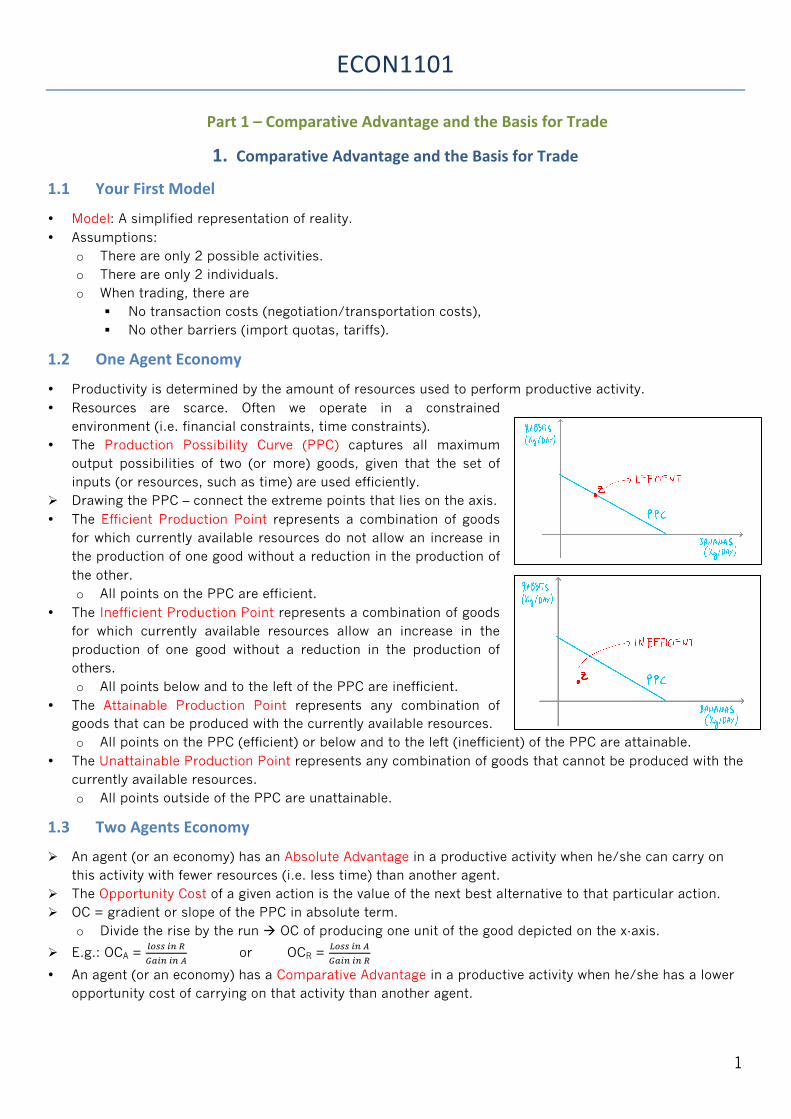
• Productivity can be tabulated as below:

• The Marginal Benefit of producing a certain unit of a given good is the extra benefit accrued by producing

that unit. • The Marginal Cost of producing a certain unit of a given good is the extra cost of producing that unit.

o Note that the relevant cost is the OC, not the absolute cost of producing the good. • Thinking at the margin: comparing the marginal benefit with the marginal cost. This is used to make one

decision after another. • The marginal time indicate the extra time required to produce an extra unit of the good. • The Cost-Benefit Principle states that an action should be taken if the marginal benefit is greater than the

marginal cost. o Marginal benefit ≥ Marginal cost à Take the action. o Marginal benefit < Marginal cost à Don’t take the action.

• The Economic Surplus of a certain action is the difference between the marginal benefit and the marginal cost of taking that action.

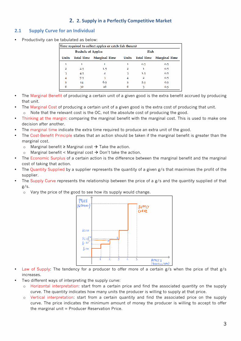
• The Quantity Supplied by a supplier represents the quantity of a given g/s that maximises the profit of the supplier.

• The Supply Curve represents the relationship between the price of a g/s and the quantity supplied of that g/s. o Vary the price of the good to see how its supply would change.

• Law of Supply: The tendency for a producer to offer more of a certain g/s when the price of that g/s

increases. • Two different ways of interpreting the supply curve:

o Horizontal interpretation: start from a certain price and find the associated quantity on the supply curve. The quantity indicates how many units the producer is willing to supply at that price.

o Vertical interpretation: start from a certain quantity and find the associated price on the supply curve. The price indicates the minimum amount of money the producer is willing to accept to offer the marginal unit = Producer Reservation Price.

4

• Producer Reservation Price denotes the minimum amount of money the producer is willing to accept to offer a certain g/s. o E.g.: the producer reservation price for 2 apples is $1.50

2.2 HowtoDerivetheSupplyCurveforaFirm

• A Sunk Cost is a cost that once paid cannot be recovered. E.g.: if a loan is initiated for machinery, the entrepreneur has to repay the borrowing over time.

• If a factor of production is fixed, then its cost does not vary with the quantity produced. o A Fixed Cost is a cost associated with a fixed factor of production – cost is still incurred even when

the firm shuts down. • If a factor of production is variable, then its cost tends to vary with the quantity produced.

o A Variable Cost is a cost associated with a variable factor of production. E.g. Labor. • The Short Run is a period of time which at least one factor of production is fixed. • The Long Run is a period of time during which all factors of production are variable, i.e. producers can

change factor of production as they please.

• From the table above, note that the fixed cost (FC) is a sunk cost, because the producer still needs to pay

$100 even when the quantity produced is zero.

• To maximise profit, the entrepreneur must think at the margin and figure out the optimal number of

employees. Ø Profit represents the difference between total revenues (TR) and the total cost (TC)

𝜋!"#$%&'(#) = 𝑇𝑅 − 𝑇𝐶

• Total revenue = price x quantity • Total cost = fixed cost + variable cost

Should the entrepreneur hire the first worker? Quantity produced (1st worker): 40 cans ($1.20 per can) Fixed cost: $100 (loan) Variable cost: $12 (wage of 1st worker)

Marginal cost (MC) : ∆ !"#$% !"#$∆ !"#$%&%'

= 12/40 = 0.30 ($/unit)

Marginal benefit (MB): Price = 1.20 ($/unit) Because marginal revenue > marginal cost, the first worker should be hired. Continuing this decision-making process concludes that optimal number of employees is four.

Quantity produced (4 workers): 130 cans ($1.20/can) Fixed cost: $100 (loan) Variable cost $48 (wage of 4 workers) Total revenue (4 workers) = Price x Quantity = 130 x 1.20 = $156 Total cost: Fixed Cost + Variable Cost = $100 + $48 = $148

𝜋!"#$%&'!"# = 𝑇𝑅 − 𝑇𝐶= 156 – 148 = $8

5

Ø Shut Down Condition (Short Run): In the short run, the entrepreneur should shut down production if 𝜋!"#$%&'(#) < FC. Otherwise, she should hire the optimal number of workers and continue operations.

Ø Shut Down Condition (Long Run): In the long run, the entrepreneur should exit the industry if

𝜋!"#$%&'(#) < 0. Otherwise, she should hire the optimal number of workers and continue operations.

• In the long run, by exiting the industry the entrepreneur gains and loses nothing because there is no fixed cost (𝜋!"#$ = 0). o This means that entrepreneurs should produce only if the largest profit achievable by doing so is

positive. • If 𝜋!"#$%&'(#) = 0 the entrepreneur is indifferent between exiting and continuing operations.

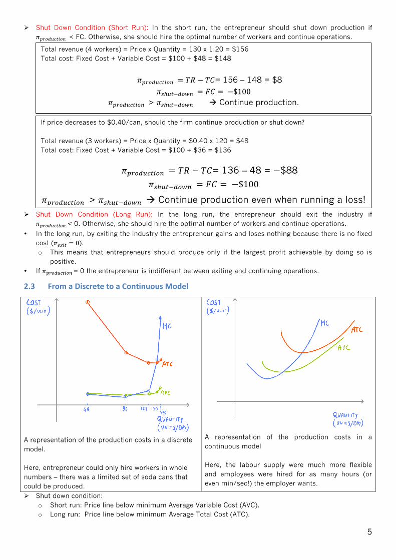
2.3 FromaDiscretetoaContinuousModel

A representation of the production costs in a discrete model. Here, entrepreneur could only hire workers in whole numbers – there was a limited set of soda cans that could be produced.

A representation of the production costs in a continuous model Here, the labour supply were much more flexible and employees were hired for as many hours (or even min/sec!) the employer wants.

Ø Shut down condition: o Short run: Price line below minimum Average Variable Cost (AVC). o Long run: Price line below minimum Average Total Cost (ATC).

Total revenue (4 workers) = Price x Quantity = 130 x 1.20 = $156 Total cost: Fixed Cost + Variable Cost = $100 + $48 = $148

𝜋!"#$%&'(#) = 𝑇𝑅 − 𝑇𝐶= 156 – 148 = $8

𝜋!!!"!!"#$ = 𝐹𝐶 = −$100 𝜋!"#$%&'(#) > 𝜋!!!"!!"#$ à Continue production.

If price decreases to $0.40/can, should the firm continue production or shut down? Total revenue (3 workers) = Price x Quantity = $0.40 x 120 = $48 Total cost: Fixed Cost + Variable Cost = $100 + $36 = $136

𝜋!"#$%&'(#) = 𝑇𝑅 − 𝑇𝐶= 136 – 48 = −$88

𝜋!!!"!!"#$ = 𝐹𝐶 = −$100

𝜋!"#$%&'(#) > 𝜋!!!"!!"#$ à Continue production even when running a loss!

𝜋!"#$%&'(#) > 𝜋!!!"!!"#$ à Continue production.