[1]
EMPIRICALLY-CONSTRAINED CLIMATE
SENSITIVITY AND THE SOCIAL COST OF CARBON
Kevin Dayaratna Heritage Foundation
Washington DC
Ross McKitrick Department of Economics, University of Guelph
and Fraser Institute, Vancouver BC
David Kreutzer US Environmental Protection Agency
Washington DC
February 27, 2017
Forthcoming in Climate Change Economics
Abstract: Integrated Assessment Models (IAMs) require parameterization of both economic and climatic processes. The latter includes Equilibrium Climate Sensitivity (ECS), or the temperature response to doubling CO2 levels, and Ocean Heat Uptake (OHU) efficiency. ECS distributions in IAMs have been drawn from climate model runs that lack an empirical basis, and in Monte Carlo experiments may not be constrained to consistent OHU values. Empirical ECS estimates are now available, but have not yet been applied in IAMs. We incorporate a new estimate of the ECS distribution conditioned on observed OHU efficiency into two widely-used IAMs. The resulting Social Cost of Carbon (SCC) estimates are much lower than those from models based on simulated ECS parameters. In the DICE model the average SCC falls by approximately 40-50% depending on the discount rate, while in the FUND model the average SCC falls by over 80%. The span of estimates across discount rates also shrinks substantially.
Keywords: Social Cost of Carbon; Climate Sensitivity; Ocean Heat Uptake; Carbon Taxes; Integrated Assessment Models Acknowledgments: We thank Nicholas Lewis for comments on an earlier draft. The views expressed in the paper are the authors’ own and do not necessarily represent those of any supporting organizations.

[2]
1 INTRODUCTION Integrated Assessment Models (IAMs) emerged in the 1990s and have become central to the
analysis of global climate policy, especially for estimating the social cost of carbon (SCC)1 or the
marginal damages of an additional unit of carbon dioxide (CO2) emissions. A particularly influential
application has been through the US InterAgency Working Group (IWG 2010, 2013) which estimated
SCC rates for use in US climate and energy regulations. IAMs operate at a high level of abstraction and
require extensive parameterization of both climatic and economic processes. Among the economic
parameters, the most influential are the discount rate and the coefficients of the damages function
(Marten 2011). A key climate parameter is equilibrium climate sensitivity (ECS), which represents
the long term temperature change from doubling atmospheric CO2, after allowing sufficient time for
the deep ocean to respond to surface warming. It is either included explicitly or implicitly in the IAM
functions determining temperature responses to CO2 accumulation.
Optimal SCC estimates depend strongly on the damage function, which in turn is strongly
influenced by ECS (e.g. Webster et al 2008, Ackerman et al. 2010, Wouter Botzen and van den Bergh
2012). ECS uncertainty has multiple dimensions, beginning with the wide range of point estimates
1 Various reviews of IAMs exist, each highlighting or criticizing different aspects, such as Parson and Fisher-
Vanden (1997), Stanton et al. (2009) and Pindyck (2013).
[3]
within the major IAMs (van Vuuren et al. 2011). The interaction between ECS and ocean heat uptake
(OHU) efficiency is an important but largely-overlooked source of uncertainty because it affects the
time-to-equilibrium which affects SCC estimates via the role of discounting (Roe and Bauman 2013;
see below). A number of authors have studied how quickly ECS uncertainty may be reduced over time
via Bayesian learning as new information become available (Kelly and Kolstand 1999, Leach 2007).
Interestingly, Webster et al (2008) find that learning is slowest in the low ECS case while Urban et al.
(2014) find it slowest in the high ECS case, with the difference being due to the role of OHU efficiency.2
IWG (2010, 2013) represented ECS uncertainty by modifying three standard IAMs3 to include a
probability density function (PDF) parameterized to fit a range of estimates from climate modeling
simulations, which then gave rise to a distribution of marginal damages. The choice of ECS
distribution can strongly influence the average SCC if it has a large upper tail, which pulls up both the
median and mean values. The IWG used a PDF from Roe and Baker (2007, herein RB07) which does
have a long upper tail. RB07 was an exploration of why uncertainties over ECS have not been reduced
despite decades of effort, with the explanation centering on the amplified effect of uncertainties in
2 The representation of uncertainty itself can introduce uncertainty. Crost and Traeger (2013) argue that
averaging Monte Carlo runs of deterministic models rather than using a stochastic dynamic programming
(SDP) framework yields inaccurate and potentially incoherent results. But Traeger (2014) finds that applying
SDP in the DICE framework causes problems of dimensionality which necessitate introducing new
simplifications elsewhere, including in the representation of OHU efficiency.
3 The three IAMs are called DICE (Nordhaus 1993), FUND (Tol 1997) and PAGE (Hope 2006).
[4]
the value of the climate feedback parameter f on final temperatures, due to its position in the
denominator of the equation for ECS. To illustrate the point they fitted a curve to a small selection of
ECS estimates published between 2003 and 2007, yielding an ECS curve that had a long upper tail
even though there was no unbounded source of uncertainty in the underlying model.
The reliance by IWG on RB07 is questionable for two reasons. First, as Roe and Bauman (2013)
pointed out, the distribution in RB07 was not directly applicable in the context of IAM simulations
because the wideness of the tails is a function of the time span to equilibrium, which depends heavily
on the assumed OHU efficiency, and the time span associated with the fat upper tail is not relevant to
SCC calculations. In the real world, CO2 doubling is not instantaneous, the transition to a new
equilibrium state is exceedingly slow, and the oceans absorb huge amounts of heat along the way
depending on OHU efficiency. In simplified climate models, time-to-equilibrium increases with the
square of ECS, so an upward adjustment of the ECS parameter outside the range consistent with the
assumed OHU efficiency parameter can yield distorted present value damage estimates. In particular,
the higher the ECS, the slower the adjustment process, making the fat upper tail of realized warming
physically impossible for even a thousand years into the future (Roe and Bauman 2013, p. 653). An
ECS distribution applicable to the real world must therefore be conditioned on a realistic OHU
efficiency estimate.
Second, RB07 predated a large literature on empirical ECS estimation. As was common at the
time, they fitted a distribution to a small number of simulated ECS distributions derived from climate
models. It is only relatively recently that sufficiently long and detailed observational data sets have
been produced to allow direct estimation of ECS using empirical energy balance models. A large
number of studies have appeared since 2010 estimating ECS on long term climatic data (Otto et al.
[5]
2013, Ring et al. 2012, Aldrin et al. 2012, Lewis 2013, Lewis & Curry 2015, Schwartz 2012, Skeie et
al 2014, Lewis 2016, etc.). This literature has consistently yielded median ECS values near or even
below the low end of the range taken from climate model studies. General circulation models (GCMs)
historically yielded sensitivities in the range of 2.0 – 4.5 oC, and (based largely on GCMs) RB07 yields
a central 90 percent range of 1.72 – 7.14 oC with a median of 3.0 oC and a mean of 3.5 oC (see
comparison table in IWG 2010, p. 13). But the median of recent empirical estimates has generally
been between 1.5 and 2.0 oC, with 95% uncertainty bounds below the RB07 average.
This inconsistency has attracted growing attention in the climatology literature (Kummer and
Kessler 2014, Marvel et al. 2015). It is also discussed in the documentation for Nordhaus’ DICE model4
where it is cited as a reason for a slight downward revision in the ECS parameter. However, that
change was based on early evidence published prior to 2008, whereas all the studies discussed herein
were published after 2010.
For the most part, however, the inconsistency between empirical and model-simulated ECS
estimates has been ignored in the climate economics literature. But, as we will show herein, it has
potentially massive policy implications. We replicate the IWG’s SCC estimates using the EPA’s
modified versions of two IAMs (FUND and DICE), 5 then we re-do the calculations using an
observational ECS distribution from a recent study (Lewis and Curry 2015, herein LC15) that controls
for observed OHU efficiency, thereby yielding an empirically-constrained climate sensitivity
4 See http://aida.wss.yale.edu/~nordhaus/homepage/documents/DICE_Manual_100413r1.pdf pp. 17-18.
5 We did not use a third model, PAGE, because its code is unavailable for independent usage.
[6]
distribution. The resulting SCC values drop dramatically compared to those reported in the IWG
(2010, 2013). Using DICE with the model-based RB07 ECS distribution at a 3 percent discount rate
yields a mean SCC for the year 2020 of $37.79, in line with the IWG estimates that currently guide US
policymaking. Substituting the empirical ECS distribution from LC15 yields a mean 2020 SCC of
$19.66, a drop of 48%. The same exercise using FUND yields a mean SCC estimate of $19.33 based
on RB07 and $3.33 based on the LC15 parameters—an 83% decline. Furthermore the probability of
a negative SCC (implying CO2 emissions are a positive externality) jumps dramatically using an
empirical ECS distribution. Using the FUND model, which allows for productivity gains in agricultural
and forestry from higher temperatures and elevated CO2, under the RB07 parameterization at a 3%
discount rate there is only about a ten percent chance of a negative SCC through 2050, but using the
LC15 distribution, the probability of a negative SCC jumps to about 40%. Remarkably, in the FUND
model, replacing simulated climate sensitivity values with an empirical distribution calls into
question whether CO2 is even a negative externality. The lower SCC values also cluster more closely
together across different discount rates, diminishing the importance of this parameter.
We chose the LC15 distribution of ECS because of its explicit treatment of OHU efficiency. The
higher OHU efficiency is, and thus the larger the amount of heat sequestered in the oceans over the
past century, the more the historical climate record understates the total amount of warming that
will ultimately occur (Roe and Bauman 2013). Consequently, estimates of ECS for use in real-world
policy simulations need to take into account information on OHU efficiency as well as CO2 forcing and
temperature records. This is the approach taken in LC15. They used the 1750-2011 forcing and OHU
estimates from the then-most recent IPCC report (IPCC 2014), yielding a median ECS of 1.64 oC and
a 5—95 % uncertainty range of 1.05 – 4.05 oC. This is in line with empirical estimates from Otto et al.
[7]
(2013), Ring et al. (2012), Aldrin et al. (2012) and Lewis (2013), but is in clear contrast to the IWG
parameterization using RB07. The central value in LC15 falls below the 5% lower bound of the ECS
distribution used in IWG (2010, 2013). Not surprisingly, this implies that the corresponding SCC
estimates form a lower and tighter distribution.6
2 SCC CALCULATIONS USING EMPIRICAL PARAMETERS We obtained the code for DICE and FUND7 as used for the IWG (2010, 2013) studies from the US
Environmental Protection Agency. We first replicated the SCC estimates that would have been used
in IWG (2013) from both the DICE and FUND models based on the RB07 ECS distribution. The damage
paths are contingent on the emissions scenarios so five scenarios are used and the results are
averaged.8 As we did not include the PAGE model in our work (due to the unavailability of the code)
6 The distinction is not strictly between empirical and model-simulated estimates. The RB07 distribution
is derived from a simple feedback model fitted to model-derived ECS distributions and so is reasonably labeled
‘simulated’. But the LC15 estimate relies on observational as well as some model-generated data, since forcing
series are not directly observable and must be simulated. For simplicity however we refer to it as an empirical
estimate since it is based on and constrained by observations as much as is feasible.
7 Model authors’ source code is available at http://www.econ.yale.edu/~nordhaus/homepage/ (DICE)
and http://www.fund-model.org/ (FUND). We are grateful to the EPA for providing us with the MATLAB code
they used which contains the modifications for the IWG analysis.
8 The scenarios are called Image, Merge Optimistic, Message, MiniCAM, and 5th Scenario. Four of the five
are business-as-usual scenarios ending in CO2 concentrations between 612 and 889 parts per million. The fifth
[8]
we cannot directly compare our results with the IWG tables since they are averaged over all three
models. IWG (2013) Table A5 lists separate results for FUND and DICE for 2020 and we were able to
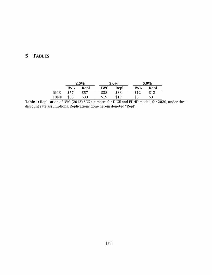
check our results against those. Table 1 shows the DICE and FUND SCC estimates for 2020 compared
with our replications (“Repl”) for three discount rates, demonstrating that we have statistically
reproduced the IWG results.
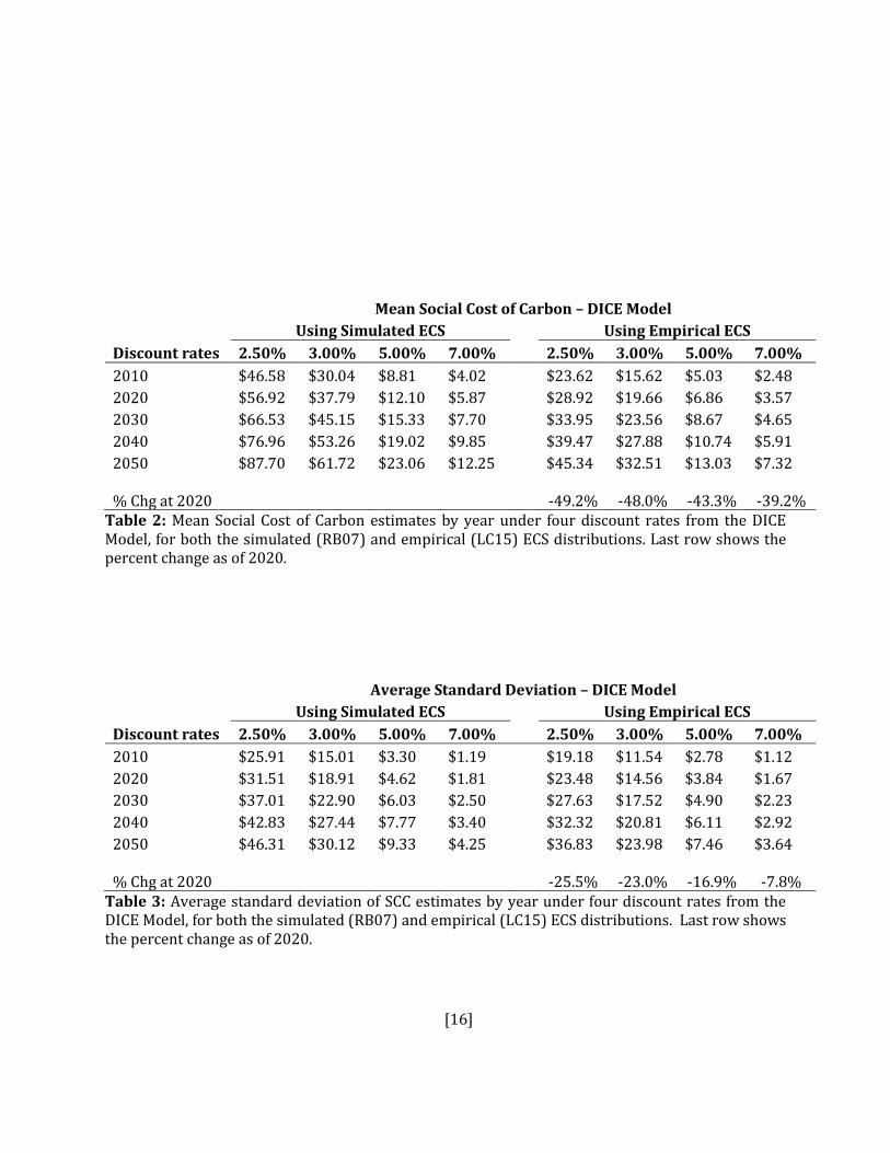
2.1 DICE MODEL Table 2 shows the mean SCC estimates for four discount rates, applying the RB07 and LC15 ECS
distribution to the DICE model. The final row shows the percentage change for the 2020 estimates
(all years exhibit about the same percentage changes). Under the widely-used RB07 distribution, the
SCC ranges from $4.02 to $87.70 depending on the discount rate and the future year. Under the LC15
parameter distributions the SCC ranges from $2.48 to $45.34. For the year 2020 the largest
proportional drop—nearly 50 percent—is observed in the low discount rate case. The high discount
rate case yields a drop of just under 40 percent.
These reductions are primarily due to the LC15 distribution containing a smaller upper tail and
therefore greater probability mass at lower temperatures. Table 3 shows the average standard
deviations of the two sets of estimates. The largest reduction, slightly over 25 percent, again occurs
at the lowest discount rate, compared to only seven percent at the highest discount rate. The LC15
is based either on an assumption of aggressive policy measures or more optimistic assumptions about
technological change that yield an ending concentration of 550 parts per million. See
http://sites.nationalacademies.org/cs/groups/dbassesite/documents/webpage/dbasse_169500.pdf p. 8.

[9]
distribution provides uniformly more certainty for the SCC for all years and all discount rates. These
results are in line with previous research performing similar computations by applying the Otto et al
(2013) ECS distribution in the DICE model (Dayaratna and Kreutzer 2013).
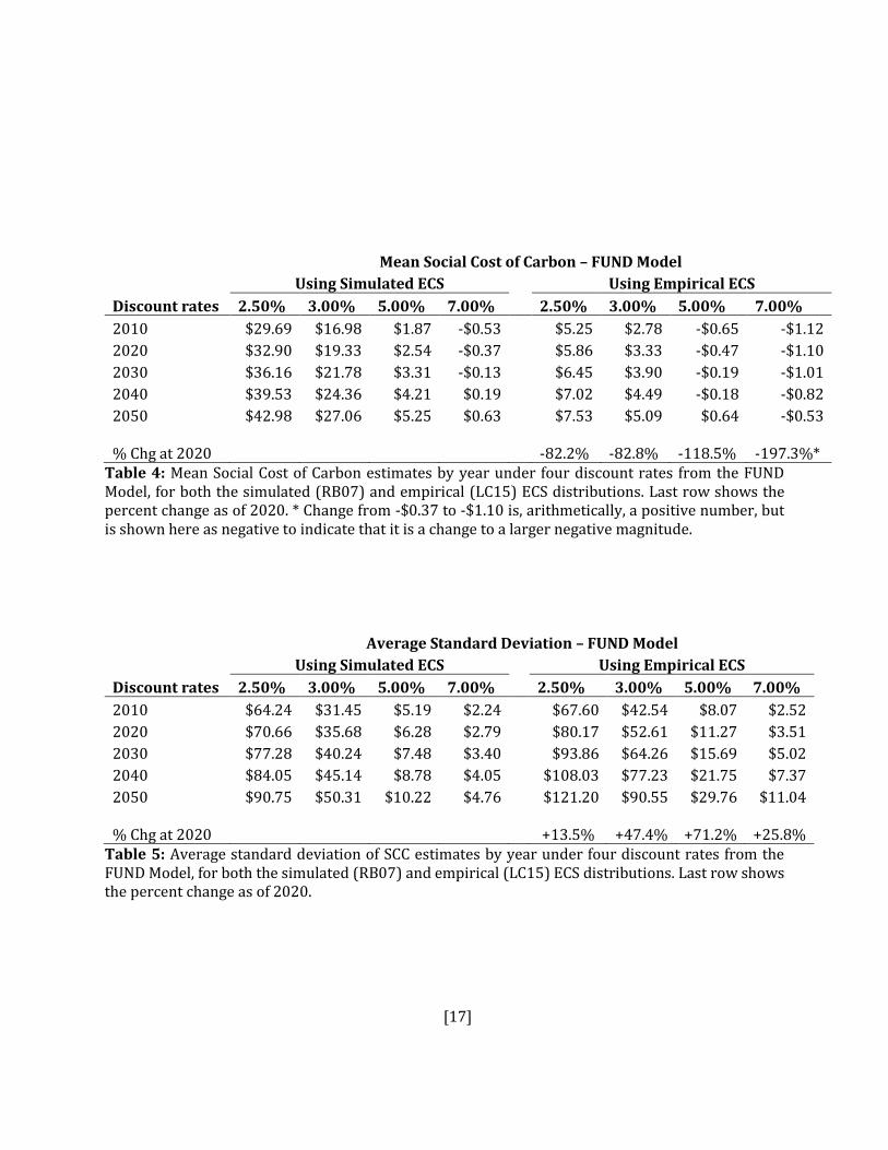
2.2 FUND MODEL Tables 4 and 5 present the same results as Tables 2 and 3, but for the FUND model. A number of
differences are notable. The mean SCC estimates are lower under both parameterizations, and under
the empirical LC15 coefficients they are, on average, mostly negative at 5 percent or higher discount
rates out past 2030. A negative value implies that carbon dioxide emissions are a positive externality,
so that an optimal policy would require subsidizing emissions. Also, in contrast to the DICE model,
use of the LC15 coefficients increases the average standard deviation, indicating higher uncertainty
compared to the RB case.9 The increased uncertainty includes a much larger lower tail, implying a
larger probability of a negative SCC. DICE is constrained to a transformed quadratic global damage
function such that damages cannot be negative regardless of temperature change. FUND allows the
gains for regions that benefit from moderate warming to potentially outweigh the costs in other
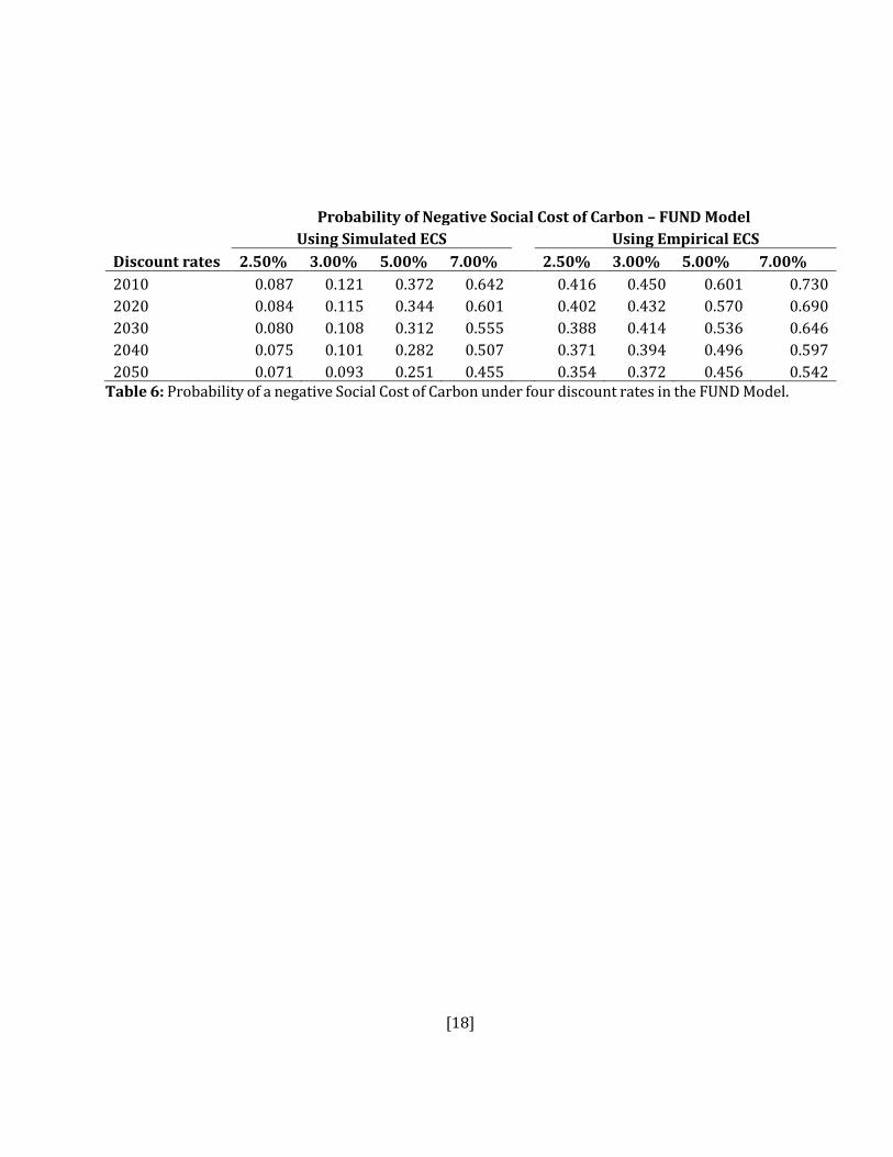
regions so some scenarios can yield negative net costs at the global level. Table 6 shows that, under
the RB07 parameterization, at a 2.5 percent discount rate the probability of carbon dioxide emissions
9 ECS is the only stochastic parameter in DICE so the reduction in variance between RB07 and LC15 leads
automatically to a corresponding reduction in the SCC variance. By contrast, dozens of parameters in FUND are
stochastic so reduction in the mean and variance of ECS interacts in a more complex way with the rest of the
model. The net effect, as shown is to increase the spread of SCC estimates.
[10]
being a positive externality is only 7.1 percent in 2050. But using the LC15 parameters this
probability jumps to over 35 percent.
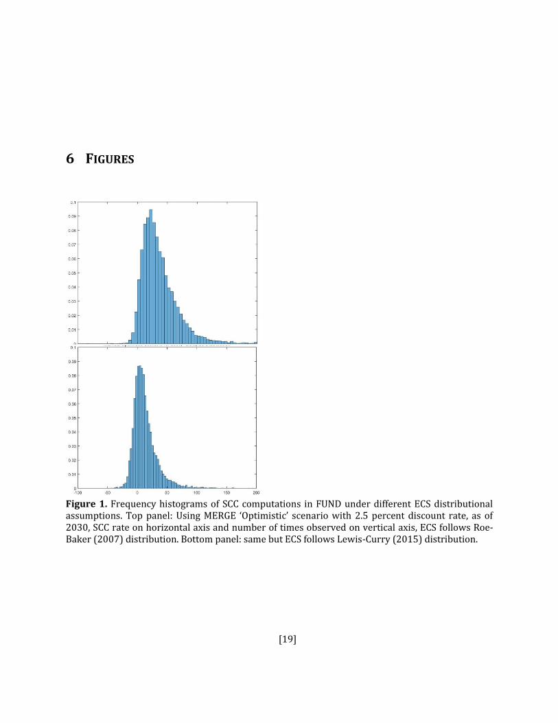
Figure 1 shows normalized histograms of SCC calculations for the Merge Optimistic scenario at
2.5 percent discounting as of 2030. The height of each bar represents the probability of choosing an
observation within a particular bin interval, and the sum of the heights across all of the bars is equal
to 1. The bin width for RB07 is 5, the bin width of LC15 is 3. Comparing the top and bottom panels
we see that model simulation of ECS introduces uncertainty not found in observations by creating an
extended upper tail.
These results are in line with previous simulations using other ECS distributions that have
smaller upper tails than RB07, namely Otto et al (2013) and Lewis (2013); see Dayaratna and
Kreutzer (2014). Figure 2 summarizes the calculations by comparing the mean of DICE- and FUND-
computed SCC values from 2010 to 2050 at a 3 percent discount rate using the simulated (black,
upper line) and the empirical (gray, lower line) ECS values. As of 2050 the empirically-constrained
value ($18.80) is still below the 2010 value ($23.51) based on simulated ECS.
3 DISCUSSION AND CONCLUSION IAMs play an important role in climate policy analysis. They rely on a number of influential
parameter choices, such as ECS. Model-based ECS distributions are misleading for use in SCC
calculations because they are not conditioned on OHU efficiency rates relevant to IAM timelines and
because they are skewed high relative to the current empirical evidence. The model-observational
discrepancy in ECS estimation is not attributable simply to a specific empirical methodology, as
similar results have been found by Otto et al. (2013), Ring et al. (2012), Aldrin et al. (2012) and others
[11]
using a variety of methods. Nor is it an artifact of selecting a specific estimation period, as LC15
showed their results were robust to numerous variations on the choice of base and final periods
(LC15, Table 4).
We incorporated the Lewis and Curry (2015) ECS distribution, which is conditioned on updated
forcings and OHU data, into the DICE and FUND models. This reduces the estimated Social Cost of
Carbon in both, regardless of discount rates. Using a 3 percent discount rate and the RB07 ECS
distribution, DICE yields an average SCC ranging from about $30 to $60 between now and 2050, but
this falls to the $15 to $33 range using the LC15 ECS estimate. The corresponding average SCC in
FUND falls from the $17 to $27 range to the $3 to $5 range. Moreover FUND, which takes more explicit
account of potential regional benefits from CO2 fertilization and increased agricultural productivity,
yields a substantial (about 40 percent) probability of a negative SCC through the first half of the 21st
century, putting into question whether CO2 is even a net social cost or benefit.
A further way in which use of empirically-constrained parameters reduces uncertainty is the
shrinking of the SCC range across discount rates. In the DICE model under the RB07
parameterization, the mean SCC estimates span over $45 as of 2010 depending on choice of discount
rate, with the span rising to over $85 as of 2050. This span shrinks to the $23 to $64 range under the
LC15 parameterization. Using the FUND model, the uncertainty range associated with the choice of
discount rate is from about $30 to $43 under the RB07 parameterization, falling to $5 to $8 range
under the LC15 parameterization. Thus, use of well-constrained empirical parameters makes a
substantial contribution also to reducing uncertainty associated with the choice of discount rate.

[12]
4 REFERENCES Ackerman, F., A.A. Stanton and Ramón Bueno (2010) Fat tails, exponents, extreme uncertainty:
Simulating catastrophe in DICE. Ecological Economics 69 (2010) 1657–1665. Aldrin, M., M. Holden, P. Guttorp, R. B. Skeie, G. Myhre, and T. K. Berntsen, (2012): Bayesian estimation
of climate sensitivity based on a simple climate model fitted to observations of hemispheric temperatures and global ocean heat content. Environmetrics, 23, 253-271.
Crost, B. and C. P. Traeger (2013) Optimal Climate Policy: Uncertainty versus Monte Carlo Economics Letters 120: 552-558.
Dayaratna, Kevin and David Kreutzer (2013) Loaded DICE: An EPA Model Not Ready for the Big Game. Heritage Foundation Center for Data Analysis Backgrounder No. 2860, Washington DC, November 21, 2013. http://report.heritage.org/bg2860
Dayaratna, Kevin and David Kreutzer (2014) Unfounded FUND: Another EPA Model Not Ready for the Big Game. Heritage Foundation Center for Data Analysis Backgrounder No. 2897, Washington DC, April 29, 2014. http://report.heritage.org/bg2897
Hansen J et al. (2005) Efficacy of climate forcings. Journal of Geophysical Research 110:D18104. doi:10.1029/2005JD005776
Hope C. (2006) The marginal impact of CO2 from PAGE2002: an integrated assessment model incorporating the IPCC’s five reasons for concern. The Integrated Assessment Journal 6(1):19-56.
Intergovernmental Panel on Climate Change (IPCC) (2007) Climate Change 2007: The Physical Science Basis. Working Group I Contribution to the Fourth Assessment Report of the IPCC. Cambridge: Cambridge University Press.
Kelly, D. L., and C. D. Kolstad. (1999) Bayesian learning, growth, and pollution. Journal of Economic Dynamics and Control 23, no. 4: 491-518
Kiehl, J.T. (2007) “Twentieth century climate model response and climate sensitivity.” Geophysical Research Letters 34 L22710, doi:10.1029/2007GL031383, 2007.
Kummer, J.R. and A.E. Dessler (2014) “The impact of forcing efficacy on the equilibrium climate sensitivity.” Geophysical Research Letters 10.1002/2014GL060046 .
Leach, A. J. (2007) The climate change learning curve. Journal of Economic Dynamics and Control 31, no. 5: 1728-1752.
Lewis, N. and J.A. Curry, C., (2015). The implications for climate sensitivity of AR5 forcing and heat uptake estimates. Climate Dynamics, 10.1007/s00382-014-2342-y.
Lewis, N., (2013) An objective Bayesian, improved approach for applying optimal fingerprint techniques to estimate climate sensitivity. Journal of Climate, 26, 7414-7429.
Lewis, N., (2016) Implications of recent multimodel attribution studies for climate sensitivity. Climate Dynamics, 46(5), 1387-1396
Marten, Alex L. (2011) “Transient Temperature Response Modeling in IAMs: The Effects of Over Simplification on the SCC.” Economics E-Journal Vol. 5, 2011-18 | October 20, 2011 | http://dx.doi.org/10.5018/economics-ejournal.ja.2011-18.
Marvel, K., G.A. Schmidt, R.L. Miller and L.S. Nazarenko (2015) Implications for climate sensitivity from the response to individual forcings. Nature Climate Change 14 December 2015 DOI: 10.1038/NCLIMATE2888.
Marvel, K., G.A. Schmidt, R.L. Miller and L.S. Nazarenko (2016) Online correction to: Implications for climate sensitivity from the response to individual forcings. Nature Climate Change

[13]
http://www.nature.com/nclimate/journal/vaop/ncurrent/full/nclimate2888.html#correction1 Accessed March 14, 2016.
Nordhaus, W. (1993) Optimal Greenhouse-Gas Reductions and Tax Policy in the "DICE" Model American Economic Review Vol. 83, No. 2, (Papers and Proceedings) pp.313-317.
Nordhaus, W. and P. Sztorc (2013) DICE 2013R: Introduction and User’s Manual. Yale University http://aida.wss.yale.edu/~nordhaus/homepage/documents/DICE_Manual_100413r1.pdf
Otto, A, Otto, FEL, Allen, MR, Boucher, O, Church, J, Hegerl, G, Forster, PM, Gillett, NP, Gregory, J, Johnson, GC, Knutti, R, Lohmann, U, Lewis, N, Marotzke, J, Stevens, B, Myhre, G and Shindell, D (2013) Energy budget constraints on climate response. Nature Geoscience, 6, 415–416.
Parson, Edward A. and Karen Fisher-Vanden (1997) Integrated Assessment Models of Global Climate Change. Annual Review of Energy and the Environment 22:589—628.
Pindyck, Robert S. (2013) Climate Change Policy: What do the Models Tell Us? Journal of Economic Literature 51(3), 860–872 http://dx.doi.org/10.1257/jel.51.3.860.
Ring, M.J., D. Lindner, E.F. Cross and M. E. Schlesinger (2012) Causes of the Global Warming Observed since the 19th Century. Atmospheric and Climate Sciences, 2, 401-415.
Roe, Gerard H. and Marcia B. Baker, (2007) Why Is Climate Sensitivity So Unpredictable? Science, Vol. 318, No. 5850 (October 26, 2007), pp. 629–632.
Roe, Gerard H. and Yoram Bauman (2013) Climate Sensitivity: Should the climate tail wag the policy dog? Climatic Change (2013) 117:647–662 DOI 10.1007/s10584-012-0582-6
Schwartz S.E. (2012) Determination of Earth’s transient and equilibrium climate sensitivities from observations over the twentieth century: strong dependence on assumed forcing. Surveys in Geophysics 33(3–4):745–777.
Schwartz, Stephen E., R.J. Charlson and H. Rodhe (2007) Quantifying climate change—too rosy a picture? Nature reports climate change 2 23—24.
Skeie, R.B., T. Berntsen, M. Aldrin, M. Holden, and G. Myhre. A lower and more constrained estimate of climate sensitivity using updated observations and detailed radiative forcing time series. Earth System Dynamics 5, 139–175, 2014 doi:10.5194/esd-5-139-2014.
Stanton, Elizabeth, Frank Ackerman and Sivan Kartha (2009) Inside the integrated assessment models: Four issues in climate economics, Climate and Development, 1:2, 166-184.
Tol, R.S.J. (1997) On the optimal control of carbon dioxide emissions: an application of FUND Environmental Modeling and Assessment 2: 151—163.
Traeger, C. P. (2014) A 4-Stated DICE: Quantitatively Addressing Uncertainty Effects in Climate Change Environmental and Resource Economics 59:1—37.
Urban, N.M., P.B. Holden, N.R. Edwards, R.L. Sriver and K. Keller (2014) Historical and future learning about climate sensitivity. Geophysical Research Letters 41, 2543–2552, doi:10.1002/2014GL059484.
US Interagency Working Group on Social Cost of Carbon (IWG) (2013) “Technical Support Document: Technical update of the social cost of carbon for regulatory impact analysis Under Executive Order 12866.” United States Government.
US Interagency Working Group on Social Cost of Carbon (IWG) (2010). “Social Cost of Carbon for Regulatory Impact Analysis under Executive Order 12866.” United States Government. http://www.whitehouse.gov/sites/default/files/omb/inforeg/for-agencies/Social-Cost-of-Carbon-for-RIA.pdf.
[14]
van Vuuren, D., Lowe, J., Stehfest, E., Gohar, L., Hof, A., Hope, C., Warren, R., Meinshausen, M., and Plattner, G. (2011) How well do integrated assessment models simulate climate change? Climatic Change, 104(2): 255–285.
Webster, Mort, Lisa Jakobovits and James Norton 2008 Learning about climate change and implications for near-term policy. Climatic Change 89:67–85 DOI 10.1007/s10584-008-9406-0
Wouter Botzen, W.J. and J.C.J.M. van den Bergh (2012) How sensitive is Nordhaus to Weitzman? Climate policy in DICE with an alternative damage function. Economics Letters 117: 372—374.
[15]
5 TABLES
2.5% 3.0% 5.0% IWG Repl IWG Repl IWG Repl DICE $57 $57 $38 $38 $12 $12 FUND $33 $33 $19 $19 $3 $3
Table 1: Replication of IWG (2013) SCC estimates for DICE and FUND models for 2020, under three discount rate assumptions. Replications done herein denoted “Repl”.
[16]
Mean Social Cost of Carbon – DICE Model
Using Simulated ECS Using Empirical ECS
Discount rates 2.50% 3.00% 5.00% 7.00% 2.50% 3.00% 5.00% 7.00%
2010 $46.58 $30.04 $8.81 $4.02 $23.62 $15.62 $5.03 $2.48
2020 $56.92 $37.79 $12.10 $5.87 $28.92 $19.66 $6.86 $3.57
2030 $66.53 $45.15 $15.33 $7.70 $33.95 $23.56 $8.67 $4.65
2040 $76.96 $53.26 $19.02 $9.85 $39.47 $27.88 $10.74 $5.91
2050 $87.70 $61.72 $23.06 $12.25 $45.34 $32.51 $13.03 $7.32 % Chg at 2020 -49.2% -48.0% -43.3% -39.2%
Table 2: Mean Social Cost of Carbon estimates by year under four discount rates from the DICE Model, for both the simulated (RB07) and empirical (LC15) ECS distributions. Last row shows the percent change as of 2020.
Average Standard Deviation – DICE Model
Using Simulated ECS Using Empirical ECS
Discount rates 2.50% 3.00% 5.00% 7.00% 2.50% 3.00% 5.00% 7.00%
2010 $25.91 $15.01 $3.30 $1.19 $19.18 $11.54 $2.78 $1.12
2020 $31.51 $18.91 $4.62 $1.81 $23.48 $14.56 $3.84 $1.67
2030 $37.01 $22.90 $6.03 $2.50 $27.63 $17.52 $4.90 $2.23
2040 $42.83 $27.44 $7.77 $3.40 $32.32 $20.81 $6.11 $2.92
2050 $46.31 $30.12 $9.33 $4.25 $36.83 $23.98 $7.46 $3.64 % Chg at 2020 -25.5% -23.0% -16.9% -7.8%
Table 3: Average standard deviation of SCC estimates by year under four discount rates from the DICE Model, for both the simulated (RB07) and empirical (LC15) ECS distributions. Last row shows the percent change as of 2020.
[17]
Mean Social Cost of Carbon – FUND Model
Using Simulated ECS Using Empirical ECS
Discount rates 2.50% 3.00% 5.00% 7.00% 2.50% 3.00% 5.00% 7.00%
2010 $29.69 $16.98 $1.87 -$0.53 $5.25 $2.78 -$0.65 -$1.12
2020 $32.90 $19.33 $2.54 -$0.37 $5.86 $3.33 -$0.47 -$1.10
2030 $36.16 $21.78 $3.31 -$0.13 $6.45 $3.90 -$0.19 -$1.01
2040 $39.53 $24.36 $4.21 $0.19 $7.02 $4.49 -$0.18 -$0.82
2050 $42.98 $27.06 $5.25 $0.63 $7.53 $5.09 $0.64 -$0.53 % Chg at 2020
-82.2% -82.8% -118.5% -197.3%*
Table 4: Mean Social Cost of Carbon estimates by year under four discount rates from the FUND Model, for both the simulated (RB07) and empirical (LC15) ECS distributions. Last row shows the percent change as of 2020. * Change from -$0.37 to -$1.10 is, arithmetically, a positive number, but is shown here as negative to indicate that it is a change to a larger negative magnitude.
Average Standard Deviation – FUND Model
Using Simulated ECS Using Empirical ECS
Discount rates 2.50% 3.00% 5.00% 7.00% 2.50% 3.00% 5.00% 7.00%
2010 $64.24 $31.45 $5.19 $2.24 $67.60 $42.54 $8.07 $2.52
2020 $70.66 $35.68 $6.28 $2.79 $80.17 $52.61 $11.27 $3.51
2030 $77.28 $40.24 $7.48 $3.40 $93.86 $64.26 $15.69 $5.02
2040 $84.05 $45.14 $8.78 $4.05 $108.03 $77.23 $21.75 $7.37
2050 $90.75 $50.31 $10.22 $4.76 $121.20 $90.55 $29.76 $11.04 % Chg at 2020
+13.5% +47.4% +71.2% +25.8%
Table 5: Average standard deviation of SCC estimates by year under four discount rates from the FUND Model, for both the simulated (RB07) and empirical (LC15) ECS distributions. Last row shows the percent change as of 2020.
[18]
Probability of Negative Social Cost of Carbon – FUND Model
Using Simulated ECS Using Empirical ECS
Discount rates 2.50% 3.00% 5.00% 7.00% 2.50% 3.00% 5.00% 7.00%
2010 0.087 0.121 0.372 0.642 0.416 0.450 0.601 0.730
2020 0.084 0.115 0.344 0.601 0.402 0.432 0.570 0.690
2030 0.080 0.108 0.312 0.555 0.388 0.414 0.536 0.646
2040 0.075 0.101 0.282 0.507 0.371 0.394 0.496 0.597
2050 0.071 0.093 0.251 0.455 0.354 0.372 0.456 0.542 Table 6: Probability of a negative Social Cost of Carbon under four discount rates in the FUND Model.
[19]
6 FIGURES
Figure 1. Frequency histograms of SCC computations in FUND under different ECS distributional assumptions. Top panel: Using MERGE ‘Optimistic’ scenario with 2.5 percent discount rate, as of 2030, SCC rate on horizontal axis and number of times observed on vertical axis, ECS follows Roe-Baker (2007) distribution. Bottom panel: same but ECS follows Lewis-Curry (2015) distribution.

[20]
Figure 2. Social Cost of Carbon Estimates, 2010 – 2050, average of DICE and FUND models applying a 3 percent discount rate. Top (black) line using simulated ECS parameter distribution. Bottom (gray) line using empirical ECS parameter distribution.
$0
$5
$10
$15
$20
$25
$30
$35
$40
$45
$50
2000 2010 2020 2030 2040 2050 2060
Simulated ECS (RB07)
Empirical ECS (LC15)
Recommended