EXPERIMENTAL INVESTIGATION OF ENHANCED COAL BED
METHANE RECOVERY
A REPORT SUBMITTED TO THE DEPARTMENT OF PETROLEUM ENGINEERING
OF STANFORD UNIVERSITY
IN PARTIAL FULFILLMENT OF THE REQUIREMENTS FOR THE DEGREE OF MASTER OF SCIENCE
By Sameer Parakh
July 2007


iii
I certify that I have read this report and that in my opinion it is fully adequate, in scope and in quality, as partial fulfillment of the degree of Master of Science in Petroleum Engineering.
__________________________________
Prof. Margot Gerritsen (Principal Advisor)


v
Abstract
Enhanced coal bed methane recovery involves simultaneous adsorption-desorption,
diffusion and convection phenomena in the coal beds which can structurally be divided
into matrix and cleats. This complex mechanism in a one-dimensional system is
described by a non-linear, hyperbolic differential equation. Extensive work has been
performed to solve the system analytically by method of characteristics. Solutions for
binary, ternary and quaternary mixtures consisting of single and two-phase systems show
the effects of component adsorption, volatility and injection gas composition on the
solution profiles.
This thesis presents a systematic approach of conducting experiments for performing one-
dimensional slim tube displacement for enhanced coal bed methane recovery. The
purposes of the experimental studies are to understand the reservoir mechanisms of CO2
and N2 injection into coal beds, demonstrate the practical effectiveness of the ECBM and
sequestration processes and the engineering capability to simulate them, and to validate
the analytical results and conclusions.
Single phase experiments are first conducted to investigate methane recovery by injection
of pure and mixed gases. A tracer test is then conducted with non-adsorbing gases to find
the dispersion coefficient of gases in coal tube. The result is useful to perform numerical
simulations for the single phase systems. Two-phase investigations are further performed
to validate the analytical results for different injection gas compositions.
The experimental results are in good agreement with the analytical solutions. The
calculation of dispersion coefficient is validated by both experimental and theoretical
models and its application in the numerical simulation drives the spatially and temporally
refined solutions to match with the dispersed experimental results. Two-phase

vi
experiments confirm the analytical theory for saturated and under-saturated systems and
also show the presence of a degenerate shock in the solution profile for mixture injection.

vii
Acknowledgments
I am highly indebted to my advisors Prof. Lynn Orr and Prof. Margot Gerritsen for their
role as an excellent guide during my graduate studies at Stanford University. The unique
experience of working with two experts in the fields of analytical and computational
modeling was highly rewarding during my research work. I would like to thank them for
their encouragement and patience shown to me for doing challenging experiments. I
would also like to thank Prof. Anthony R. Kovscek for helping me design my
experimental setup and for his constant technical support.
I am thankful to Dr. Tom Tang, Dr. Louis Castanier, and Aldo Rossi for helping me build
my experimental setup. I would also like to acknowledge the support of Mohamed
Hassam from CMG for helping me build the simulation model.
I would like to thank the SUPRI-C group for financially supporting my graduate study
and research. A special thanks to all the colleagues in the department for making my stay
at Stanford a memorable one.
Finally, I would like to thank my grandparents, my parents and my sisters who have been
a constant source of inspiration for me.


ix
Table of Contents
Abstract……………………………………………………………………………………v
Acknowledgments............................................................................................................. vii
Table of Contents............................................................................................................... ix
List of Tables ..................................................................................................................... xi
List of Figures ..................................................................................................................xiii
1. Introduction................................................................................................................. 1
1.1. Current usage and energy recovery statistics of coal .......................................... 2 1.2. Technology in energy recovery from coal: Enhanced Coal Bed Methane
Recovery ............................................................................................................. 4 1.3. CO2 sequestration and ECBM ............................................................................ 5 1.4. Analytical modeling for enhanced coal bed methane recovery........................... 6
2. Theory of ECBM Recovery ........................................................................................ 9
2.1. Flow characteristics in coal................................................................................. 9 2.2. The physics of coal bed methane recovery ....................................................... 10 2.3. Physics of the enhanced coal bed methane recovery process ........................... 11
3. Experimental Design................................................................................................. 15
3.1. Study of coal characteristics.............................................................................. 15 3.2. Slim tube configuration..................................................................................... 16 3.3. Flow rate determination .................................................................................... 17 3.4. Single phase experiments.................................................................................. 18
3.4.1. Binary displacement.................................................................................. 20 3.4.2. Determination of dispersion coefficient................................................... 20 3.4.3. Ternary displacement with mixture injection ........................................... 21
3.5. Two-phase experiments .................................................................................... 21 3.5.1. Ternary displacement with pure CO2 injection......................................... 23 3.5.2. Quaternary displacement with mixture injection ...................................... 23
3.6. One-dimensional numerical simulation ............................................................ 25 4. Operating Procedure ................................................................................................. 27
5. Results, Discussion and Material Balance ................................................................ 33
5.1. Results for pure CO2 injection for methane displacement................................ 33 5.2. Results for pure N2 injection for methane displacement................................... 37

x
5.3. Results for dispersion experiment..................................................................... 40 5.4. Results for methane displacement by injection of a mixture of N2 and CO2 .... 42 5.5. Comparison of the single phase experiments with different injection gases .... 45 5.6. Results for displacement of water and methane by pure CO2 injection............ 47 5.7. Results for displacement of water and methane by mixture injection .............. 49 5.8. Effects of saturated and under saturated initial conditions and comparison with
analytical solutions............................................................................................ 54 5.9. Numerical study of ECBM recovery................................................................. 56
5.9.1. Simulation of methane displacement by pure CO2 ................................... 58 5.9.2. Simulation of methane displacement by pure N2 ...................................... 59 5.9.3. Simulation of methane displacement by mixture of CO2 and N2 ............. 60
6. Conclusions............................................................................................................... 62
Nomenclature…………………………………………………………………………….65 References………………………………………………………………………………..68 Appendix
A. Individual Components of Experimental Setup................................................ 72 B. Porosity Measurement Data .............................................................................. 77 C. Permeability Measurement Data ....................................................................... 78 D. Simulation Data File ......................................................................................... 79

xi
List of Tables
Table 3-1: Operating conditions for single phase experiments......................................... 21
Table 3-2: Analytical vs realistic K values (Seto, 2007) .................................................. 23
Table 3-3: Operating conditions for two-phase experiments............................................ 25
Table 4-1: Method setup for running sequences in the GC .............................................. 30
Table 5-1: Material balance calculations for pure CO2 injection...................................... 35
Table 5-2: Material balance calculations for N2 injection ................................................ 39
Table 5-3: Material balance calculations for mixture injection in single phase system ... 44
Table 5-4: Material balance calculations for water injection in methane saturated coal .. 51
Table 5-5: Material balance for mixture injection in water + methane saturated coal ..... 53
Table 5-6: Material balance for CO2 capture in saturated and under-saturated systems... 56
Table 5-7: Discretization parameters for dispersion experiment ...................................... 57
Table 5-8: Discretization parameters for pure CO2 injection in methane saturated coal.. 59
Table 5-9: Discretization parameters for pure N2 injection in methane saturated coal .... 59
Table 5-10: Discretization parameters for mixture injection in methane saturated coal .. 60
Table B: Porosity measurement data................................................................................. 77
Table C: Permeability measurement data ......................................................................... 78

xiii
List of Figures
Figure 1-1: Coal resources in the continental United States (Britannica)........................... 2
Figure 1-2: Fractions of methane production from various coal basins in the US (Smith,
2003) ................................................................................................................................... 3
Figure 1-3: Schematic of Enhanced Coal Bed Methane Recovery project (Seto, 2007) .... 4
Figure 2-1: Adsorption-desorption isotherm for gases on coal (Tang. et al. 2005).......... 12
Figure 2-2: Relative permeability curves for gas-water system in coal packing
(Chaturvedi, 2006) ............................................................................................................ 13
Figure 3-1: Powder River Basin coal in raw (a) and crushed (b) forms ........................... 15
Figure 3-2: Coal particles at 20X (a) and 50X (b) magnification ..................................... 16
Figure 3-3: Single particles at 50X magnification ............................................................ 16
Figure 3-4: Effect of injection velocity on residual trapping (Hill, 1949) ........................ 18
Figure 3-5: Analytical results for injection of mixture of CO2 and N2 (50-50) for methane
displacement (Zhu, 2003) ................................................................................................. 19
Figure 3-6: Schematic diagram of experimental setup for the single phase systems........ 19
Figure 3-7: Schematic diagram of the experimental setup for the two phase systems ..... 22
Figure 3-8: Analytical results for injection of mixture of CO2 and N2 (60:40) for two-
phase displacement (Seto, 2007)....................................................................................... 24
Figure 4-1: Gas cylindrical bomb (a) and pressure gauge (b) ........................................... 27
Figure 4-2: Methane injection in coal tube ....................................................................... 29
Figure 5-1: Total production rate for pure CO2 injection. ................................................ 33
Figure 5-2: Composition profile at tube outlet for pure CO2 injection............................. 34
Figure 5-3: Component molar rates for pure CO2 injection.............................................. 35
Figure 5-4: Cumulative moles produced for pure CO2 injection ...................................... 35
Figure 5-5: Fractional molar recovery of methane for pure CO2 injection ....................... 36
Figure 5-6: Comparison of composition profiles of experimental (a) and analytical (b)
solutions for pure CO2 injection ....................................................................................... 36
Figure 5-7: Total production rate for pure N2 injection .................................................... 37

xiv
Figure 5-8: Composition profile at tube outlet for pure N2 injection................................ 38
Figure 5-9: Component molar rates for pure N2 injection ................................................ 38
Figure 5-10: Cumulative moles produced for pure N2 injection....................................... 39
Figure 5-11: Methane recovery for pure N2 injection ....................................................... 39
Figure 5-12: Comparison of composition profiles of experimental (a) and analytical (b)
solutions for pure N2 injection .......................................................................................... 40
Figure 5-13: Helium fraction in the produced gas ............................................................ 40
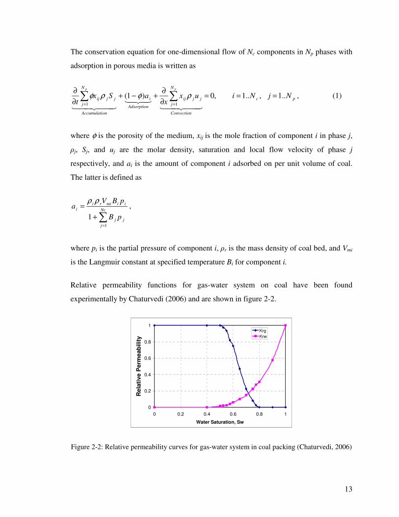
Figure 5-14: Measurement of dispersion coefficient ........................................................ 42
Figure 5-15: Composition profiles for CO2, N2 and methane for mixture injection......... 43
Figure 5-16: Total production rate for mixture injection in single phase system ............. 43
Figure 5-17: Production profiles for mixture injection..................................................... 44
Figure 5-18: Methane recovery for mixture injection in single phase system .................. 44
Figure 5-19: Comparison of composition profiles of experimental (a) and analytical (b)
solutions for mixture injection in single phase systems.................................................... 45
Figure 5-20: Experimental results for Methane recovery by different injection gases ..... 45
Figure 5-21: Experimental results for total production rate with different injection gases
........................................................................................................................................... 46
Figure 5-22: Experimental results for methane production rate by different injection gases
........................................................................................................................................... 47
Figure 5-23: Composition profile for CO2 injection in coal with methane and water
saturation........................................................................................................................... 47
Figure 5-24: Fractional water production for CO2 injection in methane and water
saturated coal .................................................................................................................... 48
Figure 5-25: Comparison of experimental (a) and analytical (b) results for pure CO2
injection in water + methane saturated system ................................................................. 48
Figure 5-26: Injection and production profiles for water injection................................... 49
Figure 5-27: Production profiles for water injection in methane saturated coal............... 50
Figure 5-28: Composition profile of exit gases for mixture injection .............................. 51
Figure 5-29: Injection and production profiles ................................................................. 52
Figure 5-30: Water and methane recovery for mixture injection in two-phase system .... 52

xv
Figure 5-31: Comparison of experimental (a) and analytical (b) results for mixture
injection in water + methane saturated system ................................................................. 54
Figure 5-32: Comparison of experimental (a) and analytical (b) solutions for saturated
and under-saturated systems ............................................................................................. 55
Figure 5-33: Composition profiles of CO2 in saturated and undersaturated systems ....... 56
Figure 5-34: Convergence test for dispersion experiment ................................................ 57
Figure 5-35: Effect of increasing the numerical diffusion ................................................ 57
Figure 5-36: Composition profile for dispersion experiment ........................................... 58
Figure 5-37: Simulation and experimental comparisons for pure CO2 injection.............. 59
Figure 5-38: Simulation and experimental comparisons for pure N2 injection ................ 60
Figure 5-39: Simulation and experimental comparisons for mixture injection ................ 61
Figure A-1: Gas Chromatograph....................................................................................... 74
Figure A-2: Schematic of the valve and column configuration inside the GC ................. 74
Figure A-3: Overall setup for single phase experiments................................................... 75
Figure A: The different pieces of the experimental setup................................................. 76


1
Chapter 1
1. Introduction
In reservoir engineering terms, coal beds are naturally fractured, low-pressure, water-
saturated reservoirs, where most of the gas is retained in the micro-pore structure of the
coal by physical adsorption. A reservoir is that portion of the coal seam that contains gas
and water as a connected system. Thus coal serves as a reservoir and a source rock,
containing relatively pure methane. The mechanisms governed by coupled convective,
adsorptive and dispersive phenomena in coal are currently being studied for enhanced
recovery of methane from coal as well as from CO2 sequestration point of view.
Analytical modeling and numerical simulations have been performed for one-dimensional
transport of single phase (Zhu, 2003) and multi-phase (Seto, 2007) multi-component
mixtures in coal, utilizing the method of characteristics solutions for non-linear
hyperbolic equations, as outlined in Orr (2007). Analytical solutions to convection
dominated displacements provide insight into the interplay of flow, phase behavior and
sorption in ECBM processes. It shows that adsorption of CO2 onto the coal reduces the
propagation velocity of the CO2 front, delaying breakthrough time of CO2 at the
production well thereby allowing for more CO2 to be sequestered per amount of methane
produced. The study also concludes that if pure CO2 is injected, pure methane is produced
until breakthrough of the injected CO2. Displacement of methane by N2 occurs via a
partial pressure reduction. Volume change as methane desorbs results in a faster recovery
of methane, though the produced gas is now a mixture of N2 and methane. Apart from
these analytical models, laboratory experiments have also been performed in a coal pack
for single phase flow studies by Tang, Jessen and Kovscek, reflecting many of the
proposed analytical solutions. In practice, most of the coal beds are initially saturated
with both methane and water, changing the flow regime from single phase to multi-phase
flow and for which the analytical studies need validation and that is the prime motivation
to continue the laboratory investigations for recovery of methane from coal under

2
saturated (mostly methane) and under-saturated (mostly water) conditions. The goal of
this study is to generate a suite of laboratory data that probes the transport of multi-
component mixtures through coal. This is achieved by performing one-dimensional slim
tube displacement experiments using different injection and initial conditions. The initial
conditions consist of both saturated and under-saturated coal and various injection
conditions consist of pure and mixed gas injections of CO2 and N2. This data suite is then
useful for validation of the assumptions made in analytical modeling, the model itself and
finally the results and conclusions from these models and solution methods. The data also
provides useful information about the amount of CO2 that can be trapped after performing
these experiments and are therefore also useful for CO2 sequestration processes.
1.1. Current usage and energy recovery statistics of coal
In 1996, the Energy Information Agency (EIA) estimated the coal resources to a depth of
6000 ft in the US to be almost 60 trillion tons with about 90% or 54 trillion tons being
unmineable. Coal has been mined to a depth of 3000 ft, below which is the zone of “deep
unmineable coal”. This zone can be effectively utilized for methane production and/or
CO2 storage. Figure 1-1 provides a map of the major coal basins in the U.S. (lower 48
states).
Figure 1-1: Coal resources in the continental United States (Britannica)

3
Coal bed gas is primarily composed of hydrocarbons from methane to butane. The
absolute concentration of each hydrocarbon varies from coal to coal. However, methane
is usually the major constituent (88-98 %) with the higher hydrocarbons and CO2 present
in smaller volumes. Marine shales are often found at the roof of coal beds. These shales
serve as an excellent sealing material to prevent methane from migrating away from the
coal seam as it accumulates in the coal. The coal beds hold both water and methane
trapped inside the pores of the coal.
There has been an active exploration for coal bed gas in the US due to the federal tax
incentive for its production. Between 1986 and 1990 new gas well completions went from
400 to 1600 per year. Progress in Coal Bed Methane (CBM) technology, such as
improved geological knowledge and well completion practices, led to more exploration
and more efficient production. Improved drilling practices also played a major role in
increased CBM production.
The volume of methane available in the major coal basins in the US has been estimated
by several sources. Gunter et al. (1997) estimated CBM resources in the US in the range
of 275 to 650 TCF. The US CBM proved reserves for 2000 were estimated at 15.7 TCF
out of which US CBM production for 2001 was 1.56 TCF. The distribution of CBM
production between different parts of US for 2004 is shown in figure 1-2. Global CBM
resources have been estimated to range from 2980 – 9260 TCF.
Figure 1-2: Fractions of methane production from various coal basins in the US (Smith, 2003)

4
1.2. Technology in energy recovery from coal: Enhanced Coal Bed Methane
Recovery
Primary recovery methods of methane by depressurization of coal beds yield only 30-40%
of methane in place and generally produce large volume of water at the same time. By
injecting gas in the reservoir, pressure can be maintained and a sustained recovery can be
achieved (figure 1-3). Flue gases are easily available near coal fired power plants which
can be injected to enhance the recovery of methane.
Figure 1-3: Schematic of Enhanced Coal Bed Methane Recovery project (Seto, 2007)
Every and Del’Osso (1972) found that methane is effectively removed from crushed coal
by flowing a stream of CO2 at ambient temperature through the coal. Enhanced Coal Bed
Methane (ECBM) recovery is defined as the process of injecting a gas or a mixture of
gases into a coal seam with the purpose of enhancing the desorption of CBM and
increasing the recovery of methane from the coal. Chaback et al. (1996) simulated the
effects of injecting pure nitrogen, pure CO2 and dry flue gas composed of 15% CO2 and
85% N2 on production as well as modeling primary production. They reported almost a
100% increase in the recovery of methane by injecting these gases with the production
profile dependent on the composition of the injection gas.

5
Laboratory investigations have been performed by Tang et al. (2005) for flow of methane,
CO2 and N2 in coal under the influence of adsorption. Adsorption-desorption isotherms
for Powder River Basin coal were generated by conducting experiments on a one foot
long coal pack. These experiments established preferential adsorption of CO2 on coal
over methane and methane over nitrogen. Porosity and permeability measurements were
also done by helium expansion experiments. Recovery factors of more than 94 % of the
original gas in place (OGIP) were reported. Also, another interesting outcome of this
study was to show the ability of coal to separate N2 from CO2 owing to preferential
adsorption of CO2. Reproduction of binary behavior, for displacement of methane by pure
CO2 or pure N2, was characterized as excellent. The dynamics of ternary system, in which
methane was displaced by injecting mixtures of varying compositions of CO2 and N2, was
predicted with less accuracy due to reasons owing to multi-component sorption and
geomechanical effects from coal shrinkage and swelling.
Experimental results for both dry and water saturated samples have been reported by
Fulton et al. (1980). They concluded that a cyclic CO2 injection - gas production
technique was the most effective way of recovering the adsorbed methane from coal
samples. Their work did not include the effects of injecting other gases like N2 or mixed
gases.
The above experimental observations are the motivation to continue the research with
further extensions to the work done by Tang et al. (2005) and Fulton et al. (1980).
Laboratory investigations are extended from binary and ternary, single phase flow to
multi-component, multi-phase flow.
1.3. CO2 sequestration and ECBM
Coal seam sequestration with simultaneous recovery of natural gas is a particularly
appealing way of addressing the rise in atmospheric concentration of CO2. This
technology has the potential of offsetting the costs of capture, compression, transportation
and storage of CO2 by producing natural gas. Other options may include storage of CO2
in active or depleted oil and gas fields through enhanced oil recovery (EOR), in deep

6
saline aquifers, gas-rich shales, methane hydrate formations, salt caverns, or in the ocean.
Among the possible scenarios for long term storage of CO2, those techniques that offer
production of a by-product such as natural gas or petroleum are expected to be first
commercially practiced sequestration technologies. Also, the deep, unmineable coal
seams are convenient sinks because they are widespread and exist in many of the same
areas as large fossil-fuel fired power plants.
The observation that some coal bed gas can be high in CO2 content is a particularly
pertinent observation relative to the use of coal beds as a sequestration sink for CO2. It
has been shown by numerical modeling (Hesse et al., 2007) that in some instances CO2
can safely remain in coal for geologically significant time periods. This storage may be
affected as CO2 can be transported away from coal by dissolution in water. Studies have
also been done (Garduno et al., 2003) for storage of CO2 in coal beds with high water
salinity. Because the water salinity significantly reduces CO2 solubility, sequestration in
coal is favored.
On the basis of the assumption that two moles of CO2 are adsorbed onto coal for every
mole of methane released, the global CO2 storage capacity of coal beds was estimated to
be 150 Giga tons of CO2 (Smith et al. 2003). For low-rank coals, including lignite, the
adsorption capacity for CO2 may be as much as 10 times higher for CO2 than methane.
This report sheds light on the amount of CO2 trapped in coal after performing ECBM
experiments using a material balance of the participating components (Chapter 5).
1.4. Analytical modeling for enhanced coal bed methane recovery
The governing equations representing the transport of multi-phase multi-component
mixture in coal beds are described by a system of nonlinear, hyperbolic and first-order
differential algebraic equations under the assumptions of negligible capillary, diffusion,
and dispersion effects. The Riemann problem, which is with the assumption of constant
injection and initial conditions, can be solved analytically using the method of
characteristic (MOC) as described in Orr (2007). The MOC solution leads to composition

7
paths composed of rarefactions (continuous solutions), shocks (discontinuous solutions)
and/or zones of constant states which connect the initial and injection states.
Analytical work was previously done to model polymer injection in Johansen and
Winther (1989) but this work did not consider the volume change as components
transferred between phases. Extensive work on analytical modeling of ECBM including
volume change has been performed by both Zhu (2003) and Seto (2007). Their studies
lead to the following important conclusions about the dynamics of multi-component
injection and recovery in coal beds:
• Injection gas rich in N2 leads to faster recovery of methane. A mixture of the two
gases is produced at the outlet due to the presence of a rarefaction wave in the
solution. The presence of the rarefaction is due to the injection gas being less
adsorbing than the initial gas present in coal.
• Injection gas rich in CO2 leads to a slower recovery of methane. As CO2 is more
adsorbing than methane, displacement of methane occurs through a shock and
distinct banks of methane and CO2 are produced. A decrease in local flow velocity
occurs when CO2 is adsorbed onto the coal surface.
• When mixtures of CO2 and N2 are injected into a coal bed, gas components are
chromatographically separated based on relative adsorption strength and volatility.
• Displacement in under-saturated coal beds is slower than in saturated coals due to
the additional volume change associated with a phase change shock. Thus, more
CO2 can be trapped in under-saturated conditions.
• In quaternary systems, if the adsorption and volatility of the initial gas in coal lies
between those of the components of the injection gas mixture, a degenerate shock
solution may be observed. This type of solution is found to appear for particular
cases of injection gas composition richer in the more adsorbing component.

8
This report also throws light on the important findings of the analytical study by
validating the above results by building experiments for binary, ternary and
quaternary systems (sections 3.4 and 3.5).

9
Chapter 2
2. Theory of ECBM Recovery
2.1. Flow characteristics in coal
Coal deposits are formed by rapid burial of organic and inorganic material called peat in
sedimentary layers at depths ranging from few hundred feet to a depth of several thousand
feet. A low oxygen environment is necessary for the coalification process to occur. Water
present in peat is driven out by compaction caused by overburden, and material is
converted into a sedimentary rock. Increase in pressure and temperature with increasing
burial depth further compacts the system. Over a long period of time, these organic and
inorganic materials are slowly converted to coal (Levine, 1993). The coalification process
leads to physical and chemical changes in the subsurface and natural gas is generated as a
by-product. Natural gas produced during this process ranges from 150 to 200 cm3 per
gram of coal, depending on the organic content of peat, temperature and pressure of burial
and maturation time (Rice, 1993).
The structure of coal bears a dual porosity character. It consists of a high permeability
fracture network, formed by the inter-granular porosity, and a low permeability matrix,
which is basically the intra-granular porosity. The majority of the gas is stored in the
matrix (> 95%) in adsorbed state, while the fractures provide conduits for production by
convection. Coals are classified according to their rank, which is a measure of thermal
maturity and carbon content, with the higher rank coals being more mature with a higher
carbon content.
The main contribution to the convective flow in coal is from flow through the cleat
spacing. The porosity and permeability in coal seams are direct functions of cleat spacing.
Cleats are formed by matrix shrinkage (water loss) during the coalification process
(Pollard and Aydin, 1988, Pollard and Fletcher, 2005) and their spacing is determined by

10
the overburden pressure, coal rank and composition. For any rank coal, cleat spacing
decreases as bed thickness decreases. Higher rank coals have smaller cleat spacings than
lower rank coals. Lignites have a cleat spacing close to 2 cm whereas different grades of
bituminous coal have a wide range of cleat spacing varying from 0.25 cm in high volatile
A-bituminous coal to 25 cm in the bituminous coal of Arkoma basin, Oklahoma (Close,
1993). Flow of gas from the matrix to the cleats is determined by the diffusion coefficient
of the gas. The permeability of coal ranges from 2 mD in Bowen basin, Australia coal to
1500 mD in Green River, WY coal. Permeability is found to vary as gases adsorb onto
and desorb from the coal surface (Lin, 2006). Gas adsorption and desorption from the
matrix can cause swelling and shrinkage of the matrix respectively, thereby affecting the
permeability.
2.2. The physics of coal bed methane recovery
Coal exhibits dual porosity behavior in which gas is stored by sorption in the coal matrix
and accounts for approximately 95-98% of the gas in the coal seam. The remaining gas is
stored in the natural fracture, or cleats, either free or dissolved in water. Characterization
of gas adsorption and desorption on different coals can be performed in laboratories. The
relationship between the adsorbed gas concentration in the coal matrix and the free gas in
the cleat is described in an adsorption isotherm. By reduction in pressure, gas desorbs
from the matrix and diffuses to the cleat network from where it is produced by convective
and/or dispersive flow. The diffusion process represents the flow of gas from an area of
high concentration to an area of low concentration as described by Fick’s Law. The free
gas flow in cleat systems can be described by Darcy’s Law. An extension to Darcy’s Law
is used in reservoirs with simultaneous flow of more than one fluid by considering the
effective permeability of each flowing phase which is generally considered a function of
the saturations. Thus, gas that is produced from coal is the result of desorption, diffusion
and convection mechanisms.
Two parameters play an important role in evaluating a CBM prospect: the total gas in
place and reservoir gas deliverability. The total gas in place involves data obtained from a

11
variety of sources such as well logs, core testing and well/production testing. Volumetric
and material balance calculations help in determining the total gas in place. Gas
deliverability of a coal reservoir represents the ability of the reservoir to produce gas
through a well or a system of wells with two-phase flow considerations. Wells produce
significant quantities of water at the early stage, and once the drainage area of the coal
well has been dewatered, water production becomes negligible. Because the gas is stored
by sorption in the coal, a low bottom-hole pressure is required to recover a large amount
of the original gas in place. The physical adsorption is reversed by lowering the partial
pressure of adsorbed species. This is the first stage of primary depletion when water and
some gas are produced. In this stage, gas and water flow at relatively constant rates until a
pseudo steady state is reached. At the end of this stage, the well reaches its minimum
bottom-hole pressure. A second stage begins at the pseudo steady state and is
characterized by a decline in gas and water production rates. In this stage, water-relative
permeability decreases, gas-relative permeability increases, and changes in gas desorption
rates are observed. A third stage starts when the gas rate has peaked and water production
is negligible. A mild gas production decline sets in and may be continued for years. This
stage represents most of the economic life of a typical coal well. This whole process of
primary recovery yields 40-50 % recovery of the gas in place.
2.3. Physics of the Enhanced coal bed methane recovery process
Gas injection methods have been employed in the petroleum industry as enhanced oil
recovery techniques for a long time. ECBM recovery methods are a particular case of
enhanced recovery by gas injection in which the liquid and gas phases consist of,
respectively, water present initially in the cleats and methane and injected gases. The
solid phase (coal) is also important as it determines the adsorption-desorption of gases
and hence governs the mechanism of methane displacement. As injection proceeds, gas
phase components dissolve in the liquid phase and liquid phase components vaporize in
the gas phase depending on thermodynamic equilibrium. The liquid and vapor phases
move under the head at flow velocities that depend on the relative permeabilities and
viscosities. Multi-component mixtures can be modeled by the rigorous multicontact

12
miscible displacement via condensing and vaporizing gas drives as described in Orr
(2007).
ECBM production is a combination of the effects of adsorption-desorption, diffusion,
convection and convective dispersion. Adsorption characteristics of injection gas
influence the mechanism of methane displacement and hence the production profile. CO2
has preferential adsorption on coal over methane as seen from figure 2-1.
Figure 2-1: Adsorption-desorption isotherm for gases on coal (Tang. et al. 2005)
When CO2 is injected to displace methane, for every mole of methane desorbed, the
number of moles of CO2 getting adsorbed ranges from 2 to 10 depending on the rank of
the coal. When N2 is injected, desorption takes place by reduction in the partial pressure
of methane. Gas injection helps in maintaining the reservoir pressure, so the production
rates can be maintained for longer times and water production is also controlled, which
helps in minimizing the adverse effects on the water table.
ECBM recovery is controlled by a combination of gravity, capillary and viscous forces.
The governing equations for the one-dimensional flow of gas into water saturated coal
can be formulated under the assumptions of negligible hydrodynamic dispersion and
molecular diffusion, negligible capillary and gravity effects and isothermal conditions.
13
The conservation equation for one-dimensional flow of Nc components in Np phases with
adsorption in porous media is written as
pc
Convection
N
jjjij
Adsorption
i
onAccumulati
N
jjjij NjNiux
xaSx
t
pp
..1,..1,0)1(11
===∂∂+−+
∂∂
��== �� ��� ��
������� ��� ��
ρφρφ , (1)
where φ is the porosity of the medium, xij is the mole fraction of component i in phase j,
�j, Sj, and uj are the molar density, saturation and local flow velocity of phase j
respectively, and ai is the amount of component i adsorbed on per unit volume of coal.
The latter is defined as
�=
+=
Nc
jjj
iimirii
pB
pBVa
1
1
ρρ,
where pi is the partial pressure of component i, �r is the mass density of coal bed, and Vmi
is the Langmuir constant at specified temperature Bi for component i.
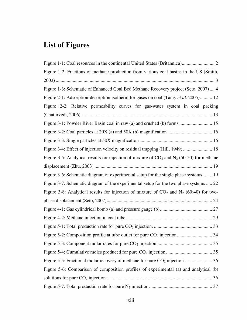
Relative permeability functions for gas-water system on coal have been found
experimentally by Chaturvedi (2006) and are shown in figure 2-2.
0
0.2
0.4
0.6
0.8
1
0 0.2 0.4 0.6 0.8 1
Water Saturation, Sw
Rel
ativ
e P
erm
eabi
lity
KrgKrw
Figure 2-2: Relative permeability curves for gas-water system in coal packing (Chaturvedi, 2006)

14
Numerical methods can be used to solve these flow equations and the ECBM process can
be simulated using commercial simulators. When using the standard first order upwind
discretization for transport, numerical diffusion may overwhelm any physical diffusion
present in the system. This may make it difficult to interpret the physics governing the
transport and production profiles. To achieve sufficient accuracy, a high level of grid
refinement is therefore required, which is generally computationally expensive for
compositional systems. Analytical solutions for the equations with the aforementioned
assumptions and under Riemann conditions can be useful in generating quick
approximate solutions. The validity of the simplifying assumptions and consequently
their conclusions can be investigated by performing laboratory experiments for one-
dimensional systems. Experiments also help in determining the feasibility of doing an
ECBM process depending on the physical and thermodynamic properties of the initial
system and the injection gas. The current work focuses on validating the analytical theory
by conducting both the laboratory-scale experiments as well as numerical simulations for
the multi-component, multi-phase flow for methane recovery from one-dimensional coal
packs (sections 3.4-3.6).

15
Chapter 3
3. Experimental Design
The aim of the project is to design and conduct experiments in order to improve
understanding of the governing mechanisms of enhanced coal bed methane recovery
processes in one-dimensional systems. The experiments are also used to validate the
simplifying assumptions made in the derivation of the analytical solutions for single and
multi-phase multi-component systems given in Zhu (2003) and Seto (2007). The
following sections describe the methodology of the experimental design.
3.1. Study of Coal Characteristics
The coal used in the study is lignite quality coal from Powder River Basin, Wyoming
(figure 3-1). It is ground into fine particles of size 50-60 mesh and stored under vacuum
to prevent its oxidation.
Figure 3-1: Powder River Basin coal in raw (a) and crushed (b) forms
The particle density of coal is measured to be 1466 kg/m3. Because coal particles are
compressible and adhesive, they show a wide range of size distribution as shown in figure
3-2.

16
Figure 3-2: Coal particles at 20X (a) and 50X (b) magnification
The crushed coal particles exhibit a dual porosity nature. The primary porosity is the void
space between particles and the secondary porosity is the intra-granular porosity within
the particles. A high magnification microscope image can capture the micro pores which
form the secondary porosity in coal as shown in figure 3-3.
Figure 3-3: Single particles at 50X magnification
The adsorption and desorption characteristics of the coal was previously studied by Tang
et al. (2005), and are reported to follow the Langmuir isotherm curve shown in figure 2-1.
The coal surface is micro porous and it exhibits diffusion within particles. Fick’s
diffusion model applies to coal particles and the diffusivities are reported to be of the
order of 10-5 - 10-9 cm2/s. For the particle size under consideration this diffusivity leads to
a diffusion time of 10-1 - 10-4 seconds in a single particle (Crank, 1957).
3.2. Slim tube configuration
Because the analytical studies so far were for one-dimensional systems, a slim tube
configuration is chosen. The length of the tube is chosen such that four pore volumes can
be passed through the tube in a run time of 8 hrs with a flow rate of 0.5 cc/min. For a

17
standard stainless steel tube of outer diameter 3/8” and thickness 0.035”, leading to an
inner diameter of 0.77 cm and a cross-sectional area of 0.4713 cm2, the length is
calculated to be
4.0*4713.0*460*8*5.0
**4* ==
φAtq
l = 318.2 cm = 3.18 m.
As this is an approximate calculation, a slim tube of 3 m length is used to do the
experiment.
The experiment is to be done vertically in order to avoid gravity effects. In cases of large
density difference between displacing and displaced fluid, gravity can be used to assist
displacement by countering the viscous effects like fingering. The tube, being long for the
height of laboratory, is bent at regular intervals in a zig-zag fashion.
3.3. Flow rate determination
In multi-phase studies, the mobility ratio plays an important role in determining the sweep
efficiency. In previous laboratory studies, several mechanisms were found to stabilize
solvent fingering. Under appropriate conditions, gravity can prevent viscous fingers from
forming. According to Hill (1949), solvent fingers will be completely dampened if the
frontal advance rate v, is less than or equal to the critical rate vc given by
min/0316.010
707.0*8.9*)1000(*)10*760(sin
3
15
cmgk
vc =≈∆∆= −
−
θµρ
, (2)
where � is the dip below horizontal, �� and �� are the density and viscosity differences,
respectively, between the displacing and the displaced fluid, and k is the Darcy
permeability of coal, which is discussed in chapter 5.
As a very small tube is needed to satisfy this bound on the velocity, which does not allow
the experiment to be conducted in a reasonable time, the injection is performed at a

18
higher rate. The resulting sweep inefficiency was studied by Hill (1949). His results are
shown in figure 3-4 below.
Figure 3-4: Effect of injection velocity on residual trapping (Hill, 1949)
The estimated flow rate of 0.5 cc/min falls in the range of v/vc between 10 and 100 for
which the residual saturation is between 10 and 20 percent of the pore volume.
3.4. Single phase experiments
Solutions to the Riemann problem have been obtained analytically for single phase
systems by Zhu (2003). The solutions obtained showed the presence of shocks and
rarefactions in the solutions for injection of pure and mixed gases. A typical displacement
is illustrated in figure 3-5. Experiments are conducted to validate the conclusions
(discussed in section 1.5) of the above analytical study. Figure 3-6 shows the
experimental setup for conducting single phase experiments. A brief description of
different components of the experimental setup is presented in Appendix A. The
following subsections discuss the different types of experiments conducted in this
category.

19
Figure 3-5: Analytical results for injection of mixture of CO2 and N2 (50-50) for methane displacement (Zhu, 2003)
Figure 3-6: Schematic diagram of experimental setup for the single phase systems
0.5 m
450
Gas Cylinder MFC
Pr Gauge
Valve 2
Methane saturated coal tube
Valve 1
BPR GC
Bubble Flow Meter
2-way Composition Profile

20
3.4.1. Binary displacement
The analytical work focuses on two main types of injection gases for displacement of
methane from coal. The first one is displacement with a more adsorbing and less volatile
gas than methane and the second is displacement with a less adsorbing and more volatile
gas than methane. These two experiments are conducted in the slim tube with two
different injection gases, CO2 and N2. CO2 is more adsorbing and less volatile than
methane, whilst N2 is less adsorbing and more volatile than methane. The operating
conditions for these experiments are listed in table 3-1. The coal tube is initially saturated
by injecting methane at a known pressure. Injection is done by controlling the rate at 25
cc/min at standard conditions and the production end is under pressure control with a
back pressure regulator. The back pressure is generally set close to the pressure at which
methane is initially injected in the coal. The back pressure is maintained high for two
reasons. Firstly, it helps in avoiding methane desorption from matrix space, so only the
methane from pore space is produced. Secondly, the pressure drop in the tube is small, so
the adsorption-desorption profile near the inlet is not very different from that near the
outlet of the tube.
3.4.2. Determination of dispersion coefficient
The results obtained from the single phase binary displacements are in agreement with the
analytical and numerical work done by Seto (2007) and Zhu (2003). They show the
presence of shocks and rarefactions for the two different injection scenarios discussed in
section 3.4.1. The spread of the front at the outlet is due to adsorption and dispersion of
gases in the coal pack. In the absence of adsorption, the spread of the front is an
indication of the convective dispersion and can be used to determine the dispersion
coefficient. An extra test is performed in which the tube is initially saturated with a non-
adsorbing gas in order to remove the effects of adsorption and to understand the
dispersion due to flow of gases in the pore space. Helium is known to be an inert gas with
negligible adsorption on coal, so coal is initially saturated with helium at a low pressure
and displacement is done with N2. N2 Injection is done from the bottom of the tube as it is

21
heavier than helium. The injection end is under rate control and the production end is
under pressure control. The operating conditions are listed in table 3-1.
3.4.3. Ternary displacement with mixture injection
Pure gases are not available at all the sites for performing ECBM, so a mixture of CO2
and N2 is tested as an injection gas to displace methane from coal tube in a displacement
study of gas phase systems. CO2 and N2 are mixed in a piston cylinder in the ratio of
55:45, keeping in mind that the analytical results in Zhu (2003) and Seto (2007) are
obtained for injection mixtures with 50:50 and 60:40 ratios of CO2 and N2 respectively.
The mixture is injected at a constant rate with the back end of the tube maintained at a
constant pressure. The operating conditions are listed in table 3-1.
Table 3-1: Operating conditions for single phase experiments
Injection Condition - Rate control (cc/min)
Initial Condition Injection Gas
Standard Conditions
Tube Pressure
Production Condition – Pressure Control (psia)
Methane at 440 psia
CO2 25 0.7 450
Methane at 480 psia
N2 25 0.357 500
Helium at 70 psia N2 2.6 0.7 72
Methane at 490 psia
CO2 + N2 (55:45)
25 0.7 475
3.5. Two-phase experiments
Analytical work has been done by Seto (2007) to solve the two-phase Riemann problem
for binary, ternary and quaternary systems with water as a mobile phase and component
of each system. The binary and ternary results led to similar conclusions of shock solution

22
for more adsorbing gas injection, rarefaction solution for less adsorbing gas injection and
chromatographic separation for mixture injection, as those obtained for the single phase
analytical (Zhu, 2003) and experimental studies (section 3.4). Seto’s results for
quaternary systems, which are initially saturated with water and methane, are obtained for
various compositions of the injection gas, which is composed of CO2 and N2. Validation
of these analytical results and conclusions about comparisons of saturated and under-
saturated systems is the motivation to extend the experimental work to two-phase
systems. Two-phase experiments are conducted with an initial water saturation in the pore
space and methane saturation in the matrix space and displacement is done for different
injection conditions. The experimental setup for two-phase systems is shown in figure 3-7
and the details of the setup are discussed in Appendix A.
Figure 3-7: Schematic diagram of the experimental setup for the two phase systems
0.5 m
450
Gas Cylinder MFC
Pr Gauge
Valve 2
Methane + water saturated coal tube
Valve 1
BPR GC
Bubble Flow Meter
2-way Valve Composition Profile
Water trap

23
3.5.1. Ternary displacement with pure CO2 injection
This experiment is conducted in a horizontal coal tube by first saturating it with methane.
Water is injected by constant pressure constraint from the inlet of the tube and the back
end of the tube is maintained at the same pressure at which methane was injected. Water
occupies the pore space by displacing methane. The matrix space is still occupied by
methane in its adsorbed state. The operating conditions for this experiment are listed in
Table 3-3. After saturating the tube to its initial condition, CO2 is injected at a constant
rate of 20 cc/min at standard conditions. The back end of the tube is maintained at a
constant pressure of 525 psia and not 725 psia at which the tube was initially saturated
with methane and water. This is because after the initial coal saturation at 725 psia, the
tube pressure reduced to 525 psia in the absence of any leakage. This is possibly due to
the dissolution of methane in water which reduced the pressure of the system.
3.5.2. Quaternary displacement with mixture injection
Analytical results for quaternary systems are obtained for various sets of injection gas
compositions. The fraction of CO2 in the injection mixture of CO2 and N2 is increased
from 0 to 1. A new composition path for certain injection gas compositions, depending on
the initial and thermodynamic state of the tube, is reported. The analytical result for a
60:40 injection mixture of CO2 and N2 representing this analytical solution is shown in
figure 3-8.
Table 3-2: Analytical vs realistic K values (Seto, 2007)
Analytical Real
KN2 5 417492
KCO2 1.2 1733
KCH4 3 50150
KWATER 0.1 0.0015

24
Figure 3-8: Analytical results for injection of mixture of CO2 and N2 (60:40) for two-phase displacement (Seto, 2007)
Figure 3-8 shows the presence of a degenerate shock from C-D which is a switch between
two non-tieline paths. A degenerate shock is one where the velocities immediately
upstream and downstream of the shock are equal to the shock velocity (Seto, 2007). This
two-phase quaternary experiment is conducted to see if this degenerate shock can be seen
in laboratory scale displacement in under-saturated coal by injection of a mixture of CO2
and N2. Even under same operating conditions, the results from experimental and
analytical studies are not expected to resemble due to inconsistencies in the physical
parameters. The analytical solutions are obtained for nonrealistic K values. The real K
values of CO2, N2 and methane are much higher, while that of water is much lower as
seen in table 3-2. Hence, in real the solubility of these gases in water is much lower.
Therefore, the size of the two phase region is larger. So, the compositional features seen
experimentally are expected to scale appropriately to the phase behavior of the system.
Similar to the experiment in section 3.5.1, this experiment has initial coal tube saturated
with water and methane. This experiment is conducted in a vertical tube with water
�

25
injection from the bottom of the tube at three different rates of 0.4, 0.1 and 0.05 cc/min.
The injection profile of water is shown in figure 5-26-a. After saturating the tube to its
initial condition, a mixture of CO2 and N2 in the ratio of 55:45 is injected from the top of
the tube at constant rates of 12 cc/min (standard conditions) at the beginning, then 2
cc/min and then 4 cc/min at the end of injection period The mixture injection profile is
shown in figure 5-29-a. The production end is controlled by the back pressure regulator at
300 psia (Due to pressure drop in the initial state of tube from 450 psia to 300 psia due to
dissolution of methane in water). The operating conditions for this experiment are listed
in Table 3-3.
Table 3-3: Operating conditions for two-phase experiments
Initial Condition
Injection Condition - Rate control (cc/min)
Water Injection Methane Injection
(psia) Injection Condition
Production Condition
Injection Gas
Standard Conditions
Tube Pressure
Production Condition –
Pressure Control (psia)
725 Pressure control – 775 psia
Pressure control – 725
psia
CO2 20 0.7 525
450 Variable rate
control – 0.4, 0.1,
0.05 cc/min
Pressure Control –
450
CO2 + N2
(55:45)
12, 2, 4 0.52, 0.1, 0.2
300
3.6. One-dimensional numerical simulation
Another way of validating the experimental results and also the analytical ones is by
numerical simulations. 1-D, finite-difference simulations with a fully implicit scheme are
performed using CMG’s commercial compositional simulator GEM (2006). From the
experiments, it is clear that physical dispersion (discussed in section 3.4.2) is infact

26
present in the system. But, since GEM does not allow it to be included, the physical
dispersion is modeled by using the numerics. So, a systematic approach of simulating
these systems with physical dispersion is followed. Using the experimental results, the
governing dispersion coefficient and Peclet number can be estimated. They are further
verified by analytical correlations (section 5.3). The Peclet number can be mimicked in
the numerical experiments if upwind methods are used to discretize transport. For the
standard first order upwind method (SPU) Lantz (1971) has shown that the numerical
diffusion coefficient can be computed using
���
����
�
∆∆−∆=−
ξτξ
12
1numPe . (3)
The spatial and temporal grid sizes can now be chosen such that the numerical Peclet
number equals the estimated physical Peclet numer. The ratio ξτ ∆∆ / must be taken so
as to satisfy the standard stability criteria as also discussed in Orr (2007).

27
Chapter 4
4. Operating Procedure
1. Determination of porosity and permeability
To find the porosity, a cylindrical bomb (figure 4-1-a) of 150 cc volume is pressurized
with helium at a known pressure P1. The coal tube is vacuumed for 24 hours and then
connected with the bomb with a valve in between the two. The valve is opened and the
final pressure P2 in the gauge (figure 4-1-b) is noted. This pressure corresponds to the
volume of bomb plus the pore volume of the coal tube plus any dead volume. The pore
volume can be found by using the relation
TTVPVP =11 , (4)
where
deadPoreT VVVV ++= 1 . (5)
ccV 1501 = , ccVdead 18.5= . P1 and PT are read from the gauge, so VT and Vpore are the
only unknowns and can be found by solving equations (4) and (5).
Several sets of these measurements are obtained and the data is tabulated in Appendix B.
The porosity of the coal tube is found to be 44%. It should be noted that this porosity
includes both the pore volume (roughly 34%) and the matrix porosity (roughly 10%) of
the coal pack (Resnik, 1984).
Figure 4-1: Gas cylindrical bomb (a) and pressure gauge (b)

28
Permeability is measured by performing simple Darcy experiments in the coal tube with
helium gas. Four pore volumes of helium are passed through the coal tube. The injection
and outlet pressures are observed and flow rate at the tube outlet is measured using the
bubble flow meter. The Darcy permeability is defined as
PAlq
k∆
=*
** µ, (6)
where q is the measured flow rate, µ is the viscosity of helium, l is the tube length, A is
the cross-sectional area of the tube and �P is the pressure drop across the length of the
tube.
Several sets of this measurement are obtained and the data is tabulated in Appendix C.
The permeability is found to be around 760 mD.
2. Vacuuming coal tube
After finding porosity and permeability or after doing one set of experiment, the tube is
put to vacuum for atleast 24 hrs. The weight of tube should come to that prior to
measuring porosity.
3. Purging coal tube with methane
As some of the components always remain on the coal surface due to its adsorbent
properties, the coal tube is purged with pure methane at high pressure after vacuuming
and the composition of the outlet gases is monitored in the GC. Methane is passed till the
chromatograph shows nearly100 % methane in the exit gas.
4. Injection of methane
After purging the tube, methane injection is continued at the desired injection pressure for
the experiment, with one end of the coal tube closed. The tube is weighed regularly in
order to determine the amount of methane injected. Injection should be done for atleast
24-48 hours even if the weight has stabilized. This is done in order to make sure that
methane does not remain only in free state but also gets adsorbed on surface of the coal.

29
0
0.4
0.8
1.2
1.6
0 20 40 60 80 100
Time (hrs)M
etha
ne in
ject
ed (g
ms)
Figure 4-2: Methane injection in coal tube
The volume of methane injected in the coal with time is shown in figure 4-2. This amount
can vary slightly for each experiment due to error made in the injection pressure gauge
and weighing balance. The injected methane is distributed in the coal pack both in the
pore space in free form and in the matrix space in adsorbed form. The individual amounts
can be computed by a material balance. The moles of methane present in the pore volume
i.e. the inter-granular space can be written as
TRz
VPn p
p **
*= , (7)
where P is the injection pressure, Vp is the inter-granular pore volume, z is the non-
ideality compressibility factor, R is the universal gas constant and T is the temperature.
The remaining moles are in the adsorbed state in the matrix porosity which can be found
by subtracting the moles in pore space, np, from the total moles injected, which is found
by weighing the tube.
5. Flow meter calibration
The flow meter is calibrated for each different gas being injected. The flow meter being
built for CO2 does not need to be calibrated for CO2 injection but needs calibration for N2
injection and the mixture injection.
6. Setting the back pressure

30
Before connecting the BPR to downstream end of the tube, it is set to the regulated
pressure as discussed in section 3.4 and 3.5, so that gas doesn’t escape before injection
begins after the BPR is connected to the coal tube.
7. Configuring the GC
The valve and column settings are adjusted in a way that the GC is able to separate the
components in the minimum possible time. Table 4-1 shows the setting for each
experiment:
Table 4-1: Method setup for running sequences in the GC
Exp
#
Components Run
time
(mins)
Columns used Valve setting Det
temp
(0C)
Oven
temp
(0C)
Carrier
gas rate
(ml/min)
Retention
time (mins)
1 CO2 + C1 5.3 Plot Q T=0, V3 on
T=5, V3 off
V2 always on
180 50 He – 4.8 CO2 - 3.64
C1 – 3.28
2 N2 + C1 6.4 Mol Sieve T=0, V3 on
T=0.1, V3 off
V2 always off
180 50,65 He – 4.8 N2 – 3.5
C1 – 4.1
3 He + N2 5.4 Mol Sieve T=0, V3 on
T=0.1, V3 off
V2 always off
180 50 H2 – 4.2 N2 – 3.13
He – 1.78
4 CO2 + N2 +
C1
10.23 Plot Q + Mol
Sieve
T=0, V3 on
T=3.4 , V2 on
T=4.2, V2 off
T=10, V3 off
180 50 H2 – 4.2 CO2 – 3.66
N2 – 7
C1 – 8.5
5 CO2 + N2 +
C1 + Water
10.23 Plot Q + Mol
Sieve
T=0, V3 on
T=3.4, V2 on
T=4.2, V2 off
T=10, V3 off
180 50 H2 – 4.2 CO2 – 3.66
N2 – 7
C1 – 8.5
A sequence table is set for automatic injections at regular interval which is analyzed using
the above configuration table called as a method in the GC software ChemStation (2006).
8. Starting gas injection

31
Once the set up is completed, the gas cylinder is turned on and the injection pressure is
adjusted automatically depending on the inlet flow rate and the back pressure. The
injection end is under rate control by the mass flow controller (MFC). The production end
is under pressure control by the back pressure regulator (BPR). The outlet valve of the
tube is opened first to check if the pressure in the tube is still maintained to what it was
saturated at. Then the inlet valve is opened for flow to begin in the tube. For water +
methane saturated initial conditions, the gas injection is done from top of the tube. In that
way gravity helps in preventing the fingering effect in a low viscosity fluid displacing a
high viscosity fluid system i.e. a high mobility ratio system.
9. Measurements
The following parameters are recorded during the injection period for the analysis and
interpretation of results:
• Injection pressure.
• Gas production rate.
• Produced gas composition.
• Water production in case of methane + water saturated initial condition.
10. Ending the experiment
Once all the injection gases have broken through and the flow rates have stabilized, the
injection is stopped and the valves are closed to measure the tube weight. Steps 2 through
10 are repeated for the next experiment.
11. Conducting two-phase experiments
After methane injection (step 4) at a known pressure, water is injected from the bottom of
the tube using the water pump at a fixed rate or fixed pressure. The back pressure
regulator is set at the end of the tube in order to avoid methane-escape by desorption. This
ensures that methane is displaced only from the free space and is produced at the tube
outlet. Once water sweeps through the tube, methane and water are co-produced and then

32
the water injection is stopped. Steps 5-10 are then conducted as in the single phase
experiments. The produced water is trapped in the water-trap and is measured in step 9.

33
Chapter 5
5. Results, Discussion and Material Balance
5.1. Results for pure CO2 injection for methane displacement
Pure methane is initially injected in the coal tube at 450 psia to get the system at an initial
condition saturated with methane. Pure CO2 is injected to displace this methane present in
both free state and adsorbed state. Methane is produced at the tube outlet and is followed
by CO2 production once the injected gas breaks through. Production of gases is monitored
and recorded to do a material balance check and the results are analyzed to understand the
displacement behavior of methane in coal by a more adsorbing gas.
CO2 is injected in the coal tube at 25 cc/min at standard conditions. Figure 5-1 shows that
production rate of gases at the outlet of the tube is around 12 cc/min till the time CO2
breaks through at the tube outlet. This is an indication of reduction in flow velocity due to
preferential adsorption of CO2 on coal over methane. As CO2 is transported in the coal
tube, for approximately three moles of CO2 adsorbed, only one mole of methane is
released, thereby leading to a reduction in volume and hence a decrease in velocity. As,
the CO2 front begins to appear at the tube outlet, the flow velocity increases. This is
because after all the adsorption has taken place, the flow is purely convective, so the
production rate comes to 25 cc/min which is also the injection rate.
Figure 5-1: Total production rate for pure CO2 injection.

34
Figure 5-2 shows the composition profiles of gases at the tube outlet vs pore volumes
injected (PVI). It can be seen that CO2 breaks through at around 2 PVI, which might seem
non-intuitive because as per mass conservation, for flow in a porous medium, the
injection gas should appear at the tube outlet after one pore volume is injected. But in this
case as CO2 gets adsorbed on coal, the volume of CO2 in free space reduces, hence the
need for more than one PVI to see the breakthrough. It can also be seen that CO2 breaks
through as a sharp front. This is because of the presence of a shock between the injection
and the initial tie line. This is in agreement with the analytical result for displacement by
an injection gas that is more adsorbing than the gas present initially.
Figure 5-2: Composition profile at tube outlet for pure CO2 injection
Figure 5-3 shows the individual component molar flow rates at the producing end of the
tube. By knowing the total volume flow rate and the composition of the production
mixture, the component molar rate is computed from ideal gas law as
min/*10*159.4293*314.8
*10**10132510* 566
gmolesxQxQ
RTPQx
n ccc
c−
−−
=== , (8)
where P is the pressure at which composition is measured in Pa, Q is the total production
rate in cc/min, xc is the mole fraction of the component c in the production mixture, R is
the universal gas constant and T is the tube temperature in K.

35
Figure 5-3: Component molar rates for pure CO2 injection
Figure 5-4 shows cumulative production of the components at the tube outlet. The
material balance is shown in table 5-1. It can be seen that almost all of the methane is
produced by the time CO2 breaks through. This also indicates that the CO2 front moves
very sharply inside the coal tube.
Figure 5-4: Cumulative moles produced for pure CO2 injection
Table 5-1: Material balance calculations for pure CO2 injection
Gmoles Gms Amount of methane injected initially (measured) 0.0925 1.48 Methane present in pore space (34% by volume) (Calculated) 0.0616 0.9856 Methane adsorbed in Matrix space (Calculated) 0.031 0.496 Amount of methane produced (measured) 0.0918 1.4688 Amount of CO2 trapped in coal (measured) 0.188 8.3

36
Figure 5-5: Fractional molar recovery of methane for pure CO2 injection
It can be seen from figure 5-5 that 90% of the methane present initially in the tube is
recovered at the time of CO2 breakthrough. The over all recovery is 100% as can also be
seen from the material balance check in table 5-1.
A result of this single phase experiment of methane displacement by CO2 in coal has been
obtained analytically by Zhu (2003). Figure 5-6 shows a comparison of experimental and
analytical results for methane and CO2 composition paths with non-dimensional wave
velocity. Figure 5-6 shows a good qualitative picture of the presence of a shock solution
from both the results. The results do not match perfectly in quantitative sense due to
differences in physical dispersion and adsorption of gases in the experimental and
analytical work. The analytical work assumes no dispersion to be present in this study
whereas the calculations in section 5.3 show a large physical dispersion.
Figure 5-6: Comparison of composition profiles of experimental (a) and analytical (b) solutions
for pure CO2 injection

37
5.2. Results for pure N2 injection for methane displacement
Similar to the above experiment, pure methane is initially injected in the coal tube at 480
psia to get the tube to methane-saturated initial state. Pure N2 is injected to displace this
methane and the production of gases are monitored and recorded.
N2 is injected in the coal tube at 25 cc/min at standard conditions. Figure 5-7 shows that
the production rate of gases at the outlet of the tube is around 32 cc/min till the time N2
breaks through at the tube outlet. N2 is more volatile and less strongly adsorbing than
methane so it travels quickly through the system, causing methane to desorb earlier than
when CO2 is injected. From the adsorption isotherm (figure 2-1) it can be seen that more
molecules of methane are desorbed for every molecule of N2 getting adsorbed. So,
volume is added to the flowing gas phase thereby increasing the flow velocity. As N2 is
produced at the tube outlet, the flow velocity gradually decreases to the injection velocity.
Figure 5-7: Total production rate for pure N2 injection
Figure 5-8 shows the composition profiles of gases at the tube outlet for N2 injection. It
can be seen that N2 breaks through at around 0.4 PVI, which gives an indication of an
increase in local flow velocity in the tube. This is due to the fact that injected gas is seen
at the outlet even before one pore volume is injected in the tube. This is just the reverse
effect of pure CO2 injection in which breakthrough occurs at 2 PVI. Also, another
observation is that the N2 front is highly dispersed as compared to the CO2 front in figure
5-2. This also blends well with the analytical study which predicts that displacement of

38
more strongly adsorbing and less volatile components by less strongly adsorbing and
more volatile components occurs through a continuous variation or a rarefaction wave.
Figure 5-8: Composition profile at tube outlet for pure N2 injection
The molar rates of individual components is shown in figure 5-9. It can be seen that the
rate of methane production is 1.3*10-3 gmoles/min for N2 injection as compared to 5*10-4
gmoles/min for CO2 injection case before breakthrough. As N2 propagates faster through
the tube, partial pressure of methane decreases, thereby leading to an early desorption and
hence a higher production rate of methane.
Figure 5-9: Component molar rates for pure N2 injection
Figure 5-10 shows the cumulative production of methane and it can be seen that even
after N2 breaks through, methane continues to produce. Hence there is a production of the
binary mixture which needs separation facilities.

39
Figure 5-10: Cumulative moles produced for pure N2 injection
The overall recovery of methane is 97% at 3 PVI as seen from figure 5-11 representing
the fractional recovery of methane for N2 injection. 40 % of methane is recovered at the
time of N2 breakthrough unlike the 90 % recovery of methane at CO2 breakthrough
(figure 5-5).
Figure 5-11: Methane recovery for pure N2 injection
The material balance calculations for N2 injection are shown in table 5-2.
Table 5-2: Material balance calculations for N2 injection
Gmoles Gms Amount of methane injected initially (measured) 0.1 1.6 Methane present in pore space (34% by volume) (Calculated) 0.0657 1.0512 Methane adsorbed in Matrix space (Calculated) 0.034 0.544 Amount of methane produced (measured) 0.097 1.552 Amount of N2 trapped in coal (measured) 0.073 2.052

40
Figure 5-12 shows a comparison of the results from the analytical work of Zhu (2003)
and the experimental work for methane displacement in coal by N2. Again, the numerical
values of breakthrough time and the extent of the dispersed front do not match but both
the results are in agreement with the proposed theory of the presence of a rarefaction
wave between the initial and injection tie lines for this kind of displacement.
Figure 5-12: Comparison of composition profiles of experimental (a) and analytical (b) solutions
for pure N2 injection
5.3. Results for dispersion experiment
The dispersed fronts seen in sections 5.1 and 5.2 led to the conduction of a tracer test in
which the tube is initially saturated with helium which is then displaced with N2. The
composition profile is shown in figure 5-13.
Figure 5-13: Helium fraction in the produced gas

41
The dispersion coefficient Kl is made up of the combined effects of molecular diffusion
and fluid flow in the pore space. It can be calculated using a correlation given by Perkins
and Johnston (1963) given as
00
*75.1
1D
dU
FDK pl +=
φ, (9)
where Do is the molecular diffusion coefficient, U = 0.024 cm/sec is the flow velocity, dp
= 0.025 cm is the particle diameter and 7.0/1 =φF (Perkins and Johnston, 1963).
Rohling et al. (2007) reported a molecular diffusion coefficient of N2 in helium, to be
0.698 cm2/sec at ambient conditions. The molecular diffusion coefficient can be
calculated at the tube pressure using ≈PDo Constant (Perry and Green, 2007). So, Do at
70 psia is approximately 0.146 cm2/sec and the dispersion coefficient, Kl is thus found to
be 0.1022 cm2/sec.
The dispersion coefficient can also be calculated using the analytical theory as described
in Orr (2007) as
���
����
� −=τ
τξ2
)(21 Pe
erfcc , (10)
where c is the volume fraction of a component, /x Lξ = , Lut φτ /= and lKuLPe φ/= .
The dispersion coefficient can be found by creating a plot in the arithmetic probability
coordinates using ( )berfcc =2 . Taking the inverse of both sides, equation (10) becomes
1(2 )erfc c b− = .
The argument on the right hand side can be evaluated at 1ξ = , the core outlet, where the
concentration is measured. Now (10) becomes
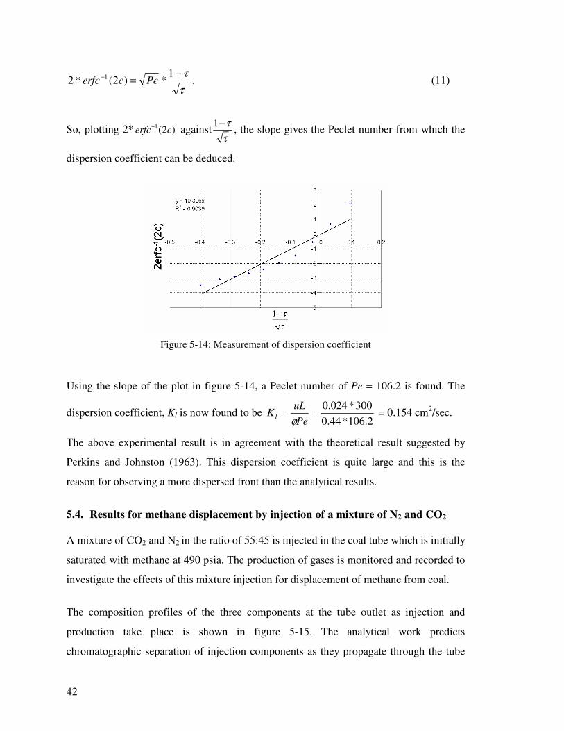
42
ττ−=− 1
*)2(*2 1 Pecerfc . (11)
So, plotting 2* 1(2 )erfc c− against 1 ττ
− , the slope gives the Peclet number from which the
dispersion coefficient can be deduced.
Figure 5-14: Measurement of dispersion coefficient
Using the slope of the plot in figure 5-14, a Peclet number of Pe = 106.2 is found. The
dispersion coefficient, Kl is now found to be 2.106*44.0
300*024.0==PeuL
K l φ = 0.154 cm2/sec.
The above experimental result is in agreement with the theoretical result suggested by
Perkins and Johnston (1963). This dispersion coefficient is quite large and this is the
reason for observing a more dispersed front than the analytical results.
5.4. Results for methane displacement by injection of a mixture of N2 and CO2
A mixture of CO2 and N2 in the ratio of 55:45 is injected in the coal tube which is initially
saturated with methane at 490 psia. The production of gases is monitored and recorded to
investigate the effects of this mixture injection for displacement of methane from coal.
The composition profiles of the three components at the tube outlet as injection and
production take place is shown in figure 5-15. The analytical work predicts
chromatographic separation of injection components as they propagate through the tube
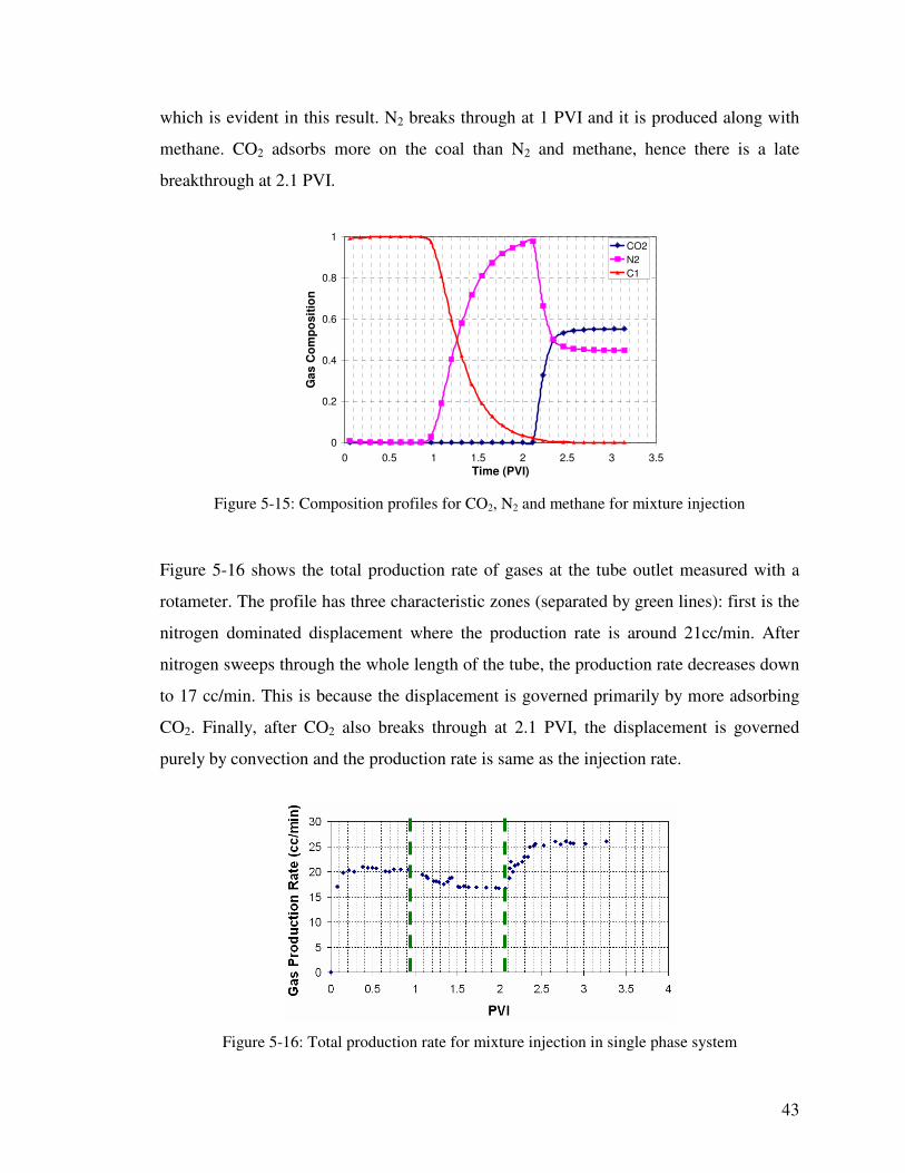
43
which is evident in this result. N2 breaks through at 1 PVI and it is produced along with
methane. CO2 adsorbs more on the coal than N2 and methane, hence there is a late
breakthrough at 2.1 PVI.
0
0.2
0.4
0.6
0.8
1
0 0.5 1 1.5 2 2.5 3 3.5Time (PVI)
Gas
Com
posi
tion
CO2N2C1
Figure 5-15: Composition profiles for CO2, N2 and methane for mixture injection
Figure 5-16 shows the total production rate of gases at the tube outlet measured with a
rotameter. The profile has three characteristic zones (separated by green lines): first is the
nitrogen dominated displacement where the production rate is around 21cc/min. After
nitrogen sweeps through the whole length of the tube, the production rate decreases down
to 17 cc/min. This is because the displacement is governed primarily by more adsorbing
CO2. Finally, after CO2 also breaks through at 2.1 PVI, the displacement is governed
purely by convection and the production rate is same as the injection rate.
Figure 5-16: Total production rate for mixture injection in single phase system

44
Similar to pure gas injection, the production molar rates of individual components are
calculated by applying the ideal gas law and then the cumulative production of gases in
moles are calculated. The results are shown in figure 5-17.
0.0E+00
2.0E-04
4.0E-04
6.0E-04
8.0E-04
1.0E-03
0 0.5 1 1.5 2 2.5 3 3.5
Pore Volumes Injected
Pro
duct
ion
Mol
ar R
ate
(gm
oles
/min
) Exp-C1Exp-CO2Exp-N2
0
0.02
0.04
0.06
0.08
0.1
0 0.5 1 1.5 2 2.5 3 3.5
Pore Volumes InjectedC
umul
ativ
e M
oles
pro
duce
d (g
mol
es)
Exp-C1Exp-CO2Exp-N2
Figure 5-17: Production profiles for mixture injection
Figure 5-18 shows that 75% of the original methane in place is recovered by the time
nitrogen breaks through and the overall recovery is 95%.
0
0.2
0.4
0.6
0.8
1
0 0.5 1 1.5 2 2.5 3 3.5
Pore Volumes Injected
Frac
tiona
l Mol
ar R
ecov
ery
Figure 5-18: Methane recovery for mixture injection in single phase system
The material balance calculations for the mixture injection are shown in table 5-3.
Table 5-3: Material balance calculations for mixture injection in single phase system
Gmoles Gms Amount of methane injected initially (measured) 0.100625 1.61 Methane present in pore space (34% by volume) (Calculated) 0.067 1.072 Methane adsorbed in Matrix space (Calculated) 0.0336 0.538 Amount of methane produced (measured) 0.09404 1.5046 Amount of (CO2 + N2) trapped in coal (measured) 5.81

45
A good qualitative comparison between the analytical (0.5 CO2 + 0.5 N2, Zhu (2003)) and
experimental (0.55 CO2 + 0.45 N2) results can be seen in figure 5-19. The experimental
observations show a clear nitrogen bank being produced with methane and the shock
solution for CO2 composition as depicted in the analytical results.
Figure 5-19: Comparison of composition profiles of experimental (a) and analytical (b) solutions
for mixture injection in single phase systems
5.5. Comparison of the single phase experiments with different injection gases
Figure 5-20: Experimental results for Methane recovery by different injection gases

46
Figure 5-20 shows the recovery profiles for the cases of pure CO2, the mixture of CO2
and N2 (0.55 CO2 + 0.45 N2) and pure N2 injection to displace methane from the coal
tube. It can be seen that as the CO2 concentration in the injection gas increases, the rate of
recovery decreases. The overall recovery varies from 95 % to 99 %.
Figure 5-21: Experimental results for total production rate with different injection gases
Figure 5-21 shows the total production rate at the tube outlet for the three cases. The total
production rate is 12 cc/min in the pure CO2 injection case before the break through of
CO2 where as in the pure N2 injection case the total production rate is 32 cc/min before
N2 breaks through. In the mixture injection case, the production rate is 21 cc/min initially
until N2 breaks through and then reduces to 17 cc/min until CO2 breaks through. The
three results show that N2, being less adsorbing than methane, passes quickly through the
tube leading to reduction of partial pressure of methane and subsequent desorption and
higher flow rate. On the other hand, the presence of CO2 tends to slow down the front
velocity. CO2 is preferentially adsorbed on coal over methane so the volume flow rate
decreases. Finally, after all the injection gases break through, the three profiles for
production rates come to the same value as the injection rate which is 25 cc/min as seen
in figure 5-21.

47
Figure 5-22: Experimental results for methane production rate by different injection gases
Figure 5-22 shows the methane production rate for the three cases. As explained above, it
can be seen that the methane production rate decreases as the CO2 fraction in the injection
gas increases. Also, it is interesting to note the shape of fronts for the three cases. CO2
injection leads to a sharper front (shock solution) where as N2 injection leads to a smooth
transition (rarefaction solution).
5.6. Results for displacement of water and methane by pure CO2 injection
The production rate at the tube outlet is not measured in this case. Only the composition
of the exit gases is measured with the gas chromatograph and is shown in figure 5-23.
Breakthrough of CO2 occurs at 1.8 PVI. The figure also shows that the CO2 moves as a
sharp front. Almost all of the methane is recovered by the time CO2 breaks through.
0
0.1
0.2
0.3
0.4
0.5
0.6
0.7
0.8
0.9
1
0 0.5 1 1.5 2 2.5 3 3.5
Time (PVI)
Com
posi
tion
CO2C1
Figure 5-23: Composition profile for CO2 injection in coal with methane and water saturation

48
Figure 5-24 shows the fractional water recovery. There was no production of water
initially as the back pressure of the tube went below the controlled design pressure of 600
psia. As the pressure built up, water production started and a total of 35 % of the water
was recovered from the tube.
0
0.1
0.2
0.3
0.4
0 0.5 1 1.5 2 2.5 3 3.5
PVI
Frac
tion
of w
ater
pro
duce
d
Figure 5-24: Fractional water production for CO2 injection in methane and water saturated coal
Figure 5-25 shows a comparison of the analytical (Seto, 2007) and experimental results
for gas phase compositions of methane and CO2. The breakthrough times for both the
cases are around 0.45 in terms of the dimensionless wave velocity. The experimental
results show a more dispersed front than the analytical results due to the presence of
physical dispersion discussed in section 5.3. Another reason is because the analytical
results are obtained for nonrealistic K values and solubilities for the two-phase system as
shown in table 3-2.
Figure 5-25: Comparison of experimental (a) and analytical (b) results for pure CO2 injection in water + methane saturated system

49
5.7. Results for displacement of water and methane by mixture injection
The tube is initially saturated with methane. The amount of methane in the pore space and
in the matrix is calculated as described before. Water is injected to displace the methane
in the pore space. Methane in the matrix space remains adsorbed because the back
pressure is maintained at the adsorption pressure of methane. This brings the system to its
initial state.
Water Injection
0
10
20
30
40
50
60
70
0 100 200 300 400 500 600 700Time (mins)
Wat
er In
ject
ed (c
c)
0
1
2
3
4
5
6
7
8
9
10
Wat
er P
rodu
ced
(cc)
injectionproduction
0
10
20
30
40
50
60
70
0 0.2 0.4 0.6 0.8 1 1.2Time (PVI)
Wat
er In
ject
ed (c
c)
0
1
2
3
4
5
6
7
8
9
10
Wat
er P
rodu
ced
(cc)
injectionproduction
0
10
20
30
40
50
60
70
0 100 200 300 400 500 600 700
time (mins)
wat
er in
ject
ed (c
c)
0
0.01
0.02
0.03
0.04
0.05
0.06
0.07
0.08
prod
uced
gas
(gm
oles
)
water injectedcum gas produced
0
10
20
30
40
50
60
70
0 0.2 0.4 0.6 0.8 1 1.2
Time (PVI)
wat
er in
ject
ed (c
c)
0
0.01
0.02
0.03
0.04
0.05
0.06
0.07
0.08
prod
uced
gas
(gm
oles
)
water injectedcum gas produced
Figure 5-26: Injection and production profiles for water injection
A total of 0.105 gmoles of methane are injected in the tube initially and then water is
injected at variable rates of 0.4, 0.1 and 0.05 cc/min at tube pressure. The variable
injection rates can be seen in figure 5-26-a as a function of time. In figure 5-26-b water
injection and production are plotted as a function of pore volumes injected so the effect of
rate does not show up in the graph. Water is produced after 1 PVI, which is an indication
a b
c d

50
that water has swept all the pore space. It should be noted here that the pore space refers
to inter-granular porosity (total porosity – matrix porosity). After breakthrough, water is
produced at the same rate as the injection rate, which is 0.05 cc/min. Methane is produced
through out the water injection time as seen from figure 5-26-c. It can be seen that
methane production rate is also affected by the water injection rate. As the water injection
rate is decreased, the methane production rate also decreases. It can be seen from figure 5-
27-a that as the water breaks through, the gas rate comes to zero sharply, also indicating
the sharpness of water front in the tube.
0
2
4
6
8
10
12
14
16
0 0.2 0.4 0.6 0.8 1 1.2Time (PVI)
Gas
Pro
duct
ion
Rat
e (c
c/m
in)
0
1
2
3
4
5
6
7
8
9
10
wat
er p
dn (c
c)gas pdn Ratewater pdn
0
0.1
0.2
0.3
0.4
0.5
0.6
0.7
0.8
0 0.2 0.4 0.6 0.8 1 1.2Time (PVI)
Frac
tion
of m
etha
ne p
rodu
ced
Figure 5-27: Production profiles for water injection in methane saturated coal
Figure 5-27-b shows the fraction of methane released from the tube as water is injected.
73% of the total methane in place is produced by water injection. This is the volume of
methane which is calculated to be present in the pore space prior to water injection as
shown in the material balance check in table 5-4. Because methane is produced only from
the pore space, the produced volume also validates of the assumed porosity distribution
between pore space and matrix space of 34% and 10 % respectively. Material balance
calculations for water injection in methane-saturated tube are shown in table 5-4.
a b

51
Table 5-4: Material balance calculations for water injection in methane saturated coal
Gmoles Gms Amount of methane injected initially @ 500 psia (measured) 0.105 1.68 Methane present in pore space (34% by volume) (Calculated) 0.0684 1.0944 Methane adsorbed in Matrix space (Calculated) 0.0365 0.5848 Total methane left after pressure reduction to 420 psia due to connecting water pump
0.094 1.5046
Amount of methane produced (measured) 0.068 1.093 Amount of water in the tube (= injected-produced-dead volume) (measured)
2.44 44
Amount of methane left in the tube 0.025 0.4116
Gas Mixture injection
Mixture of CO2 and N2 (0.55:0.45) is initially injected at a flow rate of 12 cc/min at
standard conditions to displace the methane and water from the coal. No gas was
produced for the first quarter of pore volume injected. This is because the pressure in the
tube was lower than the designed back pressure. As the gases begin to produce, N2 is
detected in the exit gases (figure 5-28). The early breakthrough of N2 may be because of
the unstable displacement velocity. The mobility ratio for this system, with gas and water
viscosities of the order of 0.01 cp and 1 cp respectively, is around 100. Due to this large
mobility ratio there is fingering effect in the coal due to which N2 flows quickly through
the pores.
Figure 5-28: Composition profile of exit gases for mixture injection

52
The injection rate is reduced to 2 cc/min after 0.8 pore volumes are injected and further
increased to 4 cc/min after 1.5 PVI. The gas production rate is seen to follow the injection
profile as seen in figure 5-29-a. Initially a high production rate is seen, then the rate
decreases and finally increases up to the injection rate of 4 cc/min at standard conditions.
Figure 5-29: Injection and production profiles
The cumulative production is shown in figure 5-29-b. A large volume of N2 is produced
due to its early break through as seen in figure 5-28. Methane is also produced with N2, so
needs to be separated from the mixture for commercial uses. Sharp changes are seen in
the composition profiles due to changes in the injection rate.
Figure 5-30: Water and methane recovery for mixture injection in two-phase system
The overall recovery of methane is 100% and only 23% of original water is produced
(figure 5-30). Low water production is likely caused by an unstable displacement front in
the tube. So, from an ECBM point of view, a higher injection rate than the critical
a b

53
velocity (determined in section 3.3) can still be a feasible approach as all the methane is
still recovered. However, this large production comes at the cost of large injection
volumes of CO2 and N2. Also, the produced gas is mostly a mixture of N2 and methane,
which need to be separated. Material balance calculations for mixture injection in a tube
saturated with water and methane are shown in table 5-5.
Table 5-5: Material balance for mixture injection in water + methane saturated coal
Gmoles Gms Amount of water injected (measured) 2.44 44 Amount of methane left in the tube (calculated) 0.0257 0.4116 Amount of methane released (measured) 0.0256 0.4096 Amount of water produced (measured) 0.62 11.17 Amount of (CO2+N2) trapped in coal (calculated) 2.05
Composition profiles for the four components are plotted for the experimental and the
analytical study (Seto, 2007) in figure 5-31. The experimental solutions are more
dispersed than the analytical ones but it is interesting to note some of the common
features. The analytical result shows the presence of a degenerate shock for this
composition of the injection gas (Type III-C: 0.6 CO2 + 0.4 N2). Two sharp peaks can be
seen in the experimental results for N2. One of them is possibly due to the degenerate
shock. A shock solution for CO2 can also be seen but as a more dispersed front which is
due to the large dispersion coefficient calculated in section 5.3. The numerical values of
solution compositions are different as the analytical study is done for non-real K values
and solubility data of liquids and gases as shown in table 3-2.

54
Figure 5-31: Comparison of experimental (a) and analytical (b) results for mixture injection in
water + methane saturated system
5.8. Effects of saturated and under saturated initial conditions and comparison with analytical solutions
Another important part of the analytical study done by Seto (2007) is the comparison
between saturated and under saturated systems. Saturated systems are defined as the ones
having significantly large volumes of methane trapped in coal (more than 30% of mixture
on molar basis). Under-saturated systems are defined as ones in which less methane is
available to be recovered (0.05% of mixture).
In the experimental study, a similar comparison can be made between systems with a
large quantity of methane (single phase systems with pure methane) referred to as
saturated and the ones having a small volume of methane trapped in coal (methane
(0.04%) + water saturated coal) referred to as under-saturated system. The analytical
study proposes a banking behavior in the methane profile in under-saturated system. This
is seen as the red curve in figure 5-32 in the methane profiles of both the analytical and
experimental results. Also, the small leading shock in CO2 profile is clearly visible in the
experimental results in figure 5-32-a. Again, this is a good qualitative match but not a

55
quantitative assessment due to different parameters, mainly the K values (table 3-2) and
the dispersion coefficient (section 5.3), used in the two studies.
Figure 5-32: Comparison of experimental (a) and analytical (b) solutions for saturated and under-
saturated systems
Another result of comparison between saturated and under-saturated systems is from the
CO2 sequestration point of view. The analytical study proposes more CO2 to be injected
into the reservoir prior to the gas break through in under-saturated coals. Material balance
check (table 5-6) for the pure CO2 injection experiments in systems with and without
water shows the same result. Figure 5-33 shows the composition profiles of the exit gases
for the two systems. It should be noted that the under-saturated (with water) experiment
was conducted at a higher pressure of 725 psia where as the saturated (without
water/single phase) experiment was conducted at 450 psia. So, even though the saturated
system shows a late break through of CO2, the material balance check (table 5-6) shows
that 27 % more CO2 is injected in the under-saturated coal as compared to the saturated
coal.

56
Figure 5-33: Composition profiles of CO2 in saturated and undersaturated systems
Table 5-6: Material balance for CO2 capture in saturated and under-saturated systems
Volume at tube pressure (cc) Volume at STD (cc) Unsaturated initial condition 100 @ 720psia 4897 Saturated initial condition 126 @ 450 psia 3857
5.9. Numerical study of ECBM recovery
Numerical simulations are done to further validate the experimental and the analytical
observations. As discussed in section 3.6, the dispersion experiment is simulated first by
including some numerical diffusion in the discretization scheme. In case of no physical
dispersion in the system, the converged solution should give a sharp front. As the
numerical Peclet number is increased, the solution front gets sharper, which can be seen
in figure 5-34.

57
Figure 5-34: Convergence test for dispersion experiment
The dispersed experimental solution seen in section 5.3 is obtained by matching the
numerical diffusion to the physical dispersion. Starting from Pe = 1300, both the space
and time discretization are coarsened while keeping ξτ dd / = 0.1. A good match is
obtained for a numerical Peclet number of 200 (figure 5-35). The best fit straight line in
figure 5-14 gave a Peclet number of 106. The discretization parameters are listed in table
5-7.
Figure 5-35: Effect of increasing the numerical diffusion
Table 5-7: Discretization parameters for dispersion experiment
Peclet Number, Pe ξτ dd / Number of grid blocks x∆ (m) t∆ (min)
200 0.1 90 0.033 0.101

58
The match between experimental and numerical result for this discretization is shown in
figure 5-36. The data file for this simulation result is attached in Appendix D.
Figure 5-36: Composition profile for dispersion experiment
Following the same approach of including some numerical diffusion, other experiments
are also simulated by using the fully implicit discretization method in the GEM simulator.
The dual porosity model with matrix and fracture regions is used to simulate the actual
flow in the coal tube. The adsorption parameters and PVT properties of the participating
components are assigned and the coal properties like density and compressibility are
assigned for the two regions.
5.9.1. Simulation of methane displacement by pure CO2
The production rate shown in figure 5-37-a is matched by supplying the adsorption data
(figure 2-1) to the simulator. Maximum adsorption of methane on coal is set to be 0.625
gmol/kg of rock, maximum adsorption of CO2 is set as 2.8 gmol/kg of rock and the
inverse pressure parameter is 1.61*10-4 KPa-1. It should be noted that the simulation
result is very sensitive to the adsorption data. The breakthrough time and the production
rate are both directly related to the adsorption of the gas species. A more adsorbing
injection gas leads to a late breakthrough and a slower production rate. Thus, the
adsorption data influences the numerical solutions.

59
Figure 5-37: Simulation and experimental comparisons for pure CO2 injection
The spread of the front as seen in figure 5-37-b is matched by using a numerical Peclet
number of 100. This also compares well with the physical Peclet number found as 106.
The discretization parameters are listed in table 5-8.
Table 5-8: Discretization parameters for pure CO2 injection in methane saturated coal
Peclet Number, Pe ξτ dd / Number of grid blocks x∆ (m) t∆ (min)
100 0.2 40 0.075 0.457
5.9.2. Simulation of methane displacement by pure N2
The production rate shown in figure 5-38-a is matched by supplying the adsorption data
(figure 2-1) to the simulator. Maximum adsorption of methane on coal is set to be 0.625
gmol/kg of rock, maximum adsorption of N2 is set as 0.227 gmol/kg of rock and the
inverse pressure parameter is 1.61*10-4 KPa-1. The discretization parameters are listed in
table 5-9.
Table 5-9: Discretization parameters for pure N2 injection in methane saturated coal
Peclet Number, Pe ξτ dd / Number of grid blocks x∆ (m) t∆ (min)
133 0.249 50 0.06 0.457
a b

60
It should be noted from table 5-9 that the number of grid blocks is brought down to 50 to
match the dispersed front. The convergence study shows a Peclet number of around 1300
for the converged solution which corresponds to around 700 grid blocks. This indicates
the significant amount of dispersion present in the system as discussed in section 5.3.
Figure 5-38: Simulation and experimental comparisons for pure N2 injection
The numerical Peclet number for this case also matches very well with the physical Peclet
number and the production data also matches well with the numerical result as shown in
figure 5-38.
5.9.3. Simulation of methane displacement by mixture of CO2 and N2
The same adsorption parameters as in section 5.9.1 and 5.9.2 are supplied to the simulator
for the ternary system of mixture injection. The discretization parameters are listed in
table 5-10.
Table 5-10: Discretization parameters for mixture injection in methane saturated coal
Peclet Number, Pe ξτ dd / Number of grid blocks x∆ (m) t∆ (min)
108.52 0.08 50 0.06 0.144
In this case also, a significant numerical diffusion is present as the Peclet number is
108.52. The numerical solution is in good agreement with the experimental results as
seen in figure 5-39.

61
Figure 5-39: Simulation and experimental comparisons for mixture injection

62
Chapter 6
6. Conclusions
The experimental results are obtained for binary, ternary and quaternary systems and are
compared with the analytical and the numerical results. The following conclusions can be
drawn from the comparison of these results:
1. Significant dispersion is present in gas phase systems as shown in section 5.3. The
dispersion coefficient is 0.154 cm2/sec. The large dispersion in the tube leads to
more dispersed front of the injection gases as compared to the analytical solutions.
2. As predicted in the analytical study, the displacement of methane by a more
adsorbing gas occurs via a shock solution between the injection and the initial
compositions. This can be seen in figure 5-2 where the composition change
interval for methane and CO2 lies within 0.3 pore volume injections.
3. As predicted in the analytical study, the displacement of methane by a less
adsorbing gas occurs via a rarefaction wave between the injection and initial
compositions. The composition profiles vary smoothly for both the components as
seen in figure 5-8. The composition change interval for N2 and methane lies in a
1.5 pore volume injection period. The comparison between the analytical and
experimental work shown in figure 5-12 also shows the same characteristics of a
rarefaction wave.
4. The solutions from the experimental results for the displacements by pure CO2
and pure N2 are more dispersed than the analytical solutions because of the large
dispersion coefficient and nonrealistic K-values used in the analytical study.

63
5. Displacement of methane by a more adsorbing gas occurs slowly due to volume
reduction. This can be seen in figure 5-1, where the production rate is smaller than
the injection rate until CO2 breaks through.
6. Displacement of methane by a less adsorbing gas occurs faster due to an increase
in the volume. This can be seen in figure 5-7, where the production rate is larger
than the injection rate till the time N2 breaks through.
7. Displacement of methane by a mixture of gases (more adsorbing and less
adsorbing than methane) shows three prominent stages of production (figure 5-
16). The first stage is controlled by N2 production at a rate depending on the
concentration of N2 in the injection mixture. Next stage is controlled by CO2
production at a rate lower than the previous stage due to more adsorption of CO2
than methane. The third stage is purely due to convection where the rate of
production equals the injection rate.
8. Displacement by a more adsorbing gas is slower than the displacement by a less
adsorbing gas and that by a mixture of the two occurs at a rate between the
displacements by individual gases. This can be seen in figure 5-22 where the
methane production rate for the three types of injection gases is shown. As CO2
concentration in the injection gas increases, the production rate decreases.
9. Two-phase experiments should be conducted at a very small rate in order to have
a stable front displacement. The early breakthrough of N2 seen in figure 5-28 and
low water production (figure 5-30) are a result of the unstable front.
10. The experimental results shown in figure 5-31, confirm the presence of a
degenerate shock in the solution profile for the particular mixture injection in the
two-phase system. This validates the analytical theory as suggested by Seto
(2007).

64
11. A banking behavior in the methane composition profile and a small leading shock
for the CO2 profile for under-saturated systems are validated by experimental
results for saturated and under-saturated systems as shown in figure 5-32.
12. More CO2 is trapped when the initial state of coal is under-saturated as shown by
material balance in table 5-6. So, under-saturated systems are better from CO2
sequestration point of view.
13. Numerical models can be constructed to represent the actual physical dispersion in
the coal by including numerical diffusion of the order of the actual dispersion
present in the system. The numerical Peclet numbers are in good agreement with
the physical dispersion and the solution profiles from the numerical models are in
good agreement with the experimental results.

65
Nomenclature
A : Cross Sectional area of coal tube
ai : Amount of component i adsorbed on per unit volume of coal
c : Volume fraction of a component
Do : Molecular diffusion coefficient
dp : Particle diameter
g : Gravitational constant
k : Permeability of coal packing
Kl : Dispersion coefficient in coal
Krg : Gas relative permeability
Krw : Water relative permeability
l : Length of coal tube
np : Moles of methane in inter-granular porosity
Pe : Peclet number
pi : Partial pressure of component i
q : Volume flow rate
R : Universal gas constant
Sj : Saturation of phase j

66
T : Temperature of the coal tube
uj : Local flow velocity of phase j
U : Flow velocity in the tube
v : Injection velocity
V1 : Volume of cylindrical bomb
vc : Critical velocity for stable flow
Vdead : Dead volume of the coal tube
Vmi : Langmuir constant at specified temperature Bi for component i
Vp : Volume of the inter-granular pore space
Vpore : Total volume of the pores in coal tube
VT : Total volume of bomb + pore volume + dead volume
xij : Mole fraction of component i in phase j
z : Non-ideality compressibility factor
Greek Symbols
ξ : Dimensionless distance
τ : Dimensionless time
� : Dip angle below horizontal
�� : Density difference between displacing and displaced fluid

67
�� : Viscosity difference between displacing and displaced fluid
�P : Pressure drop across length of the coal tube
φ : Porosity of the medium
�j : Molar density of phase j
�r : Mass density of coal bed

68
References
Britannica Encyclopedia, Inc. Online at http://www.britannica.com/eb/art-1626
Chabak, J., Yee, D., Volz, R. F., Seidle, J. P., Puri, R. :“Method for Recovering
Methane from Solid Carbonaceous Subterranean Formations,” U.S. Patent (1996) 5
566 756
Chaturvedi, T. :“Spontaneous Imbibition and Wettability Characteristics of Powder
River Basin Coal,” Master’s Report, Stanford University (2006). Online at
http://pangea.stanford.edu/ERE/pdf/pereports/MS/Chaturvedi06.pdf
ChemStation :“Understanding Your ChemStation” Gas Chromatograph Software
User Manual Number G2070-91123, Agilent Technologies (2006)
Close, J. C. AAPG Studies in Geology: Natural Fractures in Coal. (1993) 38, 119-132
Crank, J. :“The Mathematics of Diffusion” Oxford at the Clarendon Press, N.Y.
(1957)
Every, R. L., Dell’osso, Jr., L., :“A New Technique for the removal of methane from
Coal,” Canadian Mining and metallurgy Bulletin (March 1972)
Fulton, P. F., Parente, C. A., Rogers, B. A., Shah, I., Reznik, A. A. :“Laboratory
Investigation of Enhanced Recovery of Methane from Coal by Carbon Dioxide
Injection,” paper SPE 8930 presented at the SPE/DOE Symposium on
Unconventional Gas Recovery held in Pittsburg, PA, 18-21 May 1980

69
Garduno, J. L., Morand, H., Saugier, L., Ayers, W. B., McVay, D. A. :“CO2
Sequestration Potential of Texas Low-Rank Coals” paper SPE 84154 presented at the
SPE Annual Technical Conference and Exhibition, Denver, CO, 5-8 October 2003
GEM :“Generalized Equation-of-State Model” Compositional Reservoir Simulator,
Computer Modelling Group Ltd., Version 2006.1 (2006)
Gunter, W. D., Genetzis, T., Rottenfuser, Richardson, R. J. H. :“Deep coalbed
methane in Alberta, Canada. A fuel resource with the potential of zero greenhouses
gas emissions,” Energy Conservation and Management (1997), 38, S: 217–222
Hesse, M. A., Tchelepi, H. A., Cantwell, B. J., Orr, F. M., Jr. :“Gravity currents in
horizontal porous media: Transition from early to late self-similarity,” J. Fluid
Mechanics (2007), 577, 363 - 383
Hill, S.: “Channeling in Packed Columns,” Chem. Eng. Sci. (1949) 1, No. 6, 247
Johansen, T., Tveito, A., Winther, R., Dahl, O. :“Multicomponent Chromatography in
a Two Phase Environment,” SIAM J. Appl. Math. (1992) 52, no. 1, 65-104
Lantz, R. B. :“Quantitative Evaluation of Numerical Dispersion (Truncation Error),”
Soc. Pet. Eng. J. (1971) 11, 315
Levine, J. R. AAPG Studies in Geology: Coalification: The Evolution of Coal as a
Source Rock and Reservoir Rock for Oil and Gas. (1993) 38, 39-77.

70
Lin, W. :“Gas Permeability of Coal Beds and Thermochemical Recovery of Viscous
Oil,” Master’s Report, Stanford University (2006). Online at
http://pangea.stanford.edu/ERE/pdf/pereports/MS/Lin06.pdf
Orr, F. M., Jr. :“Theory of Gas Injection Processes” Tie Line Publications,
Copenhagen, Denmark (2007).
Perkins, T. K., Johnston, O. C., :“A Review of Diffusion and Dispersion in Porous
Media,” Soc. Pet. Eng. J. (March 1963) 70-75
Perry, R.H., Green, D.W.:“Perry's Chemical Engineers' Handbook” McGraw Hill
Publication. Online at http://www.knovel.com/knovel2/Toc.jsp?BookID=48
Pollard, D. D., Aydin, A. GSA Bulletin: Progress in Understanding Jointing Over the
Past Century. (1988) 100, no. 8, 1181-1204.
Pollard, D. D., Fletcher, R. C. Fundamentals of Structural Geology. Cambridge
University Press, Cambridge, UK (2005).
Resnik, A. A., Singh, P. K., Foley, W. K., :“An Analysis of the Effect of CO2
Injection on the Recovery of In-Situ Methane from Bituminous Coal: An
Experimental Simulation,” Soc. Pet. Eng. J (Oct 1984) 521-528.
Rice, D. D. AAPG Studies in Geology: Compositions and Origins of Coalbed Gas.
(1993) 38, 159-184.

71
Rohling, J. H., Shen, J., Wang, C., Zhou, J., Gu, C. E. :“Determination of Binary
Diffusion Coefficients of Gases Using Photothermal Deflection Technique,” Appl.
Phys. B (2007) 87, 355–362
Seto, C. J. 2007. :“Analytical theory for two-phase, multicomponent flow in porous
media with adsorption,” Ph.D. Dissertation. Stanford University, 2007. Online at
http://pangea.stanford.edu/ERE/pdf/pereports/PhD/Seto07.pdf
Smith, C. :“Coal-Bed-Methane: Trends, Expectations and Realities,” IHS Energy Inc.
(2003), presentation available online at http://energy.ihs.com
Smith, D. H., Sams, W. N., Bromhal, G., Jikich, S., Ertekin, T. :“Simulating Carbon
Dioxide Sequestration/ECBM Production in Coal Seams: Effects of Permeability
Anisotropy and Other Coal Properties” paper SPE 84423 presented at the SPE Annual
Technical Conference and Exhibition, Denver, CO, 5-8 October 2003
Tang, G. Q., Jessen, K., Kovscek, A. R. :“Laboratory and Simulation Investigation of
Enhanced Coalbed Methane Recovery by Gas Injection,” paper SPE 95947 presented
at the SPE Annual Technical Conference and Exhibition, Dallas, TX, 9-12 October
2005.
Watkins, R. W. :“A Technique for The Laboratory Measurement of Carbon Dioxide
Unit Displacement Efficiency in Reservoir Rock” paper SPE 7474 presented at the
SPE Annual Technical Conference and Exhibition, Houston, TX, 1-3 October 1978
Zhu, J. 2003. :“Multicomponent multiphase flow in porous media with temperature
variation or adsorption,” Ph.D. Dissertation. Stanford University, 2003. Online at
http://pangea.stanford.edu/ERE/pdf/pereports/PhD/Zhu03.pdf

72
Appendix A
A. Individual Components of Experimental Setup
Following is a brief description of the individual components of the setup and their role
while conducting the experiments:
Gas cylinder: Injection cylinder for performing ECBM. Commercial cylinders (figure A-
a) are used to do pure gas injection experiments where as a piston cylinder (figure A-b) is
used to make a mixture of gases of desired composition.
Mass flow controller: A Brooks Instrument’s Mass flow controller 5850E (figure A-c) is
used to regulate the injection flow rate of gases. It uses the thermal mass flow sensing
technique, so needs to be calibrated for each different injection gas. It comes with a
Brook’s flow computer 0151E which is used to set the flow limit and for calibration. The
particular MFC has a range of 0-50 cc/min at standard conditions.
Pressure gauge: This gauge measures the injection pressure.
Valve 1: This is a needle valve and it restricts the flow into the coal tube (figure A-d).
Coal tube: The coal tube is the key part of the experiment. It contains the finely ground
coal (characteristics described in section 3.1) with a porosity of 44% and a permeability
of 700 md determined by helium injection (discussed in chapter 5). Experiments are to be
done in a vertical tube in order to prevent gravity effects so, a zig-zag design is chosen to
give the tube a 450 inclination to horizontal (figure A-e).
After filling the tube with coal, both the ends of coal tube are fitted with screens with
micron size apertures. This is to avoid coal particles to move out of the tube. These
screens are glued on the edge of small hollow metal cylindrical pieces which are pressure
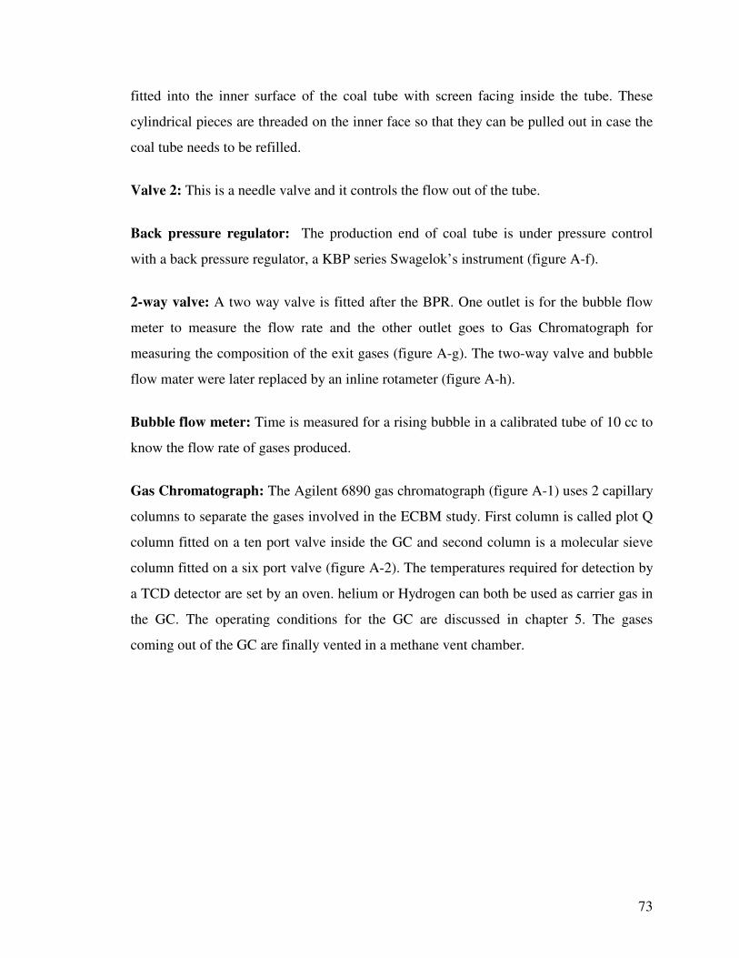
73
fitted into the inner surface of the coal tube with screen facing inside the tube. These
cylindrical pieces are threaded on the inner face so that they can be pulled out in case the
coal tube needs to be refilled.
Valve 2: This is a needle valve and it controls the flow out of the tube.
Back pressure regulator: The production end of coal tube is under pressure control
with a back pressure regulator, a KBP series Swagelok’s instrument (figure A-f).
2-way valve: A two way valve is fitted after the BPR. One outlet is for the bubble flow
meter to measure the flow rate and the other outlet goes to Gas Chromatograph for
measuring the composition of the exit gases (figure A-g). The two-way valve and bubble
flow mater were later replaced by an inline rotameter (figure A-h).
Bubble flow meter: Time is measured for a rising bubble in a calibrated tube of 10 cc to
know the flow rate of gases produced.
Gas Chromatograph: The Agilent 6890 gas chromatograph (figure A-1) uses 2 capillary
columns to separate the gases involved in the ECBM study. First column is called plot Q
column fitted on a ten port valve inside the GC and second column is a molecular sieve
column fitted on a six port valve (figure A-2). The temperatures required for detection by
a TCD detector are set by an oven. helium or Hydrogen can both be used as carrier gas in
the GC. The operating conditions for the GC are discussed in chapter 5. The gases
coming out of the GC are finally vented in a methane vent chamber.

74
Figure A-1: Gas Chromatograph
Figure A-2: Schematic of the valve and column configuration inside the GC
The overall setup is shown in figure A-3.

75
Figure A-3: Overall setup for single phase experiments
For two phase experiments, there are a few minor changes in the setup as discussed
below:
Water pump: To saturate the tube with water, a high pressure water pump is used to
inject water at a constant rate. Back pressure of the coal tube is controlled which affects
the injection pressure of water in the tube. The injection is done from a calibrated glass
tube filled with water as shown in the figure so that material balance can be done for
water (figure A-j).
Water trap: A water trap is set after the BPR, before the mixture is passed into the
bubble flow meter and then in the GC. It’s a glass tube sealed at the top with a rubber
stopper with two holes in it. One hole lets in the mixture of gases and liquid coming out
of the coal tube. Water settles down in this glass tube and gas comes out through the other
hole to the flow meter and then to the GC. The tube is kept inside an ice pack which helps
in condensing all the water (figure A-i).

76
Figure A: The different pieces of the experimental setup

77
Appendix B
B. Porosity Measurement Data
Total Volume of coal tube = 142.29 cc
Dead volume of the cylindrical bomb = 2.2 cc (measured by water injection)
Dead volume of the coal tube = 2.98 cc (measured by water injection)
Gas used for measuring porosity: Helium
Table B: Porosity measurement data
Set #
Initial Volume (cc)
Final Volume (cc)
Initial Pressure
(Psia)
Final pressure
(psia)
Pore Volume (cc)
Porosity
V1 VT P1 PT Vpore �
1 152.2 221.77 51 35 66.59 0.46
2 152.2 215.1 53 37.5 59.92 0.42
3 152.2 216.69 42 29.5 61.51 0.43
4 152.2 218.9 105 73 63.72 0.44
5 152.2 214.36 100 71 59.18 0.42

78
Appendix C
C. Permeability Measurement Data
Length of the coal tube, l = 302 cm
Area of cross section of the coal tube, A = 0.4711 cm2
Viscosity of helium, � = 0.018 cp
Table C: Permeability measurement data
Set #
Injection Pressure
(psia)
Exit Pressure
(psia)
Pressure drop (psia)
Exit flow rate
(cc/min)
Permeability (md)
Pinj Pexit �P q k
1 48 14.7 33.3 9.1 762.52
2 56 14.7 41.3 11.3 763.46

79
Appendix D
D. Simulation Data File
**--------------------------------------------------------------------** ** Dispersion_Test.DAT **--------------------------------------------------------------------** **--------------------------------------------------------------------** *RESULTS *SIMULATOR *GEM *FILENAMES *OUTPUT *SRFOUT *RESTARTOUT *INDEX-OUT *MAINRESULTSOUT *TITLE1 'ECBM Problem' *INUNIT *SI *DIM *MDIMPL 100 *WSRF *GRID 1 *WSRF *WELL 1 *WPRN *GRID *TIME *WPRN *WELL 1 *WRST 0 *OUTSRF *RES *ALL *OUTSRF *GRID *PRES *SW *SG *Y 'He' *Y 'N2' *DENW *DENG *VISG *ADS 'He' *ADS 'N2' *OUTPRN *RES *NONE *OUTPRN *GRID *NONE *OUTPRN *WELL *BRIEF **--------------------------------------------------RESERVOIR DATA *GRID *CART 90 1 1 *KDIR *DOWN *DUALPOR *DI *CON 0.033 *DJ *CON 0.007 *DK *CON 0.007 *PAYDEPTH *CON 1000.0 *DIFRAC *CON 0.000358 *DJFRAC *CON 0.000358 *DKFRAC *CON 0.000358 *POR *FRACTURE *CON 0.34 *POR *MATRIX *CON 0.10 *PERMI *FRACTURE *CON 760.0 *PERMJ *FRACTURE *CON 760.0

80
*PERMK *FRACTURE *CON 760.0 *PERMI *MATRIX *CON 10.0 *PERMJ *MATRIX *CON 10.0 *PERMK *MATRIX *CON 10.0 *CPOR *MATRIX 1.45E-7 *CPOR *FRACTURE 1.45E-7 *PRPOR *MATRIX 275.0 *PRPOR *FRACTURE 275.0 **--------------------------------------------------FLUID COMPONENT DATA ** PVT UNITS CONSISTENT WITH *INUNIT *SI *MODEL *PR *NC 2 2 *TRES 15.000 *PVC3 1.2000000E+00 *COMPNAME 'He' 'N2' *SG 1.4000000E-01 5.6000000E-01 *TB -2.6890000E+02 -1.9600000E+02 *PCRIT 2.2400000E+00 3.3940000E+01 *VCRIT 5.7300000E-02 9.0000000E-02 *TCRIT 5.0500000E+00 1.2620000E+02 *AC -0.390000E-00 0.4000000E-01 *MW 4.0000000E+00 2.8000000E+01 *HCFLAG 0 0 *BIN 1.000000E-01 *VSHIFT 0.0000000E+00 0.0000000E+00 *VISCOR *HZYT *MIXVC 1.0000000E+00 *VISVC 9.9000000E-02 9.0000000E-02 *VISCOEFF 1.0230000E-01 2.3364000E-02 5.8533000E-02 -4.0758000E-02 9.3324000E-03 *OMEGA 4.5723553E-01 4.5723553E-01 *OMEGB 7.7796074E-02 7.7796074E-02 *REFPW 101.325 *DENW 1000.0 *CW 5.8E-07 *VISW 1.0 **--------------------------------------------------ROCK FLUID---------- *ROCKFLUID *RPT 1 *SWT ** Sw Krw Krow

81
0 0 0.00001 0.4 0 *int 0.5 0.015 *int 0.525 0.02 *int 0.55 0.025 *int 0.575 0.04 *int 0.6 0.06 *int 0.65 0.1 *int 0.7 0.15 *int 0.75 0.225 *int 0.775 0.275 *int 0.8 0.31 *int 0.9 0.575 *int 1 1 0 *SLT ** Sl Krg Krog 0 1 0 0.4 1 *int 0.5 1 *int 0.525 0.975 *int 0.55 0.935 *int 0.575 0.82 *int 0.6 0.75 *int 0.65 0.47 *int 0.7 0.225 *int 0.75 0.08 *int 0.775 0.025 *int 0.8 0 *int 0.9 0 *int 1 0 0.00001 *RPT 2 *SGT 0.01 0 1 0 1 1 0 0 *SWT 0 0 1 0 1 1 0 0
*RTYPE *MATRIX *CON 1 *RTYPE *FRACTURE *CON 2 *ROCKDEN *MATRIX *CON 1466.0 *ROCKDEN *FRACTURE *CON 1466.0 *ADGMAXC 'He' *MATRIX *CON 0.001 ** gmol/kg of rock *ADGMAXC 'N2' *MATRIX *CON 0.227 ** gmol/kg of rock *ADGCSTC 'He' *MATRIX *CON 1.61E-04 ** 1/kPa *ADGCSTC 'N2' *MATRIX *CON 1.61E-04 ** 1/kPa *ADGMAXC 'He' *FRACTURE *CON 0.0

82
*ADGMAXC 'N2' *FRACTURE *CON 0.0 *ADGCSTC 'He' *FRACTURE *CON 1.61E-04 *ADGCSTC 'N2' *FRACTURE *CON 1.61E-04 *COAL-DIF-COMP 'N2' *CON 0 *COAL-DIF-COMP 'He' *CON 0 **--------------------------------------------------INITIAL CONDITION *INITIAL *VERTICAL *BLOCK_CENTER *WATER_OIL_GAS *NREGIONS 2 *REFPRES 482.5 482.5 *REFDEPTH 1000.0 1000.0 *DGOC 1500 1500 *DWOC 2000 2000 *SWOC 0.9999 0.9999 *ITYPE *FRACTURE *CON 1 *ITYPE *MATRIX *CON 2 *SEPARATOR 101.325 15.0 *ZGAS 1.0 0.0 1.0 0.0 **--------------------------------------------------NUMERICAL *NUMERICAL **--------------------------------------------------WELL DATA *RUN *DATE 2000 1 1 *AIMSET *FRACTURE *CON 3 *AIMSET *MATRIX *CON 3 *DTWELL 1.0E-6 *DTMIN 0.1E-6 *DTMAX 7.07E-5 *WELL 1 'PRODUCER' *PRODUCER 1 *OPERATE *MIN *BHP 480 *GEOMETRY *K 0.003 0.34 1 0.0 *PERF *SLIMTUBE 1 90 1 1 0.011 *WELL 2 'INJECTOR' *INJECTOR 2 *INCOMP *SOLVENT 0.0 1.0 *OPERATE *MAX *STG 0.0039 *OPERATE *MAX *BHP 689 *GEOMETRY *K 0.003 0.34 1 0.0 *PERF *SLIMTUBE 2 1 1 1 0.011 *TIME 0.02 *TIME 0.04166 *TIME 0.0625

83
*TIME 0.0833 *TIME 0.104 *TIME 0.125 *TIME 0.146 *STOP
Recommended