ISS
N02
49-6
399
ISR
NIN
RIA
/RR
--94
29--
FR+E
NG
RESEARCHREPORTN° 9429November 9, 2021
Project-Teams HiePACS andPleiade
Extension ofCorrespondence Analysisto multiway data-setsthrough High OrderSVD: a geometricframeworkOlivier Coulaud, Alain Franc, Martina Iannacito
arX
iv:2
111.
0434
3v1
[m
ath.
NA
] 8
Nov
202
1

RESEARCH CENTREBORDEAUX – SUD-OUEST
200 avenue de la Vieille Tour33405 Talence Cedex
Extension of Correspondence Analysis tomultiway data-sets through High Order SVD:
a geometric framework
Olivier Coulaud∗, Alain Franc†‡, Martina Iannacito∗
Project-Teams HiePACS and Pleiade
Research Report n° 9429 — November 9, 2021 — 20 pages
Abstract: This paper presents an extension of Correspondence Analysis (CA) to tensors throughHigh Order Singular Value Decomposition (HOSVD) from a geometric viewpoint. Correspondenceanalysis is a well-known tool, developed from principal component analysis, for studying contin-gency tables. Different algebraic extensions of CA to multi-way tables have been proposed overthe years, nevertheless neglecting its geometric meaning. Relying on the Tucker model and theHOSVD, we propose a direct way to associate with each tensor mode a point cloud. We provethat the point clouds are related to each other. Specifically using the CA metrics we show thatthe barycentric relation is still true in the tensor framework. Finally two data sets are used tounderline the advantages and the drawbacks of our strategy with respect to the classical matrixapproaches.
Key-words: Correspondence analysis, Tucker model, HOSVD, tensors, barycentric relation,point clouds
∗ HiePACS team, Inria Bordeaux-Sud-Ouest, France† BIOGECO, INRAE, Univ. Bordeaux, 33610 Cestas, France‡ Pleiade team - Inria\INRAE Bordeaux-Sud-Ouest, France
Extension de l’analyse des correspondances à des donnéeesmulti-dimensionnelles : un point de vue géométrique
Résumé : Ce document présente une extension de l’analyse des correspondances aux tenseurspar la décomposition en valeurs singulières d’ordre élevé (HOSVD) d’un point de vue géométrique.L’analyse des correspondances est un outil bien connu, développé à partir de l’analyse en com-posantes principales, pour étudier les tables de contingence. Différentes extensions algébriquesde l’analyse des correspondances aux tables à voies multiples ont été proposées au fil des ans. Ennous appuyant sur le modèle de Tucker et la HOSVD, nous proposons d’associer à chaque moded’un tenseur un nuage de points. Nous établissons un lien entre les cordonnées de ces différentsnuages. Une telle relation est classique en Analyse Factorielle des Correspondances (AFC) pourjustifier la projection simultanée des profils lignes et profils colonnes d’une table de contingence(d’où le nom de correspondance). Nous étendons une telle relation barycentrique aux liens entreles nuages de points associés aux différents modes de l’Analyse Factorielle des CorrespondancesMultiple d’un tenseur, construite via la HOSVD avec les métriques de l’AFC.
Mots-clés : Analyse des correspondances, modèle de Tucker, HOSVD, tenseurs, relationbarycentrique, nuages de points
Extension of CA to multiway data-sets through HOSVD 3
1 Introduction
Dimension reduction has been and still is one of the most widely used method to address modelingquestions on data sets living in large dimensional spaces [1, 2, with further detailed referenceswithin]. One of the most popular and used method is Principal Component Analysis (PCA) [3,4, 5, 6, 7, 8, 9, 10, 11]. It has three guises
1. an algebraic framework, working with vector spaces and matrix algebra, based on theSingular Value Decomposition (SVD) of the data matrix, see, e.g., [12]
2. a geometric framework, by associating a point cloud with the matrix representing the dataset (one point per row, one dimension per feature), see, e.g., [13, 14]
3. a statistical modeling approach, see, e.g., [15, 16].
PCA has been extended to a diversity of situations, like Correspondence Analysis (CA) [17,18, 19, 20, 21, 22, 23] for the analysis of contingency tables with metrics associated with χ2
distances [23, 24]. From an algebraic perspective, CA is the PCA of a contingency table withthe metric associated with the inverse of row and column marginals. CA has been explained ina geometric framework as well [25, 26]. Indeed, as for PCA, in the geometric view of CA eachrow of a contingency table corresponds to the coordinates of a point in a specific vector space.Since a similar argument holds for both rows and columns, a contingency table is naturallyassociated with a two point clouds. Thanks to the underlying dimension reduction techniques,CA makes possible the simultaneous visualization and interpretation of the two point clouds ina low dimension space where a specific barycentric relation links the two objects. The dictionarybetween the geometric and algebraic framework relies on the selection of weights and metrics inthe spaces where the point clouds live, see [13, 14].
Multiway data have appeared in a wide range of domains, requesting a further developmentof these analysis techniques. PCA and associated methods have been extended algebraically todimension reduction in multiway array, see, e.g., [27, 28, 29, 30, 31, 32, 33] and many referencestherein, with a link with tensor algebra [34]. These are algebraic extensions, relying on numericalcomputations based on elementary operations in tensor algebra in the same way that PCA andCA rely on numerical linear algebra. Starting from the generalization of PCA to multiway datathrough the Tucker model [35], with High Order Singular Value Decomposition (HOSVD) [30], analgebraic development of CA to MultiWay Correspondence Analysis (MWCA) follows naturally.Indeed MWCA is the HOSVD of a multiway contingency table associated with metric of themarginal inverse per each mode, see [29]. Our work aims to study the geometric perspectiveof MWCA, which is still poorly investigated. More precisely, we show that a point cloud isassociated with each mode of a tensor in MWCA in the same way that a point cloud is associatedwith either rows or columns of a matrix. Finally, the correspondence between two point cloudsbased on scaling and computing barycenters holding in the classical CA is generalized to d pointclouds in MWCA.
The remainder of this paper is organized as follows. Section 2 introduces all the prelim-inary tensor definitions, spaces and operations, clarifying the chosen notations. In Section 3the algebraic link between the principal components is presented. In particular, Subsection 3.3extends the results of the previous subsections in a space with generic metric. Section 4 presentsthe barycentric relation characterizing Correspondence Analysis in the tensor case. Finally wehighlight the different outcome on two data sets using the previous theoretical results.
RR n° 9429
4 Coulaud & Franc & Iannacito
2 Preliminaries
2.1 NotationsHere real numbers and integers are denoted by small Latin letters, vectors by boldface Latinletters, matrices by capital Latin letters and tensors by boldface capital Latin letters. O(m× n)denotes the set of all the real orthogonal matrices of m rows and n columns. Let us have d finitedimensional vector spaces E1, . . . , Ed on a same field R. Let A be a tensor in E1⊗ · · ·⊗Ed withdim Eµ = nµ for µ ∈ {1, . . . , d}. The integer d is called the order of the tensor A, each vectorspace Eµ is called a mode and nµ is the dimension of the tensor A for mode µ. We denote aswell A ∈ Rn1×···×nd . The matricization or unfolding of A with respect to the mode µ denotedby A(µ) is a matrix of nµ rows and n6=µ columns with n 6=µ =
∏α6=µ nα, see [30, Definition 1].
Notice that the matricization with respect to mode µ maps the (i1, . . . , id)-th tensor element tothe (iµ, i1, . . . , iµ−1, iµ+1, . . . , id)-th matrix element with
i1, . . . , iµ−1, iµ+1, . . . , id = 1 +
d∑α=1α 6=µ
(iα − 1)mα with mα =
α−1∏β=1β 6=µ
nβ , (1)
see [33]. Finding an approximation of Tucker model is facilitated by using an elementary op-erations on tensors: the Tensor-Times-Matrix product (TTM). Let A ∈ E1 ⊗ · · · ⊗ Ed, andMµ ∈ L(Eµ, Eµ) ' Eµ ⊗ Eµ for any mode µ. Let A be an elementary tensor A = a1 ⊗ · · · ⊗ adwith aµ ∈ Eµ. Then, TTM product of (M1, . . . ,Md) with A, denoted (M1, . . . ,Md)A, is thetensor M1a1 ⊗ · · · ⊗Mdad. This is extended to any tensor by linearity, see, e.g., [30]. Let A bea tensor of E1⊗ · · · ⊗Ed and let (M1, . . . ,Md) be a d-tuple of matrices of compatible dimensionwith A. If B = (M1, . . . ,Md)A, then the µ-matricization of B is
B(µ) = MµA(µ)(Md ⊗K · · · ⊗K Mµ+1 ⊗K Mµ−1 ⊗K · · · ⊗K M1)T (2)
for every µ ∈ {1, . . . , d} and, ⊗K the Kronecker product, we refer to [36, Proposition 3.7] forfurther details.
Let Nµ = M2µ be a Symmetric Positive Definite (SPD) matrix defining an inner product
on Eµ by 〈a,a′〉Mµ = 〈Mµa,Mµa′〉 = 〈Nµa,a′〉 = 〈a, Nµa′〉. It is extended to the whole
spaces by linearity. This induces an inner product on E1 ⊗ · · · ⊗ Ed on elementary tensors by〈a1⊗· · ·⊗ad , a
′1⊗· · ·⊗a′d〉m1⊗···⊗md = 〈M1a1⊗· · ·⊗Mdad , M1a
′1⊗· · ·⊗Mda
′d〉. Let us denote
by S = (⊗
µEµ,⊗
µ Iµ) the tensor space E1 ⊗ · · · ⊗ Ed endowed with standard inner productwith Iµ being the identity matrix on Eµ, and by Sm = (
⊗µEµ,
⊗µMµ) the same tensor space
when endowed with inner product induced by the matricesMµ. We will use the observation thatthe map
ν : Sm → S with ν(⊗µ
aµ)
=⊗µ
Mµaµ
is an isometry, because ‖⊗
µMµaµ‖ =∏µ ‖Mµaµ‖ =
∏µ ‖aµ‖mµ = ‖
⊗µ aµ‖m1⊗···⊗md where
‖ · ‖ denotes the Frobenius norm. This can be extended to the whole tensor space E1 ⊗ · · · ⊗Edby linearity (see [29] for details). The isometry can be written as ν(A) = (M1, . . . ,Md)A.
2.2 Tucker modelThe Tucker decomposition [35, 27, 37, 32, 33] of tensor A ∈ E1 ⊗ · · · ⊗ Ed is
A =
r1∑i1=1
· · ·rd∑id=1
Ci1...id u1i1 ⊗ · · · ⊗ udid (3)
Inria
Extension of CA to multiway data-sets through HOSVD 5
where the array of the (Ci1...id)i1,...,id is the core tensor of A and (uµiµ)iµ is an orthonormalbasis of Uµ ⊆ Eµ with rµ minimal for iµ ∈ {1, . . . , rµ} and µ ∈ {1, . . . , d}. So if A belongs toU1 ⊗ · · · ⊗ Ud with Uµ ⊆ Eµ and dimUµ = rµ, then r = (r1, . . . , rd) is the multilinear rank ofA [30]. In a synthetic way Tucker model is expressed with the TTM product asT = (U1, . . . Ud)C.We identify each Tucker subspace with its orthonormal basis, denoting Uµ ∈ O(nµ×rµ) for everymode µ ∈ {1, . . . , d}.
Starting from this Tucker model, we formulate an approximation problem as follows. Givena tensor A, its best Tucker approximation at multilinear rank r is the tensor T of multi-linearrank r such that ‖A−T‖ is minimal. This is a natural extension of PCA because the unknownsare the spaces (Uµ)µ under constraints of dimensions. Historically speaking, finding a solutionto Tucker best approximation has a long history which can be found, e.g., in [35, 29, 33, 38].There is no known algorithm yielding the best solution of the approximation problem, althoughseveral algorithms provide good quality results, known nowadays as High Order Singular ValueDecomposition (HOSVD) [30], its Truncated version (T-HOSVD) [39] and High Order Orthog-onal Iterations (HOOI) [31, 33]. The seminal paper for what is now called HOOI has beenpublished as Tuckals3 for 3-order tensors is [40] (see as well [32]). The extension to four modetensors has been made by Lastovicka in [41], and more generally to d-order multi-arrays by agroup in Groningen in 1986 [37]. These works used Kronecker product as an algebraic frame-work, and those results have been put into a common framework of tensor algebra in [29]. Bothapproaches (decomposition and best approximation) have been popularized by two papers by deLauthauwer et al. in 2000, who derived HOSVD [30] and HOOI [31] relying on matricizationand matrix algebra. Matricization, called unfolding as well, is building a matrix with one modein row, and a combination of the remaining ones in columns.
2.3 Multiway correspondence analysis
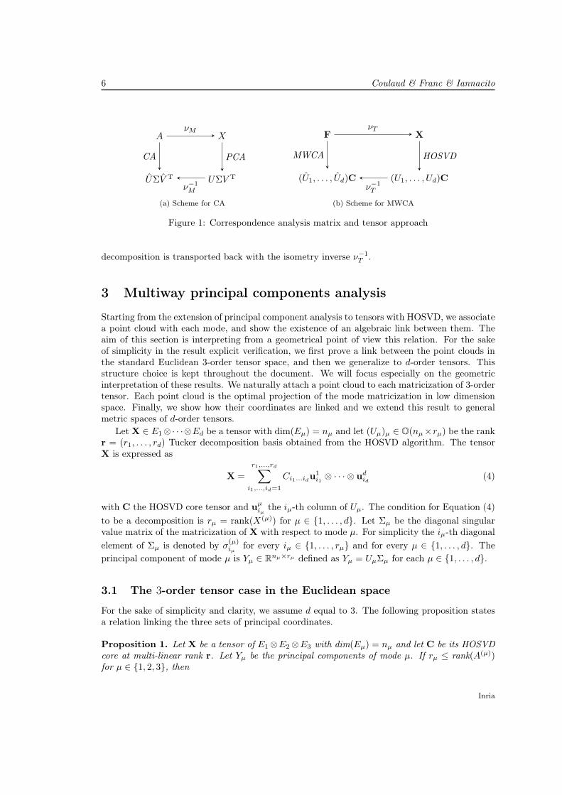
PCA is solving dimension reduction problem for a matrix in E ⊗ F , with E = Rm and F = Rnas natural choice in data science. In the geometric context, a cloud A of m points in Rn isassociated with a matrix A, where point i is row i of A (points are in F ). PCA of A is buildinga new orthonormal basis in F , called principal axis, and computing the coordinates of the pointsin this new basis, called principal components. Classically PCA is realized with a SVD of thegiven matrix, i.e., A = UΣV T. Then the principal axis are defined as the columns of V , andthe array of coordinates is given by Y = UΣ. It can be developed mutatis mutandis by selectingsome inner products associated with SPD matrices in E and/or F . Often in data analysis, thoseSPD matrices are diagonal, and the metrics are defined by weights. Indeed given M in Rm×mand Q in Rn×n, we define the inner product 〈A,B〉M⊗Q = 〈MAQ,MBQ〉. Then, PCA of A atrank r with this inner product is finding a rank r matrix Ar ∈ Rm×n such that ‖A−Ar‖M⊗Q isminimal. In other words, we compute the SVD at rank r of X = νM (A) = MAQ. If (Y,Λ, V ) isthe set of principal components Y of X, eigenvalues Λ = Σ2 and principal axis V , then, principalcomponents and axis of PCA of A with metrics so defined are (M−1Y,Λ, Q−1V ). In particular,as Figure 1a shows, CA is a PCA on a contingency table with metrics associated with inverse ofthe marginals as weights [13].
This is extended naturally to a multiway contingency table T [32], and formalized throughHOSVD. In Figure 1b we sketch this approach, which we call MWCA as it extends with HOSVDthe method of CA. As preprocessing step we compute the relative frequency tensor F dividingeach tensor T entry by the sum of all its entries. First step is to compute all marginals of F forall indices for all modes. This yields a vector of weights wµ = (wµi1 , . . . , w
µiµ
) for mode µ. In thesecond step the isometry νT is defined by the diagonal matrix Mµ whose diagonal elements areinverse of the weights. Third step is to perform HOSVD of X = νT (F). Finally the HOSVD
RR n° 9429
6 Coulaud & Franc & Iannacito
A X
UΣV T UΣV T
νM
PCA
ν−1M
CA
(a) Scheme for CA
F X
(U1, . . . , Ud)C (U1, . . . , Ud)C
νT
HOSVD
ν−1T
MWCA
(b) Scheme for MWCA
Figure 1: Correspondence analysis matrix and tensor approach
decomposition is transported back with the isometry inverse ν−1T .
3 Multiway principal components analysis
Starting from the extension of principal component analysis to tensors with HOSVD, we associatea point cloud with each mode, and show the existence of an algebraic link between them. Theaim of this section is interpreting from a geometrical point of view this relation. For the sakeof simplicity in the result explicit verification, we first prove a link between the point clouds inthe standard Euclidean 3-order tensor space, and then we generalize to d-order tensors. Thisstructure choice is kept throughout the document. We will focus especially on the geometricinterpretation of these results. We naturally attach a point cloud to each matricization of 3-ordertensor. Each point cloud is the optimal projection of the mode matricization in low dimensionspace. Finally, we show how their coordinates are linked and we extend this result to generalmetric spaces of d-order tensors.
Let X ∈ E1⊗· · ·⊗Ed be a tensor with dim(Eµ) = nµ and let (Uµ)µ ∈ O(nµ×rµ) be the rankr = (r1, . . . , rd) Tucker decomposition basis obtained from the HOSVD algorithm. The tensorX is expressed as
X =
r1,...,rd∑i1,...,id=1
Ci1...idu1i1 ⊗ · · · ⊗ udid (4)
with C the HOSVD core tensor and uµiµ the iµ-th column of Uµ. The condition for Equation (4)to be a decomposition is rµ = rank(X(µ)) for µ ∈ {1, . . . , d}. Let Σµ be the diagonal singularvalue matrix of the matricization of X with respect to mode µ. For simplicity the iµ-th diagonalelement of Σµ is denoted by σ(µ)
iµfor every iµ ∈ {1, . . . , rµ} and for every µ ∈ {1, . . . , d}. The
principal component of mode µ is Yµ ∈ Rnµ×rµ defined as Yµ = UµΣµ for each µ ∈ {1, . . . , d}.
3.1 The 3-order tensor case in the Euclidean space
For the sake of simplicity and clarity, we assume d equal to 3. The following proposition statesa relation linking the three sets of principal coordinates.
Proposition 1. Let X be a tensor of E1⊗E2⊗E3 with dim(Eµ) = nµ and let C be its HOSVDcore at multi-linear rank r. Let Yµ be the principal components of mode µ. If rµ ≤ rank(A(µ))for µ ∈ {1, 2, 3}, then
Inria
Extension of CA to multiway data-sets through HOSVD 7
Y1 = X(1)(Y3 ⊗K Y2)(B(1))T
Y2 = X(2)(Y3 ⊗K Y1)(B(2))T
Y3 = X(3)(Y2 ⊗K Y1)(B(3))T
with B = (Σ−11 ,Σ−12 ,Σ−13 )C.
Proof: We start the proof for the first mode principal components. Let X be expressed in theHOSVD basis as in Equation (4), i.e.,
X =
r1,r2,r3∑i,j,k=1
Cijku1i ⊗ u2
j ⊗ u3k.
Then the matricization of X with respect to mode 1 in the Tucker basis is expressed with theKronecker product as
X(1) =
r1∑i=1
u1i ⊗
( r2,r3∑j,k=1
Cijku3k ⊗K u2
j
). (5)
The PCA of X(1) is
X(1) = Y1VT1 =
r1∑i=1
σ(1)i u1
i ⊗ v1i (6)
with v1i the i-th column of V1 ∈ O(n2n3 × r1) and σ
(1)i u1
i i-th column of Y1 ∈ Rn1×r1 . Bycomparing Equations (5) and (6) for a fixed index i, we get
σ(1)i u1
i ⊗ v1i = u1
i ⊗( r2,r3∑j,k=1
Cijku3k ⊗K u2
j
).
Remarking that Σ1 is invertible, we identify v1i with a linear combination of the Kronecker
product of u2j and u3
k scaled by σ(1)i as
v1i =
1
σ(1)i
r2,r3∑j,k=1
Cijku3k ⊗K u2
j . (7)
Notice that the j-th and k-th column of Y2 = U2Σ2 and Y3 = U3Σ3 are σ(2)j u2
j and σ(3)k u3
k
respectively. So introducing in Equation (7) the singular values σ(2)j and σ
(3)k , we express the
i-th column of V1 as a linear combination of the Kronecker product of the j-th and k-th columnof Y2 and Y3, i.e.
v1i =
1
σ(1)i
r2,r3∑j,k=1
Cijkσ(2)j σ
(3)k
σ(2)j σ
(3)k
u3k ⊗K u2
j
=
r2,r3∑j,k=1
Cijk
σ(1)i σ
(2)j σ
(3)k
y3k ⊗K y2
j
=
r2,r3∑j,k=1
Bijk y3k ⊗K y2
jRR n° 9429
8 Coulaud & Franc & Iannacito
with B = (Σ−11 ,Σ−12 ,Σ−13 )C, y2j and y3
k the j-th and k-th column of Y2 and Y3 respectively .Remark that Y3⊗Y2 is a matrix of n2n3 rows and r2r3 columns whose `-th column is y3
k ⊗K y2j
with ` = jk for every j ∈ {1, . . . , r2}, k ∈ {1, . . . , r3} and ` ∈ {1, . . . , r2r3}, as defined inEquation (1). The tensor B matricized with respect to mode 1 is a matrix of r1 rows and r2r3columns, whose (i, jk)-th element is bijk for all j ∈ {1, . . . , r2}, k ∈ {1, . . . , r3}. So the sum inthe right-hand side of Equation (3.1) can be expressed as the matrix-product between Y3 ⊗K Y2and tensor B matricized with respect to mode 1 as
V1 = (Y3 ⊗K Y2)(B(1))T. (8)
Multiplying Equation (6) on the right by V1 yields Y1 = X(1)V1. Therefore multiplyingEquation (8) by the matricization of X with respect to mode 1, the principal component Y1 isexpressed as linear combination of the Kronecker product of principal components Y2 and Y3,i.e.
Y1 = X(1)V1 = X(1)(Y3 ⊗K Y2)(B(1))T.
The other relations follow straightforwardly from this one, permuting the indices coherently.
From an algebraic view this first proposition shows that the principal components of eachmode can be expressed as a linear combination of the principal components of the two othermodes. However as pointed out in the preliminary section, principal components can be seenfrom different viewpoints.
From a geometric viewpoint a point cloud Xµ is attached to each mode µ matricization oftensor X for µ ∈ {1, 2, 3}. Indeed the iµ-th row of X(µ) represents the coordinates of the iµ-thelement of mode µ point cloud living in the space Rn 6=µ where n 6=µ = n1n2n3
nµ. Given a multi-linear
rank r, we reformulate the problem of the Tucker approximation as a problem of dimensionalreduction. Indeed we look for the subspace of Rn6=µ of dimension rµ which minimizes in normthe projection of point cloud Xµ on it. This problem is solved with the HOSVD algorithm,which provides three orthogonal basis (U1, U2, U3) of the corresponding subspaces. Therefore theiµ-th row of Yµ = UµΣµ represents the coordinates of the iµ-th element of Xµ projected intothe subspace of Rn 6=µ of dimension riµ for µ ∈ {1, 2, 3}. The Proposition 1 result is interpretedgeometrically as each point cloud living in the linear subspace built from the Kronecker productof the other two.
3.2 Generalization to d-order tensorsNow, we generalize Proposition 1 to the d-case as follows.
Proposition 2. Let X be a tensor of E1⊗· · ·⊗Ed with dim(Eµ) = nµ and let C be its HOSVDcore at multi-linear rank r. Let Yµ be the principal components of mode µ. If rµ ≤ rank(A(µ))for µ ∈ {1, . . . , d}, then
Yµ = X(µ)(Yd ⊗K · · · ⊗K Yµ+1 ⊗K Yµ−1 ⊗K · · · ⊗K Y1)(B(µ))T
with B = (Σ−11 , . . . ,Σ−1d )C for every µ ∈ {1, . . . , d}.
Proof: The proof is very similar to that of Proposition 1, so we give only the main steps. Letstart by the first mode principal components. The 1-mode matricization of X in the Tucker basisis expressed with the Kronecker product, getting
X(1) =
r1∑i1=1
u1i1 ⊗
( r2,...,rd∑i2,...,id=1
Ci1...idudid⊗K · · · ⊗K u2
i2
). (9)
Inria
Extension of CA to multiway data-sets through HOSVD 9
The PCA of X(1) leads to
X(1) = Y1VT1 =
r1∑i1=1
σ(1)i1
u1i1 ⊗ v1
i1 (10)
with v1i1
the i1-th unitary column of V1 ∈ O(n 6=1 × r1) where n 6=1 =∏dµ=2 nµ and σ(1)
i1u1i1
thei1-th column of Y1 ∈ Rn1×r1 . Comparing Equations (9) and (10) for a fixed index i1, we identifyv1i1
with a linear combination of the Kronecker product of uµiµ for µ ∈ {2, . . . , d} scaled by σ(1)i1
as
v1i1 =
1
σ(1)i1
r2,...,rd∑i2,...,id=1
Ci1...idudid⊗K · · · ⊗K u2
i2 . (11)
Introducing in Equation (11) the singular values σ(µ)iµ
, we express the i1-th column of V1 as alinear combination of the Kronecker product of the iµ-th column of Yµ for every iµ ∈ {2, . . . , d}as
v1i1 =
r2,...,rd∑i2,...,id=1
Ci1...id
σ(1)i1σ(2)i2. . . σ
(d)id
σ(2)i2. . . σ
(d)id
udid ⊗K · · · ⊗K u2i2
=
r2,...,rd∑i2,...,id=1
Bi1...id ydid⊗K · · · ⊗K y2
i2
(12)
with B = (Σ−11 , . . . ,Σ−1d )C and yµiµ the iµ-th column of Yµ for µ ∈ {2, . . . , d}. Thanks to thecorrespondence between Kronecker product and matricization, the right-hand-side of Equation(12) is expressed as the matrix-product between Yd ⊗K · · · ⊗K Y2 and tensor B matricized withrespect to mode 1 and transposed as
V1 = (Yd ⊗K · · · ⊗K Y2)(B(1))T. (13)
Multiplying Equation (10) on the right by V1 yields Y1 = X(1)V1 and replacing V1 by its expres-sion of Equation (13), it finally follows
Y1 = X(1)V1 = X(1)(Yd ⊗K · · · ⊗K Y2)(B(1))T.
The other relations follow straightforwardly from this one, permuting the indices coherently.
3.3 Extension to generic metric space for d-order tensorsAs discussed in Section 2, the minimization problem faced with the HOSVD algorithm is ex-pressed by the Frobenious norm, induced by an inner product. The standard inner product isdefined by the identity matrix. However, whatever SPD matrix induces an inner product andthe associated metric norm on a vector space, which is therefore isomorphic to the standard Eu-clidean space. We emphasize in this section the role of the metric on the relationships betweenpoint clouds, using this isomorphic relationship between Euclidean spaces with different innerproducts.
Let F ∈ SM where SM is the tensor space E1 ⊗ · · · ⊗ Ed with dim(Eµ) = nµ endowed withthe inner product induced by SPD matrices Mµ of size nµ. Let S be the Euclidean tensor spaceE1 ⊗ · · · ⊗ Ed endowed with the standard inner product. As already mentioned, we can moveback to S, thanks to the isometry define as ν : SM → S, such that X = ν(F) = (M1, . . . ,Md)F.Let now X ∈ S be the HOSVD approximation of ν(F) at multi-linear rank r and let (Uµ)µ ∈
RR n° 9429
10 Coulaud & Franc & Iannacito
O(nµ×rµ) be the associated basis. Σµ is the singular value matrix of X(µ) and define Yµ = UµΣµthe principal components of mode µ for tensor X for every µ ∈ {1, . . . , d}. Let Wµ = M−1µ Yµ bethe principal components of F in the tensor space SM . In the following proposition, we link thesets of principal components in the metric space SM . As previously, for the sake of clarity theresult is first proved for d = 3 and afterwards geralized to whatever order d.
Proposition 3. Let F be a tensor in SM and let X be its image through the isometry ν in thestandard tensor space S. Let C be the HOSVD core tensor of X at multi-linear rank r such thatrµ ≤ rank(X(µ)) for µ ∈ {1, 2, 3}. Then for Wµ the principal component of mode µ of F in themetric tensor space SM it holds
W1 = F (1)(M23W3 ⊗K M2
2W2)(B(1))T
W2 = F (2)(M23W3 ⊗K M2
1W1)(B(2))T
W3 = F (3)(M22W2 ⊗K M2
1W1)(B(3))T
with B = (Σ−11 ,Σ−12 ,Σ−13 )C.
Proof: This result comes straightforwardly from Proposition 1 proof by introducing the metricsmatrices. For completeness, we illustrate the proof focusing on the link for the principal compo-nents of the first mode. Let (Uµ)µ=1,2,3 be the HOSVD basis of X at multi-linear rank r withUµ ∈ O(nµ × rµ). Let Yµ = UµΣµ be the principal components of mode µ for tensor X, whereΣµ is the singular values matrix of X(µ). Proposition 1 yields
Y1 = X(1)(Y3 ⊗K Y2)(B(1))T (14)
with B = (Σ−11 ,Σ−12 ,Σ−13 )C. Notice that X = ν(F) = (M1,M2,M3)F. So thanks to Equa-tion (2), we express X(1) in function of F (1) as
X(1) = M1F(1)(MT
3 ⊗K MT2 )
and replacing it into (14), it gets
Y1 = M1F(1)(M3 ⊗K M2)(Y3 ⊗K Y2)(B(1))T (15)
since Mµ are SPD matrices. Remarking that Yµ = MµWµ from the Wµ definition, substitutingit in the Equation (15) we obtain
M1W1 = M1F(1)(M3 ⊗K M2)(M3W3 ⊗K M2W2)(B(1))T. (16)
Since M1 is SPD and consequently invertible, from the previous equation it follows the thesis.The other relations follow straightforwardly from this proof, permuting the indices coherently.
This result is easily generalized to d-order tensors as follows.
Proposition 4. Let F be a tensor in SM and let X be its image through the isometry ν in thestandard tensor space S. Let C be the HOSVD core tensor of X at multi-linear rank r such thatrµ ≤ rank(X(µ)) for for µ ∈ {1, . . . , d}. Then for Wµ the principal component of mode µ of F inthe metric tensor space SM it holds
Wµ = F (1)(M2dWd ⊗K · · · ⊗K M2
µ+1Wµ+1 ⊗K M2µ−1Wµ−1 ⊗K · · · ⊗K M2
1W1)(B(µ))T
with B = (Σ−11 , . . . ,Σ−1d )C for every µ ∈ {1, . . . , d}.
Proof: The proof is a direct consequence of Proposition 2 and Proposition 3, so the details areomitted here.
Inria
Extension of CA to multiway data-sets through HOSVD 11
4 Geometric view for multiway correspondence analysis
In this last section, we transport the previous results in the correspondence analysis framework.We firstly clarify the Euclidean space and its metric where we set our problem. Then we makeexplicit the point cloud relation in this particular context. As final outcome we are able to provethe correspondence between the point clouds attached to each mode.
In accordance with the correspondence analysis framework, we consider a d-way contingencytable T ∈ Nn1×···×nd . The first step for performing CA is scaling T by the sum of all itscomponents setting a new frequency tensor
F =1∑n1,...,nd
i1,...,id=1 Ti1...idT.
We first clarify the tensor space we will work with. Let fµ be the marginal of mode µ, i.e., thevector whose components are the sums of the slices in mode µ for all µ ∈ {1, . . . , d}. For examplethe i-th element of f1 is
f1i1 =
n2,...,nd∑i2,...,id=1
Fi1...id for all i1 ∈ {1, . . . , n1}.
We assume that fµ has no zero component and by construction fµiµ > 0 for every µ ∈ {1, . . . , d}.Let define Dµ = diag(
√fµ) ∈ Rnµ×nµ for each µ ∈ {1, . . . , d} and let assume that F belongs to
Rn1×···×nd endowed by the metric induced by the matrices (D−11 , . . . , D−1d ), since D−1µ is SPD forevery µ ∈ {1, . . . , d}. We denote by SM this metric space and by S the tensor space Rn1×···×nd
endowed with the standard inner product. Under this assumption, let ν the isometry betweenthe spaces SM and S and let X = ν(F) = (D−11 , . . . , D−1d )F. The general element of tensor X iswritten
Xi1...id =Fi1...id√f1i1 . . . f
did
.
Performing the HOSVD over tensor X at multi-linear rank r leads to a new orthogonal basis(Uµ)µ=1,...,d, to a core tensor C and to the principal components Yµ = UµΣµ for every µ ∈{1, . . . , d} in the standard tensor space. Focusing on the principal components Wµ = DµYµ oftensor F in SM , Proposition 4 entails
Wµ = F (1)(M2dWd ⊗K · · · ⊗K M2
µ+1Wµ+1 ⊗K M2µ−1Wµ−1 ⊗K · · · ⊗K M2
1W1)(B(µ))T
where B(µ) is the matricization of B = (Σ−11 , . . . ,Σ−1d )C for µ ∈ {1, . . . , d}. Let Zµ = D−2µ Wµ bethe principal components scaled by the singular value inverse for µ ∈ {1, . . . , d} in tensor spaceSM . Henceforth, we denote by zµiµ the iµ-th row of Zµ. Now we prove that each component ofvector zµiµ can be expressed as a scaling factor times the barycenter of the linear combinationsof the other two scaled principal component rows. We assume d equal to 3 to facilitate thecomprehension of the following proof.
Proposition 5. Let F be a tensor in the tensor space SM endowed with the norm induced by theinner product matrices Dµ = diag(
√fµ) with fµ the µ mode marginal of F for µ ∈ {1, 2, 3}. Let
Zµ ∈ Rnµ×rµ be the scaled principal components for tensor F of mode µ in SM . If rµ = rank(F (µ))
RR n° 9429
12 Coulaud & Franc & Iannacito
for every µ ∈ {1, 2, 3}, then
(z1i )` =1
σ1`
n2,n3∑j,k=1
r2,r3∑m,p=1
Fijkf1i
(z3k)p(z2j )m(B1)`mp
(z2j )m =1
σ2m
n1,n3∑i,k=1
r1,r3∑`,p=1
Fijkf2j
(z3k)p(z1i )`(B2)`mp
(z3k)p =1
σ3p
n1,n2∑i,j=1
r1,r2∑`,m=1
Fijkf3k
(z1i )`(z2j )m(B3)`mp
where Bµ = ΣµB(µ) from Proposition 3.
Proof: We describe the proof for the i-th row of Z1 with i ∈ {1, . . . , n1}. From Proposition 3,under the CA metric choice, it follows that the principal components of F in the tensor spaceSM satisfy the relation
W1 = F (1)(D−23 W3 ⊗K D−22 W2)(B(1))T = F (1)(Z3 ⊗K Z2)(B(1))T.
Multiplying on the left this last equation by D−21 , we obtain
Z1 = D−21 W1 = D−21 F (1)(Z3 ⊗K Z2)(B(1))T
and since B(1) = Σ−11 B(1)1 , it gets
Z1 = D−21 F (1)(Z3 ⊗K Z2)(Σ−11 B(1)1 )T. (17)
Making explicit the `-th component of z1i , the i-th row of Z1, from Equation (17), we have
(z1i )` = (Z1)i` =
n2,n3∑j,k=1
r2,r3∑m,p=1
(D−21 F (1))ijk(Z3 ⊗K Z2)jkmp(Σ−11 B
(1)1 )`mp
=
n2,n3∑j,k=1
r2,r3∑m,p=1
Fijkf1i
(Z3)kp(Z2)jm(B1)`mpσ1`
=1
σ1`
n2,n3∑j,k=1
r2,r3∑m,p=1
Fijkf1i
(z3k)p(z2j )m(B1)`mp
by the definition of z2j and z3k for every i ∈ {1, . . . , n1}, j ∈ {1, . . . , n2}, k ∈ {1, . . . , n3} and` ∈ {1, . . . , r1}. This final equation can be read as a mutual barycenter relation scaled by theinverse of the corresponding singular value. Indeed there is a list of weights terms which sum
to 1, i.e.,∑n2,n3
j,k=1
Fijkf1i
=f1i
f1i
= 1 times a linear combination expressed through B1 of z2j and z3k.
Moving back to the geometric perspective, the Proposition 5 states that the scaled coordinatesof a point cloud correspond to the barycenter of the other two point cloud scaled coordinates.
The two remaining barycentric relations follow from this proof, permuting coherently theindices.
Correspondence in CA refers to the correspondence of point cloud coordinates through thescaled barycentric relation. We proved that this well known relation in matrix framework is hold-ing also in the tensor one, through HOSVD. Therefore we propose to refer to it as correspondenceanalysis from HOSVD.
This final proposition is extended and verified straightforwardly for d-order tensors.
Inria
Extension of CA to multiway data-sets through HOSVD 13
Proposition 6. Let F be a tensor in the tensor space SM endowed with the norm inducedby the inner product matrices Dµ = diag(
√fµ) with fµ the µ mode marginal of F for every
µ ∈ {1, . . . , d}. Let Zµ ∈ Rnµ×rµ be the scaled principal components for tensor F of mode µ inSM . If rµ = rank(F (µ)) for µ ∈ {1, . . . , d}, then
(zµiµ)`µ =1
σµ`µ
d∑η=1η 6=µ
nη∑iη=1
rη∑`η=1
Fi1...idfµiµ
(zdid)`d · · · (zµ+1iµ+1
)`µ+1(zµ−1iµ−1
)`µ−1· · · (z2i2)`2(Bµ)`1...`d
where Bµ = ΣµB(µ) from Proposition 4.
Proof: From Proposition 4, under the CA metric choice, the 1st mode principal components ofF in SM are expressed as
W1 = F (1)(Zd ⊗K · · · ⊗K Z2)(B(1))T.
If the previous equation is multiplied by equation by D−21 and it has B(1) replaced by theequivalent Σ−11 B
(1)1 , it gets
Z1 = D−21 F (1)(Zd ⊗K · · · ⊗K Z2)(Σ−11 B(1)1 )T. (18)
Making explicit the `1-th component of z1i1 , the i1-th row of Z1, from Equation (18), it followsthe thesis, i.e.
(z1i1)`1 =1
σ1`1
n2,...,nd∑i2,...,id=1
r2,...,rd∑`2,...,`d=1
Fi1...idf1i1
(zdid)`d · · · (z2i2)`2(B1)`1...`d .
The proof for the other modes follows directly from this one permuting coherently the indices.
5 ApplicationsIn this section we compare the MWCA based on the point cloud relation proved in Section 4with the classical CA performed on the same data reorganized as a matrix. Indeed, if we assumeF ∈ Rn1×···×nd to store the data relative frequencies as a tensor, then their matrix representationis given by Ak, the mode k-matricization of F, once mode k has been selected. The MWCA isperformed on F, while CA is performed on Ak. Let denote by F (k) the k-matricization of F afterapplying the isometry, similarly Ak is the outcome of isometry in the CA case. Since the twoapproaches are different, the isometries transporting F and Ak differ and so do Ak and F (k). Toestimate this discrepancy between the two objects we define the relative error e(F (k), Ak)
e(F (k), Ak) =||F (k) − Ak||||F (k)||
. (19)
The SVD and HOSVD, over which CA and MWCA relay respectively, provide an orthogonalbasis for the matrix or the decomposed tensor, which is unique up to an orthogonal rotation. Asproposed in [42] and [43], we orient these new basis selecting as leading direction the one wherethe majority of the data points out. To perform CA and MWCA we used python 3.6.9 andthe library TensorLy 0.6.0, see [44].
We first analyse with these two techniques the data reported in [45]. This example is im-portant since it shows that the multiway method results are coherent with those stated withcorrespondence analysis. Then the multiway barycentric relation is used to interpret an originaldata-set from the ecological domain [46].
RR n° 9429
14 Coulaud & Franc & Iannacito
Males Females
Agegroup
Verygood Good Regular Bad Very
badVerygood Good Regular Bad Very
bad
16-24 145 402 84 5 3 98 387 83 13 3
25-34 112 414 74 13 2 108 395 90 22 4
35-44 80 331 82 24 4 67 327 99 17 4
45-54 54 231 102 22 6 36 238 134 28 10
55-64 30 219 119 53 12 23 195 187 53 18
65-74 18 125 110 35 4 26 142 174 63 16
+75 9 67 65 25 8 11 69 92 41 9
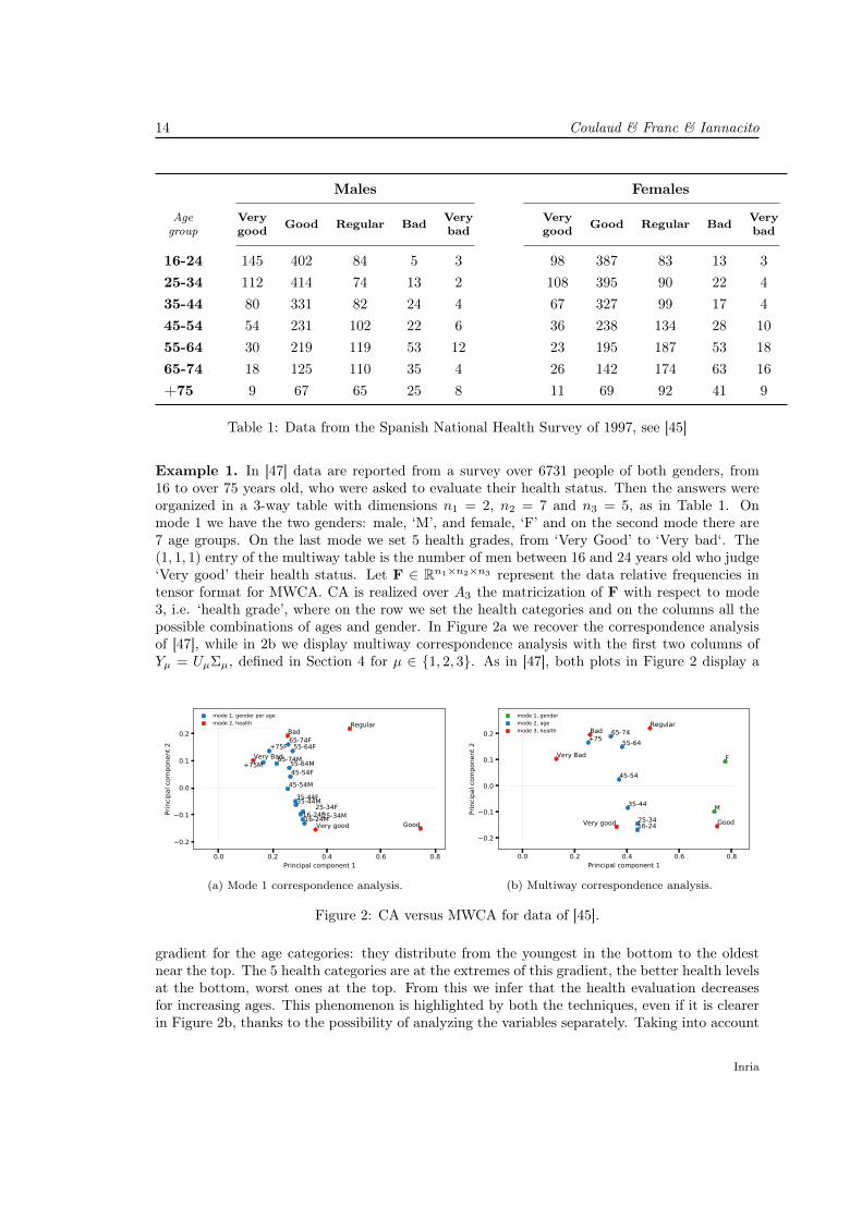
Table 1: Data from the Spanish National Health Survey of 1997, see [45]
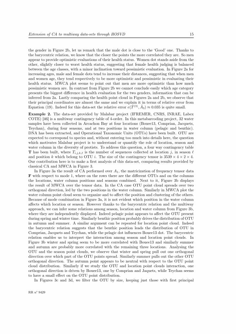
Example 1. In [47] data are reported from a survey over 6731 people of both genders, from16 to over 75 years old, who were asked to evaluate their health status. Then the answers wereorganized in a 3-way table with dimensions n1 = 2, n2 = 7 and n3 = 5, as in Table 1. Onmode 1 we have the two genders: male, ‘M’, and female, ‘F’ and on the second mode there are7 age groups. On the last mode we set 5 health grades, from ‘Very Good’ to ‘Very bad‘. The(1, 1, 1) entry of the multiway table is the number of men between 16 and 24 years old who judge‘Very good’ their health status. Let F ∈ Rn1×n2×n3 represent the data relative frequencies intensor format for MWCA. CA is realized over A3 the matricization of F with respect to mode3, i.e. ‘health grade’, where on the row we set the health categories and on the columns all thepossible combinations of ages and gender. In Figure 2a we recover the correspondence analysisof [47], while in 2b we display multiway correspondence analysis with the first two columns ofYµ = UµΣµ, defined in Section 4 for µ ∈ {1, 2, 3}. As in [47], both plots in Figure 2 display a
0.0 0.2 0.4 0.6 0.8Principal component 1
0.2
0.1
0.0
0.1
0.2
Prin
cipal
com
pone
nt 2
16-24M25-34M
35-44M
45-54M
55-64M65-74M+75M
16-24F25-34F
35-44F
45-54F
55-64F65-74F
+75F
Very good Good
RegularBad
Very Bad
mode 1, gender per agemode 2, health
(a) Mode 1 correspondence analysis.
0.0 0.2 0.4 0.6 0.8Principal component 1
0.2
0.1
0.0
0.1
0.2
Prin
cipal
com
pone
nt 2
M
F
16-2425-34
35-44
45-54
55-6465-74
+75
Very good Good
RegularBad
Very Bad
mode 1, gendermode 2, agemode 3, health
(b) Multiway correspondence analysis.
Figure 2: CA versus MWCA for data of [45].
gradient for the age categories: they distribute from the youngest in the bottom to the oldestnear the top. The 5 health categories are at the extremes of this gradient, the better health levelsat the bottom, worst ones at the top. From this we infer that the health evaluation decreasesfor increasing ages. This phenomenon is highlighted by both the techniques, even if it is clearerin Figure 2b, thanks to the possibility of analyzing the variables separately. Taking into account
Inria
Extension of CA to multiway data-sets through HOSVD 15
the gender in Figure 2b, let us remark that the male dot is close to the ‘Good’ one. Thanks tothe barycentric relation, we know that the closer the points the more correlated they are. So menappear to provide optimistic evaluations of their health status. Women dot stands aside from theother, slightly closer to worst health status, suggesting that female health judging is balancedbetween the age classes, with a minor inclination toward pessimistic evaluation. In Figure 2a forincreasing ages, male and female dots tend to increase their distances, suggesting that when menand women age, they tend respectively to be more optimistic and pessimistic in evaluating theirhealth status. MWCA plot seems to point out that men are more optimistic than how muchpessimistic women are. In contrast from Figure 2b we cannot conclude easily which age categorypresents the biggest difference in health evaluation for the two genders, information that can beinferred from 2a. Lastly comparing the health point cloud in Figures 2a and 2b, we observe thattheir principal coordinates are almost the same and we explain it in terms of relative error fromEquation (19). Indeed for this data-set the relative error e(T (3), A3) ≈ 0.035 is quite small.
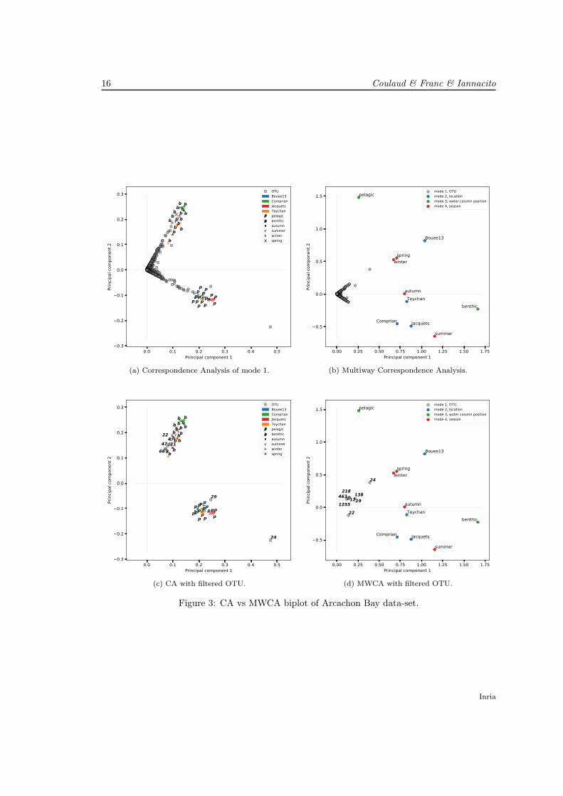
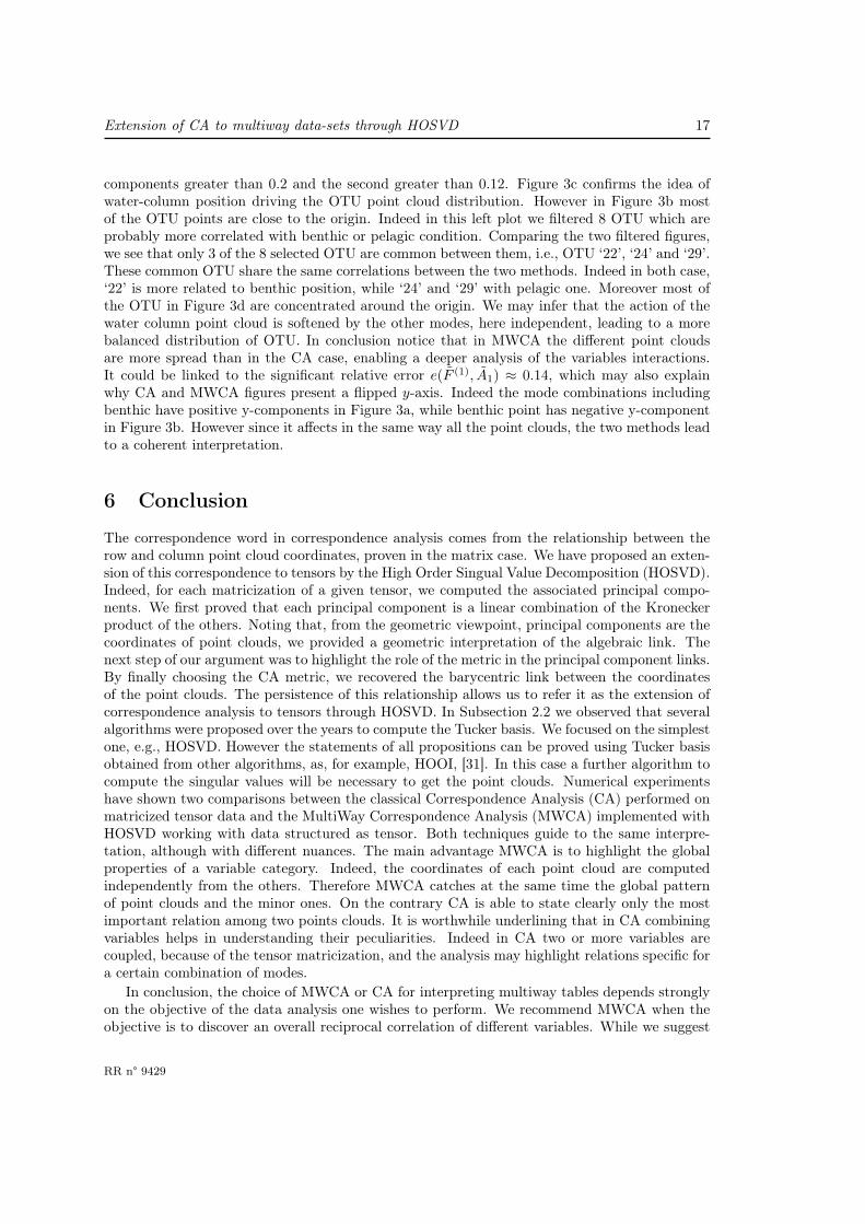
Example 2. The data-set provided by Malabar project (IFREMER, CNRS, INRAE, LabexCOTE) [46] is a multiway contingency table of 4-order. In this metabarcoding project, 32 watersamples have been collected in Arcachon Bay at four locations (Bouee13, Comprian, Jacquets,Teychan), during four seasons, and at two positions in water column (pelagic and benthic).DNA has been extracted, and Operational Taxonomic Units (OTUs) have been built. OTU areexpected to correspond to species and, without entering too much into details here, the questionwhich motivates Malabar project is to understand or quantify the role of location, season andwater column in the diversity of protists. To address this question, a four way contingency tableT has been built, where Ti,j,k,` is the number of sequences collected at location j, in season `and position k which belong to OTU i. The size of the contingency tensor is 3539 × 4 × 2 × 4.Our contribution here is to make a first analysis of this data-set, comparing results provided byclassical CA and MWCA in Figure 3.
In Figure 3a the result of CA performed over A1, the matricization of frequency tensor dataF with respect to mode 1, where on the rows there are the different OTUs and on the columnsthe locations, water column positions and seasons combined. Next to it, Figure 3b displaysthe result of MWCA over the tensor data. In the CA case OTU point cloud spreads over twoorthogonal direction, led by the two positions in the water column. Similarly in MWCA plot thewater column point cloud seem to organize and to affect the position and clustering of the others.Because of mode combination in Figure 3a, it is not evident which position in the water columnaffects which location or season. However thanks to the barycentric relation and the multiwayapproach, we can infer some relations among season, location and water column from Figure 3b,where they are independently displayed. Indeed pelagic point appears to affect the OTU presentduring spring and winter time. Similarly benthic position probably drives the distribution of OTUin autumn and summer. A similar argument can be repeated for location point cloud. Indeedthe barycentric relation suggests that the benthic position leads the distribution of OTU inComprian, Jacquets and Teychan, while the pelagic dot influences Bouee13 dot. The barycentricrelation enables us to interpret the interaction among season and location point clouds. InFigure 3b winter and spring seem to be more correlated with Bouee13 and similarly summerand autumn are probably more correlated with the remaining three locations. Analysing theOTU and the season point clouds, we observe that winter and spring pull out one orthogonaldirection over which part of the OTU points spread. Similarly summer pulls out the other OTUorthogonal direction. The autumn point appears to be neutral with respect to the OTU pointcloud distribution. Similarly if we study the OTU and location point clouds interaction, oneorthogonal direction is driven by Bouee13, one by Comprian and Jaquets, while Teychan seemsto have a small effect on the OTU point distribution.
In Figures 3c and 3d, we filter the OTU by size, keeping just those with first principal
RR n° 9429
16 Coulaud & Franc & Iannacito
0.0 0.1 0.2 0.3 0.4 0.5Principal component 1
0.3
0.2
0.1
0.0
0.1
0.2
0.3
Prin
cipal
com
pone
nt 2
pp
p p
b
b
b
b
pp p
p
bb
b b
pp p
p
b
b
bb
pp pp
b
b
b
b
OTUBouee13ComprianJacquetsTeychanpelagicbenthicautumnsummerwinterspring
(a) Correspondence Analysis of mode 1.
0.00 0.25 0.50 0.75 1.00 1.25 1.50 1.75Principal component 1
0.5
0.0
0.5
1.0
1.5
Prin
cipal
com
pone
nt 2
Bouee13
autumn
pelagic
Comprian
summer
benthic
Jacquets
winter
Teychan
spring
mode 1, OTUmode 2, locationmode 3, water column positionmode 4, season
(b) Multiway Correspondence Analysis.
0.0 0.1 0.2 0.3 0.4 0.5Principal component 1
0.3
0.2
0.1
0.0
0.1
0.2
0.3
Prin
cipal
com
pone
nt 2
4
821
22
24
29
4766
pp
p p
b
b
bb
pp p
p
b
bb
b
pp
pp
b
b
bb
pp p
p
bb
b
b
OTUBouee13ComprianJacquetsTeychanpelagicbenthicautumnsummerwinterspring
(c) CA with filtered OTU.
0.00 0.25 0.50 0.75 1.00 1.25 1.50 1.75Principal component 1
0.5
0.0
0.5
1.0
1.5
Prin
cipal
com
pone
nt 2
12
22
24
29138
218463
1255
Bouee13
autumn
pelagic
Comprian
summer
benthic
Jacquets
winter
Teychan
spring
mode 1, OTUmode 2, locationmode 3, water column positionmode 4, season
(d) MWCA with filtered OTU.
Figure 3: CA vs MWCA biplot of Arcachon Bay data-set.
Inria
Extension of CA to multiway data-sets through HOSVD 17
components greater than 0.2 and the second greater than 0.12. Figure 3c confirms the idea ofwater-column position driving the OTU point cloud distribution. However in Figure 3b mostof the OTU points are close to the origin. Indeed in this left plot we filtered 8 OTU which areprobably more correlated with benthic or pelagic condition. Comparing the two filtered figures,we see that only 3 of the 8 selected OTU are common between them, i.e., OTU ‘22’, ‘24’ and ‘29’.These common OTU share the same correlations between the two methods. Indeed in both case,‘22’ is more related to benthic position, while ‘24’ and ‘29’ with pelagic one. Moreover most ofthe OTU in Figure 3d are concentrated around the origin. We may infer that the action of thewater column point cloud is softened by the other modes, here independent, leading to a morebalanced distribution of OTU. In conclusion notice that in MWCA the different point cloudsare more spread than in the CA case, enabling a deeper analysis of the variables interactions.It could be linked to the significant relative error e(F (1), A1) ≈ 0.14, which may also explainwhy CA and MWCA figures present a flipped y-axis. Indeed the mode combinations includingbenthic have positive y-components in Figure 3a, while benthic point has negative y-componentin Figure 3b. However since it affects in the same way all the point clouds, the two methods leadto a coherent interpretation.
6 Conclusion
The correspondence word in correspondence analysis comes from the relationship between therow and column point cloud coordinates, proven in the matrix case. We have proposed an exten-sion of this correspondence to tensors by the High Order Singual Value Decomposition (HOSVD).Indeed, for each matricization of a given tensor, we computed the associated principal compo-nents. We first proved that each principal component is a linear combination of the Kroneckerproduct of the others. Noting that, from the geometric viewpoint, principal components are thecoordinates of point clouds, we provided a geometric interpretation of the algebraic link. Thenext step of our argument was to highlight the role of the metric in the principal component links.By finally choosing the CA metric, we recovered the barycentric link between the coordinatesof the point clouds. The persistence of this relationship allows us to refer it as the extension ofcorrespondence analysis to tensors through HOSVD. In Subsection 2.2 we observed that severalalgorithms were proposed over the years to compute the Tucker basis. We focused on the simplestone, e.g., HOSVD. However the statements of all propositions can be proved using Tucker basisobtained from other algorithms, as, for example, HOOI, [31]. In this case a further algorithm tocompute the singular values will be necessary to get the point clouds. Numerical experimentshave shown two comparisons between the classical Correspondence Analysis (CA) performed onmatricized tensor data and the MultiWay Correspondence Analysis (MWCA) implemented withHOSVD working with data structured as tensor. Both techniques guide to the same interpre-tation, although with different nuances. The main advantage MWCA is to highlight the globalproperties of a variable category. Indeed, the coordinates of each point cloud are computedindependently from the others. Therefore MWCA catches at the same time the global patternof point clouds and the minor ones. On the contrary CA is able to state clearly only the mostimportant relation among two points clouds. It is worthwhile underlining that in CA combiningvariables helps in understanding their peculiarities. Indeed in CA two or more variables arecoupled, because of the tensor matricization, and the analysis may highlight relations specific fora certain combination of modes.
In conclusion, the choice of MWCA or CA for interpreting multiway tables depends stronglyon the objective of the data analysis one wishes to perform. We recommend MWCA when theobjective is to discover an overall reciprocal correlation of different variables. While we suggest
RR n° 9429
18 Coulaud & Franc & Iannacito
the CA when the objective is to identify specific combination patterns.
7 Acknowledgments.The authors are very grateful to Luc Giraud for many helpful discussions and suggestions, whichhelped us improving this work. They thank also the teams of the Malabar project for sharingtheir data before their publication and letting them test their method.
References[1] A. J. Izenman, Modern Multivariate Statistical Techniques. NY: Springer, 2008.
[2] J. Wang, Geometric structure if high-dimensional data and dimensionality reduction.Springer, 2012.
[3] K. Pearson, “LIII. On lines and planes of closest fit to systems of points in space,” TheLondon, Edinburgh, and Dublin Philosophical Magazine and Journal of Science, vol. 2,no. 11, pp. 559–572, 1901.
[4] H. Hotelling, “Analysis of a complex of statistical variables into principal components.,”Journal of Educational Psychology, vol. 24, no. 6, pp. 417–441, 1933.
[5] K. R. Gabriel, “The biplot graphic display of matrices with application to principal compo-nent analysis,” Biometrika, vol. 58, pp. 453–467, 12 1971.
[6] W. Atchley and E. Bryant, Multivariate Statistical Methods: Among-Groups Covariation.Benchmark Papers in Systematic and Evolutionary Biology, Elsevier Science & TechnologyBooks, 1975.
[7] M. G. Kendall, Multivariate analysis. Griffin London, 1975.
[8] D. Morrison, D. Morrison, L. Marshall, M.-H. Incorporated, F. Morrison, H. Sahlin, N. Y. A.of Sciences, L. da Vinci Academy of Arts, and Sciences, Multivariate Statistical Methods.Annals of the New York Academy of Sciences, McGraw-Hill, 1976.
[9] J. Chambers, Computational Methods for Data Analysis. Wiley Series in Probability andMathematical Statistics, Wiley, 1977.
[10] I. T. Jolliffe, Principal Component Analysis. Springer Series in Statistics, Springer-VerlagNew York, second ed., 2002.
[11] I. T. Jolliffe and J. Cadima, “Principal component analysis: a review and recent devel-opments,” Philosophical Transactions of the Royal Society A: Mathematical, Physical andEngineering Sciences, vol. 374, no. 2065, p. 20150202, 2016.
[12] K. V. Mardia, J. Kent, and J. M. Bibby, Multivariate Analysis. Probability and Mathemat-ical Statistics, Academic Press, 1979.
[13] L. Lebart, A. Morineau, and J.-P. Fénelon, Traitement des données statistiques. Dunod,Paris, 1982.
[14] G. Saporta, Probabilités, Analyse de Données et Statistique. Editions Technip, 1990.
Inria
Extension of CA to multiway data-sets through HOSVD 19
[15] T. Anderson, An Introduction to Multivariate Statistical Analysis. Wiley Series in Proba-bility and Statistics, Wiley, 2003.
[16] C. R. Rao, Linear statistical Infernece and its Applications. Wiley Series in Probability andMathematical Statistics, Wiley, second ed., 1973.
[17] J. Benzécri and L. Bellier, L’analyse des données: Benzécri, J.-P. et al. L’analyse descorrespondances. L’analyse des données: leçons sur l’analyse factorielle et la reconnaissancedes formes, et travaux du Laboratoire de statistique de l’Université de Paris VI, Dunod,1973.
[18] M. O. Hill, “Correspondence analysis: A neglected multivariate method,” Journal of theRoyal Statistical Society: Series C (Applied Statistics), vol. 23, no. 3, pp. 340–354, 1974.
[19] M. Greenacre and L. Degos, “Correspondence analysis of HLA gene frequency data from124 population samples,” American journal of human genetics, vol. 29, pp. 60–75, 02 1977.
[20] M. J. Greenacre, “Some objective methods of graphical display of a data matrix,” SpecialReport). UNISA, Pretoria, 1978.
[21] H. G. Gauch, Multivariate Analysis in Community Ecology. Cambridge Studies in Ecology,Cambridge University Press, 1982.
[22] A. Gifi, Nonlinear Multivariate Analysis. Wiley Series in Probability and Statistics, Wiley,1990.
[23] M. J. Greenacre, Theory and Applications of Correspondence Analysis. Academic Press,1984.
[24] M. J. Greenacre, Correspondence Analysis in pratice. Chapman & Hall/CRC, second ed.,2007.
[25] B. Escofier-Cordier, L’analyse factorielle des correspondances. PhD thesis, University ofRennes, 1965.
[26] J. Benzécri, “Statistical analysis as a tool to make patterns emerge from data,” in Method-ologies of Pattern Recognition (S. Watanabe, ed.), pp. 35–74, Academic Press, 1969.
[27] P. M. Kroonenberg, Three-mode principal component analysis: Theory and applications.DSWO Press, Leiden, 1983.
[28] R. Coppi and S. Bolasco, eds., Multiway Data Analysis. North-Holland Publishing Co.,1989.
[29] A. Franc, Etude Algébrique des multitableaux: apports de l’algèbre tensorielle. PhD thesis,University of Montpellier, 1992.
[30] L. De Lathauwer, B. De Moor, and J. Vandewalle, “A multilinear singular value decompo-sition,” SIAM Journal on Matrix Analysis and Applications, vol. 21, no. 4, pp. 1253–1278,2000.
[31] L. De Lathauwer, B. De Moor, and J. Vandewalle, “On the best rank-1 and rank-(r1, r2, . . . , rn) approximation of high order tensors,” SIAM Journal on Matrix Analysisand Applications, vol. 21, no. 4, pp. 1324–1342, 2000.
RR n° 9429
20 Coulaud & Franc & Iannacito
[32] P. M. Kroonenberg, Applied Multiway Data Analysis. Wiley, 2008.
[33] T. G. Kolda and B. W. Bader, “Tensor decompositions and applications,” SIAM Review,vol. 51, pp. 455–500, September 2009.
[34] A. Franc, “Multiway arrays: some algebraic remarks,” in Multiway Data Analysis (R. Coppiand S. Bolasco, eds.), ch. 2, pp. 19–29, NLD: North-Holland Publishing Co., 1989.
[35] L. R. Tucker, “Some mathematical notes on three-modes factor analysis,” Psychometrika,vol. 31, no. 3, pp. 279–311, 1966.
[36] T. G. Kolda, “Multilinear operators for higher-order decompositions,” Tech. Rep.SAND2006-2081, Sandia National Laboratories, April 2006.
[37] K. Arie, H. Neudecker, and T. Wansbeek, “An approach to n−mode components analysis,”Psychometrika, vol. 51, no. 2, pp. 269–275, 1986.
[38] L. Grasedyck, “Hierarchical singular value decomposition of tensors,” SIAM Journal onMatrix Analysis and Applications, vol. 31, no. 4, pp. 2029–2054, 2010.
[39] N. Vannieuwenhoven, R. Vandebril, and K. Meerbergen, “A new truncation strategy for thehigher-order singular value decomposition,” SIAM Journal on Scientific Computing, vol. 34,no. 2, pp. A1027–A1052, 2012.
[40] P. Kroonenberg and J. de Leeuw, “Principal component analysis of three modes data bymeans of alternating least square algorithms,” Psychometrika, vol. 45, no. 1, pp. 69–97,1980.
[41] J. L. Lastovicka, “The extension of component analysis to four-mode matrices,” Psychome-trika, vol. 46, no. 1, pp. 47–57, 1981.
[42] R. Bro, E. Acar, and T. G. Kolda, “Resolving the sign ambiguity in the singular valuedecomposition,” Journal of Chemometrics, vol. 22, no. 2, pp. 135–140, 2008.
[43] R. Bro, R. Leardi, and L. G. Johnsen, “Solving the sign indeterminacy for multiway models,”Journal of Chemometrics, vol. 27, no. 3-4, pp. 70–75, 2013.
[44] J. Kossaifi, Y. Panagakis, A. Anandkumar, and M. Pantic, “Tensorly: Tensor learning inpython,” Journal of Machine Learning Research, vol. 20, no. 26, pp. 1–6, 2019.
[45] CARME-N, “Spanish national health survey.” http://www.carme-n.org/?sec=data2,2007. [Data-set 3].
[46] “Malabar project data paper (IFREMER, CNRS, INRAE, Labex COTE).” in prep., 202X.
[47] M. Greenacre, Correspondence Analysis in Practice. Academic Press, 1993. Data-sets areavailable at.
Inria

RESEARCH CENTREBORDEAUX – SUD-OUEST
200 avenue de la Vieille Tour33405 Talence Cedex
PublisherInriaDomaine de Voluceau - RocquencourtBP 105 - 78153 Le Chesnay Cedexinria.fr
ISSN 0249-6399
Recommended