
NCER Working Paper SeriesNCER Working Paper Series
Forecasting Spikes in Electricity Prices
T M ChristensenT M Christensen A S HurnA S Hurn K A LindsayK A Lindsay Working Paper #70Working Paper #70 January 2011January 2011
Forecasting Spikes in Electricity Prices
T M Christensen
Department of Economics, Yale University
A S Hurn
School of Economics and Finance, Queensland University of Technology
K A Lindsay
Department of Mathematics, University of Glasgow.
Abstract
In many electricity markets, retailers purchase electricity at an unregulated spot price andsell to consumers at a heavily regulated price. Consequently the occurrence of extrememovements in the spot price represents a major source of risk to retailers and the accu-rate forecasting of these extreme events or price spikes is an important aspect of effectiverisk management. Traditional approaches to modeling electricity prices are aimed primarilyat predicting the trajectory of spot prices. By contrast, this paper focuses exclusively onthe prediction of spikes in electricity prices. The time series of price spikes is treated asa realization of a discrete-time point process and a nonlinear variant of the autoregressiveconditional hazard (ACH) model is used to model this process. The model is estimated usinghalf-hourly data from the Australian electricity market for the sample period 1 March 2001to 30 June 2007. The estimated model is then used to provide one-step-ahead forecasts ofthe probability of an extreme event for every half hour for the forecast period, 1 July 2007to 30 September 2007, chosen to correspond to the duration of a typical forward contract.The forecasting performance of the model is then evaluated against a benchmark that isconsistent with the assumptions of commonly-used electricity pricing models.
KeywordsElectricity Prices, Price Spikes, Autoregressive Conditional Duration, AutoregressiveConditional Hazard, Electricity Futures.
JEL classification numbersC14, C52.
Corresponding authorStan HurnSchool of Economics and FinanceQueensland University of TechnologyBrisbane, Qld 4001Australia
email: [email protected]
1 Introduction
In the mid 1990s, the regional electricity markets of New South Wales, Queensland, Victoria,
South Australia, and the Australian Capital Territory were merged to form the National Elec-
tricity Market (NEM) in Australia.1 The NEM operates as a pooled market in which all available
supply to a region is aggregated and generators are dispatched so as to satisfy demand as cost
effectively as possible. If, in any given region, local demand exceeds local supply or electricity
in a neighbouring region is sufficiently inexpensive to warrant transmission, then electricity is
imported and exported between regions subject to the physical constraints of the transmission
infrastructure. In terms of composition of the supply side, coal-fired generators and hydroelectric
production have a low marginal cost of production supplying respectively 84% and 7.2% of the
NEM’s capacity. Gas turbines and oil-fired plants supply around 8.5% and 0.3% of the market,
respectively, and only take around 20 minutes to initiate generation but have a comparatively
high marginal cost of production, typically operating only during peak periods.
Wholesale trading in electricity is conducted as a spot market in which supply and demand are
instantaneously matched through a centrally-coordinated dispatch process. A summary of the
process for bidding, dispatch and calculation of the spot price is as follows. Prior to 12:30pm
on the day before production, generators bid their own supply curve, consisting of at most
ten price-quantity pairs for each half-hour of the following day, subject to a floor of -$1,000
and a ceiling of $10,000 per megawatt hour (MWh). Generators are free to re-bid quantities
but not prices up to approximately five minutes before dispatch. Upon receipt of bids from all
generators, the supply curves are aggregated and generators are dispatched in line with their
bids so that demand is satisfied as inexpensively as possible.2 The dispatch price for each five-
minute interval is the bid price of the marginal generator dispatched into production. The spot
price for each half-hour trading interval is then calculated as the arithmetic mean of the six
five-minute interval dispatch prices observed within the half-hour, and all transactions occurring
within the half-hour are settled at the spot price.3
Spot electricity prices are known to exhibit sudden and very large jumps to extreme levels, a
phenomenon usually attributed to unexpected increases in demand, unexpected shortfalls in
supply and failures of transmission infrastructure (Geman and Roncorni, 2006). The spikes re-
flect the fact that the central dispatch process needs to rely on the bids of the high marginal
1These markets were linked using large capacity transmission lines, with the exception of Queensland, whichparticipated under the NEM market rules but was not physically connected to the NEM until February 2001.
2For example, suppose Generator A bids 10,000MW at -$100/MWh and 5,000MW at $40/MWh and GeneratorB bids 5,000MW at $20/MWh. If the prevailing demand for the five minute period is 12,000MW, Generators Aand B will be dispatched to supply 10,000MW and 2,000MW respectively. The dispatch price will be $20/MWh.
3The NEM is therefore a continuous-trading market that is not be confused with day-ahead call markets whichoperate in some European markets, such as Germany, France and the Netherlands, in which prices are quotedfor delivery on each hour of the following day (see, for example, Huisman et al., 2007).
2
cost of production generators in order to satisfy demand. These extreme price events, or “price
spikes”, are particularly hazardous to electricity retailers who buy from the NEM at the spot
price and sell to consumers at a price that is heavily regulated (Anderson et al., 2006). Conse-
quently, improving the understanding of factors contributing to the occurrence of extreme price
events, as well as the accurate forecasting of these events, is crucial to effective risk management
in the retail energy sector. It is this forecasting problem that is the central concern of this paper.
Traditional approaches to modeling electricity prices fall, broadly speaking, into three categories
namely, traditional autoregressive time series models, nonlinear time series models with par-
ticular emphasis on Markov-Switching models and continuous-time diffusion or jump-diffusion
models.4 These models all share the common feature that they aim to characterize the trajectory
of the spot price or return across time.
Taken at face value, these models appear to differ in their treatment of price spikes. Traditional
autoregressive time-series models treat spikes through the use of thresholds (Misiorek et al.,
2006), Bernoulli and Poisson jump processes (Crespo Cuaresma et al., 2004; Knittel and Roberts,
2005) and a variety of heavy tailed error processes (Contreras et al., 2003; Bystrom, 2005; Garcia
et al., 2005; Swider and Weber, 2007; Panagiotelis and Smith, 2008). Markov-switching models
incorporate spikes by proposing different regimes, at least one of which is consistent with a state
of system stress in which a spike is more likely to occur (de Jong and Huisman, 2003; Huisman
and Mahieu, 2003; Weron et al., 2004; de Jong, 2006; Kosater and Mosler, 2006; Bierbrauer
et al., 2007; Becker et al., 2007). Diffusion models of the spot price introduce spikes through
the addition of a Poisson jump component with either a constant intensity parameter (Weron
et al., 2004; Cartea and Figueroa, 2005) or a time-varying intensity parameter (Escribano et
al., 2002; Knittel and Roberts, 2005) in which the intensity of the jump process is typically a
linear combination of deterministic seasonal and/or diurnal factors. Within the jump diffusion
approach, Chan, Gray and van Campen (2008) separate price volatility into jump and non-
jump components and then explore whether volatility forecasts can be improved by explicitly
incorporating the jump and non-jump components of the total variation.
All these models essentially regard price spikes as a memoryless process with intensity that
is independent of its history. There is evidence, however, to suggest that the intensity of the
spiking process is not homogeneous, nor is it driven by deterministic factors alone. Indeed,
there appears to be a significant historical component which is important in explaining the
intensity of the spiking process (Christensen et al., 2009). This paper complements the existing
econometric literature by focusing exclusively on forecasting extreme price events rather than
4Non-traditional approaches to forecasting price movements in electricity markets include artificial neuralnetworks or other data-mining techniques (see, for example, Zhao et al. (2007) and Xu and Nagasaka (2009)).Another approach is to focus on forecasting value-at-risk in electricity markets (Chan and Gray, 2006) ratherthan providing forecasts of the actual spot price.
3
on the trajectory of price. The sequence of such events is treated as a realization of a discrete
point process and an important characteristic of the econometric model is that it embeds the
information content of previous spikes. This dependence is achieved by way of a nonlinear
variant of the autoregressive conditional hazard (ACH) model originally developed by Hamilton
and Jorda (2002). Although the econometric model is developed and applied in the context
of a continuous-trading market, as it focuses on the forecasting of extreme events and not on
modeling the trajectory of electricity prices, it lends itself to adaption for treating extreme
events in day-ahead call markets as well.
The empirical work is implemented using data from four regions of the NEM. The ACH frame-
work permits simultaneous analysis of both the historical dependence of the spike rate, as well
as the influence of load and temperature factors. It is found that the occurrence of extreme
price events displays significant persistence and historical dependence even after taking load
and temperature factors into account. Additionally, spikes are found to be much more likely to
occur when load is comparatively high, as well as during times of extremes in temperature, in
accordance with the usual explanation for spikes outlined earlier. Importantly, the ACH model
is found to provide superior half-hour ahead forecasts of extreme price events by comparison
with forecasts made by an unconditional model that is broadly consistent with the type of
memoryless electricity-pricing model often employed in the literature. It should be noted that
price spikes are a generic feature of electricity markets worldwide (Escribano, et al., 2002) and
therefore the research reported here will be of general interest and applicability, notwithstanding
the fact that this paper is set within the Australian institutional framework.
The plan of the paper is as follows. Section 2 outlines the ACH framework, its relation to ACD
processes and its extension to capture nonlinearities in the duration process. Section 3 deals
with data and section 4 with estimation, and a discussion of the results. In section 5, half-hour
ahead forecasts of the ACH model are compared with forecasts made by a model consistent
with much of the electricity-pricing literature. Section 6 concludes.
2 The Econometric Model
The econometric model outlined in this section specifies the probability of observing an event as
a function of the history of a process and a set of exogenous variables. Additional factors con-
tributing to the severity of the observed event are also analyzed. The basic framework adopted
in this research is that proposed by Hamilton and Jorda (2002), modified following the work of
Engle and Dufour (2000) and Fernandes and Grammig (2006).
4
2.1 Autoregressive Conditional Duration
Prior to the development of the actual empirical model used in this paper, its historical an-
tecedents are reviewed briefly. Consider an orderly marked point process where events occur at
random times t0 < t1 < . . . < tn < . . ., with ti−1 representing the time at which the ith event
occurred. Let N(t) represent the number of events that have occurred in the interval (t0, t ] and
let Ht = {t0, t1, . . . , tN(t)|N(t)} represent the history of the process observed over [t0, t ]. The
conditional intensity function is defined as
λ(t |Ht) = lim∆t→0+
Prob(N(t+ ∆t) > N(t)|Ht)
∆t
so that
E[N(t+ ∆t) −N(t)|Ht] = λ(t |Ht)∆t+ o(∆) .
The econometric analysis of point processes typically deals with an appropriate parametrization
of λ with the aim of determining which exogenous variables, if any, drive the intensity of the pro-
cess and the extent to which this intensity is influenced by its history. In the absence of memory,
the process may be treated as a Poisson process with intensity dependent on exogenous vari-
ables alone. On the other hand, if the process exhibits memory, the modelling exercise becomes
more interesting because it must now address the additional question of how to incorporate the
history of the process (see, for example, Engle and Russell, 1998).
The autoregressive conditional duration (ACD) framework treats the conditional intensity of
the process as a function of the duration between previous events. Let uN(t) = tN(t) − tN(t)−1
represent the most recently observed duration between events. The conditional expectation of
the next duration, i.e. the elapsed time from the most recent event to the next event, is
ψN(t)+1 = E(uN(t)+1|Ht; θ) , (1)
where θ is a vector of parameters. The ACD model of Engle and Russell (1998) is then
ψN(t)+1 = uN(t)+1ǫN(t)+1 ,
in which the ǫ are i.i.d. non-negative random variables with unit mean. The conditional intensity
function is given by
λ(t |Ht) = λ0
(t− tN(t)
ψN(t)+1
)1
ψN(t)+1, (2)
in which λ0(·) is the quotient of the density function and survival function of ǫ.
A functional form for expression (1) and a distribution for the ǫ are required to fully specify the
ACD model. Arguably the simplest formulation is the exponential ACD model of order (p, q) in
which the ǫ are assumed to be i.i.d. exponentially-distributed random variables with unit mean
5
and where the durations are modelled as the ARMA(p, q) process
ψN(t)+1 = ω +
p∑
j=1
αjuN(t)+1−j +
q∑
j=1
βjψN(t)+1−j . (3)
Stationarity of the duration process requires that ω > 0, αj ≥ 0 for j = 1, . . . , p, βj ≥ 0 for
j = 1, . . . , q and∑p
j=1 αj +∑q
j=1 βj < 1. In terms of the model, the conditional expectation
of the next duration is updated as events occur. In particular, when events occur in quick
succession, the most recent lagged values of u are smaller, reducing the conditional expectation
of the next duration. Similarly when the duration between events is comparatively large, the
most recent lagged values of u are larger, increasing the conditional expectation of the next
duration. Taking ǫ as exponentially-distributed means that λ0 = 1 everywhere, so that the
expression for the conditional intensity in equation (2) becomes
λ(t|Ht) =1
ψN(t)+1.
This model has proved useful in the analysis of arrival times of stock trades (Engle and Russell,
1998; Engle, 2000) and foreign exchange trades (Engle and Russell, 1997). The basic ACD
model has been extended in numerous ways (see, for example, Bauwens and Giot, 2000; Engle
and Dufour, 2000; Zhang et al., 2001; Bauwens and Veredas, 2004; Feng et al., 2004; Engle and
Russell, 2005; Fernandes and Grammig, 2006).
2.2 Autoregressive Conditional Hazard
The ACD model and its variants share the common property that they aim to model the interval
between events when the underlying process is continuous in the sense that events can occur
at any instant in time. There are, however, many processes in economics and finance that are
fundamentally discrete, meaning that at most one event can occur within an interval of given
fixed duration. In the context of the modeling problem addressed by this research, namely the
incidence of price spikes in the Australian electricity market, the fixed interval of interest is
half an hour and all transactions within this fixed interval are settled at the pool price for that
interval. Consequently, spikes in the spot price of electricity provide one example of a situation
in which there is no duration to be modeled in the sense of the ACD model.
In respect of the incidence of price spikes in the electricity market, the appropriate question is
whether or not an event occurs in a given half hour. Consequently, it is necessary to think in
terms of conditional hazard, defined by
ht+1 = Prob(N(t+ 1) > N(t)|Ht) ,
which represents the probability of an event occurring in the given interval conditioned on Ht,
the past history of events now interpreted in terms of the discrete process. Consistency between
6
the continuous-time and discrete-time models requires the hazard of the discrete-time process
to be asymptotically equivalent to the intensity of the continuous-time process as the interval
length tends to zero. Hamilton and Jorda (2002) specify an autoregressive conditional hazard
(ACH) model which they demonstrate is the discrete-time equivalent of the ACD model. The
hazard function in this model is given by
ht+1 =1
ψN(t)+1, (4)
where ψN(t)+1 is defined in equation (3).
Consistency between the discrete and continuous models is maintained for a Box-Cox transfor-
mation of the observed and expected durations. This property allows a richer parameterization of
equation (3), similar to the Box-Cox ACD model introduced by Engle and Dufour (2000) which
itself is a subset of the general family of ACD models proposed by Fernandes and Grammig
(2006). In particular,
ψνN(t)+1 = ω∗ +
p∑
j=1
αjuνN(t)+1−j +
q∑
j=1
βjψνN(t)+1−j (5)
where ν > 0. Equation (5) nests the original ACH specification (ν = 1) and the ACH model in
log-durations, obtained in the limit as ν → 0+.
Equation (4) may be augmented to include the possible influence of a vector of exogenous
variables, zt+1, upon the conditional hazard by extending the specification of ht+1 to
ht+1 =1
Λ(exp(−γ′zt+1) + ψN(t)+1), (6)
where γ is a vector of coefficients and the function Λ is chosen to ensure that ht+1 represents a
probability. In this research, the link function proposed by Hamilton and Jorda (2002) is used,
who also suggest that the constant term may be omitted from the specification of ψN(t)+1, in
equation (3) or equivalently in equation (5), provided a constant term is included in zt+1 in
expression (6).
To summarize, the final model for the investigation of price spikes in the four regions of the
Australian electricity market comprises equations (5) and (6) with model parameters
θ = (γ, α1, . . . , αp, β1, . . . , βq, ν) ,
which are to be estimated from sample data. Let Xt take the value 1 if an event occurs in the
interval t and zero otherwise, then the conditional probability density function of Xt may be
written as
Prob(Xt = xt|Ht−1; θ) = hxt
t (1 − ht)1−xt .
7

In a sample of T intervals, the log-likelihood function is
logL(θ) =
T∑
t=1
xt log ht + (1 − xt) log(1 − ht) , (7)
which may be maximized to obtain maximum likelihood estimates of the parameters θ.
2.3 Ordered Probit
It is often the case that associated with every event in Xt is the observed random variable Yt,
referred to as a mark, representing additional information associated with event t. In particular,
one may wish to forecast the conditional distribution of the price at time t given a spike is fore-
cast to occur. Following discussion with electricity market participants, the key issue regarding
hedging price risk in the Australian electricity market is whether or not the spot electricity price
is likely to exceed the strike price (A$300 per MWh) of a heavily-traded cap product. Therefore,
in the context of the current forecasting problem, this mark represents a discrete measure of
the amplitude of the price spike, although it should be recognized that other representations of
the mark may be more appropriate in markets with different institutional structure and avail-
ability of derivatives products. The adoption of this measure of the amplitude of the price spike
facilitates the use of an ordered probit model to forecast the marks.
In this application, the ACH and ordered probit components of the model share no parameters
in common. The log-likelihood function for the entire problem is therefore additively separable,
so that estimation of the parameters of each component may be performed separately.
3 Data
Data for the estimation period consists of a series of 111,648 half-hourly observations of the
spot price and load in four Australian markets, namely New South Wales (NSW), Queensland
(Qld), South Australia (SA) and Victoria (Vic). This data covers the period from 1 March 2001
to 30 June 2007. Although the National Electricity Market began operations on 12 December
1998, data prior to 1 March 2001 is discarded because all four markets were not physically
connected before February 2001 and displayed significantly different characteristics pre- and
post-connection. A further sample of three months (consistent with the duration of a standard
electricity futures contract) spanning the period from 1 July 2007 until 30 September 2007 is
reserved for evaluating the out-of-sample performance of the models and a derivatives trading
strategy based on the forecasts of the spike probabilities. The data exhibit stylized properties
typical of electricity prices in deregulated markets internationally (see, for example, Escribano
et al., 2002 and Geman and Roncorni, 2006; for the Australian market see Becker et al., 2007).
8

Explanations for the occurrence of price spikes relate to the interaction of system demand and
supply (see Barlow, 2002, and Geman and Roncorni, 2006). In short, demand for electricity is
very inelastic, as the demand side is insulated from pool price fluctuations by retailers who buy
electricity at the spot price and then sell the electricity to consumers at fixed rates. Electricity
supplied under “normal” conditions is provided by traditional low-cost generators (coal-fired
and nuclear generators). If the system becomes “stressed” due to increases in demand and/or
reduction in supply, the spot price exceeds a threshold at which it becomes cost effective for
generators with a higher cost of production (gas-fired and diesel generators) to compete with
the low-cost generators. Prices in excess of this threshold will be thought of as “extreme price
events” or “price spikes”. Whilst the actual threshold used is market-specific, the argument for
using a threshold to define extreme events is generic (see Mount et al., 2006; Kanamura and
Ohashi, 2007).
NSW
Qld
SA
Vic
00:00 06:00 12:00 18:00 23:30
00:00 06:00 12:00 18:00 23:30
00:00 06:00 12:00 18:00 23:30
00:00 06:00 12:00 18:00 23:30
0
100
0
100
0
100
0
100
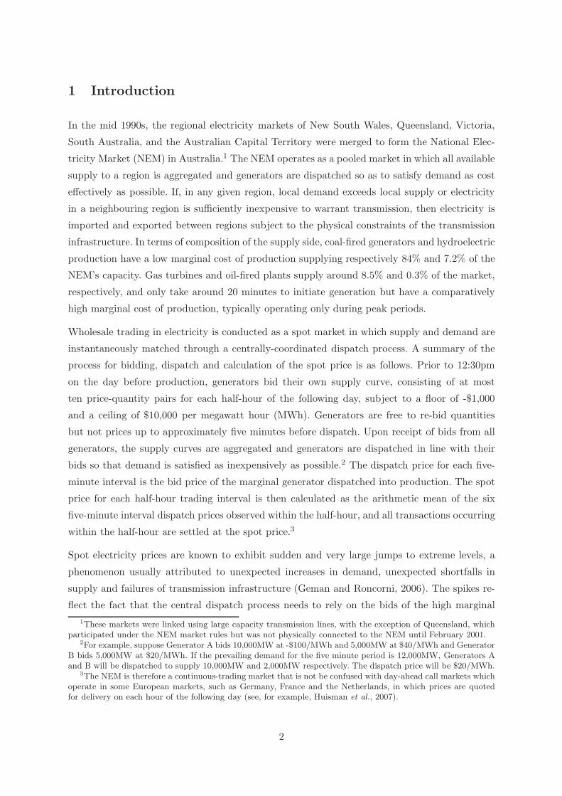
Figure 1: Plot of the median (solid line) and 10th and 90th percentile(dashed lines) spot prices by time of day.
Figure 1 shows the 10th, 50th and 90th percentiles of the half-hourly spot electricity price for
the four regions of the Australian market. It can be seen that spot prices fluctuate between $20
and $40 per MWh under “normal” conditions. The threshold defining an extreme price event in
Australia is generally regarded as $100/MWh which lies above the 90th percentile of spot prices
for each half hour of the day in all regions considered.5 If the spot price exceeds this threshold,
5It is worth noting that other cutoffs were experimented with, namely a variety of percentiles of the uncondi-tional distribution of the price series. The results were not materially affected by the threshold choice. Moreover,the threshold of $100/MWh was deemed by market participants to be the most informative.
9

then a price spike is said to occur and the sequence of these spikes can be regarded as the
realization of a discrete-time point process with the marks of the process representing the severity
of the spikes. Two categories of price spikes are selected,6 namely “mild” if 100 ≤ Pt < 300 and
“severe” if 300 ≤ Pt ≤ 10, 000, where Pt is the spot price at time t. The $300/MWh value is
chosen because it is the strike price of heavily-traded cap products in the Australian market
and the upper limit of $10,000/MWh reflects the price ceiling imposed by the market regulator.
The breakdown of spikes by region is shown in Table 1.
NSW Qld SA Vic
Mild 0.773 0.791 0.881 0.835
Severe 0.227 0.209 0.119 0.165
Total Events 3053 2707 5513 2753
Table 1: Proportion of extreme price events by category. “Mild” refersto prices between $100/MWh and $300/MWh. “Severe” refers to pricesbetween $300/MWh and the market cap of $10,000/MWh.
The econometric model outlined in the preceding section may be applied to this marked point
process to determine the factors driving price spikes. Note that Christensen et al. (2009) find that
the intensity of the true process is significantly related to a historical component and that this
persistence must be accounted for if the resulting econometric model is to be credible.7 In this
application, the persistence of interruptions to the supply side such as plant outages or failure
of the transmission infrastructure can be regarded as stochastic events. The main assumption
made here is that their effects will be primarily captured by the behaviour of the durations u
and ψ that embody the memory of the point process. Of particular interest is the question of
whether or not these durations are still significant in the presence of the other variables believed
to determine extreme events, namely, demand-side variables like load and temperature that are
included as exogenous variables, zt, in the specification of the hazard function in equation (6).
Load directly represents contemporaneous demand because demand is inelastic and must be
balanced with supply at each point in time. Recall that the regulatory framework insulates
consumers from spot price fluctuations, with electricity retailers bearing the spot price risk.
As a consequence, load may be regarded as exogenous. However, the series of half-hourly loads
exhibit a trend in mean and volatility over the sample period and this nonstationarity must
be taken into account. Therefore, the variable Loadt is constructed by de-trending the load at
time t by the mean and standard deviation of the preceding years’ worth of data. This has the
effect of removing any trend in mean and volatility of the load while preserving obvious seasonal
6This choice was informed by correspondence with participants in the Australian electricity market.7Christensen et al. (2009) provide a thorough investigation of the empirical features of electricity price spikes
in the NEM.
10

fluctuations and abnormal load events.
Temperature variables are also expected to influence the occurrence of price spikes through their
influence on demand and on transmission infrastructure. Daily temperature data were provided
by the Australian Bureau of Meteorology, higher-frequency data being unavailable. To correct
for the positive correlation between temperature and price in warm months, and the negative
correlation between temperature and price in cool months, Tmax,t and Tmin,t represent the daily
absolute deviations of the maximum and minimum temperatures from their average over the
preceding 365 days. As a result, the variables Tmax,t and Tmin,t take the same values for all
48 half hour trading intervals on a given day. Of course, the regional markets are state-wide
and substantial variations in temperature are observed within each region. To account for this
as parsimoniously as possible, the temperature observations for the most populous city in each
region were used following Knittel and Roberts (2005).8
The inclusion of the load and temperature variables in the model is potentially problematic
for forecasting because a forecast of the point process at time t based on the information set
at t− 1, requires forecast values for each of the demand-side variables. However, temperature,
and to a lesser extent load, effectively behave as deterministic variables and can be forecast for
the next half-hour or day with a high degree of accuracy (see, for example, Ramanathan et al.,
1997). Consequently, the actual values of these variables at time t will be included as proxies
for their forecast values.
The use of observed variables, particularly load, in the forecasting exercise introduces a potential
distortion. To quantify the effect of using observed load as proxy for forecast load, a primitive
forecasting scheme proposed by Weron (2006) is used as an alternative. This scheme requires
that the forecast load for Saturdays, Sundays and Mondays at each point in time is simply the
load recorded for the same day of the previous week; the forecast for Tuesday through Friday is
given by the load of the previous day. In the NEM all participants have free access to this load
data, so that this forecasting scheme is costless to implement.
4 Estimation
4.1 Estimating the ACH model
The parameters of the ACH model defined by equations (5) and (6) are estimated by maximum
likelihood based on the log-likelihood function in expression (7), with standard errors computed
8Other methods of dealing with growth in level and variability of the load data and the changing direction ofthe relationship of the temperature data with price were investigated. This included removing a linear trend andlinearly scaling the load data, and including the temperature data by season, rather than by absolute deviationfrom the preceding yearly average minimum or maximum temperature. The results were robust to the specificationused.
11
using the typical sandwich procedure employed in quasi-maximum likelihood estimation. The
variable zt in expression (6) consisted of an intercept and the three variables described earlier,
namely Tmax,t, Tmin,t and Loadt.
Table 2 shows the ACH(1, 1) model estimated with all explanatory variables included in zt.
The coefficient of Loadt is positive and significant everywhere, indicating that a higher load
reduces the denominator of expression (6), implying a higher hazard than otherwise. Abnormal
maximum temperatures significantly raise the probability of extreme price events in all regions,
with the exception of SA in which no effect is detected. The marginal effect of abnormal minimum
temperatures only appears to raise the probability of a spike in SA (no effect is detected in the
other regions). When the model was re-estimated with the observed load replaced by the load
forecast (estimates using forecast loads are omitted throughout for brevity) the only material
difference in the estimates was that abnormalities in maximum temperatures have no significant
effect on spike occurrence in SA.
Importantly, however, the parameters embodying the memory or persistence of the spiking pro-
cess, namely, the coefficients on u and ψ remain highly significant notwithstanding the inclusion
of these demand-side variables. Additionally, in line with some specifications of the Poisson jump
intensity popular in the literature, the model was re-estimated using both the current regressors
as well as various dummy variables for diurnal, daily and seasonal factors. This typically added
little to the analysis, with the vast majority of the dummy variables remaining insignificant in
the presence of the load and temperature factors. Importantly the duration factors u and ψ
were still highly significant in the presence of these variables.9 Moreover, the parameter ν varies
greatly across regions, from a near log specification in SA to a super-linear specification in Qld,
and the linear ν = 1 and logarithmic ν = 0 specifications are rejected in all regions based on
likelihood ratio criteria. This suggests that the original linear ACH formulation is inadequate
in this context, and may need to be rethought generally unless one has prior justification for a
linear ARMA duration process.
These results imply that an effective econometric model for extreme events in electricity prices
must account in some way for persistence in the spiking process. This result is significant not
only in the context of the current model, but also has important implications for diffusion models
of spot electricity prices that attempt to incorporate jumps. When a diffusion processes is used
to model the spot price, spikes are usually modeled through the addition of a Poisson jump
component with either a constant intensity parameter (Weron et al., 2004; Cartea and Figueroa,
2005) or a time-varying intensity parameter (Escribano et al., 2002; Knittel and Roberts, 2005)
in which the intensity of the jump process is typically a linear combination of seasonal, weekday
and diurnal effects. A more general conclusion is that any model that drives the intensity of
9The results obtained by estimating these variations are omitted for the sake of brevity.
12
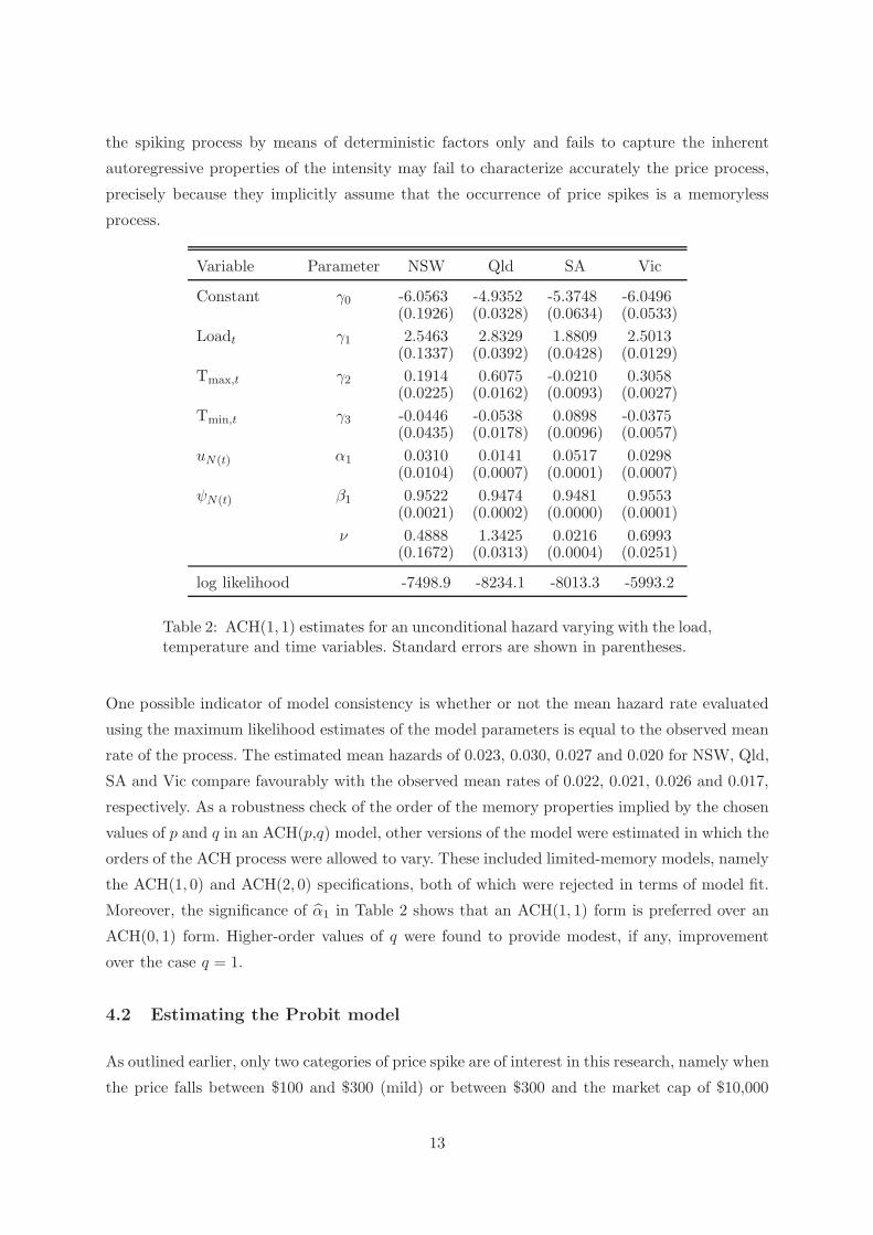
the spiking process by means of deterministic factors only and fails to capture the inherent
autoregressive properties of the intensity may fail to characterize accurately the price process,
precisely because they implicitly assume that the occurrence of price spikes is a memoryless
process.
Variable Parameter NSW Qld SA Vic
Constant γ0 -6.0563 -4.9352 -5.3748 -6.0496(0.1926) (0.0328) (0.0634) (0.0533)
Loadt γ1 2.5463 2.8329 1.8809 2.5013(0.1337) (0.0392) (0.0428) (0.0129)
Tmax,t γ2 0.1914 0.6075 -0.0210 0.3058(0.0225) (0.0162) (0.0093) (0.0027)
Tmin,t γ3 -0.0446 -0.0538 0.0898 -0.0375(0.0435) (0.0178) (0.0096) (0.0057)
uN(t) α1 0.0310 0.0141 0.0517 0.0298(0.0104) (0.0007) (0.0001) (0.0007)
ψN(t) β1 0.9522 0.9474 0.9481 0.9553(0.0021) (0.0002) (0.0000) (0.0001)
ν 0.4888 1.3425 0.0216 0.6993(0.1672) (0.0313) (0.0004) (0.0251)
log likelihood -7498.9 -8234.1 -8013.3 -5993.2
Table 2: ACH(1, 1) estimates for an unconditional hazard varying with the load,temperature and time variables. Standard errors are shown in parentheses.
One possible indicator of model consistency is whether or not the mean hazard rate evaluated
using the maximum likelihood estimates of the model parameters is equal to the observed mean
rate of the process. The estimated mean hazards of 0.023, 0.030, 0.027 and 0.020 for NSW, Qld,
SA and Vic compare favourably with the observed mean rates of 0.022, 0.021, 0.026 and 0.017,
respectively. As a robustness check of the order of the memory properties implied by the chosen
values of p and q in an ACH(p,q) model, other versions of the model were estimated in which the
orders of the ACH process were allowed to vary. These included limited-memory models, namely
the ACH(1, 0) and ACH(2, 0) specifications, both of which were rejected in terms of model fit.
Moreover, the significance of α1 in Table 2 shows that an ACH(1, 1) form is preferred over an
ACH(0, 1) form. Higher-order values of q were found to provide modest, if any, improvement
over the case q = 1.
4.2 Estimating the Probit model
As outlined earlier, only two categories of price spike are of interest in this research, namely when
the price falls between $100 and $300 (mild) or between $300 and the market cap of $10,000
13
(severe). In the Australian market, a price of $100 represents the level at which “peaking”
generators with a high marginal cost of production find it feasible to compete with “baseload”
generators. The $300 price level is the cap for an extensively-used derivative product and $10,000
is the regulated maximum market price. It is anticipated that the variables relating to load and
temperature ought to influence not only the occurrence of extreme price events, but also the
severity of the events. Therefore, the explanatory variables included in the probit analysis are
the same exogenous variables as are used to vary the baseline specification of the hazard rate.
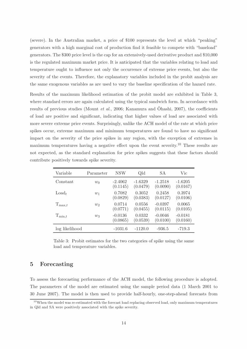
Results of the maximum likelihood estimation of the probit model are exhibited in Table 3,
where standard errors are again calculated using the typical sandwich form. In accordance with
results of previous studies (Mount et al., 2006; Kanamura and Ohashi, 2007), the coefficients
of load are positive and significant, indicating that higher values of load are associated with
more severe extreme price events. Surprisingly, unlike the ACH model of the rate at which price
spikes occur, extreme maximum and minimum temperatures are found to have no significant
impact on the severity of the price spikes in any region, with the exception of extremes in
maximum temperatures having a negative effect upon the event severity.10 These results are
not expected, as the standard explanation for price spikes suggests that these factors should
contribute positively towards spike severity.
Variable Parameter NSW Qld SA Vic
Constant w0 -2.4062 -1.6329 -1.2518 -1.6205(0.1145) (0.0479) (0.0090) (0.0167)
Loadt w1 0.7082 0.3052 0.2458 0.3974(0.0829) (0.0383) (0.0127) (0.0106)
Tmax,t w2 0.0714 0.0556 -0.0397 0.0065(0.0771) (0.0455) (0.0115) (0.0105)
Tmin,t w3 -0.0136 0.0332 -0.0046 -0.0181(0.0865) (0.0539) (0.0100) (0.0160)
log likelihood -1031.6 -1120.0 -936.5 -719.3
Table 3: Probit estimates for the two categories of spike using the sameload and temperature variables.
5 Forecasting
To assess the forecasting performance of the ACH model, the following procedure is adopted.
The parameters of the model are estimated using the sample period data (1 March 2001 to
30 June 2007). The model is then used to provide half-hourly, one-step-ahead forecasts from
10When the model was re-estimated with the forecast load replacing observed load, only maximum temperaturesin Qld and SA were positively associated with the spike severity.
14
a rolling origin of the probability of a price spike for every half-hour interval in the forecast
period 1 July to 30 September 2007. Rolling the forecast origin forward in order to generate
the next half-hourly forecast potentially provides an extra data point for parameter estimation.
For a number of reasons, however, the model parameters are not re-estimated. First, the spot
electricity price is widely regarded as a trend stationary process. Second, even by the end
of the forecast period the additional sample size is negligible compared to the length of the
original estimation period. Third, the sheer size of the estimation sample, 111,648 half-hourly
observations, makes estimation of the model a non-trivial exercise.
The choice of half-hour ahead forecasts is driven by the fact that the NEM operates as a
continuous-trading market up to each half-hour interval. In the event of a price spike being
forecast for the next half-hour interval, effective risk management requires an immediate action
by retailers to mitigate the effects of the potential price spike. Retailers can reduce their reliance
on the pool to meet their demand by activating the standby capacity that they may have
available. Both hydro-electrical and gas-fired peaking plants can be brought from an idle state
to full capacity in half an hour. If this physical response is not available, an alternative strategy
is to use the futures market which trades in real time. An illustration of the use of these half-hour
ahead forecasts to manage price risk using the futures market is provided in Section 5.4.
5.1 A simple benchmark
It has been established that the rate of occurrence of extreme price events depends in part upon
factors relating to load and temperature effects as well as the history of the process. In particular,
the hazard rate is found to depend critically upon factors measuring the recent intensity of
extreme price events, namely the durations and expected durations between neighbouring events.
This ability to model clustering in the spiking process means that the ACH model should
produce forecasts of event probabilities that are superior to those made by models that exclude
a historical component. Therefore in order to assess the forecasting performance of the preferred
model, a benchmark model is required in which the variability of the hazard is attributable to
exogenous variables alone.
The logit model
p t+1 =1
1 + exp(−ξ′zt+1)(8)
provides a straightforward basis for comparative forecast evaluation, where p t+1 is the one-step-
ahead forecast probability of an event occurring at time t+ 1 and zt+1 is a vector of exogenous
variables. This specification of the hazard ignores any information contained in the history of
the process, yet incorporates the variables zt+1 in a functional form similar to that of the ACH
model in expression (6). The log-likelihood is analogous to the log-likelihood function for the
ACH model with the primitive forecast probability p t replacing the conditional hazard ht in
15
expression (7). As argued previously for the ACH model, when forecasting events at time t
conditional on information at time t− 1, actual rather than forecast values for the temperature
variables zt are used, and both observed and primitive forecasts of load are considered separately.
This ensures that both the logit and the ACH model make forecasts using the same information
set, modulo the history of the process itself which is embodied only in the ACH model.
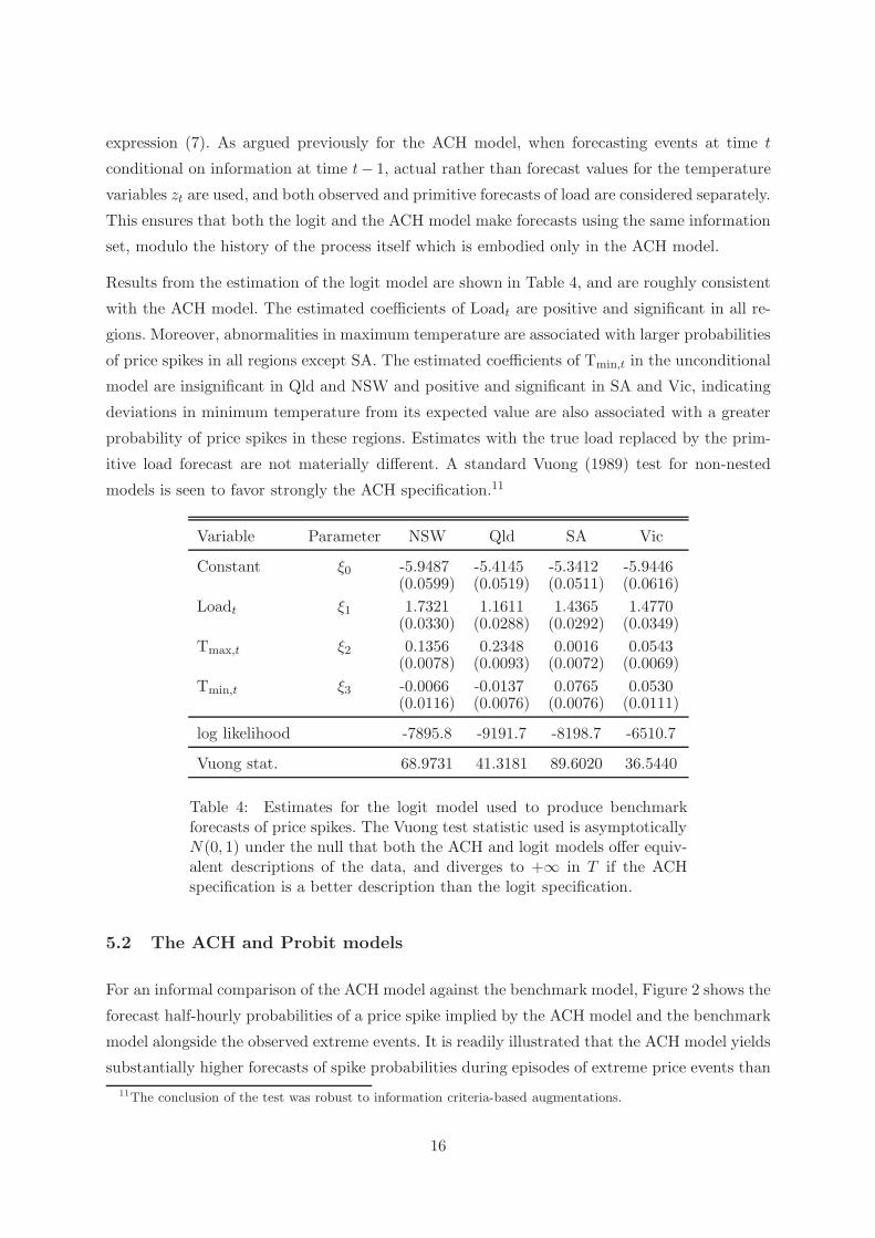
Results from the estimation of the logit model are shown in Table 4, and are roughly consistent
with the ACH model. The estimated coefficients of Loadt are positive and significant in all re-
gions. Moreover, abnormalities in maximum temperature are associated with larger probabilities
of price spikes in all regions except SA. The estimated coefficients of Tmin,t in the unconditional
model are insignificant in Qld and NSW and positive and significant in SA and Vic, indicating
deviations in minimum temperature from its expected value are also associated with a greater
probability of price spikes in these regions. Estimates with the true load replaced by the prim-
itive load forecast are not materially different. A standard Vuong (1989) test for non-nested
models is seen to favor strongly the ACH specification.11
Variable Parameter NSW Qld SA Vic
Constant ξ0 -5.9487 -5.4145 -5.3412 -5.9446(0.0599) (0.0519) (0.0511) (0.0616)
Loadt ξ1 1.7321 1.1611 1.4365 1.4770(0.0330) (0.0288) (0.0292) (0.0349)
Tmax,t ξ2 0.1356 0.2348 0.0016 0.0543(0.0078) (0.0093) (0.0072) (0.0069)
Tmin,t ξ3 -0.0066 -0.0137 0.0765 0.0530(0.0116) (0.0076) (0.0076) (0.0111)
log likelihood -7895.8 -9191.7 -8198.7 -6510.7
Vuong stat. 68.9731 41.3181 89.6020 36.5440
Table 4: Estimates for the logit model used to produce benchmarkforecasts of price spikes. The Vuong test statistic used is asymptoticallyN(0, 1) under the null that both the ACH and logit models offer equiv-alent descriptions of the data, and diverges to +∞ in T if the ACHspecification is a better description than the logit specification.
5.2 The ACH and Probit models
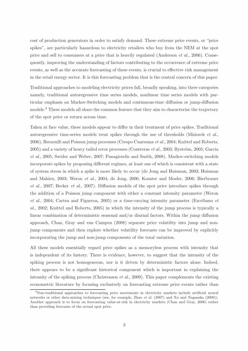
For an informal comparison of the ACH model against the benchmark model, Figure 2 shows the
forecast half-hourly probabilities of a price spike implied by the ACH model and the benchmark
model alongside the observed extreme events. It is readily illustrated that the ACH model yields
substantially higher forecasts of spike probabilities during episodes of extreme price events than
11The conclusion of the test was robust to information criteria-based augmentations.
16

does the simple benchmark model. This is to be expected: the ACH model is able to adapt
its conditional forecasts during episodes of stress, unlike the memoryless benchmark model. A
comparison of the number of actual and predicted events over the forecast period is displayed
in the upper panel of Table 5. Events are said to be forecast correctly if both the forecast
probability calculated at time t for an event at time t+ 1 exceeded a threshold of 0.50 and an
event actually occurred at time t+1. The models were said to trigger false alarms if the forecast
probability exceeded 0.50 but an event did not occur at time t+ 1.
On the basis of this primitive metric, the accuracy of the ACH model in forecasting price spikes
varies from a low of 0% in SA to a high of 48% in NSW. This compares very favourably with
the forecasts from the benchmark model, which failed to identify accurately any price spikes in
Qld, SA and Vic and only 8% in NSW. Similar forecasts of spike probabilities were made using
the forecast load rather than the observed load: the ACH model correctly forecast 0% of events
in SA through to 52% of events in NSW, whereas the benchmark correctly forecast no events
in Qld, SA or Vic and only 5% in NSW.
01-Jul-07 01-Aug-07 01-Sep-07 01-Oct-07
01-Jul-07 01-Aug-07 01-Sep-07 01-Oct-07
01-Jul-07 01-Aug-07 01-Sep-07 01-Oct-07
01-Jul-07 01-Aug-07 01-Sep-07 01-Oct-07
0
0.5
1
0
0.5
1
0
0.5
1
0
0.5
1
Figure 2: ACH(1, 1) forecast probabilities and benchmark logit forecastprobabilities for the first three months following the estimation period.Extreme price events are indicated by a grey vertical bar. The top panelshows the ACH forecast probabilities for NSW, with the second panel show-ing the benchmark forecast probabilities for NSW. The third panel showsthe ACH forecast probabilities for Qld, with the bottom panel showing thebenchmark forecast probabilities for Qld. Similar results are obtained forSA and Vic.
For completeness, the lower panel of Table 5 displays the accuracy of the probit model when
forecasting the intensity of the one-step-ahead events. Because, by construction, the probit
component of the model is independent of the ACH component, these figures refer to all events
that occurred over the forecast period, rather than just the events that were forecast correctly
17
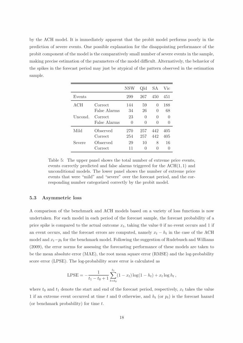
by the ACH model. It is immediately apparent that the probit model performs poorly in the
prediction of severe events. One possible explanation for the disappointing performance of the
probit component of the model is the comparatively small number of severe events in the sample,
making precise estimation of the parameters of the model difficult. Alternatively, the behavior of
the spikes in the forecast period may just be atypical of the pattern observed in the estimation
sample.
NSW Qld SA Vic
Events 299 267 450 451
ACH Correct 144 59 0 188False Alarms 34 26 0 68
Uncond. Correct 23 0 0 0False Alarms 0 0 0 0
Mild Observed 270 257 442 405Correct 254 257 442 405
Severe Observed 29 10 8 16Correct 11 0 0 0
Table 5: The upper panel shows the total number of extreme price events,events correctly predicted and false alarms triggered for the ACH(1, 1) andunconditional models. The lower panel shows the number of extreme priceevents that were “mild” and “severe” over the forecast period, and the cor-responding number categorized correctly by the probit model.
5.3 Asymmetric loss
A comparison of the benchmark and ACH models based on a variety of loss functions is now
undertaken. For each model in each period of the forecast sample, the forecast probability of a
price spike is compared to the actual outcome xt, taking the value 0 if no event occurs and 1 if
an event occurs, and the forecast errors are computed, namely xt − ht in the case of the ACH
model and xt−pt for the benchmark model. Following the suggestion of Rudebusch and Williams
(2009), the error norms for assessing the forecasting performance of these models are taken to
be the mean absolute error (MAE), the root mean square error (RMSE) and the log-probability
score error (LPSE). The log-probability score error is calculated as
LPSE = −1
t1 − t0 + 1
t1∑
t=t0
(1 − xt) log(1 − ht) + xt log ht ,
where t0 and t1 denote the start and end of the forecast period, respectively, xt takes the value
1 if an extreme event occurred at time t and 0 otherwise, and ht (or pt) is the forecast hazard
(or benchmark probability) for time t.
18
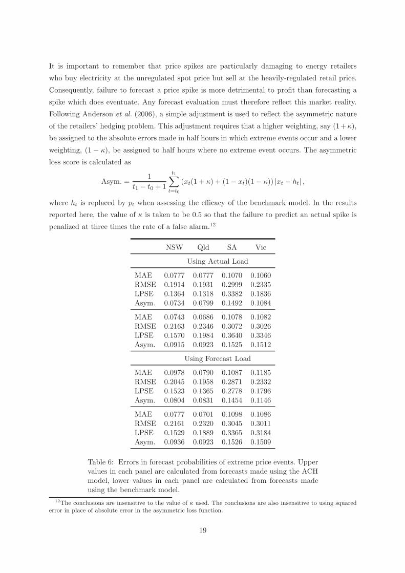
It is important to remember that price spikes are particularly damaging to energy retailers
who buy electricity at the unregulated spot price but sell at the heavily-regulated retail price.
Consequently, failure to forecast a price spike is more detrimental to profit than forecasting a
spike which does eventuate. Any forecast evaluation must therefore reflect this market reality.
Following Anderson et al. (2006), a simple adjustment is used to reflect the asymmetric nature
of the retailers’ hedging problem. This adjustment requires that a higher weighting, say (1+κ),
be assigned to the absolute errors made in half hours in which extreme events occur and a lower
weighting, (1 − κ), be assigned to half hours where no extreme event occurs. The asymmetric
loss score is calculated as
Asym. =1
t1 − t0 + 1
t1∑
t=t0
(xt(1 + κ) + (1 − xt)(1 − κ)) |xt − ht| ,
where ht is replaced by pt when assessing the efficacy of the benchmark model. In the results
reported here, the value of κ is taken to be 0.5 so that the failure to predict an actual spike is
penalized at three times the rate of a false alarm.12
NSW Qld SA Vic
Using Actual Load
MAE 0.0777 0.0777 0.1070 0.1060RMSE 0.1914 0.1931 0.2999 0.2335LPSE 0.1364 0.1318 0.3382 0.1836Asym. 0.0734 0.0799 0.1492 0.1084
MAE 0.0743 0.0686 0.1078 0.1082RMSE 0.2163 0.2346 0.3072 0.3026LPSE 0.1570 0.1984 0.3640 0.3346Asym. 0.0915 0.0923 0.1525 0.1512
Using Forecast Load
MAE 0.0978 0.0790 0.1087 0.1185RMSE 0.2045 0.1958 0.2871 0.2332LPSE 0.1523 0.1365 0.2778 0.1796Asym. 0.0804 0.0831 0.1454 0.1146
MAE 0.0777 0.0701 0.1098 0.1086RMSE 0.2161 0.2320 0.3045 0.3011LPSE 0.1529 0.1889 0.3365 0.3184Asym. 0.0936 0.0923 0.1526 0.1509
Table 6: Errors in forecast probabilities of extreme price events. Uppervalues in each panel are calculated from forecasts made using the ACHmodel, lower values in each panel are calculated from forecasts madeusing the benchmark model.
12The conclusions are insensitive to the value of κ used. The conclusions are also insensitive to using squarederror in place of absolute error in the asymmetric loss function.
19
The results of this comparative exercise are displayed in Table 6. The ACH model forecasts with
lower RMSE and LPSE than the benchmark model in all regions, and also with lower MAE in SA
and VIC, when the observed load is used in forecasting spike probabilities. The most dramatic
difference in forecast error between the ACH and benchmark models is recorded by the LPS
measure, which Rudebusch and Williams (2009) suggest is the most appropriate for evaluating
forecast probabilities. The ACH model also achieved lower errors using the asymmetric metric.
Importantly, the superior forecast performance (at least in terms of these error metrics) of the
ACH model over the benchmark model persists when the observed load is replaced with the
primitive load forecast. This suggests that the results reported here are not merely driven by
the use of actual load, a variable which may not be made public quickly enough to generate
real-time, half-hour ahead forecasts.
5.4 A simple trading scheme
As noted earlier, the forecast horizon of three months used for forecast evaluation is chosen to
correspond to the duration of a typical futures contract in the electricity market. Consequently,
to complement the results of the forecast error comparison presented previously, the forecasts
generated by the model can be used to explore the profitability of an informal trading scheme
based on electricity futures contracts. The results of this exercise should be interpreted more as
an illustration of the forecast performance of the ACH and benchmark models than evidence of
a profitable futures trading strategy as the experiment suffers from a number of shortcomings.
In particular, no intra-day futures prices are available so synthetic contracts are priced artifi-
cially. In addition, transaction costs are ignored (though conversation with market participants
suggested that these are minor).
A quarterly futures contract is available in the Australian electricity market which fixes the price
of electricity to the retailer for the life of the contract. Specifically, at time t during the life of
the contract, the hedged price in terms of the futures contract is calculated as the time-weighted
average of the following components:
(i) the mean of the actual spot electricity price for each half hour from the start of the contract
to the current time t, and
(ii) the mean of the consensus of analysts’ forecasts of price for each half hour for the remainder
of the contract.
As no futures prices or consensus forecasts are publicly available, synthetic futures contracts are
priced by taking the consensus forecast of price to be the average price for the same half hour
on the same weekday in the same month for the previous five years for the relevant region.
20
The simple trading strategy proposed here is as follows. If at time t − 1 the one-step-ahead
probability of a price spike at time t exceeds a threshold probability of 0.5, the futures contract
is entered into. The contract is closed out at time t + k provided the forecast probability of a
spike exceeds the threshold in each interval up to time t + k but falls below threshold at time
t + k + 1. The return to this strategy is therefore the difference between the actual pool price
and the hedged price specified in terms of the futures contract.
Implementing this trading scheme in the NSW market over the out-of-sample period using a
threshold probability of 0.5 resulted in a return over the period of 21.47%. To compare the
significance of this return to the distribution of returns generated using the benchmark model,
10, 000 samples of the length of the forecast period were drawn from the U [0, 1] distribution.
For each sample, a spike is forecast in a given half-hour if the benchmark probability of a
spike exceeds the random draw for that interval. This ensures that the distribution of simulated
spikes matches that implied by the benchmark model. The trading strategy was implemented
for each sample using these forecasts. The 99th percentile return to this strategy was 14.53%
over the same period indicating that using the futures market as a hedge based on the forecasts
of the ACH model has the potential to provide significant returns. Implementing the strat-
egy in Qld, SA and Vic gave returns of 8.02%, 0% (no trades occurred) and 24.22%, whereas
the 99th percentiles computed in terms of the unconditional forecasts were 6.21%, 2.80% and
5.87%, respectively. Similar results were obtained using the primitive load forecast in place of
actual load. With the exception of SA, the outcome of this simple simulated trading scheme
provides additional evidence of the usefulness of the ACH model in forecasting extreme events
in electricity markets.
6 Conclusion
Accurate forecasting of extreme price events is of great importance for risk management in the
electricity sector. The overwhelming majority of electricity-pricing models are adaptations of
popular models for price or returns from the financial econometrics literature that have been
augmented to capture the idiosyncratic time-series properties of electricity prices, with varying
degrees of success. By contrast, this paper focuses solely on the forecasting of extreme price
events, the occurrence of which is treated as a realization of a discrete-time point process. An
ACH framework is used to analyze the drivers of the process and to forecast the probability of
extreme price events occurring in real time. Abnormal loads were found to have a significant
impact upon the probability of a price spike and on the severity of the spike, and temperature
extremes were found to influence the rate at which spikes occurred, but not their severity.
Importantly, stochastic factors capturing the history of the process were found to be significant
in explaining the occurrence of extreme price events. Specifically, durations between price spikes
21

were found to depend nonlinearly on previous expected and observed durations.
The ACH model is shown to provide rolling half-hour ahead forecasts of price spikes that are
superior to forecasts made on the same set of exogenous information using a memoryless model.
In addition, the returns generated from a simple synthetic futures trading scheme based on the
one-step-ahead forecast probabilities of the ACH model provide further evidence of the strength
of the model in forecasting electricity price spikes.
22
References
Anderson, E. J., Hu, X. and Winchester, D. (2006). Forward contracts in electricity markets:The Australian experience. Energy Policy, 35, 3089–3103.
Barlow, M. T. (2002). A diffusion model for electricity prices. Mathematical Finance, 12, 287–298.
Bauwens, L. and Giot, P. (2000). The logarithmic ACD Model: An application to the bid-askquote process of three NYSE stocks. Annales d’Economie et de Statistique, 60, 117–149.
Bauwens, L. and Veredas, D. (2004). The stochastic conditional duration model: a latent vari-able model for the analysis of financial durations. Journal of Econometrics, 119, 381–412.
Becker, R., Hurn, A. S. and Pavlov, V. (2007). Modelling spikes in electricity prices. Economic
Record, 83, 371–382.
Bierbrauer, M., Menn, C., Rachev S. T. and Truck, S. (2007). Spot and derivative pricing inthe EEX power market. Journal of Banking and Finance, 31, 3462–3485.
Bystrom, H. N. E. (2005). Extreme value theory and extremely large electricity price changes.International Review of Economics and Finance, 14, 41–55.
Cartea, A. and Figueroa, M. G. (2005). Pricing in electricity markets: A mean reverting jumpdiffusion model with seasonality. Applied Mathematical Finance, 12, 313–335.
Chan, K.F. and Gray, P. (2006). Using extreme value theory to measure value-at-risk for dailyelectricity spot prices. International Journal of Forecasting, 22, 283–300.
Chan, K.F., Gray, P. and van Campen, B. (2008). A new approach to characterizing andforecasting electricity price volatility. International Journal of Forecasting, 24, 728–743.
Christensen, T.M., Hurn, A.S. and Lindsay, K.A. (2009) It never rains but it pours: Modellingthe persistence of spikes in electricity prices. The Energy Journal, 30, 25–48.
Contreras, J., Espınola, R., Nogales, F. J. and Conejo, A. J. (2003). ARIMA models to predictnext-day electricity prices. IEEE Transactions on Power Systems, 18, 1014–1020.
Crespo Cuaresma, J., Hlouskova, J., Kossmeier, C. and Obersteiner, M. (2004). Forecastingelectricity spot-prices using linear univariate time-series models. Applied Energy, 77, 87–106.
de Jong, C. (2006). The nature of power spikes: A regime-switching approach. Studies in
Nonlinear Dynamics and Econometrics, 10.
de Jong, C. and Huisman, R. (2003). Option pricing for power prices with spikes. Energy Power
Risk Management, 7, 12–16.
Engle, R. F. and Russell, J. R. (1997). Forecasting the frequency of changes in quoted for-eign exchange prices with the autoregressive conditional duration model. Journal of Empirical
Finance, 4, 187–212.
Engle, R. F. and Russell, J. R. (1998). Autoregressive conditional duration: A new model forirregularly spaced transaction data. Econometrica, 66, 1127–1162.
23

Engle, R. F. (2000). The econometrics of ultra-high-frequency data. Econometrica, 68, 1–22.
Engle, R. F. and Dufour, A. (2000). The ACD Model: Predictability of the Time BetweenConsecutive Trades. Discussion Paper in Finance 2000-05, University of Reading.
Engle, R. F. and Russell, J. R. (2005). A discrete-state continuous-time model of financialtransactions prices and times: The autoregressive conditional multinomial–Autoregressive Con-ditional Duration model. Journal of Business and Economics Statistics, 23, 166–180.
Escribano, A, Pena, J. I. and Villaplana, P. (2002). Modelling electricity prices: Internationalevidence. Working Paper 02-27, Universidad Carlos III de Madrid.
Feng, G., Jiang, G. J. and Song, P. X.-K. (2004). Stochastic conditional duration models with“leverage effect” for financial transaction data. Journal of Financial Econometrics, 2, 390–421.
Fernandes, M. and Grammig, J. (2006). A family of autoregressive conditional duration models.Journal of Econometrics, 130, 1–23.
Garcia, R. C., Contreras, J., van Akkeren, M. and Garcia, J. B. C., (2005). A GARCH fore-casting model to predict day-ahead electricity prices. IEEE Transactions on Power Systems,20, 867–874.
Geman, H. and Roncorni, A. (2006). Understanding the fine structure of electricity prices.Journal of Business, 79, 1225–1261.
Hamilton, J. D. and Jorda, O. (2002). A model of the Federal Funds Rate target. Journal of
Political Economy, 110, 1135–1167.
Huisman, R. and Mahieu, R. (2003). Regime jumps in electricity prices. Energy Economics,25, 425–434.
Huisman, R., Huurman, C. amd Mahieu R. (2007). Hourly electricity prices in day-aheadmarkets. Energy Economics, 29, 240–248.
Kanamura, T. and Ohashi, K. (2007). On transition probabilities of regime switching in elec-tricity prices. Energy Economics, 30, 1158–1172.
Knittel, C. R. and Roberts, M. R. (2005). An empirical examination of restructured electricityprices. Energy Economics, 27, 791–817.
Kosater, P. and Mosler, K. (2006). Can Markov regime-switching models improve power-priceforecasts? Evidence from German daily power prices. Applied Energy, 83, 943—958.
Misiorek, A., Truck, S. and Weron, R. (2006). Point and interval forecasting of spot electricityprices: Linear vs. non-linear time series models. Studies in Nonlinear Dynamics and Econo-
metrics, 10.
Mount, T. D., Ning, Y. and Cai, X. (2006). Predicting price spikes in electricity markets usinga regime-switching model with time-varying parameters. Energy Economics, 28, 62–80.
Panagiotelis, A. and Smith, M. (2008). Bayesian density forecasting of intraday electricity pricesusing multivariate skew t distributions. International Journal of Forecasting, 24, 710–727.
Ramanathan, R., Engle, R. F., Granger, C. W. J., Vahid-Araghi, F. and Brace, C. (1997).Short-run forecasts of electricity loads and peaks. International Journal of Forecasting, 13,161–174.
24

Rudebusch, G. D. and Williams, J. C. (2009). Forecasting recessions: the puzzle of the enduringpower of the yield curve. Journal of Business and Economic Statistics, 27, 492–503.
Swider, D. J. and Weber, C. (2007). Extended ARMA models for estimating price developmentson day-ahead electricity markets. Electric Power Systems Research, 77, 583–593.
Vuong, Q. H. (1989). Likelihood Ratio Tests for Model Selection and Non-Nested Hypotheses.Econometrica, 57(2), 307–333.
Weron, R., Bierbrauer, M. and Truck, S. (2004). Modelling electricity prices: jump diffusionand regime switching. Physica A, 336, 39–48.
Weron, R. Modelling and Forecasting Electricity Loads and Prices: A Statistical Approach.
John Wiley and Sons, Ltd.: Chichester.
Xu, Y, and Nagasaka, K. (2009) Demand and price forecasting by artificial neural networks(ANNs) in a deregulated power market. International Journal of Electrical and Power Engi-
neering, 3, 268–275.
Zhang, M. Y., Russell, J. R. and Tsay, R. S. (2001). A nonlinear autoregressive conditionalduration model with applications to financial transaction data. Journal of Econometrics, 104,179–207.
Zhao, J.H., Dong, Z.Y. and Li, X. (2007), Electricity market price spike forecasting and decisionmaking. IET Generation Transmission and Distribution, 1, 647–654.
25

List of NCER Working Papers
No. 69 (Download full text) Don Harding and Adrian Pagan
Can We Predict Recessions?
No. 68 (Download full text) Amir Rubin and Daniel Smith
Comparing Different Explanations of the Volatility Trend
No. 67 (Download full text) Wagner Piazza Gaglianone, Luiz Renato Lima, Oliver Linton and Daniel Smith
Evaluating Value-at-Risk Models via Quantile Regression
No. 66 (Download full text) Ralf Becker, Adam Clements and Robert O’Neill
A Kernel Technique for Forecasting the Variance-Covariance Matrix
No. 65 (Download full text) Stan Hurn, Andrew McClelland and Kenneth Lindsay
A quasi-maximum likelihood method for estimating the parameters of multivariate diffusions
No. 64 (Download full text) Ralf Becker and Adam Clements
Volatility and the role of order book structure?
No. 63 (Download full text) Adrian Pagan
Can Turkish Recessions be Predicted?
No. 62 (Download full text) Lionel Page and Katie Page
Evidence of referees’ national favouritism in rugby
No. 61 (Download full text) Nicholas King, P Dorian Owen and Rick Audas
Playoff Uncertainty, Match Uncertainty and Attendance at Australian National Rugby League Matches
No. 60 (Download full text) Ralf Becker, Adam Clements and Robert O'Neill
A Cholesky-MIDAS model for predicting stock portfolio volatility
No. 59 (Download full text) P Dorian Owen Measuring Parity in Sports Leagues with Draws: Further Comments

No. 58 (Download full text) Don Harding Applying shape and phase restrictions in generalized dynamic categorical models of the business cycle
No. 57 (Download full text) Renee Fry and Adrian Pagan Sign Restrictions in Structural Vector Autoregressions: A Critical Review
No. 56 (Download full text) Mardi Dungey and Lyudmyla Hvozdyk Cojumping: Evidence from the US Treasury Bond and Futures Markets
No. 55 (Download full text) Martin G. Kocher, Marc V. Lenz and Matthias Sutter Psychological pressure in competitive environments: Evidence from a randomized natural experiment: Comment
No. 54 (Download full text) Adam Clements and Annastiina Silvennoinen Estimation of a volatility model and portfolio allocation
No. 53 (Download full text) Luis Catão and Adrian Pagan The Credit Channel and Monetary Transmission in Brazil and Chile: A Structured VAR Approach No. 52 (Download full text) Vlad Pavlov and Stan Hurn Testing the Profitability of Technical Analysis as a Portfolio Selection Strategy
No. 51 (Download full text) Sue Bridgewater, Lawrence M. Kahn and Amanda H. Goodall Substitution Between Managers and Subordinates: Evidence from British Football
No. 50 (Download full text) Martin Fukac and Adrian Pagan Structural Macro-Econometric Modelling in a Policy Environment
No. 49 (Download full text) Tim M Christensen, Stan Hurn and Adrian Pagan Detecting Common Dynamics in Transitory Components
No. 48 (Download full text) Egon Franck, Erwin Verbeek and Stephan Nüesch
Inter-market Arbitrage in Sports Betting
No. 47 (Download full text) Raul Caruso Relational Good at Work! Crime and Sport Participation in Italy. Evidence from Panel Data Regional Analysis over the Period 1997-2003.

No. 46 (Download full text) (Accepted) Peter Dawson and Stephen Dobson The Influence of Social Pressure and Nationality on Individual Decisions: Evidence from the Behaviour of Referees
No. 45 (Download full text) Ralf Becker, Adam Clements and Christopher Coleman-Fenn
Forecast performance of implied volatility and the impact of the volatility risk premium
No. 44 (Download full text) Adam Clements and Annastiina Silvennoinen
On the economic benefit of utility based estimation of a volatility model
No. 43 (Download full text) Adam Clements and Ralf Becker
A nonparametric approach to forecasting realized volatility
No. 42 (Download full text) Uwe Dulleck, Rudolf Kerschbamer and Matthias Sutter
The Economics of Credence Goods: On the Role of Liability, Verifiability, Reputation and Competition
No. 41 (Download full text)Adam Clements, Mark Doolan, Stan Hurn and Ralf Becker
On the efficacy of techniques for evaluating multivariate volatility forecasts
No. 40 (Download full text) Lawrence M. Kahn
The Economics of Discrimination: Evidence from Basketball
No. 39 (Download full text) Don Harding and Adrian Pagan
An Econometric Analysis of Some Models for Constructed Binary Time Series
No. 38 (Download full text) Richard Dennis
Timeless Perspective Policymaking: When is Discretion Superior?
No. 37 (Download full text) Paul Frijters, Amy Y.C. Liu and Xin Meng Are optimistic expectations keeping the Chinese happy? No. 36 (Download full text) Benno Torgler, Markus Schaffner, Bruno S. Frey, Sascha L. Schmidt and Uwe Dulleck Inequality Aversion and Performance in and on the Field No. 35 (Download full text) T M Christensen, A. S. Hurn and K A Lindsay Discrete time-series models when counts are unobservable

No. 34 (Download full text) Adam Clements, A S Hurn and K A Lindsay Developing analytical distributions for temperature indices for the purposes of pricing temperature-based weather derivatives No. 33 (Download full text) Adam Clements, A S Hurn and K A Lindsay Estimating the Payoffs of Temperature-based Weather Derivatives No. 32 (Download full text) T M Christensen, A S Hurn and K A Lindsay The Devil is in the Detail: Hints for Practical Optimisation No. 31 (Download full text) Uwe Dulleck, Franz Hackl, Bernhard Weiss and Rudolf Winter-Ebmer Buying Online: Sequential Decision Making by Shopbot Visitors No. 30 (Download full text) Richard Dennis Model Uncertainty and Monetary Policy No. 29 (Download full text) Richard Dennis The Frequency of Price Adjustment and New Keynesian Business Cycle Dynamics No. 28 (Download full text) Paul Frijters and Aydogan Ulker Robustness in Health Research: Do differences in health measures, techniques, and time frame matter? No. 27 (Download full text) Paul Frijters, David W. Johnston, Manisha Shah and Michael A. Shields Early Child Development and Maternal Labor Force Participation: Using Handedness as an Instrument No. 26 (Download full text) Paul Frijters and Tony Beatton The mystery of the U-shaped relationship between happiness and age. No. 25 (Download full text) T M Christensen, A S Hurn and K A Lindsay It never rains but it pours: Modelling the persistence of spikes in electricity prices No. 24 (Download full text) Ralf Becker, Adam Clements and Andrew McClelland The Jump component of S&P 500 volatility and the VIX index No. 23 (Download full text) A. S. Hurn and V.Pavlov Momentum in Australian Stock Returns: An Update

No. 22 (Download full text) Mardi Dungey, George Milunovich and Susan Thorp Unobservable Shocks as Carriers of Contagion: A Dynamic Analysis Using Identified Structural GARCH No. 21 (Download full text) (forthcoming) Mardi Dungey and Adrian Pagan Extending an SVAR Model of the Australian Economy No. 20 (Download full text) Benno Torgler, Nemanja Antic and Uwe Dulleck Mirror, Mirror on the Wall, who is the Happiest of Them All? No. 19 (Download full text) Justina AV Fischer and Benno Torgler Social Capital And Relative Income Concerns: Evidence From 26 Countries No. 18 (Download full text) Ralf Becker and Adam Clements Forecasting stock market volatility conditional on macroeconomic conditions. No. 17 (Download full text) Ralf Becker and Adam Clements Are combination forecasts of S&P 500 volatility statistically superior? No. 16 (Download full text) Uwe Dulleck and Neil Foster Imported Equipment, Human Capital and Economic Growth in Developing Countries No. 15 (Download full text) Ralf Becker, Adam Clements and James Curchin Does implied volatility reflect a wider information set than econometric forecasts? No. 14 (Download full text) Renee Fry and Adrian Pagan Some Issues in Using Sign Restrictions for Identifying Structural VARs No. 13 (Download full text) Adrian Pagan Weak Instruments: A Guide to the Literature No. 12 (Download full text) Ronald G. Cummings, Jorge Martinez-Vazquez, Michael McKee and Benno Torgler Effects of Tax Morale on Tax Compliance: Experimental and Survey Evidence No. 11 (Download full text) Benno Torgler, Sascha L. Schmidt and Bruno S. Frey The Power of Positional Concerns: A Panel Analysis

No. 10 (Download full text) Ralf Becker, Stan Hurn and Vlad Pavlov Modelling Spikes in Electricity Prices No. 9 (Download full text) A. Hurn, J. Jeisman and K. Lindsay Teaching an Old Dog New Tricks: Improved Estimation of the Parameters of Stochastic Differential Equations by Numerical Solution of the Fokker-Planck Equation No. 8 (Download full text) Stan Hurn and Ralf Becker Testing for nonlinearity in mean in the presence of heteroskedasticity. No. 7 (Download full text) (published) Adrian Pagan and Hashem Pesaran On Econometric Analysis of Structural Systems with Permanent and Transitory Shocks and Exogenous Variables. No. 6 (Download full text) (published) Martin Fukac and Adrian Pagan Limited Information Estimation and Evaluation of DSGE Models. No. 5 (Download full text) Andrew E. Clark, Paul Frijters and Michael A. Shields
Income and Happiness: Evidence, Explanations and Economic Implications.
No. 4 (Download full text) Louis J. Maccini and Adrian Pagan Inventories, Fluctuations and Business Cycles. No. 3 (Download full text) Adam Clements, Stan Hurn and Scott White Estimating Stochastic Volatility Models Using a Discrete Non-linear Filter. No. 2 (Download full text) Stan Hurn, J.Jeisman and K.A. Lindsay Seeing the Wood for the Trees: A Critical Evaluation of Methods to Estimate the Parameters of Stochastic Differential Equations. No. 1 (Download full text) Adrian Pagan and Don Harding The Econometric Analysis of Constructed Binary Time Series.
Recommended