Gaussian Processes
Daniel McDuff
MIT Media Lab
December 2, 2010
Daniel McDuff (MIT Media Lab) Gaussian Processes December 2, 2010 1 / 44

Quote of the Day
”Only in Britain could it be thought a defect to be too clever
by half. The probability is that too many people are too stupid
by three-quarters.”
Former Prime Minister John Major assessing the priors on intelligencein the UK.
Daniel McDuff (MIT Media Lab) Gaussian Processes December 2, 2010 2 / 44

Outline
1 Introduction
2 Theory
3 Regression
4 Classification
5 Applications
6 Summary
Daniel McDuff (MIT Media Lab) Gaussian Processes December 2, 2010 3 / 44
Introduction
Introduction
Books and Resources
Gaussian Processes for Machine Learning - C. Rasmussen and C.Williams. MATLAB code to accompany.
Information Theory, Inference, and Learning Algorithms - D. Mackay.
Video tutorials, slides, software: www.gaussianprocess.org
Daniel McDuff (MIT Media Lab) Gaussian Processes December 2, 2010 4 / 44
Introduction
Notation
D = Training dataset, { (xi , y) | i= 1,...n }x = Training feature vectorX = Training featuresy = Training labelsx* = Test feature vectory* = Test labelsGP(m(x), k(x, x’)) = Gaussian process with mean function, m(x), andcovariance function, k(x, x’).
Daniel McDuff (MIT Media Lab) Gaussian Processes December 2, 2010 5 / 44
Introduction
Parametric Models vs. Non-parametric Models
Non-parametric models differ from parametric models. The modelstructure is not specified a priori but is determined from the data.
Parametric models:
Support Vector Machines
Neural Networks
Non-parametric models:
KNN
Gaussian processes
Daniel McDuff (MIT Media Lab) Gaussian Processes December 2, 2010 6 / 44
Introduction
Supervised Learning
Our Problem: To map from finite training examples to a function thatpredicts for all possible inputs.
Restrict the solution functions that we consider. Example: Linearregression.
-ve: If wrong form of function is chosen then predictions will be poor.
Apply prior probabilities to functions that we consider more likely.
-ve: Infinite possibilities of functions to consider.
Daniel McDuff (MIT Media Lab) Gaussian Processes December 2, 2010 7 / 44
Theory
Theory
Definition: A Gaussian process is a collection of random variables, anyfinite number of which have a joint Gaussian distribution.
A Gaussian process is a generalization of the Gaussian probabilitydistribution.
It is a distribution over functions rather a distribution over vectors.
It is a non-parametric method of modeling data.
A Gaussian Process is of infinite dimensions. However, we only workwith a finite subset.
Fortunately, this yields the same inference as if we were to consider allthe infinite possibilities.
Daniel McDuff (MIT Media Lab) Gaussian Processes December 2, 2010 8 / 44
Theory
Theory
Gaussian distributions
N (µ,Σ)
Distribution over vectors.Fully specified by a mean andcovariance.The position of the randomvariable in the vector plays therole of the index.
Gaussian processes
GP(m(x), k(x, x’))
Distribution over functions.Fully specified by a meanfunction and covariancefunction.The argument of the randomfunction plays the role of theindex.
Daniel McDuff (MIT Media Lab) Gaussian Processes December 2, 2010 9 / 44
Theory
Theory
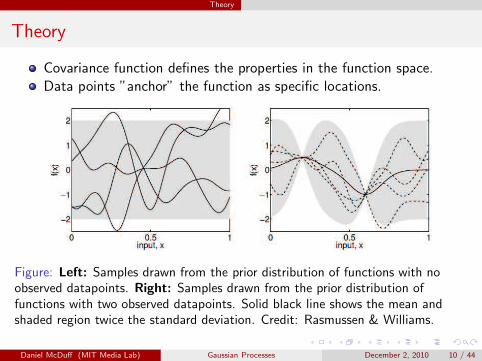
Covariance function defines the properties in the function space.
Data points ”anchor” the function as specific locations.
Figure: Left: Samples drawn from the prior distribution of functions with noobserved datapoints. Right: Samples drawn from the prior distribution offunctions with two observed datapoints. Solid black line shows the mean andshaded region twice the standard deviation. Credit: Rasmussen & Williams.
Daniel McDuff (MIT Media Lab) Gaussian Processes December 2, 2010 10 / 44
Theory
Theory
What do we need to define?
Mean function, m(x) - Usually defined to be zero. Justified bymanipulating the data.
Covariance function,k(x, x’) - This defines the prior properties of thefunctions considered for inference.
StationaritySmoothnessLength-scales
Gaussian processes provide a well defined approach for learning model andhyperparameters from the data.
Daniel McDuff (MIT Media Lab) Gaussian Processes December 2, 2010 11 / 44
Regression
Regression
Prediction of continuous quantity, y, from input, x*.
We will assume the prediction to have two parts:
A systematic variation: Accurately predicted by an underlying processf (x).
A random variation: Unpredictability of the system.
The result:
yi = f (xi ) + ǫi (1)
Daniel McDuff (MIT Media Lab) Gaussian Processes December 2, 2010 12 / 44
Regression
Bayesian Linear Regression
A simple example of Gaussian Processes:
y = xTw+ ǫ (2)
Estimate a distribution over weights.
Marginalise over weights to derive prediction.
Predictive distribution:
f∗|x∗,X , y = N (xT∗A−1X y, xT
∗A−1x∗) (3)
Daniel McDuff (MIT Media Lab) Gaussian Processes December 2, 2010 13 / 44
Regression
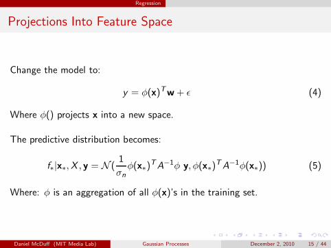
Projections Into Feature Space
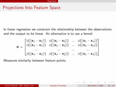
In linear regression we constrain the relationship between the observationsand the output to be linear. An alternative is to use a kernel:
Φ =
φ(||x1 − x1||) φ(||x1 − x2||) ... φ(||x1 − xn||)φ(||x2 − x1||) φ(||x2 − x2||) ... φ(||x2 − xn||)
... ... ... ...
φ(||xn − x1||) φ(||xn − x2||) ... φ(||x1 − xn||)
Measures similarity between feature points.
Daniel McDuff (MIT Media Lab) Gaussian Processes December 2, 2010 14 / 44
Regression
Projections Into Feature Space
Change the model to:
y = φ(x)Tw+ ǫ (4)
Where φ() projects x into a new space.
The predictive distribution becomes:
f∗|x∗,X , y = N (1
σnφ(x∗)
TA−1φ y, φ(x∗)TA−1φ(x∗)) (5)
Where: φ is an aggregation of all φ(x)’s in the training set.
Daniel McDuff (MIT Media Lab) Gaussian Processes December 2, 2010 15 / 44
Regression
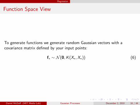
Function Space View
To generate functions we generate random Gaussian vectors with acovariance matrix defined by your input points:
f∗ ∼ N (0,K (X∗,X∗)) (6)
Daniel McDuff (MIT Media Lab) Gaussian Processes December 2, 2010 16 / 44
Regression
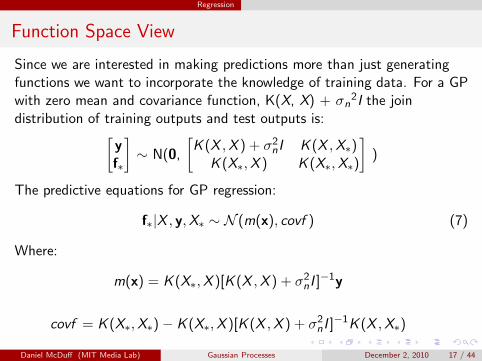
Function Space View
Since we are interested in making predictions more than just generatingfunctions we want to incorporate the knowledge of training data. For a GPwith zero mean and covariance function, K(X, X) + σn
2I the joindistribution of training outputs and test outputs is:
[
y
f∗
]
∼ N(0,
[
K (X ,X ) + σ2nI K (X ,X∗)
K (X∗,X ) K (X∗,X∗)
]
)
The predictive equations for GP regression:
f∗|X , y,X∗ ∼ N (m(x), covf ) (7)
Where:
m(x) = K (X∗,X )[K (X ,X ) + σ2nI ]
−1y
covf = K (X∗,X∗)− K (X∗,X )[K (X ,X ) + σ2nI ]
−1K (X ,X∗)
Daniel McDuff (MIT Media Lab) Gaussian Processes December 2, 2010 17 / 44
Regression
MATLAB Example
MATLAB Example. Code adapted from GPML demo - gaussianprocess.org
Daniel McDuff (MIT Media Lab) Gaussian Processes December 2, 2010 18 / 44
Regression
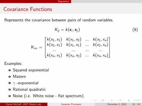
Covariance Functions
Represents the covariance between pairs of random variables.
Kij = k(xi , xj) (8)
Kxx =
k(x1, x1) k(x1, x2) ... k(x1, xn)k(x2, x1) k(x1, x1) ... k(x2, xn)
... ... ... ...
k(xn, x1) k(xn, x2) ... k(xn, xn)
Examples:
Squared exponential
Matern
γ -exponential
Rational quadratic
Noise (i.e. White noise - flat spectrum).
Daniel McDuff (MIT Media Lab) Gaussian Processes December 2, 2010 19 / 44
Regression
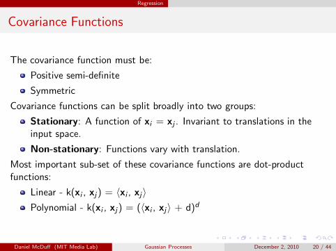
Covariance Functions
The covariance function must be:
Positive semi-definite
Symmetric
Covariance functions can be split broadly into two groups:
Stationary: A function of xi = xj . Invariant to translations in theinput space.
Non-stationary: Functions vary with translation.
Most important sub-set of these covariance functions are dot-productfunctions:
Linear - k(xi , xj) = 〈xi , xj〉
Polynomial - k(xi , xj) = (〈xi , xj〉 + d)d
Daniel McDuff (MIT Media Lab) Gaussian Processes December 2, 2010 20 / 44
Regression
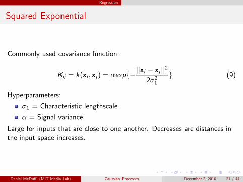
Squared Exponential
Commonly used covariance function:
Kij = k(xi , xj) = αexp{−||xi − xj ||
2
2σ21
} (9)
Hyperparameters:
σ1 = Characteristic lengthscale
α = Signal variance
Large for inputs that are close to one another. Decreases are distances inthe input space increases.
Daniel McDuff (MIT Media Lab) Gaussian Processes December 2, 2010 21 / 44
Regression
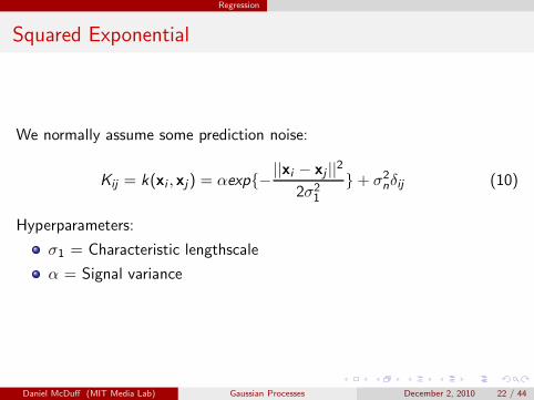
Squared Exponential
We normally assume some prediction noise:
Kij = k(xi , xj) = αexp{−||xi − xj ||
2
2σ21
}+ σ2nδij (10)
Hyperparameters:
σ1 = Characteristic lengthscale
α = Signal variance
Daniel McDuff (MIT Media Lab) Gaussian Processes December 2, 2010 22 / 44
Regression
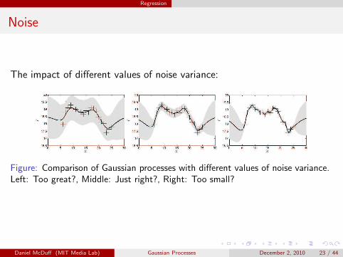
Noise
The impact of different values of noise variance:
Figure: Comparison of Gaussian processes with different values of noise variance.Left: Too great?, Middle: Just right?, Right: Too small?
Daniel McDuff (MIT Media Lab) Gaussian Processes December 2, 2010 23 / 44

Regression
Squared Exponential
We normally assume some prediction noise:
Kij = k(xi , xj) = αexp{−||xi − xj ||
2
2σ21
}+ σ2nδij (11)
Hyperparameters:
σ1 = Characteristic lengthscale
α = Signal variance
Daniel McDuff (MIT Media Lab) Gaussian Processes December 2, 2010 24 / 44
Regression
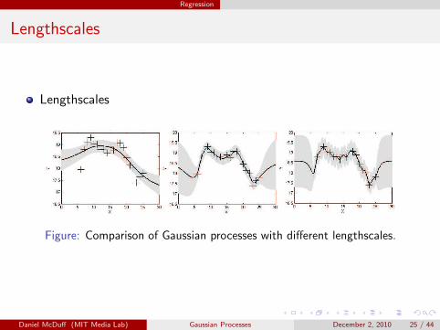
Lengthscales
Lengthscales
Figure: Comparison of Gaussian processes with different lengthscales.
Daniel McDuff (MIT Media Lab) Gaussian Processes December 2, 2010 25 / 44
Regression
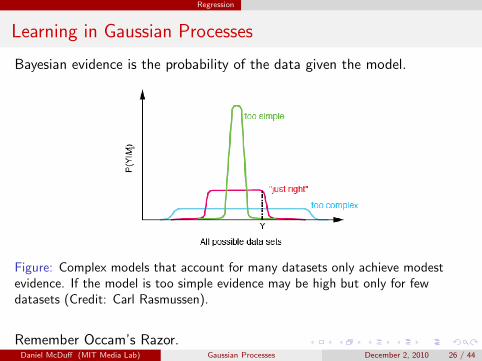
Learning in Gaussian Processes
Bayesian evidence is the probability of the data given the model.
Figure: Complex models that account for many datasets only achieve modestevidence. If the model is too simple evidence may be high but only for fewdatasets (Credit: Carl Rasmussen).
Remember Occam’s Razor.Daniel McDuff (MIT Media Lab) Gaussian Processes December 2, 2010 26 / 44
Regression
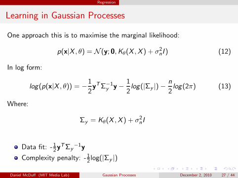
Learning in Gaussian Processes
One approach this is to maximise the marginal likelihood:
p(x|X , θ) = N (y;0,Kθ(X ,X ) + σ2nI ) (12)
In log form:
log(p(x|X , θ)) = −1
2yTΣ−1
y y−1
2log(|Σy |)−
n
2log(2π) (13)
Where:
Σy = Kθ(X ,X ) + σ2nI
Data fit: -12yTΣy
−1y
Complexity penalty: -12 log(|Σy |)
Daniel McDuff (MIT Media Lab) Gaussian Processes December 2, 2010 27 / 44
Regression
Learning in Gaussian Processes
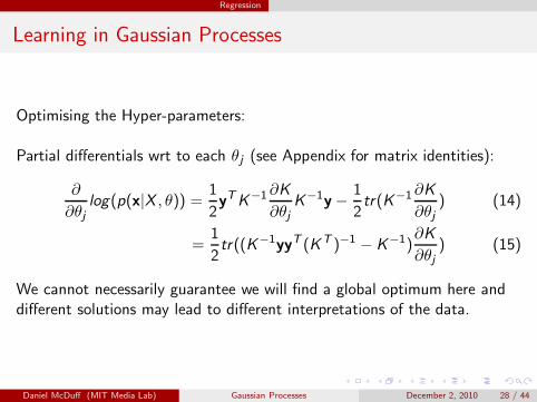
Optimising the Hyper-parameters:
Partial differentials wrt to each θj (see Appendix for matrix identities):
∂
∂θjlog(p(x|X , θ)) =
1
2yTK−1∂K
∂θjK−1y−
1
2tr(K−1∂K
∂θj) (14)
=1
2tr((K−1yyT (KT )−1 − K−1)
∂K
∂θj) (15)
We cannot necessarily guarantee we will find a global optimum here anddifferent solutions may lead to different interpretations of the data.
Daniel McDuff (MIT Media Lab) Gaussian Processes December 2, 2010 28 / 44
Regression
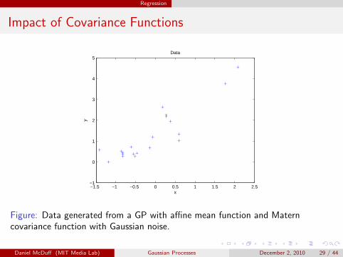
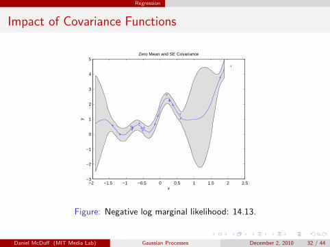
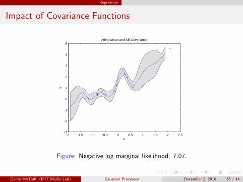
Impact of Covariance Functions
−1.5 −1 −0.5 0 0.5 1 1.5 2 2.5−1
0
1
2
3
4
5Data
x
y
Figure: Data generated from a GP with affine mean function and Materncovariance function with Gaussian noise.
Daniel McDuff (MIT Media Lab) Gaussian Processes December 2, 2010 29 / 44
Regression
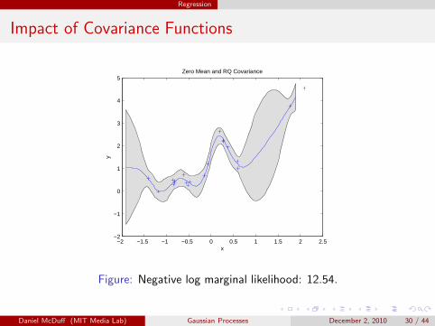
Impact of Covariance Functions
−2 −1.5 −1 −0.5 0 0.5 1 1.5 2 2.5−2
−1
0
1
2
3
4
5Zero Mean and RQ Covariance
x
y
Figure: Negative log marginal likelihood: 12.54.
Daniel McDuff (MIT Media Lab) Gaussian Processes December 2, 2010 30 / 44
Regression
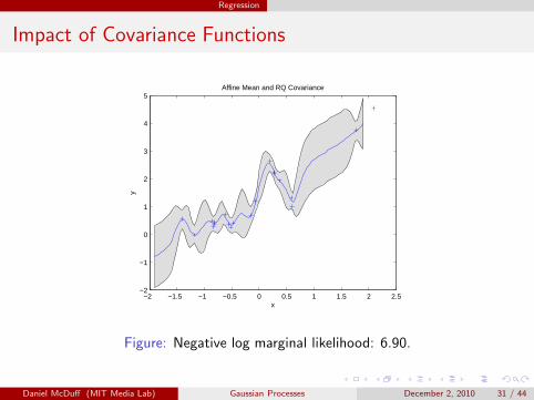
Impact of Covariance Functions
−2 −1.5 −1 −0.5 0 0.5 1 1.5 2 2.5−2
−1
0
1
2
3
4
5Affine Mean and RQ Covariance
x
y
Figure: Negative log marginal likelihood: 6.90.
Daniel McDuff (MIT Media Lab) Gaussian Processes December 2, 2010 31 / 44
Regression
Impact of Covariance Functions
−2 −1.5 −1 −0.5 0 0.5 1 1.5 2 2.5−3
−2
−1
0
1
2
3
4
5Zero Mean and SE Covariance
x
y
Figure: Negative log marginal likelihood: 14.13.
Daniel McDuff (MIT Media Lab) Gaussian Processes December 2, 2010 32 / 44
Regression
Impact of Covariance Functions
−2 −1.5 −1 −0.5 0 0.5 1 1.5 2 2.5−3
−2
−1
0
1
2
3
4
5Affine Mean and SE Covariance
x
y
Figure: Negative log marginal likelihood: 7.07.
Daniel McDuff (MIT Media Lab) Gaussian Processes December 2, 2010 33 / 44
Classification
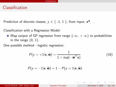
Classification
Prediction of discrete classes, y ∈ { -1, 1 }, from input, x*. .
Classification with a Regression Model:
Map output of GP regression from range {-∞, + ∞} to probabilitiesin the range {0, 1}.
One possible method - logistic regression:
P(y = +1|x, w) =1
1 + exp(−wTx)(16)
P(y = −1|x, w) = 1− P(y = 1|x, w)
Daniel McDuff (MIT Media Lab) Gaussian Processes December 2, 2010 34 / 44
Classification
Classification
There is a more general form of classification. We will not go into thedetails of this here. However, the concept is similar to the regression case.It once again involves marginalising over the model parameter distribution.
Unfortunately unlike the regression case there is not a simple analyticalsolution.
Daniel McDuff (MIT Media Lab) Gaussian Processes December 2, 2010 35 / 44
Classification
Classification
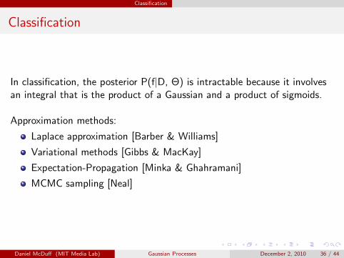
In classification, the posterior P(f|D, Θ) is intractable because it involvesan integral that is the product of a Gaussian and a product of sigmoids.
Approximation methods:
Laplace approximation [Barber & Williams]
Variational methods [Gibbs & MacKay]
Expectation-Propagation [Minka & Ghahramani]
MCMC sampling [Neal]
Daniel McDuff (MIT Media Lab) Gaussian Processes December 2, 2010 36 / 44
Classification
Complexity
The complexity of Gaussian processes is of the order N3, where N isthe number of data points, due to the inversion of the N x N matrix.
σ−2n (σ−2
n XXT +Σ−1p )−1 (17)
Daniel McDuff (MIT Media Lab) Gaussian Processes December 2, 2010 37 / 44
Applications
Applications
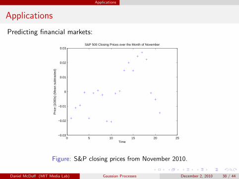
Predicting financial markets:
0 5 10 15 20 25−0.03
−0.02
−0.01
0
0.01
0.02
0.03S&P 500 Closing Prices over the Month of November
Time
Pric
e (1
000s
) (M
ean
subt
ract
ed)
Figure: S&P closing prices from November 2010.
Daniel McDuff (MIT Media Lab) Gaussian Processes December 2, 2010 38 / 44
Applications
Applications
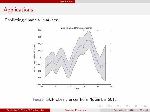
Predicting financial markets:
0 5 10 15 20 25−0.04
−0.03
−0.02
−0.01
0
0.01
0.02
0.03
0.04Zero Mean and Matern Covariance
Time
Pric
e (1
000s
) (M
ean
subt
ract
ed)
Figure: S&P closing prices from November 2010.
Daniel McDuff (MIT Media Lab) Gaussian Processes December 2, 2010 39 / 44
Applications
Applications
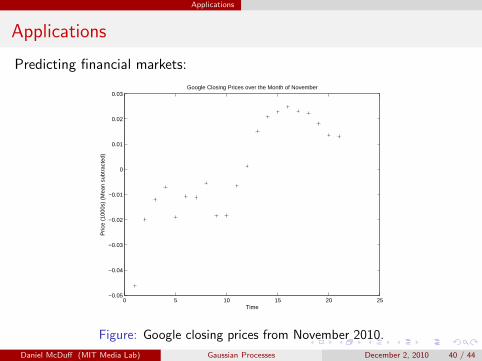
Predicting financial markets:
0 5 10 15 20 25−0.05
−0.04
−0.03
−0.02
−0.01
0
0.01
0.02
0.03Google Closing Prices over the Month of November
Time
Pric
e (1
000s
) (M
ean
subt
ract
ed)
Figure: Google closing prices from November 2010.
Daniel McDuff (MIT Media Lab) Gaussian Processes December 2, 2010 40 / 44
Applications
Applications
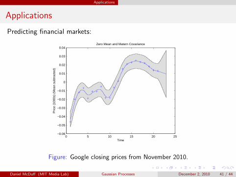
Predicting financial markets:
0 5 10 15 20 25−0.06
−0.05
−0.04
−0.03
−0.02
−0.01
0
0.01
0.02
0.03
0.04Zero Mean and Matern Covariance
Time
Pric
e (1
000s
) (M
ean
subt
ract
ed)
Figure: Google closing prices from November 2010.
Daniel McDuff (MIT Media Lab) Gaussian Processes December 2, 2010 41 / 44
Summary
Key Points
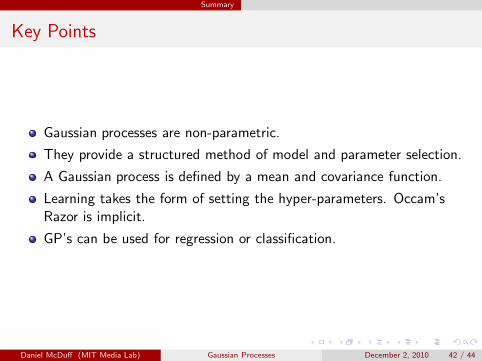
Gaussian processes are non-parametric.
They provide a structured method of model and parameter selection.
A Gaussian process is defined by a mean and covariance function.
Learning takes the form of setting the hyper-parameters. Occam’sRazor is implicit.
GP’s can be used for regression or classification.
Daniel McDuff (MIT Media Lab) Gaussian Processes December 2, 2010 42 / 44

Summary
Questions
Daniel McDuff (MIT Media Lab) Gaussian Processes December 2, 2010 43 / 44
Summary
Appendix
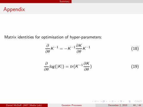
Matrix identities for optimisation of hyper-parameters:
∂
∂θK−1 = −K−1∂K
∂θK−1 (18)
∂
∂θlog(|K |) = tr(K−1 ∂K
∂θ) (19)
Daniel McDuff (MIT Media Lab) Gaussian Processes December 2, 2010 44 / 44
Recommended