Theoretical Computer Science 54 (1987) 87-102
North-Holland
87
GEOMETRIC OPTIMIZATION AND THE
POLYNOMIAL HIERARCHY *
Chanderjit BAJAJ
Department qf Computer Science, Purdue University, West Lafayette, IN 47907, U.S.A.
Abstract. We illustrate two techniques of accurately classifying the optimization versions of
geometric problems in the polynomial hierarchy. We show that if NPf Co-NP, then there are
interesting natural geometric optimization problems (location-allocation problems under minsum)
in A! that are in neither NP nor Co-NP. Hence, all these problems are shown to belong properly
to Al, the second level of the polynomial hierarchy. We also show that there are some interesting
geometric optimization problems (location-allocation problems under minmax) complete for a class D’ (which is contained in 3; and contains NPuCo-NP).
1. Introduction
Geometric optimization problems are inherently not pure combinatorial problems
since the optimal solution often belongs to an infinite feasible set, the entire real
(Euclidean) plane. Such geometric problems frequently arise in computer aided
geometric design and robotics and often naturally as optimization problems. It has
thus become increasingly important to devise appropriate methods to analyse the
complexity of geometric optimization problems and to classify them accurately in
the polynomial hierarchy. The adaptation of combinatorial analysis methods to
these inherently not pure combinatorial problems provides added significance.
Many of the geometric optimization problems such as the Euclidean Traveling
Salesman problem, the Euclidean Steiner Tree problem and the Euclidean Minimum
Spanning Tree problem can be thought of as special cases of well-studied graph
problems. Whereas the general problems deal with vertex points joined by edges
having arbitrarily specified lengths, the corresponding geometric problems deal with
points in the plane or in 3-space with the edge lengths being the actual interpoint
distances under one of the standard /,-metrics. Being special cases offers hope that
although these problems are difficult for arbitrary graphs (networks), efficient
algorithms could be possible for the corresponding geometric problems.
However, it is at times possible to show that the geometric cases of these problems
cannot be ‘any’ easier than the general problems, at least as far as the exact solution
is concerned. In the past, the recognition versions of the Euclidean Traveling
Salesman, Euclidean Steiner Tree problems [7] and certain geometric location
problems [l, 5, 13, 141, have been shown to be NP-complete. Also there are certain
* Supported in part by the National Science Foundation under Grant DC1 85.21356.
0304.3975/87/$3.50 @ 1987, Elsevier Science Publishers B.V. (North-Holland)
88 C. Bajaj
fundamental geometric optimization problems whose recognition versions are not
even known to be in the class NP and for some of these one can at times prove
that there exists no exact algorithm under various models of computation [2,3]. On
the other hand efficient polynomial time algorithms have been discovered for an
enormously large number of geometric optimization problems, [ 1, 171.
In this paper we consider a number of natural geometric optimization problems
in the plane and illustrate two techniques of accurately classifying their computa-
tional complexity. These problems arise as geometric reductions from various classes
of location-allocation optimization problems [4,6,9, lo] under standard I,-metrics
as well as more general arbitrary metrics. In Section 2, we show that if NP # Co-NP
then there are interesting natural geometric optimization problems (location-alloca-
tion problems under minsum) in A,’ that are in neither NP nor Co-NP. Hence, all
these problems are shown to belong properly to A ,‘, the second level of the polynomial
hierarchy. Next, in Section 3, we show that there are some interesting geometric
optimization problems (location-allocation problems under minmax) complete for
a class Dp. The class of Dp was defined in [15] as follows: L is in Dp iff L is an
intersection of L, and L2 such that L, is in NP and L, is in Co-NP. The class Dp
contains both NP and Co-NP and is contained in A:= PNP.
2. A ;-proper problems
We consider three different classes of geometric optimization problems derived
under a discrete minsum optimization criterion from certain location-allocation
problems in the Euclidean plane. A minsum location objective is one which mini-
mizes the sum of the costs resulting from a given location solution and is some
measure of the average cost of serving the destinations. Various applications have
been raised in the past under the discipline of location theory [6,9, lo]. A common
real-world example with a minsum objective that is cited there is one of locating a
water treatment plant so that the sum of the length of pipes required to serve water
to the various households or industrial users is minimized More recent examples
are those of locating components on a VLSI chip so as to minimize the sum of the
wire connections from the components or locating industrial robots so as to minimize
the sum of their respective distances from work bins.
Under this minsum location objective it is possible to distinguish two basic
approaches. The first suggests that location sites may be anywhere in the real
Euclidean plane, giving an infinite number of possible location sites. The second
approach considers only a finite number of known sites as feasible and models the
constraints imposed on the possible location, ensuring that undesirable and imprac-
tical locations need not be considered. The various distance metrics’ used, rectilinear
(I,), Euclidean (E,) and infinity (1,), reflect the appropriate problem restrictions.
’ Between two points a = (a,, a,) and h = (b,, h,) in the plane the I, distance is la, - h,l+ la, -b, 1;
the lz distance is ~‘(a, - b,)‘+(a, -b,,)’ and the & distance is max(la, - b,J, la! - b,I).
Geotnerric optimizaiion and the polynomial hierarch? 89
Given a set T = {(x,, y,) : i = 1, . . , n} of n fixed destination points (destinations)
in the real Euclidean plane and parameters k, m and L, we have the following
problems:
(0,):
(02):
(03):
Is L the minimum sum of the weighted distances of the n destinations and
the closest of the k locatable sources?
Is m the maximum number of destinations, m s n, for which the sum of the
weighted distances of these destinations from the closest of the k locatable
sources is 9 L?
Is k the minimum number of locatable sources for which the sum of the
weighted distances of the n destinations from the closest of these sources is
SL?
In the case of locating multiple sources as above, the allocation of the destinations
to the sources must also be ascertained. In the optimal solution each destination is
allocated to its closest located source. However, this optimal allocation is one of
the exceedingly large number of possible allocations.’ Not known a priori, it needs
to be determined. It is also interesting to note that the capacitated versions of these
geometric location-allocation optimization problems (with sources having finite
capacities) turn out to be various cases of the more familiar transportation-location
problems and, under discrete solution space constraints, to be the plant location
and warehouse location problems [6].
We show that the above optimization problems O’s under three different distance
metrics, I,, l2 and 1, as well as for feasible solution sets which are both finite and
injinite, all properly belong to the class A:, the second level of the polynomial
hierarchy. A problem L is a proper-d; problem if
(1) L is in A,‘;
(2) L is not in Xr= NP, assuming NP# Co-NP;
(3) L is not in II r = Co-NP, assuming NP # Co-NP.
Let problems P,, Pz and P3 correspond to the above problems which allow location
of the sources to be anywhere in the plane. Let problems Q, , Q2 and Q3 correspond
to problems P,, P2 and P3 respectively, with the location of the sources being
constrained to a finite discrete set S of possible locations in the plane and of size
polynomial in n. Further, let problems R,, R, and R, be restricted versions of
problems Qi, Q2 and Q3 respectively, with the locution of the sources being a subset
of T, the set of destination points.
To show that the above optimization problems are A!-proper, we first need to
show the corresponding recognition versions of these optimization problems to be
NP-complete. To show the recognition versions of the above optimization problems
to be NP-complete, we must formulate them in a more suitable manner. We assume
that the set of destination points T is given as a set of integer coordinate pairs.
Furthermore, we assume that the set T = {p, , . . , pn} is a multiset with w, points
in T with exactly the same coordinate p, conforming to a destination point p, having
’ The total number of possible assignments (allocations) of n destinations to k sources is S(n, k), the Stirling number of the 2nd kind.
90 C. Bajaj
an integer weight wj. From the optimization problems Pi, we obtain the corresponding
problems PP,.
Given the multiset T of destination points as specified before and integers k, m
and L, they are formulated thus:
(PP,) Is there a set KS={s,, . . , sk} of k sources in the plane such that the sum
of the distances between the destinations in T and the sources closest to them
1s SL?
(PP,) Is there a subset T’G T, 1 T’I 2 m, such that, for a set KS = {s,, . . . , sk} of k
sources in the plane, the sum of the distances between the destinations in T’
and the sources closest to them is <L?
(PP,) Is there a set KS, lKS\ s k, of sources in the plane such that the sum of the
distances between the destinations in T and the sources closest to them is c L?
One can also formulate the corresponding problems QQ and RR with the location
of sources restricted to finite sets, as specified before.
Lemma 2.1. PP, reduces to PP2. Further, PP, reduces to PPs. Similar results hold for
the problems QQ and problems RR.
Proof. PP, reduces to PP2, for T’= T and m = n. Further, PP, directly reduces to
PP3 since if less than k sources satisfy the limit L, k sources would definitely do
so. n
The discrete problem RR, was shown to be NP-complete for the (integerized)
Euclidean 1, distance metric in [14], where the integer value of the square root
radical of the /,-metric is considered. The decision problem under the &-metric
involves comparing the sums of square root radicals, a problem which is not even
known to be in NP. The algebraic difficulty of this is proved in [3]. Since the RR
problems are restricted versions of the corresponding QQ problems, it follows that
the finite solution space problem QQ, is also NP-complete for the l2 distance metric.
In [13], the infinite solution space problem PP, was shown to be NP-complete for
the 1, and integerized 1, distance metrics. We extend these results and show that for
the I, distance metric the infinite solution space problem PP, reduces to the corre-
sponding discrete RR, problem (and hence, to the finite solution space problem
QQ,) and thus these are all NP-complete. We complete the picture by showing that
the PP,, QQ, and RR, problems, for the I, distance metric are also NP-complete.
Using Lemma 2.1 it follows that the problems PP2, PP3 as well as the corresponding
problems QQ2, QQ3 and RR,, RR, are as difficult and also NP-complete for each
of the three distance metrics. The NP-completeness of the above problems implies
that the corresponding optimization problems, for both finite and infinite solution
spaces and for the three distance metrics, are all NP-hard. Assuming NP# Co-NP,
one can then show that each of the above optimization problems belong properly
in A,‘.
Geometric optimization and the polynomial hierarchy 91
The problems as formulated above are all in NP. We henceforth assume this fact
in all the NP-completeness proofs.
Theorem 2.2. Problem RR,, having a discrete feasible solution set, is NP-complete
for the I, distance metric.
Proof. To prove it complete we show a polynomial time reduction from the Exact
Cover problem, a known NP-complete problem [7]. The construction is similar to
the construction of [ 141 with a few essential changes to correspond to the 1, distance
metric. We repeat the enrire construction here for the sake of completeness and
also because of small typographical errors in the original.
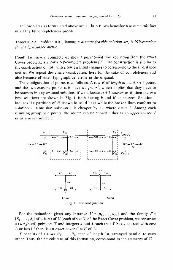
The configuration of points is as follows. A row R of length m has 6m + 4 points
and the two extreme points 6, b’ have weight m’, which implies that they have to
be sources in any optimal solution. If we allocate m + 2 sources to R, then the two
best solutions are shown in Fig. 1, both having b and b’ as sources. Solution 1
induces the partition of R shown in solid lines while the broken lines conform to
solution 2. Note that solution 1 is cheaper by 2~, where F = mp4. Among each
resulting group of 6 points, the source can be chosen either as an upper source s’
or as a lower source s.
b*c 1.5 1.5--1-b' --E
3.0 3.0
- +
. 3.0 l:.o . . 3.0 !“zo .
LOWIY UPPer
Fig. 1. Row configuration.
For the reduction, given any instance U = {u,, . . . , u,,} and the family F =
{S,, . . ., S,} of subsets of U (each of size 3) of the Exact Cover problem, we construct
a (weighted) point set T and integers k and L such that T has k sources with cost
L or less iff there is an exact cover Cc F of U.
T consists of t rows R,, . . . , R,, each of length 3n, arranged parallel to each
other. Thus, the 3n columns of this formation, correspond to the elements of U.
92 C. Bajaj
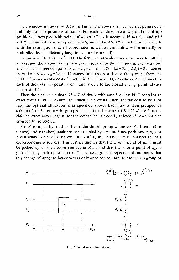
The window is shown in detail in Fig. 2. The spots x, y, w, z are not points of 7
but only possible positions of points. For each window, one of x, y and one of w, z
positions is occupied with points of weight n-‘; x is occupied iff ui +Z S,_, and y iff
u, E S,_, . Similarly w is occupied iff ui E S, and z iff U, g S,. (We use fractional weights
with the assumption that all coordinates as well as the limit L will eventually be
multiplied by a sufficiently large integer and rounded).
Define k = t(3n + 2) + 3n( t - 1). The first term provides enough sources for all the
t rows, and the second term provides one source for the q, q’ pair in each window.
L consists of three components L, + L, + L, . L, = t(2* 1.5+3n (12.2))-2ne comes
from the t rows. L2=3n( t - 1) comes from the cost due to the q or q’, from the
3n( t - 1) windows at a cost of 1 per pair. L, = 12n( t - I)/ n2 is the cost of connecting
each of the 6n( f- 1) points x or y and w or z to the closest q or q’ point, always
at a cost of 2.
Then there exists a subset KSc T of size k with cost L or less iff F contains an
exact cover C of U. Assume that such a KS exists. Then, for the cost to be L or
less, the optimal allocation is as specified above. Each row is then grouped by
solution 1 or 2. Let row Rj grouped as solution 1 mean that S, E C where C is the
claimed exact cover. Again, for the cost to be at most L, at least N rows must be
grouped by solution 1.
For R, grouped by solution 1 consider the ith group where u, E S,. Then both w
(above) and y (below) positions are occupied by a point. Since positions w, x, y or
z can charge only 2 to the cost in L3 of L, the w and y must connect to their
corresponding q sources. This further implies that the x or y point of qj_,,i must
be picked up by their lower sources in R,_,, and that the w of z point of q:,c is
picked up by their upper source. The same argument repeats and one notes that
this change of upper to lower occurs only once per column, where the ith group of
2.0 2.0
R2 1 L
X.. Y T
1 J .+3.0-t.~4+.+3.0+.
Pli-2.1 15 1.5
P!G+1,1
Fig. 2. Window configuration
Geometric optimization and the polynomial hierarchy 93
any row Rk, k <j, must have a lower source, while, for k > j, it must have an upper
source. Moreover, Rj causes the change to all three columns corresponding to the
three elements U, E S,. Also, there are no overlaps in the sets Sj of C since if U, E S,.,
then, by the crucial construction of the window, the positions w or y are 2 away
just from the solution-2 source (appropriate upper or lower), and if they are linked
up this way, this implies that R,. is grouped by solution 2, which means S,,a C.
Hence, C contains n sets without overlap and so is an exact cover.
Conversely, assume there is an exact cover C; then there exists a solution KS
having k sources of cost at most L, by allocating 3n +2 sources per row, 1 for each
9, q’ pair with R, grouped by solution 1 if S, E C and by solution 2 otherwise. Also,
for each (unique) S, E C and u, E S,, let the ith group of RI, for k 4 j have a lower
source and, for k>j, have an upper source, giving the total cost of L. 0
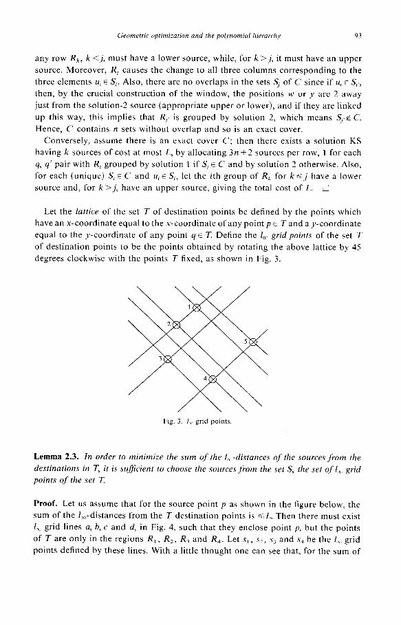
Let the lattice of the set T of destination points be defined by the points which
have an x-coordinate equal to the x-coordinate of any point p E T and a y-coordinate
equal to the y-coordinate of any point q E T. Define the I, grid points of the set T
of destination points to be the points obtained by rotating the above lattice by 45
degrees clockwise with the points T fixed, as shown in Fig. 3.
Fig. 3. I, grid points
Lemma 2.3. In order to minimize the sum of the lx-distances of the sources from the
destinations in T, it is suficient to choose the sources,from the set S, the set qf I, grid
points of the set T.
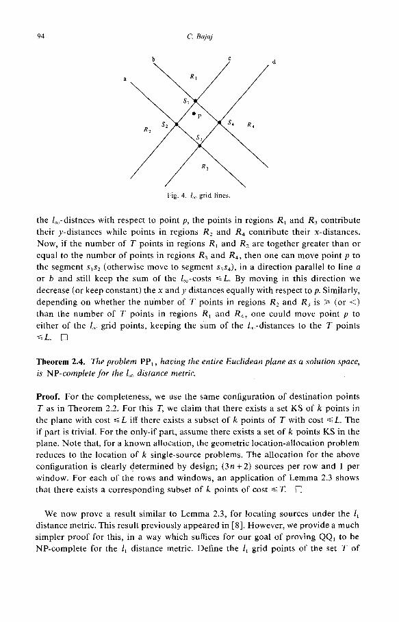
Proof. Let us assume that for the source point p as shown in the figure below, the
sum of the I,-distances from the T destination points is GL. Then there must exist
I, grid lines a, b, c and d, in Fig. 4, such that they enclose point p, but the points
of T are only in the regions R, , R2, R, and R,. Let s, , sz, sj and sq be the I, grid
points defined by these lines. With a little thought one can see that, for the sum of
94 C. Bajaj
Fig. 4. I, grid lines.
the l,-distnces with respect to point p, the points in regions R, and R3 contribute
their y-distances while points in regions R, and R, contribute their x-distances.
Now, if the number of T points in regions R, and Rz are together greater than or
equal to the number of points in regions R3 and R,, then one can move point p to
the segment s,s2 (otherwise move to segment s3s4), in a direction parallel to line a
or b and still keep the sum of the /,-costs sL. By moving in this direction we
decrease (or keep constant) the x and y distances equally with respect to p. Similarly,
depending on whether the number of T points in regions R2 and R3 is 2 (or <)
than the number of T points in regions R, and R,, one could move point p to
either of the 1, grid points, keeping the sum of the I,-distances to the T points
CL. 0
Theorem 2.4. The problem PP, , having the entire Euclidean plane as a solution space,
is NP-complete for the 1, distance metric.
Proof. For the completeness, we use the same configuration of destination points
T as in Theorem 2.2. For this T, we claim that there exists a set KS of k points in
the plane with cost s L iff there exists a subset of k points of T with cost G L. The
if part is trivial. For the only-if part, assume there exists a set of k points KS in the
plane. Note that, for a known allocation, the geometric location-allocation problem
reduces to the location of k single-source problems. The allocation for the above
configuration is clearly determined by design; (3n + 2) sources per row and 1 per
window. For each of the rows and windows, an application of Lemma 2.3 shows
that there exists a corresponding subset of k points of cost s T. q
We now prove a result similar to Lemma 2.3, for locating sources under the 1,
distance metric. This result previously appeared in [ 81. However, we provide a much
simpler proof for this, in a way which suffices for our goal of proving QQ, to be
NP-complete for the 1, distance metric. Define the 1, grid points of the set T of
Geometric optimization and the polynomial hierarchy 95
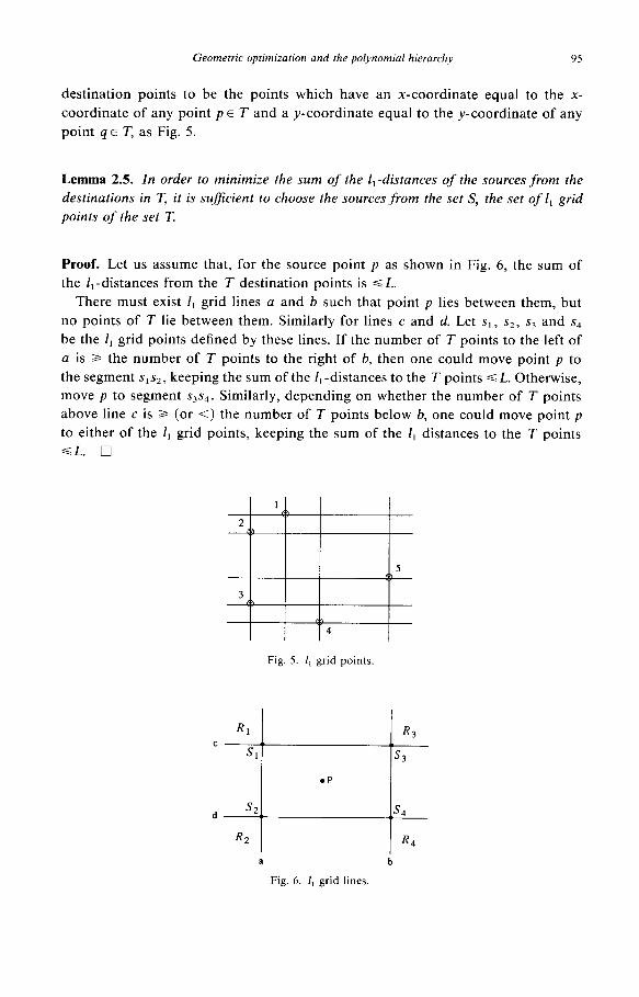
destination points to be the points which have an x-coordinate equal to the x-
coordinate of any point p E T and a y-coordinate equal to the y-coordinate of any
point q E T, as Fig. 5.
Lemma 2.5. In order to minimize the sum of the l,-distances of the sources from the
destinations in T, it is su$icient to choose the sources from the set S, the set of 1, grid
points of the set T.
Proof. Let us assume that, for the source point p as shown in Fig. 6, the sum of
the II-distances from the T destination points is GL.
There must exist I, grid lines a and 6 such that point p lies between them, but
no points of T lie between them. Similarly for lines c and d. Let s,, s2, s3 and s4
be the E, grid points defined by these lines. If the number of T points to the left of
a is 2 the number of T points to the right of b, then one could move point p to
the segment s1s2, keeping the sum of the I, -distances to the T points G L. Otherwise,
move p to segment s3s4. Similarly, depending on whether the number of T points
above line c is > (or <) the number of T points below 6, one could move point p
to either of the I, grid points, keeping the sum of the 1, distances to the T points
SL. 0
Fig. 5. I, grid points.
RI R3 c
Sl s3
l P
d s2. “S4
R2 R4
a b
Fig. 6. I, grid lines.
96 C. Bajaj
Theorem 2.6. The discrete solution space problems RRi and QQi for the 1, distance
metric are all NP-complete.
Proof. The infinite solution space problem PP, was shown to be NP-complete for
the 1, distance metric in [13]. A simple reduction from this problem to the discrete
solution space problem RR, can be obtained by letting the destination set T’ of
RR, to be the 1, grid points of the discrete set PP, . The proof of Lemma 2.5 suffices
to show that there exists a solution for RR, iff there exists a solution for PP, The
NP-completeness of QQ, again follows automatically from the NP-completeness of
the RR, problem. 0
Theorem 2.7. All the problems PP,, QQ, and RR,, for each of the three distance metrics
(I,, l2 and I,), are strongly NP-complete.
Proof. The magnitude of the largest number occurring in any instance I of the
problems PP, (similar for QQI and RR,) for the 1, distance metric is determined
by either the coordinate pairs of the destination set T or by the parameters k, m or
L. The parameters k and m are both integer values less than n. The constructions
in Theorem 2.2 and Lemma 2.3 show the strong NP-completeness of PP, , QQ, and
RR, since what has been exhibited is a bounded polynomial transformation from
Exact Cover (a strong NP-complete problem [7]). The lengths of the two problems
are polynomially related and are polynomials in n. Further, the function (the
iff-reduction mapping) is polynomial time computable. The integer coordinate pairs
of the points of T are bounded by O(n) and the value of L can be seen to be
bounded by 0( n’). Hence, the maximum value occurring in the construction of the
geometric location-allocation problems is bounded by a polynomial in n and hence,
bounded by a polynomial in the maximum value and length of an instance of the
Exact Cover problem.
The reduction of [ 131 for the NP-completeness of problem PP, for the I,- and
II-distances, is a bounded transformation from 3-Sat (strongly NP-complete [7])
and hence, the strong NP-completeness for these problems follows as above. The
strong completeness of the problems QQ, and RR, for the I,-metric (Theorem 2.6)
and for the /,-metric [14] follows again from their transformation from the Exact
Cover problem.
The problems PP2 and PP, (similarly for the corresponding QQ and RR problems)
have m and k respectively as their decision parameters and are actually number
problems, and consequently, strongly NP-complete. The strong completeness of
these problems also follows from the direct transformation from the above PP,
problems (Lemma 2.1). 0
To show that our optimization problems 0, are AI-proper for infinite, finite and
discrete solution sets, we use techniques first developed in [12] for combinatorial
optimization problems. We show that it applies to our case of geometric optimization
Geometric optimization and the polynomial hierarch) 97
problems based on our choice of decision problems and on the strong NP-complete-
ness result of Theorem 2.7. In the following, let Length[ I] be a measure for the size
of the instance Z of the problem, and Max[ Z] be the magnitude of the largest number
occurring in the instance I. For our problems we have Length [I] = some polynomial
in n, where n is the number of given destination points.
Lemma 2.8. The optimization problems 0, are in 3;.
Proof. A problem P is in 6; if P if; (Turing reduces to) Q, where Q is in NP. For
each of the Oi, where the sources are located in the entire plane, a Turing reduction
exists to the corresponding NP-complete recognition version PPi. For those 0,‘s
where the sources are located on a discrete set S or on the set of destination points
T, the corresponding NP-complete versions QQI and RR, are used respectively. For
0,) the value of parameter L in any instance I of the problem lies in the range 0 to cLen&tll f. r some constant c. By a simple binary search one can find the optimum
value of L in at most log cLength”’ = O(Length[Z]) calls of the PP, oracle. Since
Length[Z] is some polynomial in n, the reduction is polynomial time bound. For
problems O2 and O3 with their respective parameters m and k, the parameter values
range from 1 to n and so a sequential search suffices. 0
Each of the problems O;, where the sources are located in the entire plane, is the
optimization version of the corresponding NP-complete problem PP,. Then the
complement of PP,, PPT is a Co-NP-complete problem.
Lemma 2.9. Zf NP # Co-NP, then the optimization problems 0, are not in NP.
Proof. For each of the 0,‘s a nondeterministic polynomial time many-one reduction
[ll] (a,“’ ) guesses the optimal value of the parameter q (L for 0, , m for 0, and
k for 0,), uses the Oi oracle to verify that q is the optimum and then checks to see
if it is worse than the input q’ to PPi. Worse is either less or greater, depending on
whether 0, is a maximum or a minimum optimization problem. This shows that
PP’;s;p 0,. Then, as GE’ preserves the class of NP, it follows that Oi E NP implies
PP: E NP which is impossible if NP # Co-NP since PPj is NP-complete. 0
Lemma 2.10. Zj” NP # Co-NP, then the optimization problems Oi are not in Co-NP.
Proof. For each 0,, the fact that the corresponding PP, problem is strongly NP-
complete guarantees that PP~GF OL;, where <,’ IS a polynomial time positive reduc-
tion [ 1 l] which requires at most Max[ I] ‘yes’ answers of the 0: oracle to answer
any instance Z of PPY. This is so since Max[Z] G some polynomial in n (because
of strong NP-completeness, Theorem 2.7). (For those Oi where the sources are
located on a discrete set S or on the set of destination points T, the corresponding
NP-complete versions QQ, and RR, are used respectively, in place of PPP). Now,
98 C. Bajaj
Oi E Co-NP iff 0: E NP. But S ,’ p reserves the class of NP and it follows that 0: E NP
implies PPY E NP, which is impossible if NP # Co-NP since PP, is NP-complete. 0
The proof of the theorem below follows from the above and from Lemmas 2.8,
2.9 and 2.10.
Theorem 2.11. The geometric location-allocation optimization problems under minsum
for each of the three distance metrics as well as for infinite and$nite and discrete feasible
solution sets are all Al-proper, assuming NP# Co-NP.
3. DP-complete problems
We now consider geometric optimization problems derived under a discrete
minmax optimization criterion from location-allocation problems. A minmax loca-
tion objective is one which minimizes the maximum cost resulting from a given
location solution. Various applications have been raised in facility-location theory
[6,9, lo], where there exists sufficient justification in minimizing the effects of the
worst situation. A common real-world situation that might be formulated with a
minmax objective is one of locating health clinics so that the maximum distance a
patient must travel to a clinic is minimized. Another example concerns the placement
of fire stations in a large metropolitan area such that the maximum distance between
any location within the city and the nearest fire station is minimized.
Given the set T, as specified before, of n destinations in the plane, we formulate
the following problems:
(P,) Locate k points (sources) so as to minimize the maximum of the weighted
distances between the destinations and the sources closest to them;
(P2) Locate k points (sources) so that for a maximum number of destinations the
weighted distances of these destinations from their closest sources does not
exceed a prescribed limit R;
(PJ Locate a minimum number of points (sources) so that the maximum of the
weighted distances of the destinations and their closest sources does not exceed
a prescribed limit R;
However, in the following problems we assume that all weights are equal (similar
to assuming that wj = 1, for j = 1, . . , n) and show that even for this restricted case
the above problems are quite difficult.
Under the minmax criterion with Euclidean 1, distance metric, each of the above
location-allocation optimization problems reduces in a direct fashion to the place-
ment of equal-radius circular disks (circles) on the plane, with the centers of the
circles corresponding to the location of the sources. (For the 1, and 1, metric the
problems reduce to the placement of squares in the plane with two different
orientations). Further, all the destinations covered by the same circle correspond
also in a direct fashion to an allocation of these destinations to the source (the
center of the circle). Having equal weights for the above problems results in equally
Geometric optimization and the polynomial hierarchy 99
sized circles. Considering each of the above problems P, for equally sized circles,
which we call problems PCi, we show that each of these problems are complete for
the complexity class Dp.
The geometric optimization problems turn out to be simple optimization questions
concerning the size and number of geometric objects and are the natural questions
that one may ask when dealing with the packing and covering of such geometrical
objects. Initially versed in terms of circles, the proofs generalize to other geometric
figures in the plane corresponding to the different distance metrics. In the following,
denote the real Euclidean plane by E2 and a circle locatable anywhere in E2 to
mean that the center of the circle can be any point in the Euclidean plane. Further-
more, let an R-circle be a circle of radius R. Then given a set T = {(xi, y,) : i = 1, . . . , n}
of n fixed points in the real Euclidean plane and integers k and m, the set of
optimization problems are as follows
(PC,) Is R the minimum radius’ of k equally sized circles locatable anywhere in
E2 to cover the n points of T?
( PC2) Is m (m s n) the maximum number of points of T that k R-circles locatable
anywhere in E2 can cover?
(PC,) Is k the minimum number of R-circles locatable anywhere in E2 to cover the
n points of T?
We now show all the above geometric optimization problems to be complete for
the complexity class Dp. We first show that the problem PC3 of locating the minimum
number of R-circles in E2 to cover all the n demand points is DP-complete by
reducing (Sat, UnSat), a known DP-complete problem [15], to it. To show member-
ship in Dp, we use the fact that Dp can be defined as the class of all predicates
R(x) that can be expressed as
R(x) = PY P(x, ~11 A Wz Q(x, ~11
for some polynomial balanced and polynomial time checkable P and Q. Next we
show the remaining problems to be DP-complete by a similar reduction or a series
of polynomial time reductions.
In [16], it is proved that, similar to polynomial time many-one reductions,
polynomial time positive reductions preserve the class NP. That is, if a language
L, polynomial time positive reduces (or polynomial time many-one reduces) to a
language L,, then L2~ NPJ L, E NP. A similar fact is true for the class Co-NP.
Therefore, these positive reductions are adequate to separate the class of Dp-
complete languages from the classes of NP and Co-NP (assuming NP # Co-NP).
Thus, in our proofs, we may use both many-one and positive polynomial time
reductions. It is important to note that polynomial time Turing reductions which
do not preserve the class NP are not adequate in separating Dp languages from NP
and Co-NP. Thus, for instance, it is possible to polynomial time Turing reduce the
DP-complete language (Sat, UnSat) to (Sat), a known NP-complete problem. Also
3 Here R is considered as an integer-valued parameter. The problem appears to be DK-hard when R
is a real-valued parameter.
note that the special case of disjunctive, conjunctive positive reductions which we
use here are by far the strongest of the various other positive and truth-table
reducibilities known [lo]. In turn, any truth-table reduction is stronger than a Turing
reduction.
Theorem 3.1. The problem PC3 of locating the minimum number of R-circles in E2 to
cover the n given points is Dp complete.
Proof. The problem is in DP since it can be rephrased as the conjunction of a
predicate in NP and a predicate in Co-NP: (3(p,, . . , pk) E E2)[R-circles with
centers at p, , . . . , pk cover n points] A (V(q,, . . . , qk_,) E E’)[R-circles with centers
at ql,..., qkPl cover <n points].
To prove the completeness we reduce (Sat, UnSat) to PC3, using polynomial time
positive reductions. Starting from (F, , F2) and adapting a polynomial time construc-
tion in [5], we construct two separate sets of points S, and S2 in the plane such
that, for i = 1,2, exactly k, R-circles are required to cover all the n, points in Si if
F, is satisfiable. Further, if F, is not satisfiable, at least ki+ 1 and at most k, + c,
R-circles are needed to cover all the n, points of Si, where c, is the number of
clauses in the CNF formula F,.
Now, construct c2 additional copies of the set of points S, . We now have (c,+ 1)
copies of sets of points S, and a single set of points S2. (The reader may wish to
see for himself why (c,+ 1) copies of S, are required.) Let n = (c,+ l)n, + nz. It is
not hard to see that k, the minimum number of circles of radius R needed to cover
all the n points, satisfies
(cZ+l)k,+kz+1~k~(cz+l)k,+k2+cZ
iff F, is satisfiable and Fz is not satisfiable. Since this is a disjunction of at most c2
calls of PC3, problem PC3 is DP-complete under a polynomial time positive (disjunc-
tive) reduction from (Sat, UnSat). 0
Corollary 3.2. The problem PC2 of locating k R-circles in E2 to cover a maximum
number of the given points is D’-complete.
Proof. The problem is in Dp since it can be rephrased, as before, as the conjunction
of a predicate in NP and a predicate in Co-NP: (3(p,, . . , pk) E E2)[R-circles with
centers at pI, . . . , pk cover m points] A (V(q,, . . . , qk) E E’)[R-circles with centers
at q,,... , qk cover Sm points].
To prove the completeness we again reduce (Sat, UnSat) to PC3, using polynomial
time positive (disjunctive) reductions in a way very similar to Theorem 3.1. 0
Theorem 3.3. 7’he problem PC, of locating k equally sized circles of minimum radius
to cover all the n given points is DP-complete.
Proof. The problem is in Dp when R is an integer parameter since it can be rephrased,
as before, as the conjunction of a predicate in NP and a predicate in Co-NP:
Geometric optimization and the polynomial hierarch) 101
(3(p,, . . . , pk) E E*)[R-circles with centers at p,, . . . ,pk cover n points] A
(Vq, 9 . . . 9 qk) E E*)[(R - 1)-circles with centers at q,, . . . , qk cover <n points].
To prove it complete we show that PC3 polynomial time positive reduces to PC,.
We construct a set S of the radii of all possible circles which minimally cover n
points in the plane. Since the minimum enclosing circle for a set of points is defined
by exactly two or three of the points, the total size of S is at most (i)+(_y) which
is O(n’). We claim that k is the minimum number of R-circles that cover all n
points iff, for some s E S, s s R, s is the minimum radius of k circles to cover all n
points and, for some s E S, s > R, s is the minimum radius of k - 1 circles to cover
all n points. The proof is straightforward and follows from the definitions of the
two problems PC, and PC. Again, since we have a conjunction of two sets of
disjunctive calls of PC, (at most O(n’) calls), we have a polynomial time positive
reduction from PC3 to PC,. 17
4. Conclusion
There are a number of interesting open issues. First, is there a natural geometric
optimization problem which is A_:-proper? This has been a persistent open problem
in the context of combinatorial optimization. A problem Q is proper for A! if Q is
in AS and not in Xl or II:‘, assuming X;f # TII. Second, exhibit many-one reductions
for the proofs of D”-completeness. Another open question is the precise complexity
of the unique versions of the above geometric optimization problems.
5. References
[I] C. Bajaj, Geometric optimization and computational complexity, Ph.D. Thesis, Tech. Report
TR84-629, Computer Science Dept., Cornell University, 1984. [2] C. Bajaj, Proving geometric algorithm non-solvability: an application of factoring algorithms, J.
Symbolic Comput. 2 (1986) 99-102.
[3] C. Bajaj, Limitations to algorithmic solvability: Galois methods and models of computation, in:
Proc. ACM Svnp. on Symbolic and Algebraic Computation (1986) 71-16.
[4] L. Cooper, Location-allocation problems, Oper. Res. ll(3) (1963) 331-343.
[5] R. Fowler, M. Paterson and S. Tanimoto, Optimal packing and covering in the plane are NP-
complete, In.form. Process. Left. lZ(3) (1981) 133-137.
[6] R. Francis and J. White, Facility Layout and Location-an Analytic Approach (Prentice Hall,
Englewood Cliffs, NJ, 1974). [7] M. Carey and D. Johnson, Computers and Intractability: A Guide to NP-completeness (Freeman,
San Francisco, 1979).
[8] P. Hansen, J. Perreur and J. Thisse, Location theory, dominance and convexity: some further results,
Oper. Res. 28 (1980) 1241-1250.
[9] G. Handler and P. Mirchandani, Location on Networks Theory and Algorithms (MIT Press, Cambridge, MA, 1979).
[lo] J. Krarup and P. Pruzan, Selected families of discrete location problems, Ann. Discrete Math. 5
(1979) 327-387.
102 C. Bajaj
[ 1 l] R. Lndner, N. Lynch and A. Selman, Comparison ofpolynomial time reducibilities, Theoret. Comput.
Sci. 1 (1975) 103-123. [12] E.W. Leggett and D.J. Moore, Optimization problems and the polynomial hierarchy, Theoret.
Comput. Sci. 15 (1981) 279-289.
[ 131 N. Megiddo and K.J. Supowit, On the complexity of some common geometric location problems,
SIAMJ. Comput. 13(l) (1984) 182-196.
[14] C. Papadimitriou, Worst-case and probabilistic analysis of a geometric location problem, SIAM J.
Comput. lO(3) (1981) 542-557.
[15] C. Papadimitriou and M. Yannakakis, The complexity of facets (and some facets of complexity), J. Comput. System Sci. 28 (1984) 244-259.
[16] A.L. Selman, Analogues of semirecursive sets and effective reducibilities to the study of NP-
completeness, Inform. and Control 52 (1982) 36-51.
[17] M.I. Shamos, Computational geometry, Ph.D. Thesis, Yale University, 1978.
Recommended