Investigating Movement Patterns of Prime Bull African Elephants in the
Associated Private Nature Reserves of Kruger National Park,
South Africa
Patrick Freeman and Lucia Herrero
Abstract
Partnering with Save the Elephants-South Africa, one of the premier elephant research and
conservation organizations in Southern Africa, we will be mapping and analyzing the
movements of ten adult, large-tusked bull elephants throughout the network of private reserves
that link directly into the great Kruger National Park in South Africa. Understanding the
movements of these high-profile, high-risk animals in this protected area network is integral to
the successful management of elephant populations in this transboundary ecosystem.
Background and Context According to the World Wildlife Fund, the African savannah elephant is a threatened species,
still recovering from decimating levels of hunting during the 1970s and 1980s. Elephants are a
critical factor in maintaining ecosystem health because of their large-scale interactions with their
environment. Often referred to as “ecosystem engineers,” elephants can greatly alter their
surroundings as they browse on trees, disperse seeds from those trees across, and clear forest
habitat to make way for more open grasslands. Thus, they can also be seen as a keystone species,
supporting a broad network of other wildlife species, both plant and animal. Because elephants
require such a large range, they face habitat loss and population fragmentation with increasing
land development, a problem that is gripping most of the regions that make up the African
elephant’s current range.
Additionally, elephants are also in the throes of extremely high rates of illegal hunting to fuel a
burgeoning demand for ivory products in the Far East, namely China, with estimates of total
losses to the total African elephant population summing to somewhere near 35,000 elephants per
year. Cynthia Moss, one of the world’s foremost elephant researchers, has said that if poaching
rates continue at present levels we may be living in a world without wild African elephants
within the next two decades (Stein, 2012).
Most of these losses have been sustained in East Africa, however, and elephant populations in
Southern Africa are actually on the increase in many range-states. While this is good news, there
are significant challenges associated with maintaining high elephant densities within established
protected areas, primarily dealing with the over-exploitation of bounded ecosystems by highly
destructive elephant feeding. There is also growing worry that the poaching activity that has been
largely contained to the East and Central African range states will spread into the protected
strongholds in southern Africa. Thus, research into elephant ecology in these regions is both
timely and necessary for the continuing successful management of this incredibly important
species.
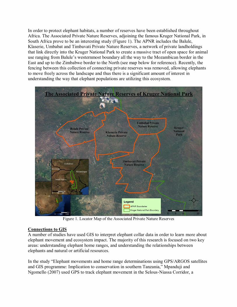
In order to protect elephant habitats, a number of reserves have been established throughout
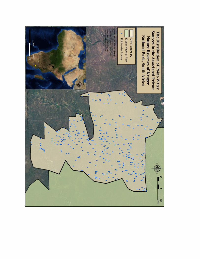
Africa. The Associated Private Nature Reserves, adjoining the famous Kruger National Park, in
South Africa prove to be an interesting study (Figure 1). The APNR includes the Balule,
Klaserie, Umbabat and Timbavati Private Nature Reserves, a network of private landholdings
that link directly into the Kruger National Park to create a massive tract of open space for animal
use ranging from Balule’s westernmost boundary all the way to the Mozambican border in the
East and up to the Zimbabwe border to the North (see map below for reference). Recently, the
fencing between this collection of connecting private reserves was removed, allowing elephants
to move freely across the landscape and thus there is a significant amount of interest in
understanding the way that elephant populations are utilizing this ecosystem.
Figure 1. Locator Map of the Associated Private Nature Reserves
Connections to GIS
A number of studies have used GIS to interpret elephant collar data in order to learn more about
elephant movement and ecosystem impact. The majority of this research is focused on two key
areas: understanding elephant home ranges, and understanding the relationships between
elephants and natural or artificial resources.
In the study “Elephant movements and home range determinations using GPS/ARGOS satellites
and GIS programme: Implication to conservation in southern Tanzania,” Mpanduji and
Ngomello (2007) used GPS to track elephant movement in the Selous‐Niassa Corridor, a
protected area which spreads through Tanzania and Mozambique, and links two important
wildlife reserves, Selous and Niassa. A GIS spatial analysis revealed that a significant subset of
the elephant population in the Selous-Niassa area had large home ranges—that is, they were
highly mobile and regularly traveled within the full extent of the Corridor. Furthermore, the GIS
analysis shows that the large home range elephants relied on the Selous-Niassa Corridor to safely
travel between the two main reserves (Mpanduji and Ngomello 2007). This suggests that it is of
vital importance to protect these lands in order for elephants to maintain their traditional
lifeways.
In addition, two studies have attempted to quantify the relationship between elephant movement
and the distribution of water sources. In “Do artificial waterholes influence the way herbivores
use the landscape? Herbivore distribution patterns around rivers and artificial surface water
sources in a large African savanna park” Smit et al. (2007) tested if soil type, water source type
(natural or artificial), and water source availability influenced the migratory patterns of large
herbivores, including elephants. Using GIS, Smit et al. (2007) performed a density analysis to
determine that artificial waterholes significantly influenced the way large herbivores are
distributed within a given area.
These findings are supported by the study “Fences and artificial water affect African savannah
elephant movement patterns.” In this study, Loarie et al. (2009) attempt to understand how
artificial water sources and fences affect elephant movements. Using data acquired from GPS
tracking system, Loarie et al. (2009) used GIS and an ANOVA analysis to analyze migratory
patterns according to seasonality. They determined that human intervention, via artificial fencing
and water sources, reduces seasonal differences in elephant movement (Loarie et al. 2009). In
turn, they suggest that reduced migration creates the possibility for elephants to overexploit
resources (Loarie et al. 2009).
These studies raise critical questions about ethical and responsible conservation—at what point
does human interaction become helpful or potentially harmful? They serve as a guide for the
kinds of questions that will motivate this project, and provide methods that may prove fruitful in
the analysis.
Study Objectives It is our objective to better understand how the elephants residing within the APNR occupy this
space and interact with their environment. In order to achieve this, we have collaborated with
Save the Elephants-South Africa (STE-SA) to answer these questions. STE-SA is one of the
leading elephant research and conservation organizations currently operating in Southern Africa.
STE-SA has been running a strong elephant collaring operation since the early 2000s in order to
obtain vital information on the movements and spatial ecology of elephants that move
throughout the transboundary ecosystems of the APNR and Kruger National Park.
Using the GPS collaring data points collected by STE-SA, we aim to develop a methodology for
answering the following questions:
Objective 1: Understanding Elephant Movements Do individuals exhibit a preference for parts of their range, or are their movements evenly
dispersed over the entirety of this reserve network? Are there hot-spots of activity? Do these hot-
spots shift in response to changes in seasons? Additionally, for those individuals that have
several years’ worth of data collected, do general trends in spatial utilization illustrate shifts over
time or are they relatively constant?
Objective 2: Understanding Relationships between Clusters and the Environment
Are there any discernible relationships between the proximity of clustered elephant movements
to certain vegetation types and to the nearest point-water source? If so, can these relationships be
used to establish a model to predict where elephants might spend the majority of their time?
Projected Coordinate System for Project For our analysis, we will be utilizing the Universal Transverse Mercator projected coordinate
system. Our study area falls completely within Zone 36S of the Universal Transverse Mercator
grid and over a relatively small amount area, thus minimizing distortion when data is projected.
Therefore, our analysis that calculates distance and area will be rigorous and minimally distorted.
Thematic Layers to be Used in Analysis
Elephant GPS Collar Data:
Data Type: Vector, points
Source: Save the Elephants – South Africa sponsored GPS collars
Original Coordinate System: WGS1984
Projected Coordinate System: Tete UTM – Zone 36S
Time Period: Data provided was highly variable both temporally and in volume. Some
individuals had many years of consecutive data from their collars while others only had several
months and much fewer points.
As stated above, STE-SA has engaged in an intensive elephant-collaring operation since the
early 2000s in an effort to understand the spatial ecology of the elephant populations that
frequent the Kruger National Park-Greater Kruger transboundary ecosystem that includes the
APNR. While the organization has long kept a photographic database that catalogues observed
individuals within the Greater Kruger ecosystem, the tracking of individual movements has been
an incredibly powerful conservation tool that allows us to understand how these animals utilize
the space available to them as well as continue to advocate for their protection. Large bull
elephants, given both their prodigious appetites and prime breeding status can range over large
tracts of the landscape in the search for resources and mating opportunities. Knowing this, STE-
SA’s ongoing campaign to track the movements of large, senior bulls in this ecosystem has
yielded large amounts of data regarding the usage of space by several individuals. STE-SA has
provided the raw GPS collar data for a total of 10 individual elephants designated as prime bulls
within the APNR. These males are considered to be of prime breeding age and potential and thus
represent a very important demographic to the continuing health of elephant populations in this
reserve network. Additionally, senior bulls act as repositories of ecological knowledge and thus
when serving as mentors to young bulls, can transfer this knowledge accordingly, making them
of particular interest within the context of social behavior studies.
Once an individual has been collared, their geographic coordinates are relayed to a satellite using
a specified data capture regime (e.g. four times per day; this variable also varied across
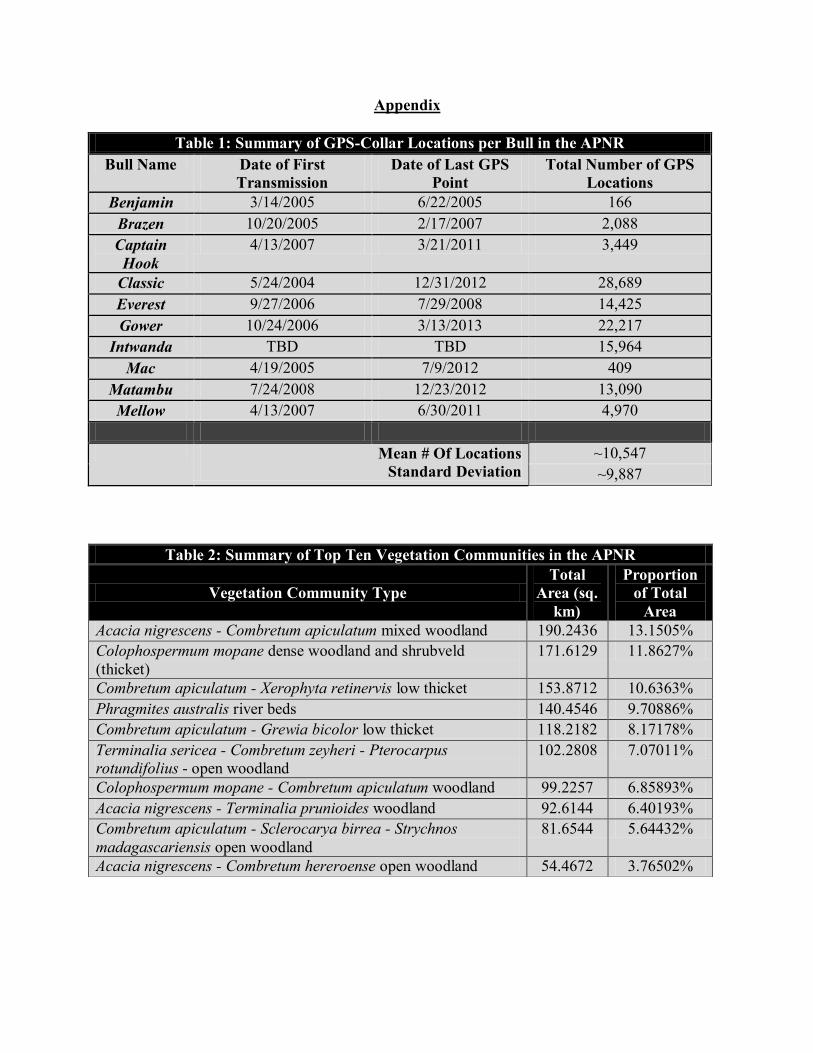
individuals) for compilation in a database. A summary table of the total number of GPS locations
for each animal has been included in Table 1 in the Appendix for review. Total GPS location
records range from 166 to over 30,000 and records per individual and span ranges of several
months to several years. It is important to mention that not all of these bulls were collared at the
same time nor were they all from the same social group. Instead, they are collared when (a)
resources can be obtained to purchase a collar and arrange for the darting of the animal to outfit
it with a collar and (b) when the animal is accessible for darting.
Additionally, the data provided to us has been clipped to the APNR boundaries despite there
being no boundaries between the APNR and the adjoining Kruger National Park because our
analysis focuses solely on the space utilization of these bulls within the APNR. As much of this
GPS collar research is still under active development determining the ideal number of GPS
locations to relay per day is still being tested. As such, data for each individual varies in this
characteristic and steps are being taken to sort the data to determine the data collection regime
for each animal. Information about this variance can be found in the summary tables in the
Appendix. These facts will be taken into account during analysis to produce the most informative
and statistically sound results possible.
This layer will be used in a hot-spot and cold-spot analysis of the density of elephant locations
across the landscape. More details about this analysis can be found in the Methodology Outline
section. This dataset will also be used in the linear regression model to determine the relationship
between the location of these bulls and other factors like the distance to the nearest point-water
source and vegetation type.
Vegetation Community Data:
Data Type: Vector, polygons
Source: Save the Elephants – South Africa in conjunction with ecological monitoring teams in
Timbavati, Klasserie, and Umbabat Private Nature Reserves
Date of Collection: Unknown
Original Coordinate System: Assumed to be WGS1984
Projected Coordinate System: Tete UTM – Zone 36S
STE-SA has also provided us with data on the dominant vegetation communities present in this
network of reserves. Unfortunately only the vegetation communities in Umbabat, Timbavati, and
Klasserie Private Nature Reserves have been mapped to date. In total there are 24 different
classes of vegetation that have been mapped. Vegetation polygons were generated through a
field-based plant sample collection and ground-truthing with a GPS. While the overarching
ecosystem present in the APNR falls under the dry woodland savanna label, there are multiple
variations in the vegetative make-up of this landscape. A table of the top ten most prevalent
vegetation communities has been provided in the Appendix (Table 2). The vegetation
community that makes up the most area in the reserve is the Acacia nigrescens (knobthorn) –
Combretum apiculatum (red bush willow) open woodland, with a total of around 13% of the total
area of the reserve being occupied by this dominant vegetation. The second most prevalent
community in the APNR is the Colophospermum mopane dense woodland and shrubveld,
making up just over 11% of the total area of the APNR. It is of note that all of these species of
tree are heavily exploited by elephants and thus we investigated whether or not our study
individuals are choosing to occupy areas dominated by these vegetation communities through the
use of our regression model.
Water Points:
Data Type: Vector, points
Source: Save the Elephants – South Africa in communication with regional ecological
monitoring teams
Date of Collection: Up-to-date as of 2012
Original Coordinate System: WGS1984
Projected Coordinate System: Tete UTM – Zone 36S
STE-SA has provided us with GIS layers for all of the point-water sources in the APNR as well
as the layers for some of the rivers in the region. These data were collected with the help of the
ecological monitoring teams of each reserve and mapped using a GPS waypoint and sent to us
via ESRI shapefiles. A map of these point water sources is included in the Appendix. In total
there are 364 point-water sources within the boundaries of the three major reserves that make up
the APNR that we also have vegetation data for (Klasserie, Umbabat, and Timbavati Private
Nature Reserves). Elephant movements in a similar ecosystem to that found in the APNR have
been shown to be heavily influenced by water availability (Loarie, et al. 2009) and thus it is
important to understand how this particular elephant demographic is influenced by this variable
within this tightly transboundary ecosystem. We will be employing these point-water source
locations to build our regression model to determine if there are any relational trends between the
movement of these bulls and their relative distance to the nearest water source.
Methodologies
Pre-Analysis Data Preparation of GPS-Collar Data:
Original elephant GPS collar data was delivered as a database for each individual not separated
by year or season. Thus, we created a new feature class for each individual for each year (i.e.
Classic_2007) where entire datasets existed (qualified as those datasets that have points collected
from January 1 to December 31 of each year).
We then went on to break those individuals for which we have complete annual data sets into
seasonal datasets. The seasons in this region can be broadly classified into wet and dry and are
characterized by their relative levels of precipitation. According to the Kruger National Park’s
Web site, the wet season runs from October to March and the dry season runs from April to
September (“Kruger National Park”). Thus we separated our GPS-collar data into these
categories to investigate any rudimentary changes in distribution of bull movements. As entire
wet seasons are not contained within a single year and instead traverse two calendar years, we
generated data using points from October through December of the previous year and points
from January to March for the newyear to create an entire seasonal set where possible. We
acknowledge that in reality seasonality is not discrete in nature, however to test the functionality
of this analysis we utilize this assumption. This parameter can of course be changed in the future
as necessary.
Please see Appendix for full Model Builder Flowcharts.
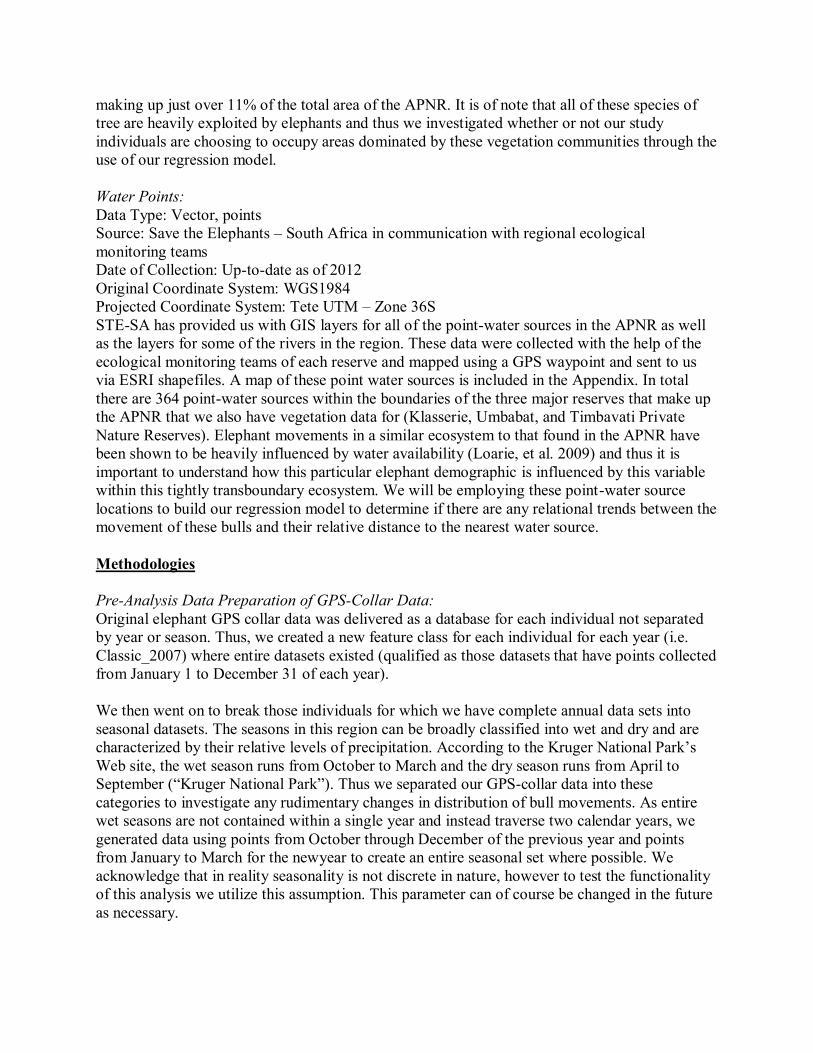
Understanding General Distribution Patterns
In order to understand the general spatial distribution of an
individual’s total range within any given year or season,
the Mean Center and Standard Deviation Ellipse tools were
employed. For the Standard Deviation Ellipse Tool, two
standard deviations were selected to incorporate 95% of the
locations, excluding 5% with the aim of excluding outliers
from the dataset. This basic tool can track subtle changes
in the mean center of each individual’s range as well as the
dispersal of points across their range both annually and
seasonally.
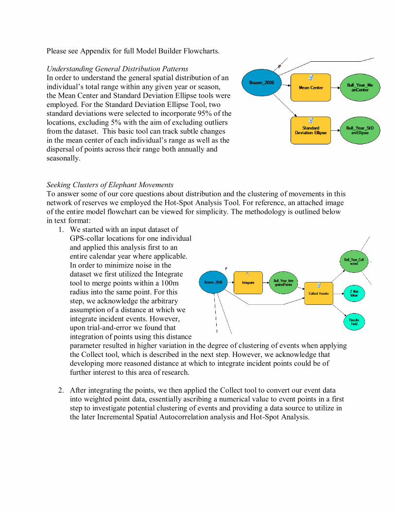
Seeking Clusters of Elephant Movements
To answer some of our core questions about distribution and the clustering of movements in this
network of reserves we employed the Hot-Spot Analysis Tool. For reference, an attached image
of the entire model flowchart can be viewed for simplicity. The methodology is outlined below
in text format:
1. We started with an input dataset of
GPS-collar locations for one individual
and applied this analysis first to an
entire calendar year where applicable.
In order to minimize noise in the
dataset we first utilized the Integrate
tool to merge points within a 100m
radius into the same point. For this
step, we acknowledge the arbitrary
assumption of a distance at which we
integrate incident events. However,
upon trial-and-error we found that
integration of points using this distance
parameter resulted in higher variation in the degree of clustering of events when applying
the Collect tool, which is described in the next step. However, we acknowledge that
developing more reasoned distance at which to integrate incident points could be of
further interest to this area of research.
2. After integrating the points, we then applied the Collect tool to convert our event data
into weighted point data, essentially ascribing a numerical value to event points in a first
step to investigate potential clustering of events and providing a data source to utilize in
the later Incremental Spatial Autocorrelation analysis and Hot-Spot Analysis.
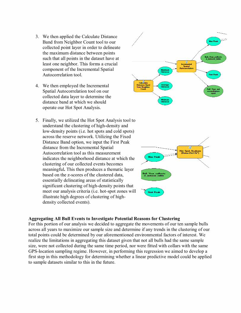
3. We then applied the Calculate Distance
Band from Neighbor Count tool to our
collected point layer in order to delineate
the maximum distance between points
such that all points in the dataset have at
least one neighbor. This forms a crucial
component of the Incremental Spatial
Autocorrelation tool.
4. We then employed the Incremental
Spatial Autocorrelation tool on our
collected data layer to determine the
distance band at which we should
operate our Hot Spot Analysis.
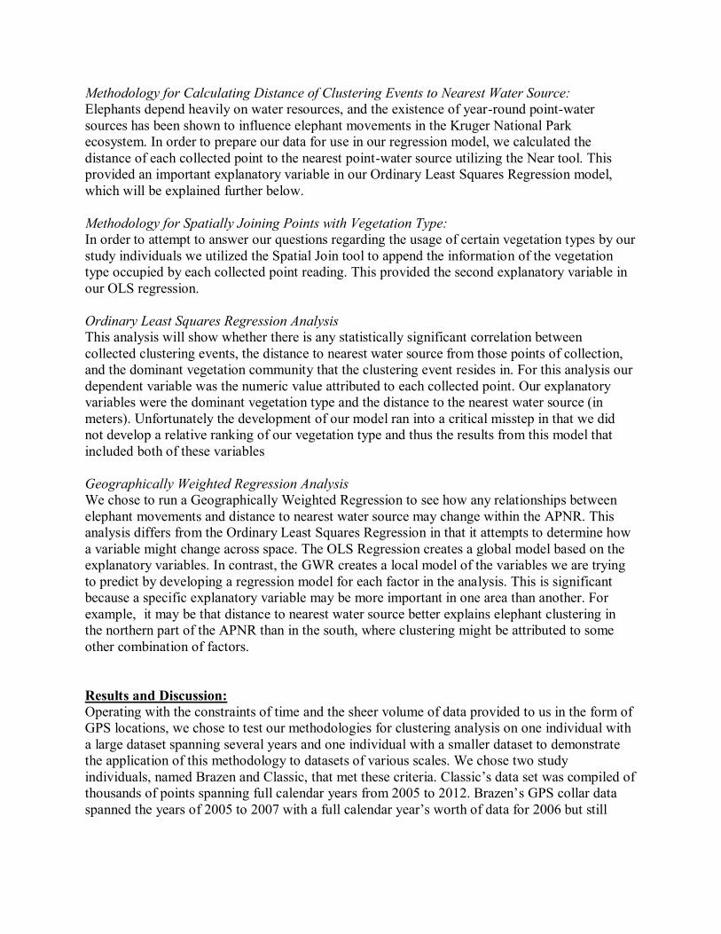
5. Finally, we utilized the Hot Spot Analysis tool to
understand the clustering of high-density and
low-density points (i.e. hot spots and cold spots)
across the reserve network. Utilizing the Fixed
Distance Band option, we input the First Peak
distance from the Incremental Spatial
Autocorrelation tool as this measurement
indicates the neighborhood distance at which the
clustering of our collected events becomes
meaningful. This then produces a thematic layer
based on the z-scores of the clustered data,
essentially delineating areas of statistically
significant clustering of high-density points that
meet our analysis criteria (i.e. hot-spot zones will
illustrate high degrees of clustering of high-
density collected events).
Aggregating All Bull Events to Investigate Potential Reasons for Clustering For this portion of our analysis we decided to aggregate the movements of our ten sample bulls
across all years to maximize our sample size and determine if any trends in the clustering of our
total points could be determined by our aforementioned environmental factors of interest. We
realize the limitations in aggregating this dataset given that not all bulls had the same sample
size, were not collected during the same time period, nor were fitted with collars with the same
GPS-location sampling regime. However, in performing this regression we aimed to develop a
first step in this methodology for determining whether a linear predictive model could be applied
to sample datasets similar to this in the future.
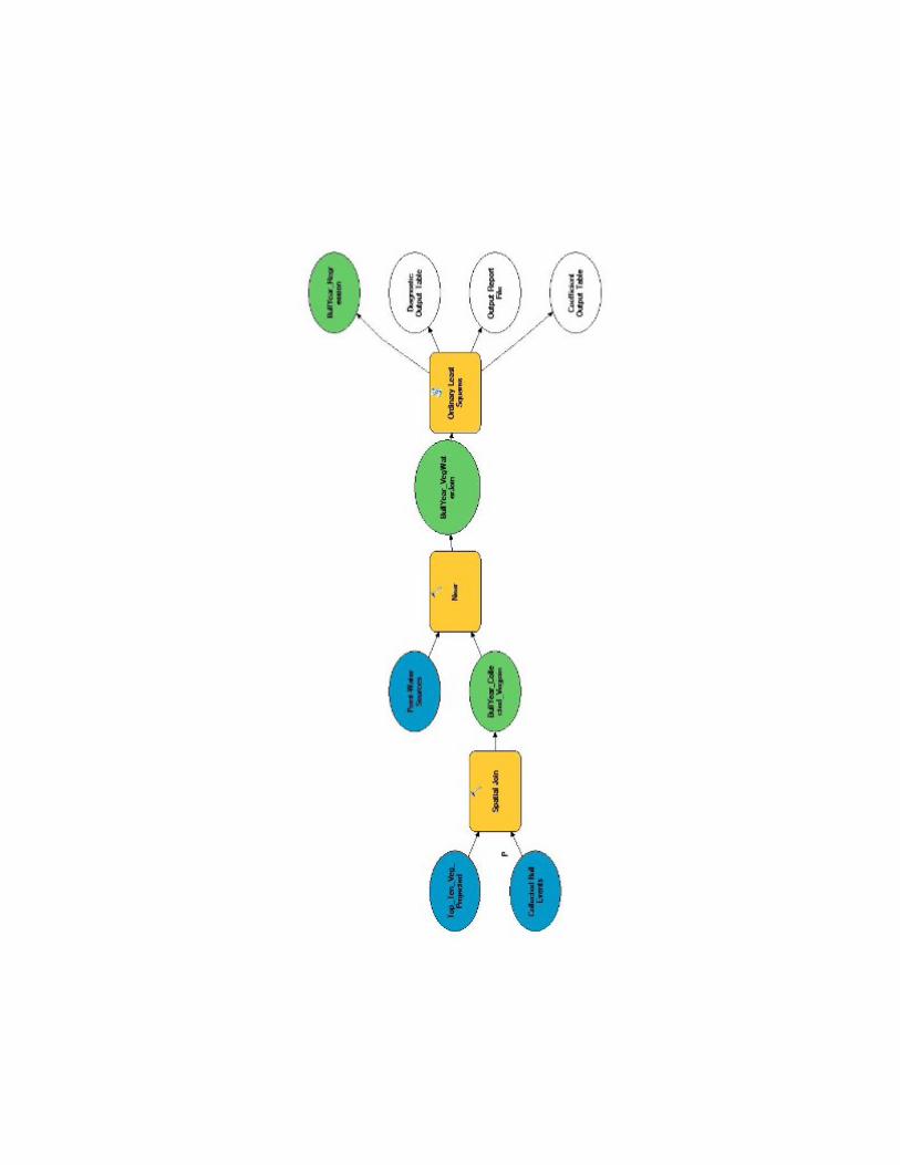
Methodology for Calculating Distance of Clustering Events to Nearest Water Source:
Elephants depend heavily on water resources, and the existence of year-round point-water
sources has been shown to influence elephant movements in the Kruger National Park
ecosystem. In order to prepare our data for use in our regression model, we calculated the
distance of each collected point to the nearest point-water source utilizing the Near tool. This
provided an important explanatory variable in our Ordinary Least Squares Regression model,
which will be explained further below.
Methodology for Spatially Joining Points with Vegetation Type:
In order to attempt to answer our questions regarding the usage of certain vegetation types by our
study individuals we utilized the Spatial Join tool to append the information of the vegetation
type occupied by each collected point reading. This provided the second explanatory variable in
our OLS regression.
Ordinary Least Squares Regression Analysis
This analysis will show whether there is any statistically significant correlation between
collected clustering events, the distance to nearest water source from those points of collection,
and the dominant vegetation community that the clustering event resides in. For this analysis our
dependent variable was the numeric value attributed to each collected point. Our explanatory
variables were the dominant vegetation type and the distance to the nearest water source (in
meters). Unfortunately the development of our model ran into a critical misstep in that we did
not develop a relative ranking of our vegetation type and thus the results from this model that
included both of these variables
Geographically Weighted Regression Analysis
We chose to run a Geographically Weighted Regression to see how any relationships between
elephant movements and distance to nearest water source may change within the APNR. This
analysis differs from the Ordinary Least Squares Regression in that it attempts to determine how
a variable might change across space. The OLS Regression creates a global model based on the
explanatory variables. In contrast, the GWR creates a local model of the variables we are trying
to predict by developing a regression model for each factor in the analysis. This is significant
because a specific explanatory variable may be more important in one area than another. For
example, it may be that distance to nearest water source better explains elephant clustering in
the northern part of the APNR than in the south, where clustering might be attributed to some
other combination of factors.
Results and Discussion:
Operating with the constraints of time and the sheer volume of data provided to us in the form of
GPS locations, we chose to test our methodologies for clustering analysis on one individual with
a large dataset spanning several years and one individual with a smaller dataset to demonstrate
the application of this methodology to datasets of various scales. We chose two study
individuals, named Brazen and Classic, that met these criteria. Classic’s data set was compiled of
thousands of points spanning full calendar years from 2005 to 2012. Brazen’s GPS collar data
spanned the years of 2005 to 2007 with a full calendar year’s worth of data for 2006 but still
encompassing one complete set of wet season months and one complete set of dry seasons
events.
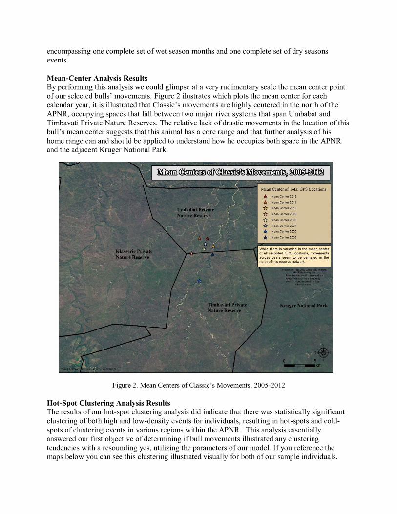
Mean-Center Analysis Results
By performing this analysis we could glimpse at a very rudimentary scale the mean center point
of our selected bulls’ movements. Figure 2 ilustrates which plots the mean center for each
calendar year, it is illustrated that Classic’s movements are highly centered in the north of the
APNR, occupying spaces that fall between two major river systems that span Umbabat and
Timbavati Private Nature Reserves. The relative lack of drastic movements in the location of this
bull’s mean center suggests that this animal has a core range and that further analysis of his
home range can and should be applied to understand how he occupies both space in the APNR
and the adjacent Kruger National Park.
Figure 2. Mean Centers of Classic’s Movements, 2005-2012
Hot-Spot Clustering Analysis Results
The results of our hot-spot clustering analysis did indicate that there was statistically significant
clustering of both high and low-density events for individuals, resulting in hot-spots and cold-
spots of clustering events in various regions within the APNR. This analysis essentially
answered our first objective of determining if bull movements illustrated any clustering
tendencies with a resounding yes, utilizing the parameters of our model. If you reference the
maps below you can see this clustering illustrated visually for both of our sample individuals,
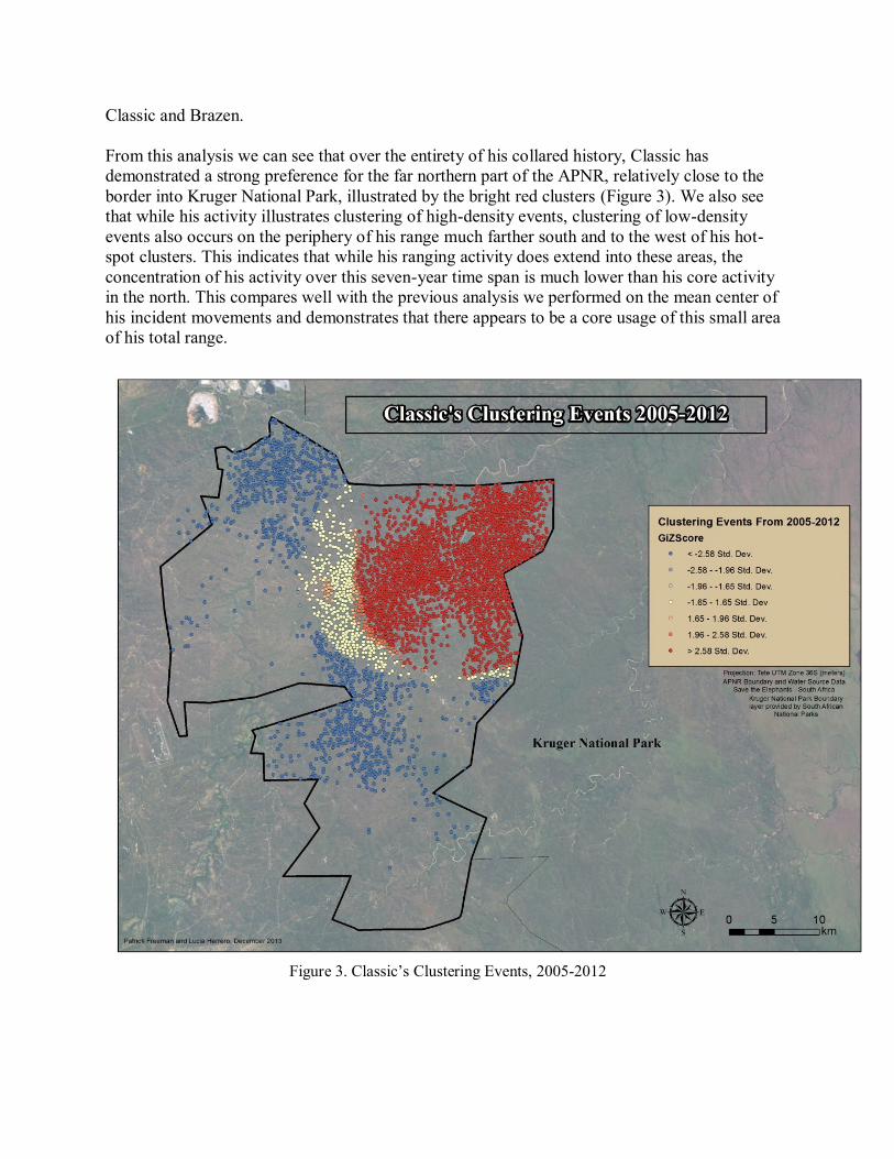
Classic and Brazen.
From this analysis we can see that over the entirety of his collared history, Classic has
demonstrated a strong preference for the far northern part of the APNR, relatively close to the
border into Kruger National Park, illustrated by the bright red clusters (Figure 3). We also see
that while his activity illustrates clustering of high-density events, clustering of low-density
events also occurs on the periphery of his range much farther south and to the west of his hot-
spot clusters. This indicates that while his ranging activity does extend into these areas, the
concentration of his activity over this seven-year time span is much lower than his core activity
in the north. This compares well with the previous analysis we performed on the mean center of
his incident movements and demonstrates that there appears to be a core usage of this small area
of his total range.
Figure 3. Classic’s Clustering Events, 2005-2012
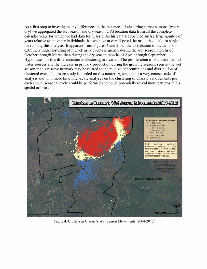
As a first step to investigate any differences in the instances of clustering across seasons (wet v.
dry) we aggregated the wet season and dry season GPS location data from all the complete
calendar years for which we had data for Classic. As his data set spanned such a large number of
years relative to the other individuals that we have at our disposal, he made the ideal test subject
for running this analysis. It apparent from Figures 4 and 5 that the distribution of incidents of
extremely high clustering of high-density events is greater during the wet season months of
October through March than during the dry season months of April through September.
Hypotheses for this differentiation in clustering are varied. The proliferation of abundant natural
water sources and the increase in primary production during the growing seasons seen in the wet
season in this reserve network may be related to the relative concentrations and distribution of
clustered events but more study is needed on this matter. Again, this is a very coarse scale of
analysis and with more time finer-scale analyses on the clustering of Classic’s movements per
each annual seasonal cycle could be performed and could potentially reveal more patterns in his
spatial utilization.
Figure 4. Clusters in Classic’s Wet Season Movements, 2004-2012
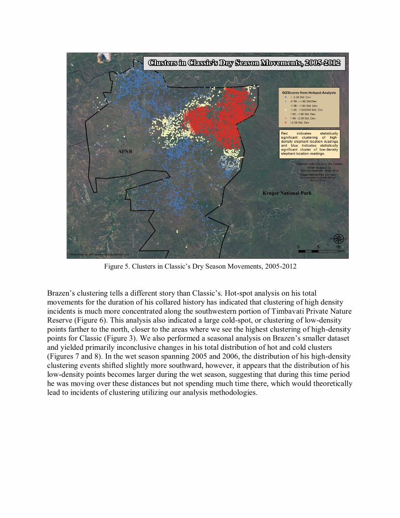
Figure 5. Clusters in Classic’s Dry Season Movements, 2005-2012
Brazen’s clustering tells a different story than Classic’s. Hot-spot analysis on his total
movements for the duration of his collared history has indicated that clustering of high density
incidents is much more concentrated along the southwestern portion of Timbavati Private Nature
Reserve (Figure 6). This analysis also indicated a large cold-spot, or clustering of low-density
points farther to the north, closer to the areas where we see the highest clustering of high-density
points for Classic (Figure 3). We also performed a seasonal analysis on Brazen’s smaller dataset
and yielded primarily inconclusive changes in his total distribution of hot and cold clusters
(Figures 7 and 8). In the wet season spanning 2005 and 2006, the distribution of his high-density
clustering events shifted slightly more southward, however, it appears that the distribution of his
low-density points becomes larger during the wet season, suggesting that during this time period
he was moving over these distances but not spending much time there, which would theoretically
lead to incidents of clustering utilizing our analysis methodologies.
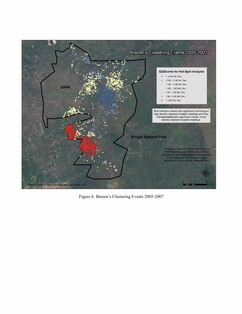
Figure 6. Brazen’s Clustering Events 2005-2007
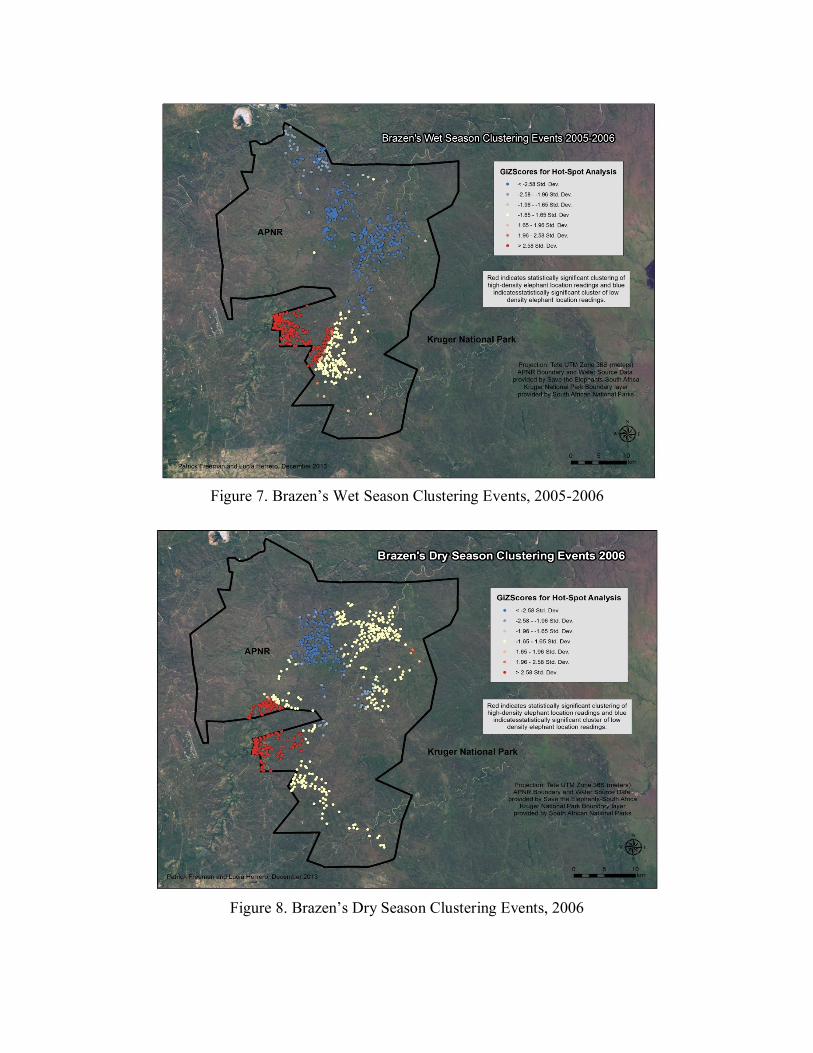
Figure 7. Brazen’s Wet Season Clustering Events, 2005-2006
Figure 8. Brazen’s Dry Season Clustering Events, 2006
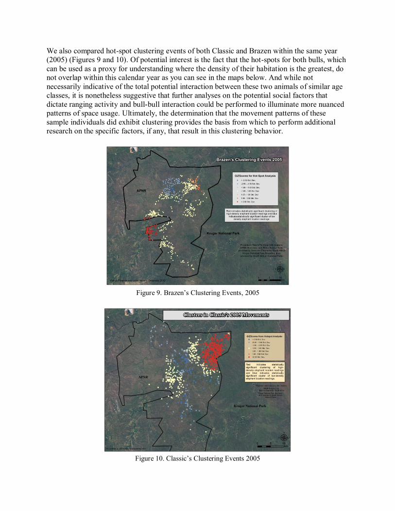
We also compared hot-spot clustering events of both Classic and Brazen within the same year
(2005) (Figures 9 and 10). Of potential interest is the fact that the hot-spots for both bulls, which
can be used as a proxy for understanding where the density of their habitation is the greatest, do
not overlap within this calendar year as you can see in the maps below. And while not
necessarily indicative of the total potential interaction between these two animals of similar age
classes, it is nonetheless suggestive that further analyses on the potential social factors that
dictate ranging activity and bull-bull interaction could be performed to illuminate more nuanced
patterns of space usage. Ultimately, the determination that the movement patterns of these
sample individuals did exhibit clustering provides the basis from which to perform additional
research on the specific factors, if any, that result in this clustering behavior.
Figure 9. Brazen’s Clustering Events, 2005
Figure 10. Classic’s Clustering Events 2005
Linear Regression Results In addition to understanding how elephant movements are distributed throughout the APNR, we
were also interested in trying to describe the motivating factors behind these movements. We
hypothesize that the elephant’s environment plays a large role in determining where an elephant
tends to cluster. With this in mind, we hoped to establish a predictive model using the total
collected points for all prime bulls, the corresponding vegetation type, and the distance to nearest
water source to better understand why elephant clustering occurs. Furthermore, we hope to
establish a methodology for using Ordinary Least Squares Regression and Geographically
Weighted Regression for future studies of elephant movements.
Ordinary Least Squares Regression Results
In the OLS, we set the weighted average location (ICOUNT, from collected points) as the
dependent variable and the vegetation types and distance to nearest water source as the
explanatory variables. The OLS resulted in an adjusted r2 value of .03. This suggests that the
location of approximately three percent of the clustered points can be explained by the kind of
vegetation the point is associated with and how far that point is from water. Based on what we
know about elephant resource dependency, we find this value to be very low.
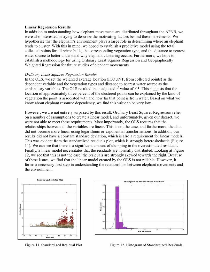
However, we are not entirely surprised by this result. Ordinary Least Squares Regression relies
on a number of assumptions to create a linear model, and unfortunately, given our dataset, we
were not able to meet these requirements. Most importantly, the OLS requires that the
relationships between all the variables are linear. This is not the case, and furthermore, the data
did not become more linear using logarithmic or exponential transformations. In addition, our
results did not have a constant standard deviation, which is also a requirement for linear models.
This was evident from the standardized residuals plot, which is strongly heteroskedastic (Figure
11). We can see that there is a significant amount of clumping in the overestimated residuals.
Finally, a linear model necessitates that the residuals are normally distributed. Looking at Figure
12, we see that this is not the case; the residuals are strongly skewed towards the right. Because
of these issues, we find that the linear model created by the OLS is not reliable. However, it
forms a necessary first step in understanding the relationships between elephant movements and
the environment.
Figure 11. Standardized Residual Plot Figure 12. Histogram of Standardized Residuals
Geographically Weighted Regression Results
In addition to the OLS, we also performed a Geographically Weighted Regression. The GWR is
significant because it takes into account spatial variation by creating a linear model for each
variable at the local level. Thus, the GWR will allow us to see how the relationship between
elephant clustering and distance to nearest water source varies across the APNR.
For this GWR, we set the weighted average location (ICOUNT, from collected points) of the
total bulls as the dependent variable and the calculated distance to nearest point-water source as
the explanatory variable. The GWR resulted in an adjusted r2 value of .54. This means that the
location of approximately fifty-four percent of the clustered points can be explained how far they
are from the nearest point-water source. This adjusted r2 value is quite significant, and it is
exciting that such a strong correlation can be drawn between elephant clustering and the presence
of water.
However, the Geographically Weighted Regression is still a linear model and is therefore subject
to all the assumptions required for the Ordinary Least Squares Regression. Because of this, we
find that our model is unreliable. In addition to this, the Akaike Information Criterion (AIC) for
the GWR was 72,000. This lends considerable doubt to the accuracy of our findings. Finally, in
order for the GWR to be as accurate as possible, it requires that all of the explanatory variables
are included. Since we only had an accurate data set for artificial point-water source locations,
we could not include a number of interesting other variables that may help explain elephant
clustering, like the vegetation type, distance to natural water sources, like rivers and seasonal
drainages, and distance to human infrastructures, like roads, settlements, and park boundaries.
Therefore, it is likely that the GWR has over-attributed significance to distance to artificial point-
water sources, because it was unable to account for any other explanatory variables.
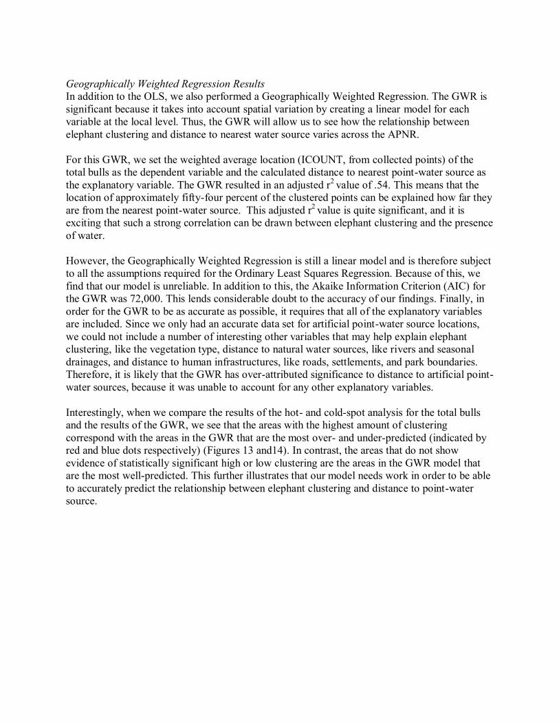
Interestingly, when we compare the results of the hot- and cold-spot analysis for the total bulls
and the results of the GWR, we see that the areas with the highest amount of clustering
correspond with the areas in the GWR that are the most over- and under-predicted (indicated by
red and blue dots respectively) (Figures 13 and14). In contrast, the areas that do not show
evidence of statistically significant high or low clustering are the areas in the GWR model that
are the most well-predicted. This further illustrates that our model needs work in order to be able
to accurately predict the relationship between elephant clustering and distance to point-water
source.
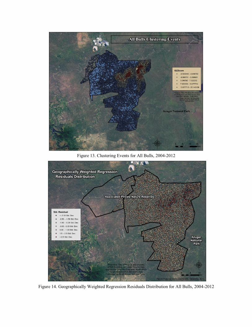
Figure 13. Clustering Events for All Bulls, 2004-2012
Figure 14. Geographically Weighted Regression Residuals Distribution for All Bulls, 2004-2012
Conclusions The completion of this project has allowed for the development of a methodology for assessing
the potential for clustering in the movements of highly mobile, large mammals in an open
savanna ecosystem. The determination that individuals do exhibit this behavior and that their
clustering activity relative to one another is idiosyncratic suggests that there are a host of factors
that determine the relative space utilization of elephants in the Greater Kruger National Park
ecosystem. In the future, analyses of this type could be more illuminating if the ranging activity
of each of these bull elephants could be completed with the knowledge of each bull’s hormonal
state. Bull elephants of this age class cycle hormonally, coming into a rut known as musth,
known to be accompanied by increased rates of travel as bulls seek out receptive females. This
rut is accompanied by surges in testosterone levels that in turn can lead to increased aggression
and could also perhaps explain how bulls arrange themselves on the landscape as they either
avoid conflict or compete with other males for access to females. Additionally, with more time,
being able to rank the relative suitability of each of the represented vegetation types within this
reserve network would perhaps allow us to better understand how to develop a proper predictive
model for understanding where we might be most likely to see clustering events, if in fact the
dominant vegetation community of a certain area has bearing on this variable. Given the nature
of the GPS-location datasets and its inability to meet much of the criteria required for a linear
regression model, more time is needed to develop a predictive model relating environmental
factors to elephant movements in the future.
The potential for spatial analysis to assist in elephant conservation and management in this
ecosystem as well as across the elephant’s range should not be underestimated, as it can provide
managers, scientists, and the general public an understanding of the ways these mega-herbivores
utilize the space that we have left for them. As human populations continue to climb and
elephants are faced with more challenges to sustaining themselves in these protected area
networks, the utilization of GIS will be vital in monitoring the best course that we should take to
ensure that elephants have a place to live, and live safely, for many years to come.
Acknowledgements
We would like to offer profuse thanks to Michelle Henley of Save the Elephants-South Africa
for providing us with the data to complete this class project. Utilizing real-world data has made
learning how to employ GIS a challenging, but rewarding experience.
Additional thanks to our patient instructor and teaching assistants for their help in this learning
process.
Citations
Dean, W. R. J., S. J. Milton, and F. Jeltsch. "Large trees, fertile islands, and birds in arid savanna."
Journal of Arid Environments 41.1 (1999): 61-78.
"Frequently Asked Questions about Elephants." Elephant FAQ. International Union for the
Conservation of Nature, 2011. Web. 07 Dec. 2013.
Izak P.J. Smit, Cornelia C. Grant, Bernard J. Devereux. “Do artificial waterholes influence the way
herbivores use the landscape? Herbivore distribution patterns around rivers and artificial surface
water sources in a large African savanna park.” Biological Conservation, 136.1 (2007): 85-99.
"Kruger National Park." SANParks - Africa's Premier Wildlife Tourism Destinations. South African
National Parks, 2013. Web. 05 Dec. 2013.
Loarie, Scott R., Rudi J. Van Aarde, and Stuart L. Pimm. "Fences and artificial water affect African
savannah elephant movement patterns." Biological conservation 142.12 (2009): 3086-3098.
Mpanduji, Donald G., and Kumrwa A.S Ngomello. “Elephant movements and home range
determinations using GPS/ARGOS satellites and GIS programme: Implication to conservation in
southern Tanzania.” Proceedings from the TAWIRI Annual Scientific Conference (2007).
Stein, Ginny. "Elephant Slaughter Risks Future of Species." Lateline. ABC. Australia, 7 Nov. 2012.
Lateline. Australian Broadcasting Corporation, 7 Nov. 2012. Web. 12 Nov. 2012. Transcript
Appendix
Table 1: Summary of GPS-Collar Locations per Bull in the APNR
Bull Name Date of First
Transmission
Date of Last GPS
Point
Total Number of GPS
Locations
Benjamin 3/14/2005 6/22/2005 166
Brazen 10/20/2005 2/17/2007 2,088
Captain
Hook
4/13/2007 3/21/2011 3,449
Classic 5/24/2004 12/31/2012 28,689
Everest 9/27/2006 7/29/2008 14,425
Gower 10/24/2006 3/13/2013 22,217
Intwanda TBD TBD 15,964
Mac 4/19/2005 7/9/2012 409
Matambu 7/24/2008 12/23/2012 13,090
Mellow 4/13/2007 6/30/2011 4,970
Mean # Of Locations
Standard Deviation
~10,547
~9,887
Table 2: Summary of Top Ten Vegetation Communities in the APNR
Vegetation Community Type
Total
Area (sq.
km)
Proportion
of Total
Area
Acacia nigrescens - Combretum apiculatum mixed woodland 190.2436 13.1505%
Colophospermum mopane dense woodland and shrubveld
(thicket)
171.6129 11.8627%
Combretum apiculatum - Xerophyta retinervis low thicket 153.8712 10.6363%
Phragmites australis river beds 140.4546 9.70886%
Combretum apiculatum - Grewia bicolor low thicket 118.2182 8.17178%
Terminalia sericea - Combretum zeyheri - Pterocarpus
rotundifolius - open woodland
102.2808 7.07011%
Colophospermum mopane - Combretum apiculatum woodland 99.2257 6.85893%
Acacia nigrescens - Terminalia prunioides woodland 92.6144 6.40193%
Combretum apiculatum - Sclerocarya birrea - Strychnos
madagascariensis open woodland
81.6544 5.64432%
Acacia nigrescens - Combretum hereroense open woodland 54.4672 3.76502%

Hot-Spot Analysis Model
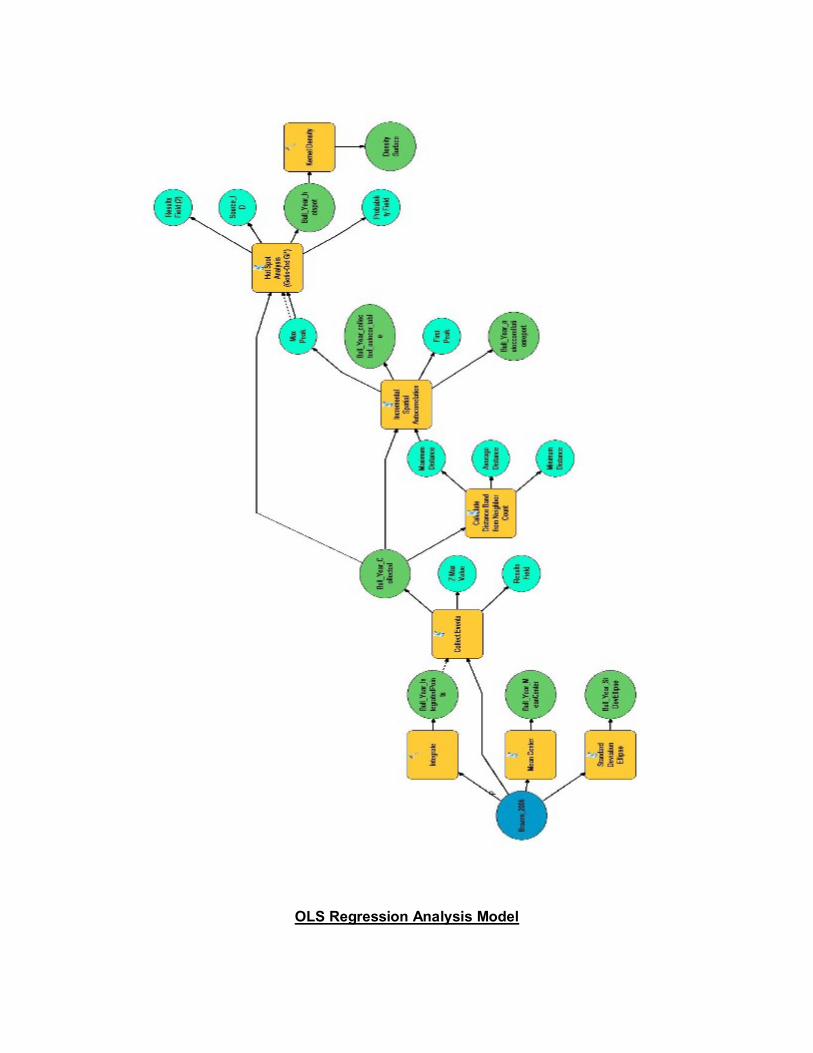
OLS Regression Analysis Model
Recommended