UNIVERSITAT LINZJOHANNES KEPLER JKU
Technisch-NaturwissenschaftlicheFakultat
Linear Diophantine Systems:Partition Analysis and Polyhedral Geometry
DISSERTATION
zur Erlangung des akademischen Grades
Doktor
im Doktoratsstudium der
Technischen Wissenschaften
Eingereicht von:
Zafeirakis Zafeirakopoulos
Angefertigt am:
Research Institute for Symbolic Computation
Beurteilung:
Prof. Peter Paule (Betreuung)Prof. Matthias Beck
Linz, December, 2012

2
This version of the thesis was updated in October 2014. The update only concernsthe presentation and not the content of the thesis.

3
Abstract
The main topic of this thesis is the algorithmic treatment of two problems relatedto linear Diophantine systems. Namely, the first one is counting and the second one islisting the non-negative integer solutions of a linear system of equations/inequalities.
The general problem of solving polynomial Diophantine equations does not admit analgorithmic solution. In this thesis we restrict to linear systems, so that we can treatthem algorithmically. In 1915, MacMahon, in his seminal work “Combinatory Anal-ysis”, introduced a method called partition analysis in order to attack combinatorialproblems subject to linear Diophantine systems. Following that line, in the beginningof this century Andrews, Paule and Riese published fully algorithmic versions of par-tition analysis, powered by symbolic computation. Parallel to that, the last decadessaw significant progress in the geometric theory of lattice-point enumeration, startingwith Ehrhart in the 60’s, leading to important theoretical results concerning generatingfunctions of the lattice points in polytopes and polyhedra. On the algorithmic side ofpolyhedral geometry, Barvinok developed the first polynomial-time algorithm in fixeddimension able to count lattice points in polytopes.
The main goal of the thesis is to connect these two lines of research (partition analysisand polyhedral geometry) and combine tools from both sides in order to construct betteralgorithms.
The first part of the thesis is an overview of conic semigroups from both a geometricand an algebraic viewpoint. This gives a connection between polyhedra, cones andtheir generating functions to generating functions of solutions of linear Diophantinesystems. Next, we provide a geometric interpretation of Elliott Reduction and Omega2(two implementations of partition analysis). The partial-fraction decompositions used inthese two partition-analysis methods are interpreted as decompositions of cones. Withthis insight and employing tools from polyhedral geometry, such as Brion’s theoremand Barvinok’s algorithm, we propose a new algorithm for the evaluation of the Ω≥operator, the central tool in MacMahon’s work on partition analysis. This gives animplementation of partition analysis heavily based on the geometric understanding ofthe method. Finally, a classification of linear Diophantine systems is given, in order tosystematically treat the algorithmic solution of linear Diophantine systems, especiallythe difference between parametric and non-parametric problems.

4
Zusammenfassung
Das Hauptaugenmerk dieser Arbeit liegt auf der algorithmischen Losung zweier Prob-leme, welche im Zusammenhang mit linearen diophantischen Systemen auftreten. Daserste Problem ist die Bestimmung der Anzahl der nicht-negativen, ganzzahligen Losun-gen linearer Systeme von (Un-)Gleichungen, das zweite die Auflistung ebendieser Losun-gen.
Die Losung von polynomiellen diophantischen Gleichungen ist nicht ohne Einschran-kungen algorithmisch handhabbar. Aus diesem Grund beschranken wir uns in der vor-liegenden Arbeit auf lineare Systeme. 1915 fuhrte MacMahon in seinem Werk ”Com-binatory Analysis” eine Methode namens Partition Analysis ein, um kombinatorischeProbleme zu losen, in denen lineare diophantische Systeme auftreten. Darauf aufbauend,jedoch unter weitreichender Miteinbeziehung von Techniken des symbolischen Rechnens,veroffentlichten Andrews, Paule und Riese zu Beginn dieses Jahrhunderts algorithmischeVarianten der Partition Analysis. Parallel dazu gab es in den letzten Jahrzehnten er-hebliche Fortschritte in der geometrischen Theorie zur Aufzahlung von Gittervektoren,beginnend mit Erhart in den 70er Jahren, welche zu wichtigen theoretischen Erkenntnis-sen bezuglich erzeugender Funktionen von Gittervektoren in Polytopen und Polyedernfuhrten. Einen wesentlichen Beitrag in der algorithmischen Entwicklung leistete Barvi-nok mit der Formulierung des ersten Algorithmus, der die Aufzahlung von Gittervektorenin Polytopen ermoglicht und bei fester Dimension eine polynomielle Laufzeit aufweist.
Das Ziel dieser Arbeit is es, beide Forschungsstrange -Partition Analysis und PolyederGeometrie- zu verbinden und die Werkzeuge aus beiden Theorien zu neuen, besserenAlgorithmen zu kombinieren. Der erste Teil gibt einen Uberblick uber konische Halb-gruppen aus zweierlei Blickwinkeln, dem geometrischen und dem algebraischen. Diesermoglicht es uns, die Verbindung von Polyedern, Kegeln und ihrer erzeugenden Funk-tionen zu den erzeugenden Funktionen der Losungen von linearen diophantischen Sys-temen herzustellen. Darauf folgend behandeln wir geometrische Interpretationen vonElliotts Reduction und Omega2, zweier Realisierungen von Partition Analysis. Die Par-tialbruchzerlegungen, welche in diesen beiden Methoden auftreten, werden als Zerlegun-gen von Kegeln interpretiert. Zusammen mit geeigneten Hilfsmitteln aus der PolyederGeometrie, wie etwa dem Satz von Brion und Barvinoks Algorithmus, fuhrt dies zurFormulierung eines neuen Algorithmus zur Anwendung des Omega-Operators, dem zen-tralen Werkzeug in MacMahons Arbeit an Partition Analysis. Wir erhalten darauseine algorithmische Realisierung von Partition Analysis, die entscheidend auf dem ge-ometrischen Verstandnis der Methode basiert. Abschließend wird eine Klassifikationvon linearen diophantischen Systemen eingefuhrt, um systematisch deren algorithmischeLosung aufarbeiten zu konnen. Speziell wird dabei auf die Unterscheidung zwischenparametrischen und nicht-parametrischen Problemen geachtet.

5
Ich erklare an Eides statt, dass ich die vorliegende Dissertation selbststndig und ohnefremde Hilfe verfasst, andere als die angegebenen Quellen und Hilfsmittel nicht benutztbzw. die wortlich oder sinngemaß entnommenen Stellen als solche kenntlich gemachthabe. Die vorliegende Dissertation ist mit dem elektronisch bermittelten Textdokumentidentisch.
Zafeirakis Zafeirakopoulos

6
Acknowledgments
Writing a thesis proved to be harder than what I thought. But, now I know, it wouldhave been impossible without the help of the people who supported me during the last3-4 years.
First I want to thank my advisor Prof. Peter Paule for his support in a range of issuesspanning scientific and everyday life. The two most important things I am grateful to himfor are his suggestion for my PhD topic and his support for my participation in the AIMSQuaRE for “Partition Theory and Polyhedral Geometry”. When I first mentioned tohim my interests, Prof. Paule successfully predicted that the topic of this thesis would befor me exciting enough so that even passing through frustrating and exhausting periods,today I am still as interested as the first day.
Concerning the SQuaRE meetings in the American Institute of Mathematics, I can-not exaggerate about how helpful they were for me. The three weeks of these meetingswere undoubtedly among the most intensive learning and working experiences I ever had.Each one of the participants - Prof. Matthias Beck, Prof. Ben Brown, Prof. MatthiasKoppe and Prof. Carla Savage - helped me in a different way to understand parts of thebeauty lying in the intersection of algebraic combinatorics, polyhedral geometry, numbertheory and the algorithmic methods involved.
Prof. Beck acted as a host during my five months stay in San Francisco visiting SanFrancisco State University in the context of a Marshall Plan Scholarship. Except forbeing excellent in his formal duty as a host (advising me during that period), Matt andTendai acted as real hosts, making my stay in San Francisco a very positive experienceboth in academic and social terms.
During my stay in San Francisco, I met Dr. Felix Breuer with whom I spent agood part of my time there discussing about interesting topics, not always concerningmathematics. During our mathematical discussions emerged a number of topics thathopefully I will have the pleasure to pursue in the future, as well as one chapter of thisthesis. Landing in a city as a stranger always gives a strange feeling, but Felix andChambui contributed in making this feeling negligible.
The first time I landed in a new city was in 2009. The task of making this moveeasier fell on the hands of Veronika, Flavia, Burcin and Ionela. To a large extend, I owethe fact that I am here to them and the great job they did in making Linz a warm place(which is not easy in any sense, especially after living 27 years in Athens), when I firstarrived.
PhD studies is like an extended summer camp. And I don’t just mean exhaustingbut fun. You meet people you like and then they leave, or you leave. You do not knowwhen you will see each other again, possibly next summer in a conference. But, if youare fortunate enough, you make some friends. I was fortunate to meet Max, Hamid,Jakob, Cevo, Nebiye and Madalina, who I do consider as friends.
Distance makes communication between friends harder, but you know that you careabout them and you hope they do the same. Although I love Athens as a city, aftertaking the time to think about what I really miss, it is the people. It is the friends I

7
know for half my life. A couple of them for more than that. For me, the most frustratingthing about living abroad was not being there in the little moments you never care about,except if you are not there.
Giorgos, Dimitris and NN, being themselves in a position similar to mine, distractedme efficiently through these years with pointless but enjoyable discussions. Elias provedto be always a valuable source of information and support. I also want to thank mycolleagues at RISC and especially Manuel, Matteo, Ralf and Veronika for the very usefuldiscussions and directions they gave me on various mathematical topics. At this pointI can say that the bridge at RISC is the place where I made the most friends and alsothe most work done these last years.
Finally, I want to thank my family. My parents supported me in all possible waysduring my studies in Greece and keep supporting me until today. I do owe them morethan I can possibly offer. My brother is still in Athens, in a stay-behind role. I owe tohim my luxury of being able to leave in order to pursue my goals. Achieving one goalonly asks for the next one. And for me that is to be able to support Ilke for the restof my life, the way she supported me during these years. Good that she is an endlesssource of happiness and inspiration for me.

8

Contents
1 Geometry, Algebra and Generating Functions 151.1 Polyhedra, Cones and Semigroups . . . . . . . . . . . . . . . . . . . . . . 151.2 Formal Power Series and Generating Functions . . . . . . . . . . . . . . . 301.3 Formal Series, Rational Functions and Geometry . . . . . . . . . . . . . . 41
2 Linear Diophantine Systems 512.1 Introduction . . . . . . . . . . . . . . . . . . . . . . . . . . . . . . . . . . . 512.2 Classification . . . . . . . . . . . . . . . . . . . . . . . . . . . . . . . . . . 56
3 Partition Analysis 633.1 Partition Analysis Revisited . . . . . . . . . . . . . . . . . . . . . . . . . . 633.2 Algebraic Partition Analysis . . . . . . . . . . . . . . . . . . . . . . . . . . 83
4 Partition Analysis via Polyhedral Geometry 914.1 Eliminating one variable . . . . . . . . . . . . . . . . . . . . . . . . . . . . 924.2 Eliminating multiple variables . . . . . . . . . . . . . . . . . . . . . . . . . 984.3 Improvements based on geometry . . . . . . . . . . . . . . . . . . . . . . . 1014.4 Conclusions . . . . . . . . . . . . . . . . . . . . . . . . . . . . . . . . . . . 110
A Proof of “Geometry of Omega2” 111
9

10 CONTENTS

Introduction
Some History
One of the earliest recorded uses of geometry as a counting tool is the notion of figuratenumbers. Ancient Greeks used pebbles (χαλίκι, where the word calculus comes from),in order to do arithmetic. For example, an arrangement of pebbles would be used tocalculate triangular numbers. In general figurate numbers were popular in ancient times.
Today we mostly care about squares and some special cases (like pentagonal numbersin Euler’s celebrated theorem). Among the mathematicians that were interested infigurate numbers was, of course, Diophantus who wrote a book on polygonal numbers(see [25]). After an interesting turn of events, one of the most prominent methods forthe solution of linear Diophantine systems relies on generalizing figurate numbers.
This generalization bears the name of Eugene Ehrhart who made the first major con-tributions to what is today called Ehrhart theory. The goal is to compute and investigateproperties of functions enumerating the lattice points in polytopes. In dimension 2 andfor the simple regular polygons this coincides with the concept of figurate numbers, butnaturally we are interested in higher-dimensional polytopes and polytopes with morecomplicated geometry.
Diophantus in his masterpiece “Arithmetica” dealt with the solution of equations[25]. But in the time of Diophantus, a couple of things were essentially different than inmodern mathematics:
∙ No notion of zero existed.
∙ Fractions were not treated as numbers (Diophantus was the first to do so).
∙ There was no notation for arithmetic.
”Arithmetica” consisted of 13 books, out of which only six survived and possibly an-other four through Arab translations (found recently), dealing with the solution of 130equations. On one hand his work is important because it is the oldest account we havefor indefinite equations (equations with more than one solutions). More importantlythough, Diophantus introduced a primitive notational system for (what later was called)algebra.
For our purposes, the essential part of his work is his view on what is the solution ofan equation. He considered equations with positive rational coefficients whose solutions
11

12 CONTENTS
are positive rationals. Following this path, we consider a Diophantine problem to haveinteger coefficients and non-negative integer solutions.
In 1463 the German mathematician Regiomontanus, traveling to Italy, he came acrossa copy of Arithmetica. He considered it to be an important work when he reported to afriend of his about it. He intended to do the translation, but he could only find six outof the thirteen books that Diophantus mentioned in his introduction, thus he did notproceed [14].
Although the most famous marginal note to be found in a copy of Arithmeticais by Fermat (his last theorem), there is another one which is very interesting. TheByzantine scholar Chortasmenos notes “Thy soul, Diophantus, be with Satan becauseof the difficulty of your problems” (funny enough next to what came to be known asFermat’s last theorem).
This last comment, combined with the note that Diophantus did not have a gen-eral method (after solving the 100th problem, you still have no clue how to attack the101st) is important for us. Of course, for non-linear Diophantine problems one cannotexpect a general method (Hilbert’s 10th problem). But we present algorithmic solutions(developed during the last century) for linear Diophantine systems and examine theirconnections.
Contributions
The main contribution of this thesis is in the direction of connecting partition analysis, amethod for solving linear Diophantine systems, with polyhedral geometry. The analyticviewpoint of traditional partition analysis methods (due to Elliott, MacMahon, An-drews, Paule and Riese) is interpreted in the context of polyhedral geometry. Throughthis interpretation we are allowed to use tools from geometry in order to enhance thealgorithmic procedures and the understanding of partition analysis. More precisely, themain contributions are:
Geometric and algebraic interpretation of partition analysis
∙ In Theorem 3.2 a geometric interpretation of the generalized partial fraction de-composition employed in Omega2 is given.
∙ We define geometric objects related to the crude generating function and providea geometric version of the Ω≥ operator.
∙ An algebraic version of Ω≥ is given based on gradings of algebraic structures anda variant of Hilbert series.

CONTENTS 13
Algorithmic contributions to partition analysis
∙ A new algorithm for the evaluation of the Ω≥ operator, following the traditionalparadigm of recursive elimination of 𝜆 variables (see Section 4.1).
∙ A new algorithm, motivated by the geometric understanding of the action of Ω≥,that performs simultaneous elimination of all 𝜆 variables (see Section 4.2).
A second goal of the thesis, especially given the interest in algorithmic solutions, isthe classification of linear Diophantine problems. In the literature the notion of a linearDiophantine problem is not consistent and depends on the motivation of the author.
Finally, we note that the main reason why we believe it is important to explore suchconnections, although in both contexts (partition analysis and polyhedral geometry)there are already methods to attack the problem, is that knowledge transfer from onearea to another often helps to develop algorithmic tools that are more efficient.

14 CONTENTS

Chapter 1
Geometry, Algebra andGenerating Functions
In this chapter we present a basic introduction to geometric, algebraic and generatingfunction related concepts that will be used in later chapters. This introduction is notmeant to be complete but rather a recall of basic notions mostly to set up notation. InSection 1.1, some geometric notions and the discrete analog of cones are presented. Fora detailed introduction see [17, 11, 38]. In Section 1.2 a hierarchy of algebraic structuresrelated to formal power series is presented first and then an introduction to generatingfunctions is given. Finally, in Section 1.3 we present the relation of formal power seriesand generating functions via polyhedral geometry and give a short description of moreadvanced geometric tools we will use later.
We note that in this chapter we will use boldface fonts for vectors and the multi-indexnotation x𝑎 = 𝑥𝑎11 𝑥𝑎22 . . . , 𝑥𝑎𝑑𝑑 .
1.1 Polyhedra, Cones and Semigroups
In this section we give a short introduction to polyhedra and polytopes. We define thefundamental objects of polyhedral geometry and provide terminology and notation thatwill be used later. For a more detailed introduction to polyhedral geometry see [17, 38]and references therein.
All of the theory developed in this section takes place in some Euclidean space. Forsimplicity of notation and clarity, we agree this to be R𝑑 for some 𝑑 ∈ N. We fix 𝑑 todenote the dimension of the ambient space R𝑑.
In Section 1.1.1 we will introduce polyhedra and in Section 1.1.2 we discuss aboutpolytopes, while in Section 1.1.3 we will present definitions and notation related topolyhedral cones. In Section 1.1.4 we introduce semigroups and their connection topolyhedral cones.
15
16 CHAPTER 1. GEOMETRY, ALGEBRA AND GENERATING FUNCTIONS
1.1.1 Polyhedra
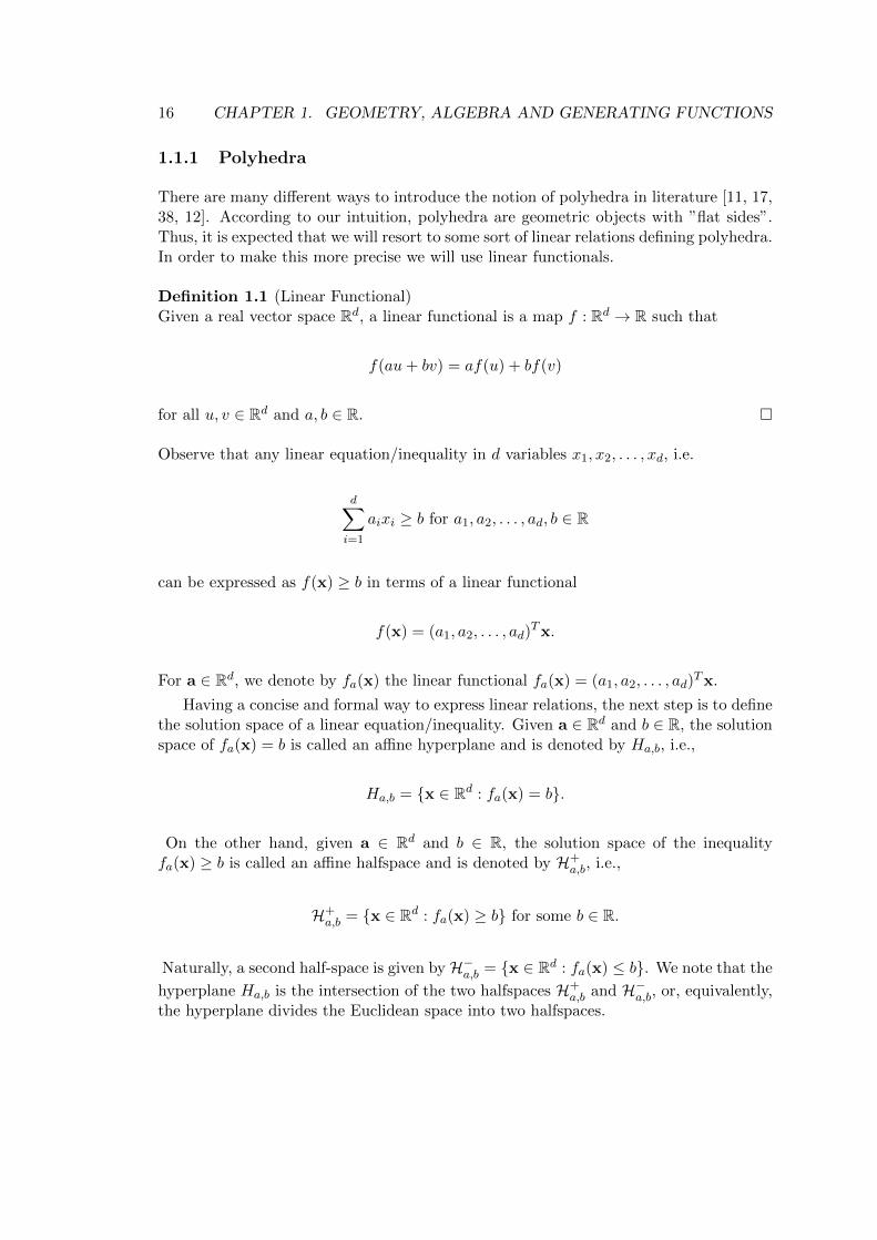
There are many different ways to introduce the notion of polyhedra in literature [11, 17,38, 12]. According to our intuition, polyhedra are geometric objects with ”flat sides”.Thus, it is expected that we will resort to some sort of linear relations defining polyhedra.In order to make this more precise we will use linear functionals.
Definition 1.1 (Linear Functional)Given a real vector space R𝑑, a linear functional is a map 𝑓 : R𝑑 → R such that
𝑓(𝑎𝑢+ 𝑏𝑣) = 𝑎𝑓(𝑢) + 𝑏𝑓(𝑣)
for all 𝑢, 𝑣 ∈ R𝑑 and 𝑎, 𝑏 ∈ R. �
Observe that any linear equation/inequality in 𝑑 variables 𝑥1, 𝑥2, . . . , 𝑥𝑑, i.e.
𝑑∑𝑖=1
𝑎𝑖𝑥𝑖 ≥ 𝑏 for 𝑎1, 𝑎2, . . . , 𝑎𝑑, 𝑏 ∈ R
can be expressed as 𝑓(x) ≥ 𝑏 in terms of a linear functional
𝑓(x) = (𝑎1, 𝑎2, . . . , 𝑎𝑑)𝑇x.
For a ∈ R𝑑, we denote by 𝑓𝑎(x) the linear functional 𝑓𝑎(x) = (𝑎1, 𝑎2, . . . , 𝑎𝑑)𝑇x.
Having a concise and formal way to express linear relations, the next step is to definethe solution space of a linear equation/inequality. Given a ∈ R𝑑 and 𝑏 ∈ R, the solutionspace of 𝑓𝑎(x) = 𝑏 is called an affine hyperplane and is denoted by 𝐻𝑎,𝑏, i.e.,
𝐻𝑎,𝑏 = {x ∈ R𝑑 : 𝑓𝑎(x) = 𝑏}.
On the other hand, given a ∈ R𝑑 and 𝑏 ∈ R, the solution space of the inequality𝑓𝑎(x) ≥ 𝑏 is called an affine halfspace and is denoted by ℋ+
𝑎,𝑏, i.e.,
ℋ+𝑎,𝑏 = {x ∈ R𝑑 : 𝑓𝑎(x) ≥ 𝑏} for some 𝑏 ∈ R.
Naturally, a second half-space is given by ℋ−𝑎,𝑏 = {x ∈ R𝑑 : 𝑓𝑎(x) ≤ 𝑏}. We note that the
hyperplane 𝐻𝑎,𝑏 is the intersection of the two halfspaces ℋ+𝑎,𝑏 and ℋ
−𝑎,𝑏, or, equivalently,
the hyperplane divides the Euclidean space into two halfspaces.
1.1. POLYHEDRA, CONES AND SEMIGROUPS 17
𝑥
𝑦
𝑧
𝑥
𝑦
𝑧
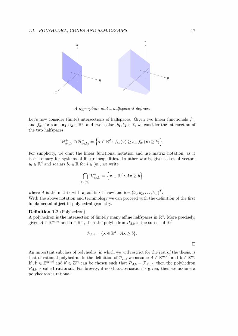
A hyperplane and a halfspace it defines.
Let’s now consider (finite) intersections of halfspaces. Given two linear functionals 𝑓𝑎1and 𝑓𝑎2 for some a1,a2 ∈ R𝑑, and two scalars 𝑏1, 𝑏2 ∈ R, we consider the intersection ofthe two halfspaces
ℋ+𝑎1,𝑏1∩ℋ+
𝑎2,𝑏2={x ∈ R𝑑 : 𝑓𝑎1(x) ≥ 𝑏1, 𝑓𝑎2(x) ≥ 𝑏2
}For simplicity, we omit the linear functional notation and use matrix notation, as itis customary for systems of linear inequalities. In other words, given a set of vectorsai ∈ R𝑑 and scalars 𝑏𝑖 ∈ R for 𝑖 ∈ [𝑚], we write⋂
𝑖∈[𝑚]
ℋ+𝑎𝑖,𝑏𝑖
={x ∈ R𝑑 : 𝐴x ≥ 𝑏
}
where 𝐴 is the matrix with ai as its 𝑖-th row and 𝑏 = (𝑏1, 𝑏2, . . . , 𝑏𝑚)𝑇 .
With the above notation and terminology we can proceed with the definition of the firstfundamental object in polyhedral geometry.
Definition 1.2 (Polyhedron)A polyhedron is the intersection of finitely many affine halfspaces in R𝑑. More precisely,given 𝐴 ∈ R𝑚×𝑑 and b ∈ R𝑚, then the polyhedron 𝒫𝐴,𝑏 is the subset of R𝑑
𝒫𝐴,𝑏 = {x ∈ R𝑑 : 𝐴x ≥ 𝑏}.
�
An important subclass of polyhedra, in which we will restrict for the rest of the thesis, isthat of rational polyhedra. In the definition of 𝒫𝐴,𝑏 we assume 𝐴 ∈ R𝑚×𝑑 and b ∈ R𝑚.If 𝐴′ ∈ Z𝑚×𝑑 and 𝑏′ ∈ Z𝑚 can be chosen such that 𝒫𝐴,𝑏 = 𝒫𝐴′,𝑏′ , then the polyhedron𝒫𝐴,𝑏 is called rational. For brevity, if no characterization is given, then we assume apolyhedron is rational.

18 CHAPTER 1. GEOMETRY, ALGEBRA AND GENERATING FUNCTIONS
𝑥
𝑦
𝑧
A polyhedron
In the beginning of the section we fixed 𝑑 to denote the dimension of the ambientEuclidean space. Moreover, in the definitions of halfspaces and polyhedra we assumedthat these are subsets of R𝑑. Nevertheless, the dimension of a polyhedron is not neces-sarily equal to the dimension of the ambient space as we shall see. In order to define thenotion of the dimension of a polyhedron, we will use the affine hull of a set. Given a realvector space R𝑑 and a set 𝑆 ⊂ R𝑑, then affhullR𝑑 𝑆 is the set of all affine combinationsof elements in 𝑆, i.e.,
affhullR𝑑 𝑆 =
{𝑛∑
𝑖=1
𝛼𝑖si
𝑛 ∈ N*,
𝑛∑𝑖=1
𝛼𝑖 = 1, 𝑎𝑖 ∈ R
}.
Let 𝒫𝐴,𝑏 be a polyhedron in the ambient Euclidean space R𝑑. The dimension of𝒫𝐴,𝑏, denoted by dim𝒫𝐴,𝑏 is defined to be the dimension of the affine hull of 𝒫𝐴,𝑏, i.e.,
dim𝒫𝐴,𝑏 = dimR𝑑 (affhullR𝑑 𝒫𝐴,𝑏) .
Observe that dim𝒫𝐴,𝑏 ≤ 𝑑 in general. If dim𝒫𝐴,𝑏 = 𝑑, then we say that 𝒫𝐴,𝑏 is fulldimensional. A 𝑘-polyhedron is a polyhedron of dimension 𝑘.

1.1. POLYHEDRA, CONES AND SEMIGROUPS 19
𝑥
𝑦
𝑧
A non full-dimensional polyhedron. The ambient space dimension is 3, while thedimension of the polyhedron is 2.
1.1.2 Polytopes
Although we will mostly deal with polyhedra, a very important object, especially whenit comes to lattice-point enumeration, is the polytope. Among the numerous equivalentdefinitions of a polytope, we chose the following:
Definition 1.3 (Polytope)A bounded polyhedron is called a polytope. �
A 3-polytope.
One of the fundamental properties of polytopes, which we will also use in laterchapters, is that a polytope has two equivalent representations, the H-representationand the V-representation. H-representation stands for halfspace representation and itis the set of halfspaces whose intersection is the polytope, i.e., the description we usedin the definition. V-representation stands for vertex representation. A polytope is theconvex hull of its vertices, thus it can be described by a finite set of points in R𝑑. For adetailed proof of this non-trivial fact see Appendix A in [17].

20 CHAPTER 1. GEOMETRY, ALGEBRA AND GENERATING FUNCTIONS
We note that the convex hull of a set of 𝑘 points 𝑆 ∈ R𝑑 is the smallest convex setcontaining 𝑆, or alternatively, the set of all convex combinations of elements from 𝑆, i.e.,
{𝑘∑
𝑖=1
𝛼𝑖si
si ∈ 𝑆,
𝑘∑𝑖=1
𝛼𝑖 = 1, 𝛼 ∈ R
}.
In order to establish terminology and to define the notion of vertex used above, wedefine the notions of supporting hyperplanes and faces of polyhedra and polytopes. Ahyperplane 𝐻 ∈ R𝑑 is said to support a set 𝑆 ⊆ R𝑑 if
∙ 𝑆 is contained in one of the two closed halfspaces determined by 𝐻,
∙ there exists 𝑥 ∈ 𝑆 such that 𝑥 ∈ 𝐻.
In other words, a supporting hyperplane 𝐻 for the polyhedron 𝑃 is a hyperplane thatintersects 𝑃 and leaves 𝑃 entirely on one side.
𝑥𝑦
z
𝑥𝑦
𝑧
Supporting hyperplanes for a cube in 3D
With the use of supporting hyperplanes, we can define now the faces of a polyhedron orpolytope 𝑃 in R𝑑. A face 𝐹 of 𝑃 is the intersection of 𝑃 with a supporting hyperplane𝑆. The dimension of a face 𝐹 is the dimension of affhullR𝑑 𝐹 . A face of dimension𝑘 is called a 𝑘-face. In particular a 0-face is called vertex, a 1-face is called edge orextreme ray and a (dim𝑃 − 1)-face is called facet. We note that a face of a polyhedron(resp. polytope) is again a polyhedron (resp. polytope) and that the definition of facedimension is compatible with the the definition of the dimension of a polyhedron.

1.1. POLYHEDRA, CONES AND SEMIGROUPS 21
A facet, a 1-face and a vertex of a 3-polytope.
Simplices are polytopes of very simple structure and are used as building blocks inpolyhedral geometry. We first define the standard simplex in dimension 𝑑.
Definition 1.4 (Standard Simplex)The standard 𝑑-simplex is the subset of R𝑑 defined by
Δ𝑑 =
{(𝑥1, 𝑥2 . . . , 𝑥𝑑) ∈ R𝑑
𝑑∑𝑖=1
𝑥𝑖 ≤ 1 and 𝑥𝑖 ≥ 0 ∀𝑖
}Equivalently, the standard 𝑑-simplex Δ𝑑 is the convex hull of the 𝑑+ 1 points:
𝑒0 = (0, 0, 0, . . . , 0), 𝑒1 = (1, 0, 0, . . . , 0), 𝑒2 = (0, 1, 0, . . . , 0), . . . 𝑒𝑑 = (0, 0, 0 . . . , 1).
�
In general a 𝑑-simplex is defined to be the convex hull of 𝑑 + 1 affinely independentpoints in R𝑑.
𝑥𝑦
𝑧
𝑥
𝑦
𝑧
The standard 3-simplex and the simplex defined by (1, 1, 0), (2, 3, 0), (0, 3, 0) and(1, 2, 4).

22 CHAPTER 1. GEOMETRY, ALGEBRA AND GENERATING FUNCTIONS
1.1.3 Cones
In polyhedral geometry, the main object is the polyhedron but the main tool is thepolyhedral cone. It is usual to use cones in order to compute with polyhedra andpolytopes or in general to investigate their properties. A fundamental relation is givenby Brion’s theorem (see Theorem 1.3), connecting polyhedra and cones. Cones arepolyhedra of a special type. They are finite intersections of linear halfspaces.
Definition 1.5 (Polyhedral Cone)Given a set of linear functionals 𝑓𝑖(x) : R𝑑 ↦→ R for 𝑖 ∈ [𝑘], we define the polyhedralcone
𝐶 ={x ∈ R𝑑
𝑓𝑖(x) ≥ 0 for all 𝑖 ∈ [𝑘]
}�
For the definition of a cone we used inequalities, complying with the definition of poly-hedron. In what follows though, we will most often define cones via their generators.We first define the conic hull of a set of vectors.
Definition 1.6Given a set of vectors {v1,v2, . . . ,vk} ∈ R𝑑, its conic hull is
co(v1,v2, . . . ,vk) =
{𝑘∑
𝑖=1
𝑟𝑖vi
𝑟𝑖 ∈ R, 𝑟𝑖 ≥ 0
}.
�
The following lemma certifies that a cone can be defined via a finite set of generators.
Lemma 1. A polyhedral cone is the conic hull of its (finitely many) extreme rays. �
Now, given a1,a2, . . . ,ak ∈ R𝑑, we define the cone generated by a1,a2, . . . ,ak as
𝒞R (a1,a2, . . . ,ak) = co (a1,a2, . . . ,ak) =
{x ∈ R𝑑
𝑥 =
𝑘∑𝑖=1
ℓ𝑖ai, ℓ𝑖 ≥ 0, ℓ𝑖 ∈ R
}.
A cone will be called rational if there exists a set of generators for the cone such thatthe generators contain only rational coordinates. As with polyhedra, since all our conesare rational, we omit the characterization.

1.1. POLYHEDRA, CONES AND SEMIGROUPS 23
𝑥
𝑦
𝑧
A polyhedral cone.
Among cones, there are two special types that have a central role in computationalpolyhedral geometry. These are simplicial and unimodular cones. A cone in R𝑑 is calledsimplicial if and only if it is generated by linearly independent vectors in R𝑑. We notethat although usually the definition of a simplicial cone asserts 𝑑 linearly independentgenerators, we do not enforce this restriction. The reason is that often our cones, andpolyhedra in general, will not be full dimensional.
A simplicial cone.
The connection to simplices is more than nominal, in particular a section by a hyperplane(not containing the cone apex) of a simplicial 𝑘-cone is a (𝑘 − 1)-simplex. For the restof the section, except if stated differently, our cones are simplicial.
An object encoding all the information contained in a cone is the fundamentalparallelepiped of the cone.
Definition 1.7 (Fundamental Parallelepiped)Given a simplicial cone 𝐶 = 𝒞R (a1,a2, . . . ,ad) ∈ R𝑑, we define its fundamental paral-lelepiped as
ΠR(𝐶) =
{𝑑∑
𝑖=1
𝑘𝑖ai
𝑘𝑖 ∈ [0, 1)
}

24 CHAPTER 1. GEOMETRY, ALGEBRA AND GENERATING FUNCTIONS
and the set of lattice points in the fundamental parallelepiped as
ΠZ𝑑(𝐶) = ΠR(𝐶) ∩ Z𝑑
�
Note that we assume as working lattice the standard lattice Z𝑑.In the figure below we can see that the cone is spanned by copies of its fundamental
parallelepiped. This is a general fact, i.e., any simplicial cone is spanned by copies of itsfundamental parallelepiped.
(1, 0)
(1, 3)
+(1, 3)
+(1, 0)
The fundamental parallelepiped of the cone generated by (1, 0) and (1, 3).
A cone 𝐶 is called unimodular if and only if ΠZ𝑑(𝐶) = {0}. An equivalent definitionis that the matrix of cone generators is a unimodular matrix, i.e., it has determinantequal to ±1. The following lemma gives a condition for a non full-dimensional cone tobe unimodular.
Lemma 2. Let 𝐶 = 𝒞R (a1,a2, . . . ,an) in R𝑑, for 𝑛 ≤ 𝑑. Let 𝐺 = [a1,a2, . . . ,an],the matrix with ai as columns. If 𝐺 contains a full rank square 𝑛 × 𝑛 submatrix withdeterminant ±1, then 𝐶 is unimodular. �
Proof. Let 𝐼 be an index set such that [𝐺𝑖]𝑖∈𝐼 is a full rank square 𝑛×𝑛 submatrix withdeterminant ±1, where 𝐺𝑖 is the 𝑖-th row of 𝐺. Without loss of generality rearrange thecoordinate system such that 𝐼 are the first 𝑛 coordinates. Let 𝐶𝑛 be the (orthogonal)projection of 𝐶 into 𝑅𝑛. Then 𝐶𝑛 is unimodular. Since projection maps lattice pointsto lattice points, the only way that 𝐶 is not unimodular is that Π(𝐶) contains latticepoints that all project to the origin. In that case, there would be a generator of theform (0, 0, . . . , 0,an+1,an+2, . . . ,am), which contradicts the assumption that [𝐺𝑖]𝑖∈𝐼 isfull rank.
All cones we have seen until now are pointed cones, i.e., they contain a vertex.According to the definition of cone, this is not necessary. A cone may contain a line orhigher dimensional spaces. It is easy to see though, that a cone is pointed if and onlyif it does not contain a line. The unique vertex of a pointed cone is called the apex ofthe cone. Observe that simplicial cones are always pointed.

1.1. POLYHEDRA, CONES AND SEMIGROUPS 25
1.1.4 Semigroups
A semigroup is a very basic algebraic structure, essentially expressing that a set has awell behaved operation. The semigroup operation will be called addition and will bedenoted by +.
Definition 1.8 (Semigroup)A semigroup is a set 𝑆 together with a binary operation + such that
∙ For all 𝑎, 𝑏 ∈ 𝑆 we have 𝑎+ 𝑏 ∈ 𝑆.
∙ For all 𝑎, 𝑏, 𝑐 ∈ 𝑆, we have (𝑎+ 𝑏) + 𝑐 = 𝑎+ (𝑏+ 𝑐).
�
If a semigroup has an identity element, i.e., there exists 𝑒 in 𝑆 such that for all 𝑎 in𝑆 we have 𝑒 + 𝑎 = 𝑎 + 𝑒 = 𝑎, then it is called a monoid. The standard example of amonoid is the set of natural numbers N.
Let 𝑆 be a semigroup with operation +. A set 𝐴 ⊂ 𝑆 is called a subsemigroup of 𝑆if it is closed under the operation +, i.e., for all 𝑎 and 𝑏 in 𝐴 we have that 𝑎+ 𝑏 is in 𝐴.
An important notion connecting the algebraic and geometric points of view is thatof an affine semigroup. We note that all semigroups we consider in what follows areaffine (except if the contrary is explicitly stated) due to Theorem 1.1. For brevity wemay omit the characterization affine later.
Definition 1.9 (Affine semigroup [20])A finitely generated semigroup that is isomorphic to a subsemigroup of Z𝑑 for some 𝑑 iscalled affine semigroup. We will call rank(𝑆) or dimension of 𝑆 the number 𝑑, i.e., theleast dimension such that the semigroup 𝑆 is a subsemigroup of Z𝑑. �
The following theorem by Gordan, in the frame of invariant theory, shows the con-nection between cones and semigroups.
Theorem 1.1 (Gordan’s Lemma, [33])If 𝐶 ⊂ R𝑑 is a rational cone and𝐺 a subgroup of Z𝑑, then 𝐶∩𝐺 is an affine semigroup. �
Gordan’s Lemma allows us to think of lattice points in cones as semigroups. We define,the other way around, the cone of a semigroup.
Definition 1.10 (Cone of 𝑆)Given a subsemigroup 𝑆 of Z𝑑, let 𝒞 (𝑆) be the smallest cone in R𝑑 containing 𝑆. �
Given a semigroup 𝑆, a set {𝑔1, 𝑔2, . . . , 𝑔𝑛} ⊂ 𝑆 is called a generating set for 𝑆 if andonly if for all 𝑎 in 𝑆 there exist ℓ1, ℓ2, . . . , ℓ𝑛 in N such that 𝑎 =
∑𝑛𝑖=0 ℓ𝑖𝑔𝑖. We say that
the semigroup 𝑆 is generated by 𝐺 ⊂ 𝑆 if 𝐺 is a generating set for 𝑆. Note that we donot set any kind of requirements about the elements of the generating set.
We already used the term lattice points in an intuitive way. Formally lattice pointsare elements of a lattice and lattice is a group isomorphic to Z𝑑 (see [20]]). If no otherlattice is specified, then one should assume that lattice means Z𝑑.
We next investigate semigroups that have special structural properties. Let 𝑆 bethe intersection of a rational cone with a subgroup of Z𝑑 (due to Gordan’s Lemma the

26 CHAPTER 1. GEOMETRY, ALGEBRA AND GENERATING FUNCTIONS
intersection is a semigroup). An important question is whether the semigroup generatedby the generators of the cone is equal to 𝑆. In order to formalize the question we needthe notions of integral element and integral closure.
Definition 1.11 (Integral element, [20])Given a lattice ℒ and a subsemigroup 𝑆 of ℒ, an element 𝑥 ∈ ℒ is called integral over 𝑆if 𝑐𝑥 ∈ 𝑆 for some 𝑐 ∈ N. �
Definition 1.12 (Integral Closure)Given a lattice ℒ and a semigroup 𝑆 of ℒ, the set of all elements of ℒ that are integralover 𝑆 is called the integral closure of 𝑆 in ℒ and is denoted by 𝑆𝐿. �
A semigroup 𝑆 is called integrally closed over (or saturated in) a lattice ℒ if 𝑆 = 𝑆ℒ .Thus, the question above becomes “is 𝑆 saturated?”. When we say that 𝑆 is saturated,without specifying the lattice, we mean that it is saturated in Z𝑑. Note that most authorswould mean that the semigroup is saturated in its group of differences Z𝑆, rather thanZ𝑑.
The following proposition provides the connection between a saturated semigroupand its cone.
Proposition 1 (2.1.1. in [20]). Let 𝑆 be an affine semigroup of the lattice ℒ generatedby 𝑔1, 𝑔2, . . . , 𝑔𝑛. Then
∙ 𝑆ℒ = ℒ ∩ 𝒞R (𝑔1, 𝑔2, . . . , 𝑔𝑛)
∙ ∃𝑠1, 𝑠2, . . . , 𝑠𝑘 such that 𝑆ℒ =⋃𝑘
𝑖=1 𝑠𝑖 + 𝑆
∙ 𝑆ℒ is an affine semigroup.
�
Now it is clear that there are three objects we could think of as cones, namely thepolyhedral cone, the lattice points contained in the polyhedral cone and the semigroupgenerated by the generators of the cone. This already shows that we need some notationto distinguish these cases, but before establishing it, we will examine cones whose apicesare not the origin and cones that have open faces.
Let 𝐶 ∈ R𝑑 be the cone 𝒞R (𝑔1, 𝑔2, . . . , 𝑔𝑛) and let 𝐶 ′ ∈ R𝑑 be the cone 𝐶 translatedby the vector 𝑞 ∈ R𝑑. Then we have a bijection 𝜑 : R𝑑 → R𝑑 given by 𝜑(𝑥) = 𝑞 + 𝑥,where addition is the vector space addition, such that 𝐶 ′ = 𝜑(𝐶). As long as 𝑞 is in thelattice ℒ, then lattice points are mapped to lattice points. Although 𝜑 is a semigrouphomomorphism, it is not a monoid homomorphism. This is why we prefer to view themonoids coming from cones with apex at the origin as semigroups and not monoids. It isimportant to note that any unimodular transformation, i.e., a linear transformation givenby a square matrix with determinant ±1, preserves the lattice point structure. 1 Thus
1for translation we have to homogenize in order to have a square matrix with determinant ±1 givingthe transformation. Otherwise we can allow transformations given by a unimodular matrix plus atranslation.
1.1. POLYHEDRA, CONES AND SEMIGROUPS 27
there exists a bijection between the lattice points of the original and the transformedcone. This fact will be used later in order to enumerate lattice points in the fundamentalparallelepiped of a cone.
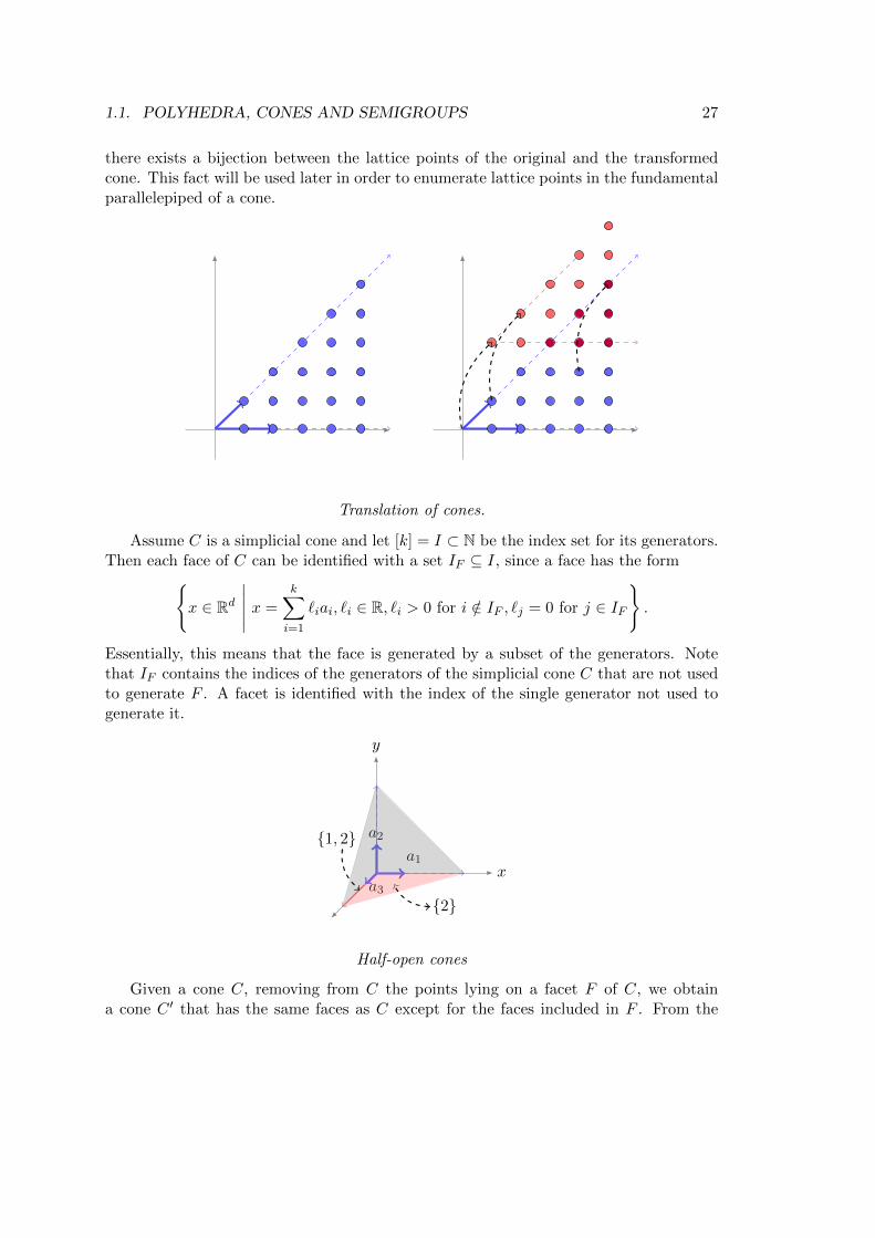
Translation of cones.
Assume 𝐶 is a simplicial cone and let [𝑘] = 𝐼 ⊂ N be the index set for its generators.Then each face of 𝐶 can be identified with a set 𝐼𝐹 ⊆ 𝐼, since a face has the form{
𝑥 ∈ R𝑑
𝑥 =
𝑘∑𝑖=1
ℓ𝑖𝑎𝑖, ℓ𝑖 ∈ R, ℓ𝑖 > 0 for 𝑖 /∈ 𝐼𝐹 , ℓ𝑗 = 0 for 𝑗 ∈ 𝐼𝐹
}.
Essentially, this means that the face is generated by a subset of the generators. Notethat 𝐼𝐹 contains the indices of the generators of the simplicial cone 𝐶 that are not usedto generate 𝐹 . A facet is identified with the index of the single generator not used togenerate it.
𝑥
𝑦
𝑎1
𝑎2
𝑎3{2}
{1, 2}
Half-open cones
Given a cone 𝐶, removing from 𝐶 the points lying on a facet 𝐹 of 𝐶, we obtaina cone 𝐶 ′ that has the same faces as 𝐶 except for the faces included in 𝐹 . From the

28 CHAPTER 1. GEOMETRY, ALGEBRA AND GENERATING FUNCTIONS
previous discussion, for each facet we need only to mention the generator correspondingto that facet. We will use a 0 − 1 vector 𝑜 to express the openess of a cone, i.e., theopeness vector has an entry of 1 in the position 𝑘 if the facet corresponding to the 𝑘-thgenerator is open. If 𝐼 = [𝑘] then the cone is open and if ∅ = 𝐼 ⊂ [𝑘] then the cone ishalf-open.
The above discussion motivates an updated definition of polyhedral cones and relatednotation.
Definition 1.13Given 𝑎1, 𝑎2, . . . , 𝑎𝑘, 𝑞 ∈ Z𝑑 and an index set 𝐼 ⊆ [𝑘], we define:
∙ the (real) cone generated by 𝑎1, 𝑎2, . . . , 𝑎𝑘 at 𝑞 as
𝒞𝐼R (𝑎1, 𝑎2, . . . , 𝑎𝑘; 𝑞) =
{𝑥 ∈ R𝑑 : 𝑥 = 𝑞 +
𝑘∑𝑖=1
ℓ𝑖𝑎𝑖, ℓ𝑖 ≥ 0, ℓ𝑖 ∈ R, ℓ𝑗 > 0 for 𝑗 ∈ 𝐼
}
∙ the semigroup generated by 𝑎1, 𝑎2, . . . , 𝑎𝑘 at 𝑞 as
𝒞𝐼Z (𝑎1, 𝑎2, . . . , 𝑎𝑘; 𝑞) =
{𝑥 ∈ R𝑑 : 𝑥 = 𝑞 +
𝑘∑𝑖=1
ℓ𝑖𝑎𝑖, ℓ𝑖 ≥ 0, ℓ𝑖 ∈ Z, ℓ𝑗 > 0 for 𝑗 ∈ 𝐼
}
∙ given a lattice ℒ, the saturated semigroup generated by 𝑎1, 𝑎2, . . . , 𝑎𝑘 at 𝑞 as
𝒞𝐼R,ℒ (𝑎1, 𝑎2, . . . , 𝑎𝑘; 𝑞) = 𝒞𝐼R (𝑎1, 𝑎2, . . . , 𝑎𝑘; 𝑞) ∩ ℒ
𝒞R ((1, 1), (2, 0)) 𝒞Z ((1, 1), (2, 0)) 𝒞R,Z𝑑 ((1, 1), (2, 0))
𝒞R ((1, 1), (2, 0); (1, 3)) 𝒞Z ((1, 1), (2, 0); (1, 3)) 𝒞R,Z𝑑 ((1, 1), (2, 0); 1, 3))

1.1. POLYHEDRA, CONES AND SEMIGROUPS 29
𝒞{1}R ((1, 1), (2, 0); (1, 3)) 𝒞{1}Z ((1, 1), (2, 0); (1, 3)) 𝒞{1}R,Z𝑑 ((1, 1), (2, 0); (1, 3))
Illustration of the definitions.
�
An important tool in polyhedral geometry is triangulation. A polyhedral objectwith complicated geometry can be decomposed into simpler ones. The building block isthe simplex. Since we are interested mostly in cones, we present the definition for thetriangulation of a cone.
Definition 1.14 (Triangulation of a cone)We define a triangulation of a real cone 𝐶 = 𝒞R (𝑔1, 𝑔2, . . . , 𝑔𝑘) as a finite collection ofsimplicial cones Γ = {𝐶1, 𝐶2, . . . , 𝐶𝑡} such that:
∙⋃𝐶𝑖 = 𝐶,
∙ If 𝐶 ′ ∈ Γ then every face of 𝐶 ′ is in Γ,
∙ 𝐶𝑖 ∩ 𝐶𝑗 is a common face of 𝐶𝑖 and 𝐶𝑗 .
�
The following proposition says that we can triangulate a cone without introducing newrays.
Proposition 2 (see [17]). A pointed convex polyhedral cone 𝐶 admits a triangulation Γwhose 1-dimensional cones are the extreme rays of 𝐶. �
A concept that we will use heavily in later chapters is that of the vertex cone.
Definition 1.15 (Tangent and Feasible Cone)Let 𝑃 ⊆ R𝑑 be a polyhedron and 𝑣 a vertex of 𝑃 , the tangent cone 𝒦𝑣 and the feasiblecone ℱ𝑣 of 𝑃 at 𝑣 are defined by
ℱ𝑣 := {𝑢 | ∃𝛿 > 0 : 𝑣 + 𝛿𝑢 ∈ 𝑃} ,𝒦𝑣 := 𝑣 + ℱ𝑣.
�
We will call 𝒦𝑣 a vertex cone.

30 CHAPTER 1. GEOMETRY, ALGEBRA AND GENERATING FUNCTIONS
1.2 Formal Power Series and Generating Functions
1.2.1 Formal Power Series
Starting from the univariate polynomial ring, we will climb up an hierarchy of algebraicstructures that are related to polyhedral geometry and partition analysis. For a moredetailed exposition see [34, 37] and references therein.
Let K be a field, that we can assume is the field of complex numbers. As usual, wedenote by K[𝑧] the polynomial ring in the variable 𝑧. We will generalize polynomials infour ways, namely by considering fractions of polynomials, allowing an infinite numberof terms, allowing negative exponents and considering more than one variables.
The polynomial ring K[𝑧] contains no zero-divisors, thus it is an integral domain.Since K[𝑧] is an integral domain, we can define its fraction field, i.e., the field of univariaterational functions, denoted by K(𝑧). A polynomial can be considered as a formal sum∑
𝑖∈𝐼𝑎𝑖𝑧
𝑖 for some finite index set 𝐼 ⊆ N and 𝑎𝑖 ∈ K.
If we allow as index sets infinite subsets of the natural numbers, then we obtain formalpowerseries
𝑎(𝑧) =
∞∑𝑖=0
𝑎𝑖𝑧𝑖 for 𝑎𝑖 ∈ K.
Another way to see formal powerseries is as sequences. Given an infinite sequence 𝐴 =[𝑎1, 𝑎2, . . .] with elements from K and a formal variable 𝑧, then 𝑎(𝑧) represents 𝐴. Theusual definition of formal powerseries is as sequences. Define the following two operationsof addition and (Cauchy) multiplication for two formal powerseries 𝑎(𝑧) and 𝑏(𝑧):
𝑎(𝑧) + 𝑏(𝑧) =
∞∑𝑖=0
(𝑎𝑖 + 𝑏𝑖) 𝑧𝑖,
𝑎(𝑧)𝑏(𝑧) =∞∑𝑖=0
⎛⎝ 𝑖∑𝑗=0
𝑎𝑗𝑏𝑖−𝑗
⎞⎠ 𝑧𝑖.
The ring of formal powerseries is the set
KJ𝑧K =
{ ∞∑𝑖=0
𝑎𝑖𝑧𝑖
𝑎𝑖 ∈ K
}
equipped with the above defined addition and multiplication. Note that the ring ofpolynomials is a subring of the ring of formal powerseries. If we allow for polynomialscontaining negative exponents (but only finitely many terms), then we obtain the ring ofLaurent polynomials. We denote this ring by K
[𝑧, 𝑧−1
]or K
[𝑧±1]. Next, we construct
the polynomial ring K[𝑥, 𝑦] as (K[𝑦]) [𝑥], i.e., the ring of polynomials in 𝑥 with coefficientsin the ring K[𝑦] . We define recursively the polynomial ring in 𝑑 variables, denoted by
1.2. FORMAL POWER SERIES AND GENERATING FUNCTIONS 31
K[𝑧1, 𝑧2, . . . , 𝑧𝑑]. The fraction field of K[𝑧1, 𝑧2, . . . , 𝑧𝑑], which is the multivariate versionof the rational function field, is denoted by K(𝑧1, 𝑧2, . . . , 𝑧𝑑). As in the univariate case,allowing for negative exponents, we obtain the multivariate Laurent polynomial ring,denoted by K[𝑧±1
1 , 𝑧±12 , . . . , 𝑧±1
𝑑 ]. Like we did with polynomials, we can construct thering KJ𝑥, 𝑦K of formal powerseries in 𝑥 and 𝑦 as the ring of formal powerseries in 𝑥with coefficients in KJ𝑦K. A ring that we will use extensively in the next chapters isthat of multivariate formal powerseries in 𝑑 variables, defined recursively and denotedby KJ𝑧1, 𝑧2, . . . , 𝑧𝑑K.
An important property of the ring of formal powerseries is given by the following
Lemma 3 (see [27]). If 𝐷 is an integral domain then 𝐷J𝑧K is an integral domain aswell. �
Now, let us define the field of univariate Laurent series, which can be thought ofeither as the fraction field of the ring of univariate formal powerseries or as Laurentpolynomials with finitely many terms of negative exponent but possibly infinitely manyterms of positive exponent. More formally
Definition 1.16 (Univariate formal Laurent series)The set of formal expressions
KL𝑧M =
{∑𝑘∈Z
𝑎𝑘𝑧𝑘
𝑎𝑘 ∈ K, 𝑎𝑘 = 0 for all but finitely many negative values of 𝑘
}
equipped with the usual addition and (Cauchy) multiplication is the field of univariateformal Laurent series. �
The multivariate equivalent is much harder to deal with. In particular, there aremany candidates as appropriate generalizations. We will explore some of them.
In [37], Xin presents two generalizations of formal Laurent series. The first and morestraightforward is that of iterated Laurent series.
Definition 1.17 (Iterated Laurent series, Section 2.1 in [37])The field of iterated Laurent series in 𝑘 variables is defined recursively as
K⟨⟨𝑧1, 𝑧2, . . . , 𝑧𝑘⟩⟩ = K⟨⟨𝑧1, 𝑧2, . . . , 𝑧𝑘−1⟩⟩L𝑧𝑘M
where K⟨⟨𝑧1⟩⟩ = L𝑧1M. �
Next he presents Malcev-Neuman series, which allow the most general setting amongthe ones presented here.
Definition 1.18 (Malcev-Neuman series, Theorem 3-1.6 in [37])Let 𝐺 be a totally ordered monoid and 𝑅 a commutative ring with unit. A formal series𝜂 on 𝐺 has the form
𝜂 =∑𝑔∈𝐺
𝑎𝑔𝑔

32 CHAPTER 1. GEOMETRY, ALGEBRA AND GENERATING FUNCTIONS
where 𝑎𝑔 ∈ 𝑅 and 𝑔 is regarded as a symbol. The support of 𝜂 is defined to be theset {𝑔 ∈ 𝐺 | 𝑎𝑔 = 0}. A Malcev-Neumann series is a formal series on 𝐺 that has a well-ordered support. We define 𝑅𝑤[𝐺] to be the set of all such MN-series. Then 𝑅𝑤[𝐺] is aring. �
In [34], Aparicio-Monforte and Kauers introduce three algebraic structures relatedto multivariate formal Laurent series. They use polyhedral cones and the notion of acompatible additive ordering for their definitions.
Definition 1.19 (Compatible additive ordering [34])Given a pointed simplicial cone 𝐶 ∈ R𝑑 with apex at the origin, a total order ≤ on Z𝑑 iscalled additive if for all 𝑎, 𝑏, 𝑐 ∈ Z𝑑 we have 𝑎 ≤ 𝑏→ 𝑎+𝑐 ≤ 𝑏+𝑐. It is called compatiblewith the cone 𝐶 if 0 ≤ 𝑘 for all 𝑘 ∈ 𝐶. �
First they define the ring of multivariate formal Laurent series supported in a cone.
Definition 1.20 (Multivariate Laurent series from cones [34])Given a pointed cone 𝐶 ∈ R𝑑, the set
K𝐶 J𝑧1, 𝑧2, . . . , 𝑧𝑑K =
{∑𝑘∈𝐶
𝑎𝑘𝑧𝑘
𝑎𝑘 ∈ K
}
equipped with the usual addition and Cauchy multiplication forms a ring . �
A larger ring is obtained if we fix an ordering and consider the collection 𝒞 of all conesthat are compatible with this ordering ≤. Then
K≤ J𝑧1, 𝑧2, . . . , 𝑧𝑑K =⋃𝐶∈𝒞
K𝐶 J𝑧1, 𝑧2, . . . , 𝑧𝑑K
is a ring.
Finally, Aparicio-Monforte and Kauers construct a field of multivariate formal Lau-rent series by taking the union of translates of K≤ J𝑧1, 𝑧2, . . . , 𝑧𝑑K to all lattice points.
K≤L𝑧1, 𝑧2, . . . , 𝑧𝑑M =⋃𝑒∈Z𝑑
𝑧𝑒K≤ J𝑧1, 𝑧2, . . . , 𝑧𝑑K .
The lattice points of a pointed cone form a well-ordered set. Moreover, given theadditive compatible ordering, required by the construction of K≤ J𝑧1, 𝑧2, . . . , 𝑧𝑑K, the sup-port of each object in K≤ J𝑧1, 𝑧2, . . . , 𝑧𝑑K is well-ordered (and 0 is the minimum). Finally,in the construction of K≤L𝑧1, 𝑧2, . . . , 𝑧𝑑M the supports appearing in K≤J𝑧1, 𝑧2, . . . , 𝑧𝑑K maybe translated, but this does not affect the fact that they are well-ordered. This meansthat these three constructions are examples of Malcev-Neuman series, as noted in [34].
Now we will put into the picture of the algebraic structures the sets of power seriesand rational functions occurring in the geometric context. The generating function forthe lattice points of a rational simplicial polyhedral cone is a rational function, see nextsection.
1.2. FORMAL POWER SERIES AND GENERATING FUNCTIONS 33
Definition 1.21 (Polyhedral Laurent Series [16])The space 𝑃𝐿 of polyhedral Laurent series is the K[𝑧±1
1 , 𝑧±12 , . . . , 𝑧±1
𝑑 ]-submodule ofK[[𝑧±1
1 , 𝑧±12 , . . . , 𝑧±1
𝑑 ]] generated by the set of formal series⎧⎪⎨⎪⎩∑
𝑠∈(𝐶∩Z𝑑)
𝑧𝑠
𝐶 is a simplicial rational cone
⎫⎪⎬⎪⎭ .
�
Since any cone can be triangulated by using only simplicial cones, we have that PLcontains the formal power series expressions of the generating functions of all rationalcones. Due to the vertex cone decomposition of polyhedra (see Section 1.3.2), 𝑃𝐿 alsocontains the generating functions of all polyhedra.
The following diagram presents the relations of the structures discussed above.

34 CHAPTER 1. GEOMETRY, ALGEBRA AND GENERATING FUNCTIONS
[𝑧±1 , 𝑧±2 , . . . , 𝑧±𝑛 ]
Malcev-Neuman
K⟨⟨𝑧1, 𝑧2, . . . , 𝑧𝑛⟩⟩ K≥L𝑧1, 𝑧2, . . . , 𝑧𝑛M
K𝐶J𝑧1, 𝑧2, . . . , 𝑧𝑛KK (𝑧1, 𝑧2, . . . , 𝑧𝑛)
KJ𝑧1, 𝑧2, . . . , 𝑧𝑛K
KL𝑧M
K[𝐺]
𝑃𝐿
K[𝑧±11 , 𝑧±1
2 , . . . , 𝑧±1𝑑 ]
Generatingfunctions of
cones
K(𝑧)
K[𝑧1, 𝑧2, . . . , 𝑧𝑛]
KJ𝑧K
K[𝑧±1]
K[𝑧]
Relations of algebraic structures related to polynomials, formal power series andrational functions.

1.2. FORMAL POWER SERIES AND GENERATING FUNCTIONS 35
1.2.2 Generating Functions
One of the most important tools in combinatorics and number theory, when dealingwith infinite sequences, is that of generating functions. The hope is that a generatingfunction, although encoding full information of an infinite object, has a short (or at leastfinite) representation. We will restrict the definitions presented here in a way that coversour use of generating functions without introducing generality that reduces clarity. Fora detailed introduction see [27, 36].
The generating function is a tool for representing infinite sequences in a handy way.A sequence is a map from N to a set of values. We will assume that our values comefrom a field K, but we note that for the most part of the thesis, the only possible valuesare 0 and ±1. The usual notation for a sequence is 𝐴 = [𝑎0, 𝑎1, 𝑎2, . . .] = (𝑎𝑖)𝑖∈N. Wedefine the generating function of 𝐴 as the formal sum
Φ𝐴 =∞∑𝑖=0
𝑎𝑖𝑧𝑖
This is a formal powerseries in KJ𝑧K.If we want to compute the generating function of a set 𝑆, subset of the natural
numbers, we can use the above definition by considering the sequence 𝐴 = [𝑎0, 𝑎1, 𝑎2, . . .],where 𝑎𝑖 = 1 if 𝑖 ∈ 𝑆 and 𝑎𝑖 = 0 otherwise. More formally, we consider the indicatorfunction of the set 𝑆, defined as
[𝑆](𝑥) =
{1 : 𝑥 ∈ 𝑆,0 : 𝑥 /∈ 𝑆.
and then 𝐴 = ([𝑆](𝑖))𝑖∈N. We will use the notation Φ𝑆 for the generating function ofthe set 𝑆, where Φ𝑆 = Φ𝐴 for 𝐴 = ([𝑆](𝑖))𝑖∈N. Naturally, the first example is the naturalnumbers:
ΦN(𝑧) =∑𝑖∈N
[N](𝑖)𝑧𝑖 =∑𝑖∈N
𝑧𝑖 =1
(1− 𝑧).
A slight variation is the sequence of even natural numbers. Then we have
Φ2N(𝑧) =∑𝑖∈N
[2N](𝑖)𝑧𝑖 =∑𝑗∈N
𝑧2𝑗 =1
(1− 𝑧2).
Although these two examples look too simple, it is their multivariate versions that coverthe majority of the cases we are interested in.
With the above definition we can use generating functions to deal with subsets ofthe natural numbers, but this is not sufficient for our purposes. We need to be able todescribe sets containing negative integers. Thus, we extend the definition for subsets ofZ. Given a set 𝑆 ⊆ Z, we define
Φ𝑆 =∑𝑖∈𝑆
𝑧𝑖.

36 CHAPTER 1. GEOMETRY, ALGEBRA AND GENERATING FUNCTIONS
This is not a formal powerseries anymore and depending on the set 𝑆 it may not be aformal Laurent series either.
Although univariate generating functions are very useful for counting, for our pur-poses multivariate ones are essential. The generalization is straightforward.
Definition 1.22 (Generating Function)Given a set 𝑆 ⊂ Z𝑑, we define the generating function of 𝑆 as the formal sum
Φ𝑆 =∑𝑖∈Z𝑑
[𝑆](𝑖)𝑧𝑖.
�
The formal sum representation of a set is no more than syntactic sugar. The represen-tation of a set of numbers or of its formal sum representation have the same (potentially)infinite number of terms. As already stated, the expectation is to have a more condensedrepresentation. A glimpse on that was given in the example of the generating functionof the natural numbers, through the use of the geometric series expansion formula. Weproceed now more formally and setting the necessary notation, defining what a rationalgenerating function is.
Definition 1.23 (Rational Generating Function)Let 𝑆 ⊂ Z𝑑. If there exists a rational function in K(𝑧1, 𝑧2, . . . , 𝑧𝑑), which has a seriesexpansion equal to Φ𝑆 , then we denote that rational function by 𝜌𝑆 (𝑧1, 𝑧2, . . . , 𝑧𝑑) andcall it a rational generating function of 𝑆. �
Here one should note that we make no assumptions on the form of the rationalfunction (e.g. reduced, the denominator has a specific form etc.). This means that aformal powerseries (or formal Laurent series) may have more than one rational functionforms. In the other way, the same rational function can have more than one seriesexpansions. In other words, although the formal sum generating function of a set is a welldefined object, the rational generating function of a set is subject to more parameters.It is not well defined (yet), but extremely useful. We will heavily use rational generatingfunctions and in Section 1.3 we will explain why we are on safe ground.
1.2.3 Generating Functions for Semigroups
In this thesis we deal with generating functions related to polyhedra. For this, it is suffi-cient to compute with generating functions of cones. There are two types of semigroupsthat are of interest for us, the discrete semigroup generated by a set of integer vectorsand the corresponding saturated semigroup. We first compute the generating functionof the semigroup 𝑆 = 𝒞Z ((1, 3), (1, 0)).

1.2. FORMAL POWER SERIES AND GENERATING FUNCTIONS 37
𝒞Z (N) ((1, 3), (1, 0)).The generating function as a formal power series is
Φ𝑆(z) =∑
i∈{𝑘(1,3)+ℓ(1,0)|𝑘,ℓ∈N}
zi =∑𝑘,ℓ∈N
z𝑘(1,3)+ℓ(1,0) =
(∑𝑘∈N
z𝑘(1,3)
)(∑ℓ∈N
zℓ(1,0)
).
Thus, by the geometric series expansion formula we have
𝜌𝑆(z) =
(1
1− z(1,3)
)(1
1− z(1,0)
)=
1(1− 𝑧1𝑧32
)(1− 𝑧1)
.
In general it is easy to see that if a1,a2, . . . ,an are linearly independent, then for thesemigroup 𝑆 = 𝒞Z (a1,a2, . . . ,an) we have
𝜌𝑆(z) =1
(1− za1) (1− za2) · · · (1− zan).
This is true because in the expansion of 1(1−za1 )(1−za2 )···(1−zan ) we get as exponents all
non-negative integer combinations of the exponents in the denominator.Observe that if we translate the semigroup to a lattice point, then the structure does
not change at all.
𝒞Z (N) ((1, 3), (1, 0); (1, 1)).

38 CHAPTER 1. GEOMETRY, ALGEBRA AND GENERATING FUNCTIONS
There is a bijection between 𝒞Z ((1, 3), (1, 0)) and 𝒞Z ((1, 3), (1, 0; (1, 1)), given by 𝑓(s) =s+ (1, 1). Translating this to generating functions we have that
Φ𝒞Z((1,3),(1,0);(1,1))(z) =
∑i∈{𝑘(1,3)+ℓ(1,0)+(1,1)|𝑘,ℓ∈N}
zi
=∑𝑘,ℓ∈N
z𝑘(1,3)+ℓ(1,0)+(1,1)
= z(1,1)
(∑𝑘∈N
z𝑘(1,3)
)(∑ℓ∈N
zℓ(1,0)
).
Now it is clear that the generating function for 𝒞Z ((1, 3), (1, 0; (1, 1)) is rational , namely
𝜌𝒞Z((1,3),(1,0);(1,1))(z) = z(1,1)
(1
1− z(1,3)
)(1
1− z(1,0)
)=
𝑧1𝑧2(1− 𝑧1𝑧32
)(1− 𝑧1)
.
In general for a semigroup 𝑆 = 𝒞Z (a1,a2, . . . ,an;q) we have
𝜌𝑆(z) =zq
(1− za1) (1− za2) · · · (1− zan).
Saturated Semigroup
Let’s consider the saturated semigroup 𝑆 = 𝒞R,Z𝑑 ((1, 3), (1, 0)), and compute its gener-
ating function as a formal powerseries Φ𝑆 =∑𝑠∈𝑆
z𝑠.
𝒞R,Z𝑑 ((1, 3), (1, 0)).
We observe in the following figure that 𝑆 can be partitioned in three sets. The bluepoints are reachable starting from the origin and using only the cone generators. Thered points are reachable by using only the cone generators if we start from the point(1, 1). And similarly for the green ones if we start from (1, 2).

1.2. FORMAL POWER SERIES AND GENERATING FUNCTIONS 39
The saturated semigroup separated in three subsets.
This provides a direct sum decomposition
𝒞R,Z𝑑 ((1, 3), (1, 0)) = 𝒞Z ((1, 3), (1, 0))⊕ 𝒞Z ((1, 3), (1, 0); (1, 1))⊕ 𝒞Z ((1, 3), (1, 0); (1, 2)) .
In general we have the following relation:
𝒞R,Z𝑑 (a1,a2, . . . ,an) = ⊕q∈ΠZ𝑑(𝒞R(a1,a2,...,an))𝒞Z (a1,a2, . . . ,an;q) .
If the apex 𝑞 of the cone of the saturated semigroup is not the origin, we have to translateevery lattice point by 𝑞, thus multiply the generating function by zq.From the relation above and the form of the rational generating function of a discretesemigroup 𝒞Z (a1,a2, . . . ,an;q) we immediately deduce the lemma:
Lemma 4. For a saturated semigroup 𝑆 = 𝒞R,Z𝑑 (a1,a2, . . . ,an; 𝑞) we have
𝜌𝑆(z) =𝑧𝑞∑
𝛼∈ΠZ𝑑(𝒞R(a1,a2,...,an)) z
𝛼
(1− za1) (1− za2) · · · (1− zan).
�
Generating Functions of Open Cones
Given a simplicial cone
𝒞𝐼R (a1,a2, . . . ,ak;q) =
{𝑥 ∈ R𝑑 : 𝑥 = 𝑞 +
𝑘∑𝑖=1
ℓ𝑖a𝑖, ℓ𝑖 ∈ N, ℓ𝑗 > 0 for 𝑗 ∈ 𝐼
}we can apply the inclusion exclusion principle to get an expression of the open cone asa signed sum of closed cones
𝒞𝐼R (a1,a2, . . . ,ak;q) =∑𝑀⊂𝐼
(−1)|𝑀 |𝒞R((ai)𝑖∈𝐼∖𝑀 ;q
).

40 CHAPTER 1. GEOMETRY, ALGEBRA AND GENERATING FUNCTIONS
Example 1. Given the half-open cone 𝒞{1,2}R ((1, 0, 0), (0, 1, 0), (0, 0, 1)) we have
𝒞{1,2}R ((1, 0, 0), (0, 1, 0), (0, 0, 1)) = 𝒞R ((1, 0, 0), (0, 1, 0), (0, 0, 1))
− (𝒞R ((1, 0, 0), (0, 0, 1)) + 𝒞R ((0, 1, 0), (0, 0, 1)))
+ 𝒞R ((0, 0, 1)) .
𝑥
𝑦
𝑎1
𝑎2
𝑎3
{1}
⟨(1, 0, 0), (0, 0, 1)⟩
{2}
{1, 2}
Inclusion-exclusion for 𝒞{1,2}R ((1, 0, 0), (0, 1, 0), (0, 0, 1); 0).
�

1.3. FORMAL SERIES, RATIONAL FUNCTIONS AND GEOMETRY 41
1.3 Formal Series, Rational Functions and Geometry
In this section we review some facts from polyhedral geometry and generating functionsof polyhedra. The main goal is to arrive to a consistent correspondence between ratio-nal generating functions for polyhedra and formal powerseries. This is done throughthe definition of expansion directions. In the end of the section we present two funda-mental theorems from polyhedral geometry for the decomposition of rational generatingfunctions and shortly review Barvinok’s algorithm.
1.3.1 Indicator and rational generating functions
We start by the definition of the space of indicator functions of rational polyhedra.
Definition 1.24 (from [11])The real vector space spanned by indicator functions [𝑃 ] of rational polyhedra 𝑃 ∈ R𝑑
is called the algebra of rational polyhedra in R𝑑 and is denoted by 𝒫Q(R𝑑). �
Theorem 3.3 in [11] is essential for the connection of geometry with rational functions.
Theorem 1.2 (VIII.3.3 in [11])There exists a map
𝜏 : 𝒫Q(R𝑑)→ C (𝑧1, 𝑧2, . . . , 𝑧𝑑)
such that
∙ 𝜏 is a linear transformation (valuation).
∙ If 𝑃 ∈ R𝑑 is a rational polyhedron without lines, then 𝜏 [𝑃 ] = 𝜌𝑃 (z) such that𝜌𝑃∩Z𝑑(z) = Φ
𝑃∩Z𝑑(z), provided that Φ𝑃∩Z𝑑(z) converges absolutely.
∙ For a function 𝑔 ∈ 𝒫Q(R𝑑)and q ∈ Z𝑑, let ℎ(z) = 𝑔(z− q) be a shift of 𝑔. Then
𝜏ℎ = zq𝜏𝑔.
∙ If 𝑃 ∈ R𝑑 is a rational polyhedron containing a line, then 𝜏 [𝑃 ] ≡ 0.
�
Let us see how this map works in an example.
Example 2. Let 𝑑 = 1. We consider the polyhedra:
∙ 𝑃+ = R+ (including the origin)
∙ 𝑃− = R− (including the origin)
∙ 𝑃 = R (the real line)
∙ 𝑃0 = {0}
The associated generating functions (converging in appropriate regions) are:

42 CHAPTER 1. GEOMETRY, ALGEBRA AND GENERATING FUNCTIONS
∙ Φ𝑃+∩Z(𝑧) =∑
𝑚∈𝑃+∩Z𝑧𝑚 =
∞∑𝑚=0
𝑧𝑚 =1
1− 𝑧= 𝜌𝑃+∩Z(𝑧)
∙ Φ𝑃−∩Z(𝑧) =∑
𝑚∈𝑃−∩Z𝑧𝑚 =
0∑𝑚=−∞
𝑧𝑚 =1
1− 𝑧−1= 𝜌𝑃−∩Z(𝑧)
∙ Φ𝑃0∩Z(𝑧) =∑
𝑚∈𝑃0∩Z𝑧𝑚 = 𝑥0 = 1 = 𝜌𝑃0∩Z(𝑧)
From Theorem 1.2 we have that:
∙ 𝜏 [𝑃+] =1
1−𝑧
∙ 𝜏 [𝑃−] =1
1−𝑧−1
∙ 𝜏 [𝑃0] = 1
By inclusion-exclusion we have
[𝑃 ] = [𝑃+] + [𝑃−]− [𝑃0]
Thus one expects that
0 = 𝜏 [𝑃 ] = 𝜏 [𝑃+] + 𝜏 [𝑃−]− 𝜏 [𝑃0] =1
1− 𝑧+
1
1− 𝑧−1− 1
which is indeed the case. In other words
𝜌𝑃∩Z(𝑧) = 𝜌𝑃+∩Z(𝑧) + 𝜌𝑃−∩Z(𝑧)− 𝜌𝑃0∩Z(𝑧).
�
Example 3. Compute the integer points of 𝑃 = [𝑘, 𝑛] ⊂ R for 𝑘 < 𝑛. Let 𝑃1 = [−∞, 𝑛]and 𝑃2 = [𝑘,∞]. Then
[𝑃 ] = [𝑃1] + [𝑃2]− [R]
and
∙ Φ𝑃1∩Z(𝑧) =∑∞
𝑚=𝑘 𝑧𝑚 = 𝑧𝑘
1−𝑧 → 𝜏 [𝑃1] =𝑧𝑘
1−𝑧 = 𝜌𝑃1∩Z(𝑧)
∙ Φ𝑃2∩Z(𝑧) =∑𝑛
𝑚=−∞ 𝑧𝑚 = 𝑧𝑛
1−𝑧−1 → 𝜏 [𝑃2] =𝑧𝑛
1−𝑧−1 = 𝜌𝑃2∩Z(𝑧)
∙ 𝜏 [R] = 0 = 𝜌R∩Z(𝑧)
Thus
𝜌𝑃∩Z =𝑧𝑘
1− 𝑧+
𝑧𝑛
1− 𝑧−1=
𝑧𝑘 − 𝑧𝑛+1
1− 𝑧

1.3. FORMAL SERIES, RATIONAL FUNCTIONS AND GEOMETRY 43
This is expected because𝑧𝑘
1− 𝑧is the generating function of the ray starting at 𝑘, while
𝑧𝑛+1
1− 𝑧is the generating function of the ray starting at 𝑛+1. Subtracting the second from
the first we obtain the segment 𝑃 .If we evaluate 𝜌𝑃∩Z(𝑧) at 𝑧 = 1 (using de l’Hospital’s rule) we get 𝑛 − 𝑘 + 1, the
number of lattice points in 𝑃 . �
Theorem 1.2 provides a correspondence between different representations of gener-ating functions of polyhedra.
Given an indicator function 𝑔 : R𝑑 → {0, 1}, 𝑔 ∈ 𝒫Q(R𝑑), we consider its restriction
𝑔′ : Z𝑑 → {0, 1}. We denote by 𝒫Q(Z𝑑)the set of restricted indicator functions.
𝒫𝑑R 𝒫Q
(R𝑑)
𝒫𝑑Z 𝒫Q
(Z𝑑)
K≥J𝑧K K(𝑧)
𝑓1
𝑓2
𝑓3
𝑓4
𝑓5
𝜏
𝑓6
𝑓7
𝑓8
Figure 1.1: Polyhedra, indicator functions, Laurent and rational generating functions.
The arrows in Figure 1.1 have the following meaning:
𝑓1 Bijection between polyhedra in R𝑑 and their indicator functions.
𝑓2 Map a polyhedron 𝑃 ∈ R𝑑 to 𝑃 ∩ Z𝑑 .
𝑓3 Bijection between sets of lattice points of polyhedra and their Laurent series gen-erating functions.
𝑓4 Bijection between lattice points in polyhedra and their restricted indicator func-tions.
𝑓5 Bijection between restricted indicator function of polyhedra and their Laurentseries generating functions.
𝑓6 Map the restricted indicator function of a polyhedron to a rational function.
𝑓7 Restriction.
𝑓8 Map a Laurent series with support in a polyhedron to a rational function.

44 CHAPTER 1. GEOMETRY, ALGEBRA AND GENERATING FUNCTIONS
In order to be able to map multivariate Laurent series to rational functions we restrictto series in K≥J𝑧K, i.e., we assume that the series have support in a pointed cone [34].The most important maps are 𝑓8 and 𝑓6, but unfortunately they are not bijective. Wewill first see why and then fix this bijection.
When trying to establish the connection between formal powerseries, rational func-tions and polyhedral geometry we encounter problems due to the one-to-many relationbetween rational functions and their Laurent expansions.
Example 4 ([23]). Consider the finite set 𝑆 = {0, 1, 2, . . . , 𝑎} ⊂ N. Its rational gener-ating function is the truncated geometric series
𝜌𝑆(𝑧) =1− 𝑧𝑎+1
1− 𝑧
Now we can rewrite this expression as
𝜌𝑆(𝑧) =1
(1− 𝑧)− 𝑧𝑎+1
(1− 𝑧)
=1
(1− 𝑧)+
𝑧𝑎
(1− 𝑧−1)
and we can expand each summand using the geometric series expansion formula.
𝜌𝑆(𝑧) =1
(1− 𝑧)+
𝑧𝑎
(1− 𝑧−1)
=(𝑧0 + 𝑧1 + 𝑧2 + . . .
)+(𝑧𝑎 + 𝑧𝑎−1 + 𝑧𝑎−2 + . . .
)= 2Φ𝑆(𝑧) +
∞∑𝑖=𝑎+1
𝑧𝑖 +−1∑
𝑖=−∞𝑧𝑖.
If we interpret each of the summands geometrically we end up with the required segmentcounted twice and the rest of the line counted once, which is not what we expected. Thisis due to the fact that the power series expansions around 0 and∞ of the two summands,viewed as analytic functions, have disjoint regions of convergence. In particular we have:
1
(1− 𝑧)=
{𝑧0 + 𝑧1 + 𝑧2 + · · · for|𝑧| < 1,−𝑧−1 − 𝑧−2 − 𝑧−3 · · · for|𝑧| > 1
and
𝑧𝑎
1− 𝑧−1=
{−𝑧𝑎+1 − 𝑧𝑎+2 − 𝑧𝑎+3 · · · for|𝑧| < 1,𝑧𝑎 + 𝑧𝑎−1 + 𝑧𝑎−2 · · · for|𝑧| > 1.
Thus, only the choices where the region of convergence coincide seem natural:

1.3. FORMAL SERIES, RATIONAL FUNCTIONS AND GEOMETRY 45
𝜌𝑆(𝑧) =1
(1− 𝑧)+
𝑧𝑎
(1− 𝑧−1)
=(𝑧0 + 𝑧1 + 𝑧2 + · · ·
)+(−𝑧𝑎+1 − 𝑧𝑎+2 − 𝑧𝑎+3 · · ·
)= Φ𝑆(𝑧)
or
𝜌𝑆(𝑧) =1
(1− 𝑧)+
𝑧𝑎
(1− 𝑧−1)
=(−𝑧−1 − 𝑧−2 − 𝑧−3 · · ·
)+(𝑧𝑎 + 𝑧𝑎−1 + 𝑧𝑎−2 · · ·
)= Φ𝑆(𝑧).
�
Moving from the rational generating function of a set to its geometric representation,we are fixing an expansion direction. This is implicitly done through choosing theLaurent expansion we will interpret geometrically. In Example 4 essentially we pick adirection (either towards positive infinity of negative infinity) and consistently take seriesexpansions with respect to this direction. Even if each of the summands have a perfectlymeaningful expansion with respect to any direction, when we want to make sense out oftheir sum (or simultaneously consider their geometry) we need a consistent choice. Thefollowing example shows how this is important for our purposes.
Example 5. Consider the rational function 𝑓(𝑧) = 𝑧3
(1−𝑧) . One can take either the“forward” or the “backward” expansion of 𝑓 as Laurent power series corresponding toexpansions around 0 or ∞.
𝑧3
(1− 𝑧)=
{𝑧3 + 𝑧4 + 𝑧5 + 𝑧6 + · · · = 𝐹1
−𝑧2 − 𝑧1 − 𝑧0 − 𝑧−1 − · · · = 𝐹2
If we denote by 𝐹 ′𝑖 the power series having only the terms of 𝐹𝑖 that have non-negative
exponents then𝐹 ′1 = 𝑧3 + 𝑧4 + 𝑧5 + 𝑧6 + · · · = Φ[3,∞](𝑧)
and𝐹 ′2 = −𝑧2 − 𝑧1 − 𝑧0 = −Φ[0,2](𝑧)
Observe that the two resulting rational functions 𝜌[3,∞](𝑧) and −𝜌[0,2](𝑧) are different,one is a polynomial and the other is not, although 𝐹1 and 𝐹2 are expansions of the samerational function. �
The operation of keeping only the terms with non-negative exponents is a specialkind of taking intersections in terms of geometry. Moreover, it is an essential part of thecomputation of Ω≥ in a geometric way (see Section 3.1).

46 CHAPTER 1. GEOMETRY, ALGEBRA AND GENERATING FUNCTIONS
Now we will define the notion of forward expansion direction more formally. Forbi ∈ R𝑛, let 𝐵 = {b1,b2, . . . ,bn} be an ordered basis of R𝑛 and
𝐻𝐵 =
{∑𝑖
ℓ𝑖bi : ℓ𝑖 ∈ R, if 𝑗 ∈ [𝑛] is minimal such that ℓ𝑗 = 0 then ℓ𝑗 > 0
}∪ {0}.
We need the notion of the recession cone in order to define directions.
Definition 1.25 (Recession Cone)Given a polyhedron 𝑃 , its recession cone is defined as
rec(𝑃 ) = {𝑦 ∈ R𝑛 : 𝑥+ 𝑡𝑦 ∈ 𝑃 for all 𝑥 ∈ 𝑃 and for all 𝑡 ≥ 0}
�
In order for a Laurent series with support 𝑆 to be well defined we require that thereexists a polyhedron 𝑃 such that 𝑆 ⊂ 𝑃 and rec(𝑃 ) ⊂ 𝐻𝐵, for some ordered basis 𝐵. Wesay that 𝐻𝐵 defines the “forward directions”, in the following sense.
Definition 1.26 (Forward Direction)For any ordered basis 𝐵 of R𝑛 we call 𝑣 ∈ R𝑛 forward if and only if 𝑣 ∈ 𝐻𝐵. �
Note that for every 𝑣 ∈ Z𝑛 − {0} either 𝑣 or −𝑣 is forward. Now we can fix theproblem we had in the diagram about correspondence of generating functions.
Lemma 5. Fix an ordered basis. If Laurent series expansions are taken, consistently,only with respect to forward directions, then there is a bijection between Laurent seriesgenerating functions of lattice points of polyhedra and the respective rational generatingfunctions. �
From now on, we will use series expansions using only forward directions.
Example 6. Let 𝑃1 = [𝑘,∞] and 𝑃2 = [−∞, 𝑛]. We want to compute Φ𝑃1+𝑃2(𝑧) and
𝜌𝑃1+𝑃2(𝑧).
The forward directions are given by the basis 𝐵 = {1} of R and thus 𝐻𝐵 containsall vectors that have positive first coordinate, i.e., 𝑣 ∈ R with 𝑣 > 0. In other words, weaccept any Laurent series that are (possibly) infinite towards ∞, but not towards −∞.
We have
Φ𝑃1∩Z(𝑧) =
∞∑𝑚=𝑘
𝑧𝑚 =𝑧𝑘
1− 𝑧⇒ 𝜏 [𝑃1] =
𝑧𝑘
1− 𝑧= 𝜌𝑃1∩Z(𝑧)
but for the second cone, the expansion should be consistent, i.e., towards ∞. Thus wewill use 𝑃3 = [𝑛+ 1,∞] and the fact that 𝑃2 = R− 𝑃3. We know that [𝑃2] = [R]− [𝑃3]since 𝑃2 ∩ 𝑃3 = ∅. From Theorem 1.2 we know that 𝜏 [R] = 0, thus [𝑃2] = −[𝑃3]. Thisimplies that in the computation of the rational generating function we can ignore R.
Φ𝑃2∩Z(𝑧) = ΦR∩Z(𝑧)− Φ𝑃3∩Z(𝑧) =
∞∑𝑚=−∞
𝑧𝑚 −∞∑
𝑚=𝑛+1
𝑧𝑚

1.3. FORMAL SERIES, RATIONAL FUNCTIONS AND GEOMETRY 47
∼ −∞∑
𝑚=𝑛+1
𝑧𝑚 = − 𝑧𝑛+1
1− 𝑧⇒ 𝜏 [𝑃2] = −
𝑧𝑛+1
1− 𝑧= 𝜌𝑃2∩Z(𝑧).
∼ means that the two Laurent series correspond to polyhedra with the same rationalfunction. Geometrically this means to “flip” the ray from pointing to −∞ to pointing to∞.
Thus
𝜌𝑃∩Z(𝑧) =𝑧𝑘
1− 𝑧− 𝑧𝑛+1
1− 𝑧=
𝑧𝑘 − 𝑧𝑛+1
1− 𝑧.
�
The reason why this phenomenon is not a problem for the classical Ω≥ algorithms (seeSection 3.1) is that by the construction of the crude generating function, we make a choiceof expansion directions for all 𝜆 variables. In particular, when converting the multisumexpression into a rational function, we chose to consider only “forward” expansions forall variables (where forward is defined with respect to the standard basis).
1.3.2 Vertex cone decompositions
We present two theorems that provide formulas for writing the rational generating func-tion of a polyhedron as a sum of rational generating functions of vertex cones. The maindifference between the two formulas is that in the Lawrence-Varchenko formula all conesinvolved are considered as forward expansions, while in Brion’s formula this is not true.
As a matter of fact, Brion’s formula holds true in the indicator functions level modingout lines, which is equivalent to changing the direction of a ray. When reading theformula in the rational function level though, this is not visible since the generatingfunctions of cones obtained by flipping directions are different as Laurent series but thesame as rational functions.
Theorem 1.3 (Brion, 4.5 in [11])Let 𝑃 ⊂ R𝑑 be a rational polyhedron and 𝒦𝑣 be the tangent cone of 𝑃 at vertex 𝑣. Then
[𝑃 ] =∑
𝑣 vertex of 𝑃
[𝒦𝑣] mod polyhedra containing lines
�
Observe that from a general inclusion exclusion formula for indicator functions of tangentcones, if we mod out polyhedra containing lines, then only the vertex cones survive. Asa corollary, applying the map of Theorem1.2, we obtain
Proposition 3 (see [17]). If 𝑃 is a rational polyhedron, then
𝜌𝑃 (z) =∑
𝑣 vertex of 𝑃
𝜌𝒦𝑣(z)
�
48 CHAPTER 1. GEOMETRY, ALGEBRA AND GENERATING FUNCTIONS
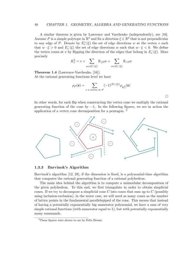
A similar theorem is given by Lawrence and Varchenko (independently), see [16].Assume 𝑃 is a simple polytope in R𝑑 and fix a direction 𝜉 ∈ R𝑑 that is not perpendicularto any edge of 𝑃 . Denote by 𝐸+
𝑣 (𝜉) the set of edge directions 𝑤 at the vertex 𝑣 suchthat 𝑤 · 𝜉 > 0 and 𝐸−
𝑣 (𝜉) the set of edge directions 𝑤 such that 𝑤 · 𝜉 < 0. We definethe vertex cones at 𝑣 by flipping the direction of the edges that belong in 𝐸−
𝑣 (𝜉). Moreprecisely
𝐾𝜉𝑣 = 𝑣 +
∑𝑤∈𝐸+
𝑣 (𝜉)
R≥0𝑤 +∑
𝑤∈𝐸−𝑣 (𝜉)
R<0𝑤
Theorem 1.4 (Lawrence-Varchenko, [16])At the rational generating functions level we have
𝜌𝑃 (z) =∑
𝑣 a vertex in 𝑃
(−1)|𝐸−𝑣 (𝜉)|𝜌
𝐾𝜉𝑣(z)
�
In other words, for each flip when constructing the vertex cone we multiply the rationalgenerating function of the cone by −1. In the following figures, we see in action theapplication of a vertex cone decomposition for a pentagon. 2
-
-
-
-
-
+
1.3.3 Barvinok’s Algorithm
Barvinok’s algorithm [12, 28], if the dimension is fixed, is a polynomial-time algorithmthat computes the rational generating function of a rational polyhedron.
The main idea behind the algorithm is to compute a unimodular decomposition ofthe given polyhedron. To this end, we first triangulate in order to obtain simplicialcones. If we try to decompose a simplicial cone 𝐶 into cones that sum up to 𝐶 (possiblyusing inclusion-exclusion), in the worst case, we will need as many cones as the numberof lattice points in the fundamental parallelepiped of the cone. This means that insteadof having a potentially exponentially big numerator polynomial, we have a sum of verysimple rational functions (with numerator equal to 1), but with potentially exponentiallymany summands.
2These figures were shown to me by Felix Breuer.

1.3. FORMAL SERIES, RATIONAL FUNCTIONS AND GEOMETRY 49
Barvinok proposed the use of signed decompositions. Instead of decomposing thecone 𝐶 into unimodular cones that are contained in 𝐶, one can find a unimodulardecomposition where cones with generators in the exterior of 𝐶 are involved. In thatcase, the generating functions of the unimodular cones involved in the sum will have asign. The advantage of such a signed unimodular decomposition is that it is computablein polynomial time (in fixed dimension), which implies that the number of unimodularcones is not exponential as well.
Algorithm 1 Summary of Barvinok’s algorithm
Require: 𝑃 ⊂ R𝑑 is a rational polyhedron in h-representation
1: Compute the vertices of 𝑃 , denoted by 𝑣𝑖.2: Compute the vertex cones 𝑃𝑣𝑖 .3: If necessary, triangulate 𝑃𝑣𝑖 .4: Compute a signed unimodular decomposition (find a shortest vector).5: Compute the lattice points in the fundamental parallelepiped of each cone.6: return
∑𝑖=1,2...,(number of cones) 𝜖𝑖
1∏𝑑𝑗=1
(1−zb
]ij) , where 𝜖𝑖 is the sign of the 𝑖-th cone
in the signed decomposition and 𝑏𝑖1, 𝑏𝑖2 . . . , 𝑏𝑖𝑑 are the generators of the 𝑖-th cone.

50 CHAPTER 1. GEOMETRY, ALGEBRA AND GENERATING FUNCTIONS

Chapter 2
Linear Diophantine Systems
’Here lies Diophantus,’ the wonderbehold. Through art algebraic, thestone tells how old: ’God gave him hisboyhood one-sixth of his life, Onetwelfth more as youth while whiskersgrew rife; And then yet one-seventhere marriage begun; In five yearsthere came a bouncing new son. Alas,the dear child of master and sageAfter attaining half the measure ofhis father’s life chill fate took him.After consoling his fate by the scienceof numbers for four years, he endedhis life.’
Diophantus tombstone
The main focus of this thesis is on the solution of linear Diophantine systems. Inthis chapter, we introduce some of their properties and provide a classification that isuseful when considering algorithms for solving linear Diophantine systems.
2.1 Introduction
Definition
As the name suggests we have a linear system of equations/inequalities. From linearalgebra, the standard representation of linear systems is in matrix notation. Since werespect Diophantus’ viewpoint, our matrices will always be in Z𝑚×𝑑. In addition, thereis the restriction that the solutions are non-negative integers.
Let M be the set Z × [𝑡1, 𝑡2, . . . , 𝑡𝑘], where [𝑡1, 𝑡2, . . . , 𝑡𝑘] denotes the multiplicativemonoid generated by 𝑡1, 𝑡2, . . . , 𝑡𝑘. In other words, M is the set of monomials in the
51

52 CHAPTER 2. LINEAR DIOPHANTINE SYSTEMS
variables 𝑡𝑖 with integer coefficients. We first give the definition of a linear Diophantinesystem.
Definition 2.1Given 𝐴 ∈ Z𝑚×𝑑, 𝑏 ∈ M𝑚 and ♦ ∈ {≥,=}, the triple (𝐴, 𝑏,♦) is called a linear Dio-phantine system. Note that the relation is considered componentwise (one inequal-ity/equation per row). Let 𝑆 = {𝑥 ∈ N𝑑|𝐴𝑥♦𝑏}. �
We denote the family of solution sets 𝑆 as 𝑆(t) in order to indicate the dependenceon the parameters. Moreover, we will denote by |𝑆(t)| the function on t mapping eachset in the family to its cardinality. We will refer to the family of sets 𝑆(t) as the solutionset of the linear Diophantine system.
Assuming that 𝑏 lives in (Z× [𝑡1, 𝑡2, . . . , 𝑡𝑘])𝑚 is essential for the understanding of a
certain category of problems, but for many interesting problems one can restrict tohaving constant right-hand side, i.e., 𝑏 ∈ Z𝑚. In the latter case, we use 𝑆 and |𝑆|, sincethe family contains only one member.
Characteristics
A linear Diophantine system has two important characteristics. These are related toits geometry and influence greatly the algorithmic treatment. A linear Diophantinesystem defines a polyhedron, whose lattice points are the solutions to the system. If thepolyhedron is bounded, i.e, it is a polytope, then we say that the linear Diophantinesystem is bounded. If the polyhedron is parametric, we say that the linear Diophantinesystem is parametric. We will clarify the notion of parametric with two examples.
The (vector partition function) problem((1 32 1
),
(𝑏1𝑏2
),≥)
is parametric, since the right hand side contains (honest) elements of Z × [𝑏1, 𝑏2]. Thechoice of 𝑏1 and 𝑏2 can change considerably the geometry of the problem. The changein geometry is apparent for 𝑏1 = 4, 𝑏2 = 9 and 𝑏1 = 4, 𝑏2 = 3 in the following figures.
0 2 4 6 8 10
0
2
4
6
8
0 2 4 6 8 10
0
2
4
6
8

2.1. INTRODUCTION 53
On the other hand, the problem (of symmetric 3× 3 magic squares with magic sum 𝑡)⎛⎝⎛⎝ 1 1 1 0 0 00 1 0 1 1 00 0 1 0 1 1
⎞⎠ ,
⎛⎝ 𝑡𝑡𝑡
⎞⎠ ,=
⎞⎠is not a parametric problem, since the (positive integer) parameter 𝑡 does not changethe geometry of the problem (every element of the right hand side is a non-constantunivariate monomial in 𝑡). In other words, we can consider the polytope 𝑃 , defined bythe linear Diophantine system⎛⎝⎛⎝ 1 1 1 0 0 0
0 1 0 1 1 00 0 1 0 1 1
⎞⎠ ,
⎛⎝ 111
⎞⎠ ,=
⎞⎠and the problem is restated as counting (or listing) lattice points in 𝑡𝑃 , i.e., in dilationsof 𝑃 . Thus 𝑡 is a dilation parameter and is not changing the geometry of the problem.
It is important for any further analysis to define properly the size of a linear Dio-phantine problem. There are three input size quantities that are all relevant concerningthe size of a problem:
∙ 𝐵 is the number of bits needed to represent the matrix 𝐴.
∙ 𝑑 is the number of variables.
∙ 𝑚 is the number of relations (equations/inequalities).
In the number of relations we do not count the non-negativity constraints for thevariables. In the number of variables we do not count parameters in parametric problems.These two rules are essential in order to differentiate between problems and to defineproblem equivalence.
Counting vs Listing
Given a linear Diophantine system, one can ask two questions:
∙ How many solutions are there?
∙ What are the solutions?
The first is called the counting problem, while the second is the listing problem.We are interested in solving these two problems in an efficient way. The listing of thesolutions may be exponentially big in comparison to the input size 𝐵 (or even infinite),thus we need a representation of the answer that encodes the solutions in an efficientway. We resort to the use of generating functions for that reason. More precisely, thesolution to the listing problem is a full (or multivariate) generating function, while forthe counting problem is a counting generating function.

54 CHAPTER 2. LINEAR DIOPHANTINE SYSTEMS
In the literature, depending on the motivation of each author, the problem specifi-cation is (sometimes silently) altered. In order to tackle the problem in an algorithmicway, we have to first resolve the specification issue. The formal definitions we use forthe two problems we are interested in are
Definition 2.2 (Listing Linear Diophantine Problem)Given a linear Diophantine system (𝐴, 𝑏,♦) ∈ Z𝑚×𝑑×M𝑚×{=,≥}, denote by 𝑆(t) thesolution set of the linear Diophantine system. Compute the generating function
ℒ𝐴,𝑏,♦(z,q) =∑t∈Z𝑚
⎛⎝ ∑x∈𝑆(t)
zx
⎞⎠qt.
�
Definition 2.3 (Counting Linear Diophantine Problem)Given a linear Diophantine system (𝐴, 𝑏,♦) ∈ Z𝑚×𝑑×M𝑚×{=,≥}, denote by 𝑆(t) thesolution set of the system. Compute the generating function
𝒞𝐴,𝑏,♦(t) =∑t∈Z𝑚
|𝑆(t)|qt.
�
Complexity
The reason why we restrict to linear systems is that algorithmic treatment of the general(polynomial) problem is not feasible. This is the celebrated Hilbert’s 10th problem, whichMatiyasevich [32] solved in the negative direction. In other words, there is no algorithmto decide if a polynomial has integer solutions.
Although the restriction to linear systems makes the problem algorithmically solv-able, it does not make it efficiently solvable. The problem remains NP-hard.
Reduction
The decision problem of linear Diophantine systems (LDS) is
decide if there exists 𝑥 ∈ N𝑑
such that 𝐴𝑥 ≥ 𝑏
In order to show that LDS is NP-hard we reduce from 3-SAT [26]:
given a boolean expression 𝐵(𝑥) =⋀𝑚
𝑖=1𝐶𝑖 in 𝑑-variables,where 𝐶𝑖 is a disjunction of three literalsdecide if there exists 𝑥 ∈ {0, 1}𝑑 such that 𝐵(𝑥) = 1
2.1. INTRODUCTION 55
For each clause 𝑌𝑖 ∨𝑌𝑗 ∨𝑌𝑘, where 𝑌𝑢 is either 𝑦𝑢 or ¬𝑦𝑢, we construct an inequality𝑋𝑖 +𝑋𝑗 +𝑋𝑘 ≥ 1 where 𝑋𝑢 is 𝑥𝑢 or (1− 𝑥𝑢) accordingly.
Let 𝑎𝑖𝑥 ≥ 𝑏𝑖 be the inequality corresponding to the 𝑖-th clause of 𝐵(𝑥). Moreover,
let 𝑄 =
⎡⎢⎢⎢⎣𝑎1𝑎2...𝑎𝑚
⎤⎥⎥⎥⎦ ∈ Z𝑚×𝑑 , 𝑏+ =
⎡⎢⎢⎢⎣𝑏1𝑏2...𝑏𝑚
⎤⎥⎥⎥⎦ ∈ Z𝑚 , 𝑏− =
⎡⎢⎢⎢⎣−1−1...−1
⎤⎥⎥⎥⎦ ∈ Z𝑑 and 𝐼𝑑 be the rank
𝑑 unit matrix.
Then if 𝐴 =
[𝑄−𝐼𝑑
]and 𝑏 =
[𝑏+
𝑏−
]we have
𝑥 ∈ N𝑑 such that 𝐴𝑥 ≥ 𝑏⇔ 𝐵(𝑥) = 1.
We note that this reduction is polynomial.

56 CHAPTER 2. LINEAR DIOPHANTINE SYSTEMS
2.2 Classification
We examine the hierarchy of problems related to linear Diophantine systems from theperspective of the nature of the problem. Although many problems admit the samealgorithmic solution, their nature may be very diverse. Similarly, problems that looksimilar may differ a lot when it comes to their algorithmic solution. There is a twofoldmotivation for this classification. On one hand, it clarifies (by refining) the specificationsof the linear Diophantine problems. On the other hand, it provides useful insight con-cerning the algorithmics, by providing base, degenerate or special cases for the “general”problems.
Moreover, since many problems are equivalent, it is useful to have an overview of thealternatives one has for solving a particular instance of a problem by reformulating it asan instance of another.
Another important aspect is that a problem (and its solution) may change a lotdepending on whether one is interested in the full generating function ℒ (listing problem)or the counting generating function 𝒞 (counting problem).
Each of these two types of problems contains several subproblems, depending on thedomain of the coefficients and the relation involved (equation or inequality).
2.2.1 Classification
For a problem (𝐴, 𝑏,♦), we will use a four letter notation MHRT, where M is the domainof the matrix 𝐴, H is M if the problem is parametric with respect to 𝑏, O if the problem ishomogeneous or the domain of 𝑏 if the problem is inhomogeneous, R is ≥ or = dependingon whether we have inequalities or equations and T is B for bounded or U for unboundedproblems.
In the diagram we see the inclusion relations (if a class A is included in class B, thenan instance from A is also an instance of B).
The following list gives some rules eliminating some of the cases:
1. *𝑂 *𝐵 has {0} as its solution set.
2. N* ≥ * is unbounded.
3. N𝑂 * * is trivially satisfied (N𝑑 is its solution set).
4. NZ ≥ * is trivially satisfied (N𝑑 is its solution set).
5. NZ=* is infeasible.
We note that a problem is assumed to belong to one of the above classes and notany of its subclasses in order to apply the rules. For example, the last rule means thatthe inhomogeneous part has a negative entry, otherwise we would consider the problemin the class of problems with inhomogeneous part in N.
Omitting the cases covered above, we obtain the following diagram:

2.2. CLASSIFICATION 57
Z,M,=, 𝑈 Z,M,≥, 𝑈
N,M,≥, 𝑈
Z,M,=, 𝐵 Z,M,≥, 𝐵
N,M,=, 𝐵
Z,Z,=, 𝑈 Z,Z,≥, 𝑈
Z,Z,=, 𝐵 Z,Z,≥, 𝐵
Z,N,=, 𝑈 Z,N,≥, 𝑈
N,N,≥, 𝑈
Z,N,=, 𝐵
N,N,=, 𝐵
Z, 0,=, 𝑈 Z, 0,≥, 𝑈
We now present examples for some of the cases and provide names and referencesused in literature when available.

58 CHAPTER 2. LINEAR DIOPHANTINE SYSTEMS
N,N,=, 𝐵
Name: Magic Squares
References: [4], Ch.4. Prop 4.6.21 in [35], S6.2 in [17]
Description: 3× 3 symmetric matrices of row and column sum equal to 𝑛
Matrix 𝐴 vector 𝑏 Parameters⎛⎜⎜⎜⎝1 1 1 0 0 0
0 1 0 1 1 0
0 0 1 0 1 1
⎞⎟⎟⎟⎠⎛⎜⎜⎜⎝
1
1
1
⎞⎟⎟⎟⎠ 𝑛
Listing (𝑧0𝑧1𝑧2𝑧3𝑧4𝑧5𝑞3−1)(𝑧1𝑧5𝑞−1)(𝑧0𝑧4𝑞−1)(𝑧2𝑧3𝑞−1)(𝑧0𝑧3𝑧5𝑞−1)(𝑧1𝑧2𝑧4𝑞2−1)
Counting (1+𝑞+𝑞2
(1−𝑞)4(1+𝑞)
Name: Magic Pentagrams
References: S3, page 14 in [5]
Description: Partitions of 𝑛 into parts satisfying relations given by a pentagram withthe parts as vertices and inequalities given by the edges.
Matrix 𝐴 vector 𝑏⎛⎜⎜⎜⎜⎜⎜⎜⎜⎜⎝
1 0 0 1 0 1 0 0 0 1
1 0 1 0 0 0 1 1 0 0
0 1 0 0 1 1 1 0 0 0
0 0 1 0 1 0 0 0 1 1
0 1 0 1 0 0 0 1 1 0
⎞⎟⎟⎟⎟⎟⎟⎟⎟⎟⎠
⎛⎜⎜⎜⎜⎜⎜⎜⎜⎜⎝
2
2
2
2
2
⎞⎟⎟⎟⎟⎟⎟⎟⎟⎟⎠Listing
𝑞𝑧210𝑧23𝑧
37𝑧
34
(−𝑧3𝑧6+𝑧7𝑧10)(−𝑧3𝑧4+𝑧8𝑧10)(𝑧4𝑧27𝑧9𝑧10𝑞−1)(𝑧2𝑧3𝑧4𝑧7𝑧10𝑞−1)·
1(𝑧3𝑧24𝑧5𝑧7𝑞−1)(𝑧3𝑧24𝑧
27𝑧10𝑞−𝑧1)
Counting (𝑞2+3𝑞+1)(𝑞2+13𝑞+1)(𝑞−1)6

2.2. CLASSIFICATION 59
Z,Z,≥, 𝐵
Name: Solid Partitions on a Cube
References: S4.1 in [4]
Description: Partitions of 𝑛 subject to relations given by a cube where the vertices arethe parts and the directed edges indicate the inequalities.
Matrix 𝐴 vector 𝑏⎛⎜⎜⎜⎜⎜⎜⎜⎜⎜⎜⎜⎜⎜⎜⎜⎜⎜⎜⎜⎜⎜⎜⎜⎜⎜⎜⎜⎜⎜⎜⎜⎜⎜⎜⎜⎜⎜⎝
1 −1 0 0 0 0 0 0
1 0 −1 0 0 0 0 0
1 0 0 0 −1 0 0 0
0 1 0 −1 0 0 0 0
0 1 0 0 0 −1 0 0
0 0 1 −1 0 0 0 0
0 0 1 0 0 0 −1 0
0 0 0 1 0 0 0 −1
0 0 0 0 1 −1 0 0
0 0 0 0 1 0 −1 0
0 0 0 0 0 1 0 −1
0 0 0 0 0 0 1 −1
1 1 1 1 1 1 1 1
−1 −1 −1 −1 −1 −1 −1 −1
⎞⎟⎟⎟⎟⎟⎟⎟⎟⎟⎟⎟⎟⎟⎟⎟⎟⎟⎟⎟⎟⎟⎟⎟⎟⎟⎟⎟⎟⎟⎟⎟⎟⎟⎟⎟⎟⎟⎠
⎛⎜⎜⎜⎜⎜⎜⎜⎜⎜⎝
0...
0
1
−1
⎞⎟⎟⎟⎟⎟⎟⎟⎟⎟⎠
Listing 𝑧4𝑧2𝑧1𝑞3
(1−𝑧6𝑞)(𝑧5𝑞−1)(𝑧1𝑞−1)(𝑧1𝑧2𝑞2−1)(𝑧1𝑧2𝑧4𝑞3−1)(𝑧1𝑧2𝑧3𝑧4𝑞4−1)·
1(𝑧1𝑧2𝑧3𝑧4𝑧5𝑧7𝑞6−1)(𝑧1𝑧2𝑧3𝑧4𝑧5𝑧6𝑧7𝑧8𝑞8−1)
Counting (𝑞16+2𝑞14+2𝑞13+3𝑞12+3𝑞11+5𝑞10+4𝑞9+8𝑞8+4𝑞7+5𝑞6+3𝑞5+3𝑞4+2𝑞3+2𝑞2+1)(𝑞−1)8(𝑞+1)4(𝑞2+1)2(𝑞2+𝑞+1)2(𝑞2−𝑞+1)(𝑞4+1)(𝑞4+𝑞3+𝑞2+𝑞+1)
·1
(𝑞6+𝑞5+𝑞4+𝑞3+𝑞2+𝑞+1)

60 CHAPTER 2. LINEAR DIOPHANTINE SYSTEMS
N,M,=, 𝐵
Name: Vector Partition Function
References: Section 4 in [15]
Description: Non-negative integer counts the natural solutions of
𝑥1 + 2𝑥2 + 𝑥3 = 𝑏1
𝑥1 + 𝑥2 + 𝑥4 = 𝑏2
Matrix 𝐴 vector 𝑏 Parameters⎛⎝1 2 1 0
1 1 0 1
⎞⎠ ⎛⎝ 𝑏1
𝑏2
⎞⎠ 𝑏1, 𝑏2
Counting
⎧⎪⎪⎪⎨⎪⎪⎪⎩𝑏214 + 𝑏1 +
7+(−1)𝑏1
8 , 𝑏1 ≤ 𝑏2
𝑏1𝑏2 −𝑏214 −
𝑏222 + 𝑏1+𝑏2
2 + 7+(−1)𝑏1
8 , 𝑏1 > 𝑏2 >𝑏1−32
𝑏222 −
3·𝑏22 + 1 , 𝑏2 ≤ 𝑏1−3
2
Z, 0,≥, 𝐵
Name: Lecture Hall Partitions
References: [18]
Description: Partitions of 𝑛 where 2𝑎 ≤ 𝑏, 3𝑏 ≤ 2𝑐 and 4𝑐 ≤ 3𝑑.
Matrix 𝐴 vector 𝑏⎛⎜⎜⎜⎝2 −1 0 0
0 3 −2 0
0 0 4 −3
⎞⎟⎟⎟⎠⎛⎜⎜⎜⎝
0
0
0
⎞⎟⎟⎟⎠Listing
−𝑧1𝑧32𝑧43𝑧
54𝑞
13
(𝑧2𝑧3𝑧4𝑞3−1)(𝑧1𝑧22𝑧23𝑧
24𝑞
7−1)(𝑧1𝑧22𝑧33𝑧
34𝑞
9−1)(𝑧1𝑧22𝑧33𝑧
44𝑞
10−1)
Counting (𝑞2−𝑞+1)(𝑞4+1)(𝑞−1)4(𝑞2+𝑞+1)(𝑞4+𝑞3+𝑞2+𝑞+1)

2.2. CLASSIFICATION 61
Z,M,≥, 𝐵
Name: Vector Partition Function
References: Section 4 in [15]
Description: Non-negative integer solutions of−𝑥1 − 2𝑥2 ≥ 𝑏1
−𝑥1 − 𝑥2 ≥ 𝑏2
Matrix 𝐴 vector 𝑏 Parameters⎛⎝−1 −2
−1 −1
⎞⎠ ⎛⎝ 𝑏1
𝑏2
⎞⎠ 𝑏1, 𝑏2
Counting
⎧⎪⎪⎪⎨⎪⎪⎪⎩𝑏214 + 𝑏1 +
7+(−1)𝑏1
8 , 𝑏1 ≤ 𝑏2
𝑏1𝑏2 −𝑏214 −
𝑏222 + 𝑏1+𝑏2
2 + 7+(−1)𝑏1
8 , 𝑏1 > 𝑏2 >𝑏1−32
𝑏222 −
3·𝑏22 + 1 , 𝑏2 ≤ 𝑏1−3
2
Z,Z,≥, 𝑈
Matrix 𝐴 vector 𝑏⎛⎝1 −1
1 −2
⎞⎠ ⎛⎝ 3
−2
⎞⎠
0 2 4 6 8 10
0
2
4
6
8
Listing−𝑧21
(𝑧1−1)(−𝑧21+𝑞)(𝑧21𝑧2−1)
Counting 5𝑞(2𝑞+3)(𝑞−1)3

62 CHAPTER 2. LINEAR DIOPHANTINE SYSTEMS
N,M,≥, 𝑈
Name: Vector Partition Function
Matrix 𝐴 vector 𝑏⎛⎝1 3
2 1
⎞⎠ ⎛⎝ 𝑏1
𝑏2
⎞⎠
0 2 4 6 8 10
0
2
4
6
8
0 2 4 6 8 10
0
2
4
6
8
Listing 𝑁(1−𝑧1)(1−𝑧2)(1−𝑞1𝑧1)(1−𝑞22𝑧1)(1−𝑞1𝑞22𝑧1)(1−𝑞31𝑧2)(1−𝑞2𝑧2)(1−𝑞31𝑞2𝑧2)where 𝑁 = 𝑞52𝑧
31𝑧
32𝑞
71 + 𝑞42𝑧
31𝑧
32𝑞
71 − 𝑞42𝑧
31𝑧
22𝑞
71 − 𝑞32𝑧
21𝑧
22𝑞
71 + 𝑞52𝑧
31𝑧
32𝑞
61 + 𝑞42𝑧
31𝑧
32𝑞
61 −
𝑞52𝑧21𝑧
32𝑞
61 − 𝑞42𝑧
21𝑧
32𝑞
61 − 𝑞32𝑧
21𝑧
32𝑞
61 − 𝑞22𝑧
21𝑧
32𝑞
61 − 𝑞42𝑧
31𝑧
22𝑞
61 + 𝑞42𝑧
21𝑧
22𝑞
61 − 𝑞32𝑧
21𝑧
22𝑞
61 +
𝑞22𝑧21𝑧
22𝑞
61 + 𝑞32𝑧1𝑧
22𝑞
61 + 𝑞2𝑧1𝑧
22𝑞
61 + 𝑞52𝑧
31𝑧
32𝑞
51 + 𝑞42𝑧
31𝑧
32𝑞
51 − 𝑞52𝑧
21𝑧
32𝑞
51 − 𝑞42𝑧
21𝑧
32𝑞
51 −
𝑞32𝑧21𝑧
32𝑞
51 − 𝑞22𝑧
21𝑧
32𝑞
51 + 𝑞32𝑧1𝑧
32𝑞
51 + 𝑞22𝑧1𝑧
32𝑞
51 − 𝑞42𝑧
31𝑧
22𝑞
51 + 𝑞42𝑧
21𝑧
22𝑞
51 − 𝑞32𝑧
21𝑧
22𝑞
51 +
𝑞22𝑧21𝑧
22𝑞
51 −𝑞2𝑧
22𝑞
51 +𝑞32𝑧1𝑧
22𝑞
51 −𝑞22𝑧1𝑧
22𝑞
51 +𝑞2𝑧1𝑧
22𝑞
51 −𝑞42𝑧
31𝑧
22𝑞
41 −𝑞52𝑧
21𝑧
22𝑞
41 −𝑞42𝑧
21𝑧
22𝑞
41 −
3𝑞32𝑧21𝑧
22𝑞
41 − 𝑞22𝑧
21𝑧
22𝑞
41 − 𝑞2𝑧
21𝑧
22𝑞
41 − 𝑞2𝑧
22𝑞
41 + 2𝑞32𝑧1𝑧
22𝑞
41 + 𝑞22𝑧1𝑧
22𝑞
41 + 2𝑞2𝑧1𝑧
22𝑞
41 +
𝑞42𝑧21𝑧2𝑞
41 + 2𝑞32𝑧
21𝑧2𝑞
41 + 2𝑞22𝑧
21𝑧2𝑞
41 + 𝑞2𝑧
21𝑧2𝑞
41 − 𝑞22𝑧1𝑧2𝑞
41 − 𝑞2𝑧1𝑧2𝑞
41 − 𝑞42𝑧
31𝑧
22𝑞
31 +
𝑞42𝑧21𝑧
22𝑞
31−𝑞32𝑧
21𝑧
22𝑞
31+𝑞22𝑧
21𝑧
22𝑞
31−𝑞2𝑧
22𝑞
31+2𝑞32𝑧1𝑧
22𝑞
31+𝑞22𝑧1𝑧
22𝑞
31+2𝑞2𝑧1𝑧
22𝑞
31+𝑞32𝑧
21𝑧2𝑞
31+
𝑞22𝑧21𝑧2𝑞
31−𝑞32𝑧1𝑧2𝑞
31−2𝑞22𝑧1𝑧2𝑞
31−2𝑞2𝑧1𝑧2𝑞
31−𝑧1𝑧2𝑞
31−𝑞42𝑧
31𝑧
22𝑞
21+𝑞42𝑧
21𝑧
22𝑞
21−𝑞32𝑧
21𝑧
22𝑞
21+
𝑞22𝑧21𝑧
22𝑞
21 − 𝑞2𝑧
22𝑞
21 + 𝑞32𝑧1𝑧
22𝑞
21 − 𝑞22𝑧1𝑧
22𝑞
21 + 𝑞2𝑧1𝑧
22𝑞
21 + 𝑞32𝑧
21𝑧2𝑞
21 + 𝑞22𝑧
21𝑧2𝑞
21 + 𝑞2𝑧2𝑞
21 −
𝑞32𝑧1𝑧2𝑞21 − 𝑞22𝑧1𝑧2𝑞
21 − 𝑞2𝑧1𝑧2𝑞
21 −𝑧1𝑧2𝑞
21 +𝑧2𝑞
21 − 𝑞32𝑧
21𝑞1 − 𝑞22𝑧
21𝑞1 − 𝑞2𝑧
21𝑞1 − 𝑞32𝑧
21𝑧
22𝑞1 −
𝑞2𝑧22𝑞1 + 𝑞32𝑧1𝑧
22𝑞1 + 𝑞2𝑧1𝑧
22𝑞1 + 𝑞2𝑧1𝑞1 + 𝑞42𝑧
21𝑧2𝑞1 +2𝑞32𝑧
21𝑧2𝑞1 +2𝑞22𝑧
21𝑧2𝑞1 + 𝑞2𝑧
21𝑧2𝑞1 +
𝑞2𝑧2𝑞1 − 𝑞32𝑧1𝑧2𝑞1 − 2𝑞22𝑧1𝑧2𝑞1 − 2𝑞2𝑧1𝑧2𝑞1 − 𝑧1𝑧2𝑞1 + 𝑧2𝑞1 + 𝑞2𝑧1 − 𝑞22𝑧1𝑧2 − 𝑞2𝑧1𝑧2 +1
Chapter 3
Partition Analysis
3.1 Partition Analysis Revisited
Partition analysis is a general methodology for the treatment of linear Diophantinesystems. The methodology is commonly attributed to MacMahon [31], since he wasthe first to apply it in a way similar to the one used today, that is, for the solution ofcombinatorial problems subject to linear Diophantine systems.
MacMahon’s motivation was the proof of his conjectures about plane partitions. Thiswas his declared goal in Combinatory Analysis. The fact that he failed to actually givean answer to the problem was like signing the death certificate of his own child. Incombination with other reasons, including the lack of interest for computational proce-dures in mathematics for most of the 20th century, MacMahon’s method did not becomemainstream among mathematicians.
Except for the theoretical side of the method, there is an algorithmic aspect. Thecomputational and algorithmic nature of the method was evident since the beginning.MacMahon employed an algorithm of Elliott in order to turn his method into an algo-rithm. In [24], Elliott introduced the basics of the methodology and used it to solvelinear homogeneous Diophantine equations. In particular, Elliott’s method is of inter-est because it is algorithmic (in the strict modern sense of the term). Elliott himself,although lacking modern terminology, is arguing on the termination of the procedure.Naturally, given the lack of computers at that time, MacMahon resorted in findingshortcuts (rules) for the most usual cases. This list of rules, included in CombinatoryAnalysis, he expanded as needed for the problem at hand.
It was Andrews who observed the computational potential of MacMahon’s partitionanalysis and waited for the right problem to apply it. In the late 1990’s, the seminal pa-per of Bousquet–Melou and Eriksson [18] on lecture-hall partitions appeared. Andrewssuggested to Paule to explore the capacity of partition analysis combined with sym-bolic computation. This collaboration gave a series of papers, among which [4] and [5]deal with implementations of two fully algorithmic versions of partition analysis, calledOmega, empowered by symbolic computation.
There are different algorithmic (and non-algorithmic) realizations of the general idea.
63

64 CHAPTER 3. PARTITION ANALYSIS
Their relation is illustrated in the following figure. In what follows we will see in chrono-logical order the milestones of partition analysis. Although the goal is to present thehistory, we will allow for a modern view. In particular, we will see some geometric andalgebraic aspects that help understanding partition analysis.
MacMahon
Xin
Ell Ell2
AndrewsPauleRiese
omega
omega2
Elliott
PolyhedralOmega
3.1.1 Elliott
One of the first references relevant to partition analysis is Elliott’s article “On linearhomogeneous Diophantine equation” [24]. The work of Elliott is exciting, if not foranything else, because it addresses mathematicians that lived a century apart. It wasof interest to MacMahon, who based his method on Elliott’s decomposition, but also to21st century mathematicians for explicitly giving an important algorithm. Although, aswe shall see, the algorithm has very bad complexity, it can be considered as an earlyalgorithm for the enumeration of lattice points in cones (among other things).
The problem Elliott considers is to find all non-negative integer solutions to theequation
𝑚∑𝑖=1
𝑎𝑖𝑥𝑖 −𝑚+𝑛∑
𝑖=𝑚+1
𝑏𝑖𝑥𝑖 = 0 for 𝑎𝑖, 𝑏𝑖 ∈ N. (3.1)
In other words, we consider one homogeneous linear Diophantine equation. It should benoted that Elliott himself (as well as subsequent authors) expressed the equation in theform Diophantus would prefer, without using negative coefficients.
The starting point for Elliott’s work is the fact that even if one computes the set of“simple solutions”, i.e., solutions that are not combinations of others, there are syzygies

3.1. PARTITION ANALYSIS REVISITED 65
preventing us from writing down formulas giving each and every solution of the equationexactly once. He proceeds by explaining that his method computes a generating functionwhose terms are in one-to-one correspondence with the solutions of the equation. Elliottstates that this generating function is obtained “by a finite succession of simple stages”.This sentence exhibits an impressive insight on what an algorithm is, as well as Elliott’srealization that he has an algorithm at hand. We quote Elliott outlining his idea in [24]:
The principle is that in the infinite expansion which is the formal product ofthe infinite expansions1 + 𝜉1𝑢
𝑎1 + 𝜉21𝑢2𝑎1 + · · ·
1 + 𝜉2𝑢𝑎2 + 𝜉22𝑢
2𝑎2 + · · ·...1 + 𝜉𝑚𝑢𝑎𝑚 + 𝜉2𝑚𝑢2𝑎𝑚 + · · ·1 + 𝜉𝑚+1𝑢
−𝑏𝑚+1 + 𝜉2𝑚+1𝑢−2𝑏𝑚+1 + · · ·
1 + 𝜉𝑚+2𝑢−𝑏𝑚+2 + 𝜉2𝑚+2𝑢
−2𝑏𝑚+2 + · · ·...1 + 𝜉𝑚+𝑛𝑢
−𝑏𝑚+𝑛 + 𝜉2𝑚+𝑛𝑢−2𝑏𝑚+𝑛 + · · ·
the terms free from 𝑢 are of the form 𝜉𝑥11 𝜉𝑥2
2 · · · 𝜉𝑥𝑚𝑚 𝜉
𝑥𝑚+1
𝑚+1 𝜉𝑥𝑚+2
𝑚+2 · · · 𝜉𝑥𝑚+𝑛𝑚+𝑛 with
1 for numerical coefficient, where 𝑥1, 𝑥2, . . . , 𝑥𝑚, 𝑥𝑚+1, . . . , 𝑥𝑚+𝑛 are a set ofpositive integers (zero included), which satisfy our Diophantine equation 3.1,and that there is just one such term for each set of solutions.
In other words, the generating function for determining the sets of solu-tions, each once, of 3.1, as sets of exponents of the 𝜉𝑖’s in its several terms,is the expression for the part which is free from 𝑢 of the expansion of
1
(1− 𝜉1𝑢𝑎1) · · · (1− 𝜉𝑚𝑢𝑎𝑚)(1− 𝜉𝑚+1𝑢−𝑏𝑚+1) · · · (1− 𝜉𝑚+𝑛𝑢−𝑏𝑚+𝑛)(3.2)
in the positive powers of the 𝜉𝑖’s.The problem is, in any case, to extract from 3.2, and to examine, this
generating function. The extraction may be effected by a finite number ofeasy steps as follows.
The principle presented here by Elliott is the basis of partition analysis, i.e., intro-ducing an extra variable, denoted by 𝑢 in Elliott and by 𝜆 in modern partition analysis.We switch from 𝜉 and 𝑢 to 𝑧 and 𝜆 in order to conform with more modern notationalconventions. The method of Elliott computes a partial fraction decomposition of anexpression
𝑘∏𝑖
1
1−𝑚𝑖, (3.3)
where 𝑚𝑖 ∈[𝑧1, 𝑧2, . . . , 𝑧𝑘, 𝜆, 𝜆
−1]and 𝑘 ∈ N, into a sum of the form∑ ±1∏(1− 𝑝𝑖)
+∑ ±1∏
(1− 𝑞𝑗)(3.4)

66 CHAPTER 3. PARTITION ANALYSIS
with 𝑝𝑖 ∈ [𝑧1, 𝑧2, . . . , 𝑧𝑘, 𝜆] and 𝑞𝑗 ∈ [𝑧1, 𝑧2, . . . , 𝑧𝑘, 𝜆−1].
We note that some authors refer to rational functions of the form 3.3 as Elliott rationalfunctions. The algorithm is based on the fact
1
(1− 𝑥𝜆𝛼)(1− 𝑦𝜆𝛽 )
=1
1− 𝑥𝑦𝜆𝛼−𝛽
(1
1− 𝑥𝜆𝛼+
1
1− 𝑦𝜆𝛽
− 1
)(3.5)
=1
(1− 𝑥𝑦𝜆𝛼−𝛽)(1− 𝑥𝜆𝛼)+
1
(1− 𝑥𝑦𝜆𝛼−𝛽)(1− 𝑦𝜆𝛽 )− 1
(1− 𝑥𝑦𝜆𝛼−𝛽).
Observe that given 𝛼 and 𝛽 positive integers, after applying 3.5, we obtain a sum ofterms where in each of them either the number of factors containing 𝜆 reduced or theexponent of 𝜆 reduced (in absolute value) in one of the factors while it did not changein the other. This observation is the proof of termination Elliott gives for his algorithm.
Let’s see a very simple example, where by applying (3.5) once, we obtain the desiredpartial fraction decomposition.
Example 7.
1
(1− 𝑥𝜆)(1− 𝑦𝜆)
=1
(1− 𝑥𝑦)(1− 𝑥𝜆)+
1
(1− 𝑥𝑦)(1− 𝑦𝜆)− 1
(1− 𝑥𝑦)
=
(1
(1− 𝑥𝑦)(1− 𝑥𝜆)− 1
(1− 𝑥𝑦)
)+
1
(1− 𝑥𝑦)(1− 𝑦𝜆)
.
Notice that the terms in the parenthesis contain only non-negative 𝜆 exponents, whilethe last term contains only non-positive ones as requested by (3.4). �
Each of the summands in∑𝑖
±1∏𝑗(1− 𝑝𝑖)
can be expanded using the geometric-series
expansion formula. It is easy to see that the summands contributing to the generatingfunction for the solution of Equation 3.1 are exactly the ones where in their expansion
𝜆 does not appear. This happens only for the terms±1∏
𝑘(1− 𝑝𝑘)where all 𝑝𝑘 are 𝜆-free.
Summing up only these terms we get the desired generating function.In order to translate this rational function identity to an identity about cones we
first observe that1
(1− 𝑥𝜆𝛼)(1− 𝑦𝜆𝛽 )
is the generating function of the 2-dimensional cone 𝐶 = 𝒞R ((1, 0, 𝛼), (1, 0,−𝛽)), sinceLemma 2 guarantees that the numerator in the rational generating function of 𝐶 isindeed 1.
Observe that the point (1, 1, 𝛼− 𝛽) is in the interior of the cone 𝐶. This means thatthe cones 𝐴 = 𝒞R ((1, 0, 𝛼), (1, 1, 𝛼− 𝛽)) and 𝐵 = 𝒞R ((1, 0,−𝛽), (1, 1, 𝛼− 𝛽)) subdividethe cone 𝐶. Their intersection is exactly the ray starting from the origin and passing

3.1. PARTITION ANALYSIS REVISITED 67
through (1, 1, 𝛼 − 𝛽). By a simple inclusion-exclusion argument we have the signeddecomposition 𝐶 = 𝐴+ 𝐵 − (𝐴 ∩ 𝐵). This decomposition translated to the generatingfunction level is exactly the partial fraction decomposition employed by Elliott. In theexample shown below, after three applications of Elliott’s decomposition we obtain thedesired cone.
𝑥 𝑦
𝜆
𝑥 𝑦
𝜆
𝑥 𝑦
𝜆
𝑥 𝑦
𝜆
𝑥 𝑦
𝜆
𝑥 𝑦
𝜆
𝑥 𝑦
𝜆
𝑥 𝑦
𝜆
Elliott’s decomposition
The Algorithm
It is easy to see that, after a finite number of steps, we end up with a sum of cones ofthree types:
1. the generators contain only zero last coordinate (𝜆-coordinate);
2. the generators contain only non-negative (but not all zero) last coordinate;
3. the generators contain only non-positive (but not all zero) last coordinate.
Note that all the cones involved are unimodular.For equations we sum up the generating functions corresponding to cones of the 1st
type. For inequalities, we intersect each cone with the non-negative 𝜆 halfspace. Thismeans that we discard the cones of the 3rd type and sum up the generating functions ofthe rest of the cones. Then we (orthogonally) project with respect to the 𝜆-coordinate.The sum of rational generating functions for the lattice points in each cone we obtainedis the partial fraction decomposition obtained by Elliott’s algorithm.

68 CHAPTER 3. PARTITION ANALYSIS
Elliott for Systems
It is important to note that Elliott’s method relies on the fact that the numerators inall the expressions involved are equal to 1. Of course after bringing all the terms thealgorithm returns over a common denominator, there is no guarantee that the numeratorwill be 1. But for each term returned the condition is preserved. Thus it is possible toiteratively apply the algorithm to eliminate 𝜆’s in order to solve systems of equationsor inequalities. We note that Elliott proves that the numerators will always be ±1. Norepetitions occur in the computed expression.
Example 8. The system of linear homogeneous inequalities {7𝑎 − 𝑏 ≥ 0, 𝑎 − 3𝑏 ≥ 0}can be solved by Elliott, resulting in 1
(1−𝑥)(1−𝑥3𝑦), if the inequality 𝑎 − 3𝑏 ≥ 0 is treated
first. If the order is reversed then the intermediate expression
−1− 𝑥𝑦6
𝜆17 − 𝑥𝑦5
𝜆14 − 𝑥𝑦4
𝜆11 − 𝑥𝑦3
𝜆8 − 𝑥𝑦2
𝜆5 − 𝑥𝑦𝜆2
(1− 𝑥𝜆)(1− 𝑥𝑦7
𝜆20 )
is violating the condition that numerators are equal to 1.The first inequality of the system is redundant, i.e., if we ignore it the solution set does
not change. Thus, choosing the right order, the intermediate expression 1(1−𝑥𝜆7)(1−𝑥3𝑦𝜆20)
behaves well. We could still apply Elliott’s method if we did not bring the intermediateexpression over a common denominator. �
3.1.2 MacMahon
MacMahon presented his investigations concerning integer partition theory in a series ofseven memoirs, published between 1895 and 1916. In the second memoir [30], MacMahonobserves that the theory of partitions of numbers develops in parallel to that of linearDiophantine equations and in his masterpiece “Combinatory Analysis” [31] he notes:
The most important part of the volume. Sections VIII et seq., arises frombasing the theory of partitions upon the theory of Diophantine inequalities.This method is more fundamental than that of Euler, and leads directly to ahigh degree of generalization of the theory of partitions, and to several inves-tigations which are grouped together under the title of “Partition Analysis”.
In order to attack the problem of solving linear Diophantine systems, MacMahon(like Elliott) introduced extra variables. Let 𝐴 ∈ Z𝑚×𝑑 and b ∈ Z𝑚. We want to findall x ∈ N𝑑 satisfying 𝐴x ≥ b. The generating function of the solution set is
Φ𝐴,𝑏(z) =∑𝐴x≥b
zx.
Let’s introduce extra variables 𝜆1, 𝜆2, . . . , 𝜆𝑚 to encode the inequalities 𝐴x ≥ b, trans-forming the generating function to ∑
x∈N𝑑,𝐴x≥b
𝜆𝐴xzx

3.1. PARTITION ANALYSIS REVISITED 69
The 𝜆 variables are introduced to encode the inequalities, but the solutions we aresearching for live in dimension 𝑑. The 𝜆 dimensions are used to control that aftera certain decomposition we can filter out the solutions involving negative exponents.Following this principle, MacMahon introduced the concept of the crude generatingfunction. But before that, we need to see the Ω≥ operator. MacMahon defined it inArticle 66 of [30]:
Suppose we have a function
𝐹 (𝑥, 𝑎) (3.6)
which can be expanded in ascending powers of 𝑥. Such expansion being eitherfinite or infinite, the coefficients of the various powers of 𝑥 are functions of𝑎 which in general involve both positive and negative powers of 𝑎. We mayreject all terms containing negative powers of 𝑎 and subsequently put 𝑎 equalto unity. We thus arrive at a function of 𝑥 only, which may be representedafter Cayley (modified by the association with the symbol ≥) by
Ω≥ 𝐹 (𝑥, 𝑎) (3.7)
the symbol ≥ denoting that the terms retained are those in which the powerof 𝑎 is ≥ 0.
The notation Ω≥ is now a standard and usually referred to as “MacMahon’s Omega”. Itis worth noting, at least in order to give credit where credit is due, as MacMahoon did,that the first use of this notation is by Cayley in [22]. MacMahon extends the notationto multivariate functions and defines the Ω= operator.
A more modern definition of the Ω≥ operator is given in [4], by Andrews,Paule andRiese:
The Ω≥ operator is defined on functions with absolutely convergent mul-tisum expansions
∞∑𝑠1=−∞
∞∑𝑠2=−∞
· · ·∞∑
𝑠𝑟=−∞𝐴𝑠1,𝑠2,...,𝑠𝑟𝜆
𝑠11 𝜆𝑠2
2 · · ·𝜆𝑠𝑟𝑟
in an open neighborhood of the complex circles |𝜆𝑖| = 1. The action of Ω≥is given by
Ω≥
∞∑𝑠1=−∞
∞∑𝑠2=−∞
· · ·∞∑
𝑠𝑟=−∞𝐴𝑠1,𝑠2,...,𝑠𝑟𝜆
𝑠11 𝜆𝑠2
2 · · ·𝜆𝑠𝑟𝑟 :=
∞∑𝑠1=0
∞∑𝑠2=0
· · ·∞∑
𝑠𝑟=0
𝐴𝑠1,𝑠2,...,𝑠𝑟 .

70 CHAPTER 3. PARTITION ANALYSIS
This definition is concerned with convergence issues, while MacMahon considered Ω≥acting on purely formal objects. In what follows we take the purely formal side (beingon safe ground due to geometry). But we also address the justified concerns aboutconvergence, relating them to the geometric issues.
In order to use the Ω≥ operator for the solution of linear Diophantine systems,MacMahon resorts to the construction of a generating function he calls crude. This isin principal a multivariate version of Elliott’s construction.
Definition 3.1 (Crude Generating Function)Given 𝐴 ∈ Z𝑚×𝑑 and b ∈ Z𝑚 we define the crude generating function as
ΦΩ𝐴,𝑏 (z;𝜆) := Ω≥
∑x∈N𝑛
zx𝑚∏𝑖=1
𝜆𝐴𝑖x−𝑏𝑖𝑖 .
�
We stress the fact that the assignment is meant formally, since it is easy to see that
Ω≥Φ𝜆𝐴,𝑏(𝑧;𝜆) = Φ𝐴,𝑏(z)
as well as
ΦΩ𝐴,𝑏(z;𝜆) =
∑x∈N𝑛,𝐴x≥𝑏
zx = Φ𝐴,𝑏(z).
This means that Ω≥∑
x∈N𝑛 zx∏𝑚
𝑖=1 𝜆𝐴𝑖x−𝑏𝑖𝑖 is the answer to the problem of solving a
linear Diophantine system. Thus, it is expected that the computation of the action ofthe Ω≥ operator is not easy.
We define the 𝜆-generating function as an intermediate step, both in order to increaseclarity in this section and because it is essential when discussing geometry later. Inprincipal, the 𝜆-generating function is the crude generating function without prependingΩ≥. Given 𝐴 ∈ Z𝑚×𝑑 and b ∈ Z𝑚 we define the 𝜆 generating function as
Φ𝜆𝐴,𝑏(z, 𝜆) =
∑x∈N𝑑
zx𝑚∏𝑖=1
𝜆𝐴𝑖x−𝑏𝑖𝑖 .
Based on the geometric series expansion formula
(1− 𝑧)−1 =∑𝑥≥0
𝑧𝑥
we can transform the series into a rational function. The rational form of Φ𝜆𝐴,𝑏(z) is
denoted by 𝜌𝜆𝐴,𝑏(z) and it has the form
𝜌𝜆𝐴,𝑏(z, 𝜆) = 𝜆−b𝑚∏𝑖=1
1(1− 𝑧𝑖𝜆(𝐴𝑇 )𝑖
)

3.1. PARTITION ANALYSIS REVISITED 71
We present an example that we will also use for the geometric interpretation of Ω≥,
Let 𝐴 = [ 2 3 ] and 𝑏 = 5.
Then
Φ𝜆𝐴,𝑏(𝑧1, 𝑧2, 𝜆) =
∑𝑥1,𝑥2∈N
𝜆2𝑥1+3𝑥2−5𝑧𝑥11 𝑧𝑥2
2
and
𝜌𝜆𝐴,𝑏(𝑧1, 𝑧2, 𝜆) =𝜆−5
(1− 𝑧1𝜆2)(1− 𝑧2𝜆3)
These generating functions can be directly translated to cones by examining theirrational form and recalling the form for the generating function of lattice points in cones.
In the following figure, we see the geometric steps for creating the 𝜆-cone (equivalentof the 𝜆-generating function) and then applying the Ω≥ operator.
At first we lift the standard generators of the positive quadrant of R𝑑 by appendingthe exponents of the 𝜆 variables (thus lifting the generators in R𝑑+𝑚). We translate thelifted cone by the exponent of 𝜆 in the numerator. Then we intersect with the positivequadrant of R𝑑+𝑚 and project the intersection to R𝑑. The generating function of theobtained polyhedron is the result of the action of Ω≥ on the 𝜆-generating function.
𝑥𝑦
𝜆
Consider the first quadrant and lift thestandard generators according to the
input.
𝑥𝑦
𝜆
Shift according to the inhomogeneouspart in the negative 𝜆 direction the
cone generated by the lifted generators.Intersect with the 𝑥𝑦-plane.
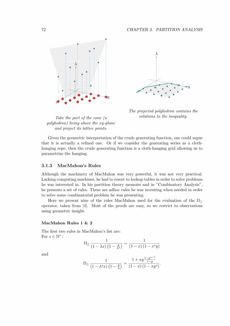
72 CHAPTER 3. PARTITION ANALYSIS
𝑥𝑦
𝜆
Take the part of the cone (apolyhedron) living above the 𝑥𝑦-plane
and project its lattice points.
𝑥𝑦
𝜆
The projected polyhedron contains thesolutions to the inequality.
Given the geometric interpretation of the crude generating function, one could arguethat it is actually a refined one. Or if we consider the generating series as a cloth-hanging rope, then the crude generating function is a cloth-hanging grid allowing us toparametrize the hanging.
3.1.3 MacMahon’s Rules
Although the machinery of MacMahon was very powerful, it was not very practical.Lacking computing machines, he had to resort to lookup tables in order to solve problemshe was interested in. In his partition theory memoirs and in ”Combinatory Analysis”,he presents a set of rules. These are adhoc rules he was inventing when needed in orderto solve some combinatorial problem he was presenting.
Here we present nine of the rules MacMahon used for the evaluation of the Ω≥operator, taken from [4]. Most of the proofs are easy, so we restrict to observationsusing geometric insight.
MacMahon Rules 1 & 2
The first two rules in MacMahon’s list are:For 𝑠 ∈ N* :
Ω≥1
(1− 𝜆𝑥)(1− 𝑦
𝜆𝑠
) =1
(1− 𝑥) (1− 𝑥𝑠𝑦)
and
Ω≥1
(1− 𝜆𝑠𝑥)(1− 𝑦
𝜆
) =1 + 𝑥𝑦 1−𝑦𝑠−1
1−𝑦
(1− 𝑥) (1− 𝑥𝑦𝑠).
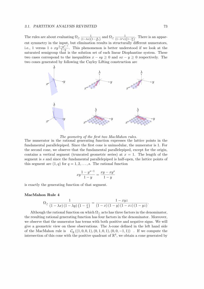
3.1. PARTITION ANALYSIS REVISITED 73
The rules are about evaluating Ω≥1
(1−𝜆𝑥)(1− 𝑦𝜆𝑠 )
and Ω≥1
(1−𝜆𝑠𝑥)(1− 𝑦𝜆)
. There is an appar-
ent symmetry in the input, but elimination results in structurally different numerators,
i.e., 1 versus 1 + 𝑥𝑦 1−𝑦𝑠−1
1−𝑦 . This phenomenon is better understood if we look at thesaturated semigroup that is the solution set of each linear Diophantine system. Thesetwo cases correspond to the inequalities 𝑥 − 𝑠𝑦 ≥ 0 and 𝑠𝑥 − 𝑦 ≥ 0 respectively. Thetwo cones generated by following the Cayley Lifting construction are
𝑥𝑦
𝜆
𝑥
𝑦
𝜆
𝑥
𝑦
𝜆
𝑥𝑦
𝜆
𝑥𝑦
𝜆
𝑥𝑦
𝜆
The geometry of the first two MacMahon rules.The numerator in the rational generating function expresses the lattice points in thefundamental parallelepiped. Since the first cone is unimodular, the numerator is 1. Forthe second cone, we observe that the fundamental parallelepiped, except for the origin,contains a vertical segment (truncated geometric series) at 𝑥 = 1. The length of thesegment is 𝑠 and since the fundamental parallelepiped is half-open, the lattice points ofthis segment are (1, 𝑞) for 𝑞 = 1, 2, . . . , 𝑠. The rational function
𝑥𝑦1− 𝑦𝑠−1
1− 𝑦=
𝑥𝑦 − 𝑥𝑦𝑠
1− 𝑦
is exactly the generating function of that segment.
MacMahon Rule 4
Ω≥1
(1− 𝜆𝑥) (1− 𝜆𝑦)(1− 𝑧
𝜆
) =1− 𝑥𝑦𝑧
(1− 𝑥) (1− 𝑦) (1− 𝑥𝑧) (1− 𝑦𝑧).
Although the rational function on which Ω≥ acts has three factors in the denominator,the resulting rational generating function has four factors in the denominator. Moreover,we observe that the numerator has terms with both positive and negative signs. We willgive a geometric view on these observations. The 𝜆-cone defined in the left hand sideof the MacMahon rule is 𝒞R ((1, 0, 0, 1), (0, 1, 0, 1), (0, 0,−1, 1)) . If we compute theintersection of this cone with the positive quadrant of R4, we obtain a cone generated by

74 CHAPTER 3. PARTITION ANALYSIS
(1, 0, 0, 1), (0, 1, 0, 1), (1, 0, 1, 0) and (0, 1, 1, 0). Let’s project this into R3 (by eliminatingthe last coordinate). We obtain a non-simplicial cone. We provide two decompositionsof the cone into simplicial cones. We used Normaliz [21] for the computations.
The first decomposition is by triangulation as shown here:
𝑥𝑦
𝑧
𝑥
𝑦
𝑧
𝑥
𝑦
𝑧
𝑥
𝑦
𝑧
𝑥
𝑦
𝑧
The generating function of the green cone 𝒞R ((1, 0, 0), (0, 1, 0), (1, 0, 1)) is
1
(1− 𝑥) (1− 𝑦) (1− 𝑥𝑧)
while that of the red cone 𝒞R ((0, 1, 0), (0, 1, 1), (1, 0, 1)) is
1
(1− 𝑦) (1− 𝑥𝑧) (1− 𝑦𝑧).
If we perform inclusion-exclusion (subtracting the purple cone), we obtain:
1
(1− 𝑥) (1− 𝑦) (1− 𝑥𝑧)+
1
(1− 𝑦) (1− 𝑥𝑧) (1− 𝑦𝑧)− 1
(1− 𝑦) (1− 𝑥𝑧)=
(1− 𝑥𝑦) (1− 𝑦)
(1− 𝑥) (1− 𝑦) (1− 𝑥𝑧) (1− 𝑦𝑧)− 1
(1− 𝑦) (1− 𝑥𝑧)=
(1− 𝑥𝑦) (1− 𝑦)− (1− 𝑥𝑧)
(1− 𝑦) (1− 𝑦) (1− 𝑥𝑧) (1− 𝑦𝑧)=
1− 𝑥𝑦𝑧
(1− 𝑦) (1− 𝑦) (1− 𝑥𝑧) (1− 𝑦𝑧)
The second decomposition is not a triangulation, but a signed cone decomposition (a laBarvinok).
𝑥𝑦
𝑧
𝑥
𝑦
𝑧
𝑥
𝑦
𝑧
𝑥
𝑦
𝑧
We first consider the whole positive quadrant and then subtract the half-open cone
𝒞(0,0,1)R ((1, 0, 1), (0, 1, 1), (0, 0, 1)) . Half-opening the cone is equivalent (as far as latticepoints are concerned) to shifting the cone by the generator (0, 0, 1). Thus we have atthe generating function level:

3.1. PARTITION ANALYSIS REVISITED 75
1
(1− 𝑥) (1− 𝑦) (1− 𝑧)− 𝑧
(1− 𝑥𝑧) (1− 𝑦𝑧) (1− 𝑧)=
(1− 𝑥𝑧) (1− 𝑦𝑧)− 𝑧 (1− 𝑥) (1− 𝑦)
(1− 𝑥) (1− 𝑦) (1− 𝑧) (1− 𝑥𝑧) (1− 𝑦𝑧)=
(1− 𝑧)− 𝑥𝑦𝑧 (1− 𝑧)
(1− 𝑦) (1− 𝑦) (1− 𝑧) (1− 𝑥𝑧) (1− 𝑦𝑧)=
1− 𝑥𝑦𝑧
(1− 𝑦) (1− 𝑦) (1− 𝑥𝑧) (1− 𝑦𝑧)
MacMahon Rule 6
Ω≥1
(1− 𝜆2𝑥)(1− 𝑦
𝜆
) (1− 𝑧
𝜆
) =1 + 𝑥𝑦 + 𝑥𝑧 + 𝑥𝑦𝑧
(1− 𝑥) (1− 𝑥𝑦2) (1− 𝑥𝑧2).
In this rule we observe that we have a positive sum of four terms in the numerator.The Ω-polyhedron is a cone that is simplicial but not unimodular. Observe in the figurethe four points in the fundamental parallelepiped, corresponding to the four terms in
the sum.
𝑥
𝑦
𝑧
𝑥
𝑦
𝑧
Other MacMahon Rules
Although the list of rules is not comprehensive, in the sense that they cannot cover allcases needed to treat linear Diophantine systems, they can solve certain combinatorialproblems. For the rest of MacMahon’s rules similar geometric observations apply, butthe geometry becomes more complicated and the reasoning behind the numerators orthe denominators appearing is not as simple anymore. A list of other MacMahon rulesis given here:
MacMahon Rule 3
Ω≥1
(1− 𝜆𝑥)(1− 𝑦
𝜆
) (1− 𝑧
𝜆
) =1
(1− 𝑥) (1− 𝑥𝑦) (1− 𝑥𝑧).

76 CHAPTER 3. PARTITION ANALYSIS
MacMahon Rule 5
Ω≥1
(1− 𝜆𝑥) (1− 𝜆𝑦)(1− 𝑧
𝜆2
) =1 + 𝑥𝑦𝑧 − 𝑥2𝑦𝑧 − 𝑥𝑦2𝑧
(1− 𝑥) (1− 𝑦) (1− 𝑥2𝑧) (1− 𝑦2𝑧).
MacMahon Rule 7
Ω≥1
(1− 𝜆2𝑥) (1− 𝜆𝑦)(1− 𝑧
𝜆
) =1 + 𝑥𝑧 − 𝑥𝑦𝑧 − 𝑥𝑦𝑧2
(1− 𝑥) (1− 𝑦) (1− 𝑦𝑧) (1− 𝑥𝑧2).
MacMahon Rule 8
1
(1− 𝜆𝑥) (1− 𝜆𝑦) (1− 𝜆𝑧)(1− 𝑤
𝜆
) =
1− 𝑥𝑦𝑤 − 𝑥𝑧𝑤 − 𝑦𝑧𝑤 + 𝑥𝑦𝑧𝑤 + 𝑥𝑦𝑧𝑤2
(1− 𝑥) (1− 𝑦) (1− 𝑧) (1− 𝑥𝑤) (1− 𝑦𝑤) (1− 𝑧𝑤).
MacMahon Rule 9
Ω≥1
(1− 𝜆𝑥) (1− 𝜆𝑦)(1− 𝑧
𝜆
) (1− 𝑤
𝜆
) =
1− 𝑥𝑦𝑧 − 𝑥𝑦𝑤 − 𝑥𝑦𝑧𝑤 + 𝑥𝑦2𝑧𝑤 + 𝑥2𝑦𝑧𝑤
(1− 𝑥) (1− 𝑦) (1− 𝑥𝑧) (1− 𝑥𝑤) (1− 𝑦𝑧) (1− 𝑦𝑤).
3.1.4 Andrews-Paule-Riese
In 1997, Bousquet–Melou and Eriksson presented a theorem on lecture-hall partitionsin [18]. This theorem gathered a lot of attention from the community (and it stilldoes, with many lecture-hall type theorems appearing still today). Andrews, who hadalready studied MacMahon’s method and was aware of its computational potential,figured that lecture-hall partitions offered the right problems to attack algorithmicallyvia partition analysis. At the same time he planned to spend a semester during hissabbatical at the Research Institute for Symbolic Computation (RISC) in Austria towork with Paule. It is only natural that the result was a fully algorithmic versionof MacMahon’s method powered by symbolic computation. This collaboration gavea series of 10 papers [4, 1, 10, 5, 6, 7, 3, 8, 9, 2]. Many interesting theorems anddifferent kinds of partitions are defined and explored in this series, but for us the twomost important references are [4] and [5], which contain the algorithmic improvementson partition analysis. Namely, in [4] the authors introduce Omega, a Mathematicapackage based on a fully algorithmic partition analysis version, while in [5] they presenta more advanced partial fraction decomposition (and the related Mathematica packageOmega2) solving some of the problems appearing in Omega. While presenting the twomethods, we will see some geometric aspects of theirs.

3.1. PARTITION ANALYSIS REVISITED 77
Omega
The main tool in Omega is the Fundamental Recurrence for the Ω≥ operator, given byLemma 6. Following MacMahon, or Elliott for that matter, iterative application of thisrecurrence is enough for computing the action of Ω≥.
Lemma 6 (Fundamental Recurrence, Theorem 2.1 in [4]). For 𝑚,𝑛 ∈ N* and 𝑎 ∈ Z:
Ω≥𝜆𝑎
(1− 𝑥1𝜆) · · · (1− 𝑥𝑛𝜆)(1− 𝑦1𝜆 ) · · · (1− 𝑦𝑚
𝜆 )=
𝑃𝑛,𝑚,𝑎(𝑥1, 𝑥2, . . . , 𝑥𝑛; 𝑦1, 𝑦2, . . . , 𝑦𝑚)∏𝑛𝑖=1(1− 𝑥𝑖)
∏𝑛𝑖=1
∏𝑚𝑗=1(1− 𝑥𝑖𝑦𝑗)
where for 𝑛 > 1
𝑃𝑛,𝑚,𝑎(𝑥1, . . . , 𝑥𝑛; 𝑦1, . . . , 𝑦𝑚) =
1
𝑥𝑛 − 𝑥𝑛−1
⎛⎝𝑥𝑛(1− 𝑥𝑛−1)
𝑚∏𝑗=1
(1− 𝑥𝑛−1𝑦𝑗)𝑃𝑛−1,𝑚,𝑎(𝑥1, . . . , 𝑥𝑛−2, 𝑥𝑛; 𝑦1, . . . , 𝑦𝑚)
−𝑥𝑛−1(1− 𝑥𝑛)𝑚∏𝑗=1
(1− 𝑥𝑛𝑦𝑗)𝑃𝑛−1,𝑚,𝑎(𝑥1, . . . , 𝑥𝑛−2, 𝑥𝑛−1; 𝑦1, . . . , 𝑦𝑚)
⎞⎠and for 𝑛 = 1
𝑃1,𝑚,𝑎(𝑥1; 𝑦1, . . . , 𝑦𝑚) =
⎧⎪⎨⎪⎩𝑥−𝑎1 if 𝑎 ≤ 0
𝑥−𝑎1 +
𝑚∏𝑗=1
(1− 𝑥1𝑦𝑗)𝑎∑
𝑗=0
ℎ𝑗(𝑦1, . . . , 𝑦𝑚)(1− 𝑥𝑗−𝑎1 ) if 𝑎 > 0
�
The recurrence looks intimidating, but bear in mind that it is supposed to be a computa-tional tool used in combination with symbolic computation. It is this power that earlierauthors did not have. Even the ones with extreme computational (by hand) abilities,like MacMahon, had to resort to lookup tables and sets of rules for the more usual cases.
The base cases for the recurrence are when either all the terms have positive 𝜆-exponents or all the terms have negative-𝜆 exponents. For the two base cases we recall thedefinition of complete homogeneous symmetric polynomials and some related notation.
Definition 3.2 (Complete Homogeneous Symmetric Polynomials, see [5])We define ℎ𝑖(𝑧1, 𝑧2, . . . , 𝑧𝑛) through the generating function
∞∑𝑖=0
ℎ𝑖(𝑧1, 𝑧2, . . . , 𝑧𝑛)𝑡𝑖 =
1
(1− 𝑧1𝑡)(1− 𝑧2𝑡) · · · (1− 𝑧𝑛𝑡).
What is needed for the base cases of the fundamental recurrence, is the partial sum ofthis generating function (series). The following definition is useful to set notation.

78 CHAPTER 3. PARTITION ANALYSIS
For 𝑎 ∈ Z, let
𝐻𝑎(𝑧1, 𝑧2, . . . , 𝑧𝑛) =
{∑𝑎𝑖=0 ℎ𝑖(𝑧1, 𝑧2, . . . , 𝑧𝑛) if 𝑎 ≥ 0
0 if 𝑎 < 0.
�
Now, returning to [4], we have the two base cases:
Lemma 7 (Lemma 2.1 in [4]). For any integer 𝑎,
Ω≥𝜆𝛼
(1− 𝑥1𝜆)(1− 𝑥2𝜆) . . . (1− 𝑥𝑛𝜆)= Ω≥
∞∑𝑗=0
ℎ𝑗(𝑥1, 𝑥2, . . . , 𝑥𝑛)𝜆𝑎+𝑗
= 1(1−𝑥1)(1−𝑥2)...(1−𝑥𝑛)
−𝐻−𝑎−1(𝑥1, 𝑥2, . . . , 𝑥𝑛).�
Lemma 8 (Lemma 2.2 in [4]). For any integer 𝑎,
Ω≥𝜆𝛼
(1− 𝑦1𝜆 )(1− 𝑦2
𝜆 ) . . . (1− 𝑦𝑚𝜆 )
= Ω≥
∞∑𝑗=0
ℎ𝑗(𝑦1, 𝑦2, . . . , 𝑦𝑚)𝜆𝑎−𝑗
= 𝐻𝑎(𝑥1, 𝑥2, . . . , 𝑥𝑛). �
The fundamental recurrence in Lemma 6 assumes that the exponents of 𝜆 in thedenominator are ±1. This is not a strong assumption, as noted in [4], since we canalways employ the following decomposition.
(1− 𝑥𝜆𝑟) =
𝑟−1∏𝑗=0
(1− 𝜌𝑗𝑥1𝑟𝜆)
(1− 𝑦
𝜆𝑠) =
𝑠−1∏𝑗=0
(1− 𝜎𝑗𝑦1𝑠
𝜆)
where 𝜌 = 𝑒2𝜋𝑖𝑟 and 𝜎 = 𝑒
2𝜋𝑖𝑠 . The obvious drawback of this approach is that we introduce
complex coefficients instead of just ±1, which were the only possible coefficients beforethe decomposition. This motivates the desire for a better recurrence.
Omega2
In [5] the authors introduce an improved partial fraction decomposition method, givenby the recurrence of Theorem 3.1.
Theorem 3.1 (Generalized Partial Fraction Decomposition, see [5])Let 𝛼 ≥ 𝛽 ≥ 1, gcd(𝛼, 𝛽) = 1 and let rmd(𝑎, 𝑏) denote the division remainder of 𝑎 by 𝑏.Then
1
(1− 𝑧1𝑧𝛼3 )(1− 𝑧2𝑧𝛽3 )
=1
(𝑧𝛼2 − 𝑧𝛽1 )
(𝑃 (𝑧3)
(1− 𝑧1𝑧𝛼3 )+
��(𝑧3)
(1− 𝑧2𝑧𝛽3 )
)(3.8)

3.1. PARTITION ANALYSIS REVISITED 79
where
𝑃 (𝑧3) :=𝛼−1∑𝑖=0
��𝑖𝑧𝑖3 for 𝑎𝑖 =
⎧⎨⎩−𝑧𝛽1 𝑧𝑖𝛽
2 if 𝛽|𝑖 or 𝑖 = 0,
−𝑧rmd((𝛼−1 mod 𝛽)𝑖,𝛽)1 𝑧
rmd((𝛽−1 mod 𝛼)𝑖,𝛼)2 otherwise,
while
��(𝑧3) :=
𝛽−1∑𝑖=0
��𝑖𝑧𝑖3 for ��𝑖 =
{𝑧𝛼2 if 𝑖 = 0,
𝑧rmd((𝛼−1 mod 𝛽)𝑖,𝛽)1 𝑧
rmd((𝛽−1 mod 𝛼)𝑖,𝛼)2 otherwise.
�
Moreover, two new base cases are introduced. As before, we define some notation forhomogeneous polynomials.
Definition 3.3 (Oblique Complete Homogeneous Polynomials, see [5])For 𝜁1, 𝜁2, . . . , 𝜁𝑛 ∈ N*, we define ℎ𝑖(𝑧1, 𝑧2, . . . , 𝑧𝑛; 𝜁1, 𝜁2, . . . , 𝜁𝑛) through the generatingfunction
∞∑𝑖=0
ℎ𝑖(𝑧1, 𝑧2, . . . , 𝑧𝑛; 𝜁1, 𝜁2, . . . , 𝜁𝑛)𝑡𝑖 =
1
(1− 𝑧1𝑡𝜁1)(1− 𝑧2𝑡𝜁2) · · · (1− 𝑧𝑛𝑡𝜁𝑛).
�
The related partial sums are defined for 𝑎 ∈ Z, as
𝐻𝑎(𝑧1, 𝑧2, . . . , 𝑧𝑛; 𝜁1, 𝜁2, . . . , 𝜁𝑛) =
{∑𝑎𝑖=0 ℎ𝑖(𝑧1, 𝑧2, . . . , 𝑧𝑛; 𝜁1, 𝜁2, . . . , 𝜁𝑛) if 𝑎 ≥ 0
0 if 𝑎 < 0.
Lemma 9 (Case 𝑚 = 0, Section 2 in [5]). For any integer 𝑎,
Ω≥𝜆𝑎
(1− 𝑥1𝜆𝑗1)(1− 𝑥2𝜆𝑗2) . . . (1− 𝑥𝑛𝜆𝑗𝑛)= Ω≥
∞∑𝑗=0
ℎ𝑗(𝑥1, 𝑥2, . . . , 𝑥𝑛; 𝑗1, 𝑗2, . . . , 𝑗𝑛)𝜆𝑎+𝑗
=1
(1− 𝑥1)(1− 𝑥2) . . . (1− 𝑥𝑛)
−𝐻−𝑎−1(𝑥1, 𝑥2, . . . , 𝑥𝑛; 𝑗1, 𝑗2, . . . , 𝑗𝑛).
�
Lemma 10 (Case 𝑛 = 0, Section 2 in [5]). For any integer 𝑎,
Ω≥𝜆𝑎
(1− 𝑦1𝜆𝑗1
)(1− 𝑦2𝜆𝑗2
) . . . (1− 𝑦𝑚𝜆𝑗𝑚 )
= Ω≥
∞∑𝑗=0
ℎ𝑗(𝑥1, 𝑥2, . . . , 𝑥𝑛; 𝑗1, 𝑗2, . . . , 𝑗𝑛)𝜆𝑎−𝑗
= 𝐻𝑎(𝑥1, 𝑥2, . . . , 𝑥𝑛; 𝑗1, 𝑗2, . . . , 𝑗𝑛).
�

80 CHAPTER 3. PARTITION ANALYSIS
Lemma 11 (Case 𝑚 = 1, Section 2 in [5]). For any integer 𝑎 < 𝑗,
Ω≥𝜆𝑎
(1− 𝑥1𝜆𝑗1) . . . (1− 𝑥𝑛𝜆𝑗𝑛)(1− 𝑦𝜆−𝑘)=
1
(1− 𝑥1)(1− 𝑥2) . . . (1− 𝑥𝑛)(1− 𝑦)
−∑𝑘−1
𝜏1,𝜏2,...,𝜏𝑛=0
∏𝑥𝜏𝑖𝑖 𝑦
⌊∑𝑗𝑖𝜏𝑖+𝑎
𝑘
⌋+1
(1− 𝑥𝑘1𝑦𝑗1) . . . (1− 𝑥𝑘𝑛𝑦
𝑗𝑛)(1− 𝑦).
�
Lemma 12 (Case 𝑛 = 1, Section 2 in [5]). For any integer 𝑎 > −𝑘,
Ω≥𝜆𝑎
(1− 𝑥𝜆𝑗)(1− 𝑦1𝜆−𝑘1) . . . (1− 𝑦𝑚𝜆−𝑘𝑚)=
∑𝑗−1𝜏1,𝜏2,...,𝜏𝑛=0
∏𝑦𝜏𝑖𝑖 𝑥
⌈∑𝑘𝑖𝜏𝑖−𝑎
𝑗
⌉(1− 𝑥)(1− 𝑥𝑘1𝑦𝑗1) . . . (1− 𝑥𝑘𝑚𝑦𝑗𝑚)
.
�
Omega2 was used to obtain results in a series of papers by Andrews-Paule andtheir coauthors, dealing with various problems from partition theory. For the project ingeneral see http://www.risc.jku.at/research/combinat/software/Omega/.
Now we proceed with the geometric interpretation of the Generalized Partial FractionDecomposition. We first rewrite (3.8) by pulling out −𝑧𝛽1 from the denominator of
1
(𝑧𝛼2 −𝑧𝛽1 ),i.e.,
1
(1− 𝑧1𝑧𝛼3 )(1− 𝑧2𝑧𝛽3 )
=−𝑧−𝛽
1 𝑃 (𝑧3)
(1− 𝑧−𝛽1 𝑧𝛼2 )(1− 𝑧1𝑧𝛼3 )
− 𝑧−𝛽1 ��(𝑧3)
(1− 𝑧−𝛽1 𝑧𝛼2 )(1− 𝑧2𝑧
𝛽3 )
, (3.9)
and define 𝑃𝛼,𝛽 and 𝑄𝛼,𝛽 to be
∙ 𝑃𝛼,𝛽 := −𝑧−𝛽1 𝑃 (𝑧3) =
∑𝛼−1𝑖=0 𝑎𝑖𝑧
𝑖3
∙ 𝑄𝛼,𝛽 := 𝑧−𝛽1 ��(𝑧3) =
∑𝛽−1𝑖=0 𝑏𝑖𝑧
𝑖3
where
∙ 𝑎𝑖 =
⎧⎨⎩𝑧𝑖𝛽
2 if 𝛽|𝑖 or 𝑖 = 0,
𝑧rmd((𝛼−1 mod 𝛽)𝑖,𝛽)−𝛽1 𝑧
rmd((𝛽−1 mod 𝛼)𝑖,𝛼)2 otherwise,
∙ 𝑏𝑖 =
{𝑧−𝛽1 𝑧𝛼2 if 𝑖 = 0,
𝑧rmd((𝛼−1 mod 𝛽)𝑖,𝛽)−𝛽1 𝑧
rmd((𝛽−1 mod 𝛼)𝑖,𝛼)2 otherwise.
The following theorem provides the basis for the geometric interpretation of theGeneralized Partial Fraction Decomposition.

3.1. PARTITION ANALYSIS REVISITED 81
Theorem 3.2 (Polyhedral geometry interpretation of Omega2)Application of the generalized partial fraction decomposition
1
(1− 𝑧1𝑧𝛼3 )(1− 𝑧2𝑧𝛽3 )
=𝑃𝛼,𝛽
(1− 𝑧−𝛽1 𝑧𝛼2 )(1− 𝑧1𝑧𝛼3 )
−𝑄𝛼,𝛽
(1− 𝑧−𝛽1 𝑧𝛼2 )(1− 𝑧2𝑧
𝛽3 )
(3.10)
on 𝜌𝐶(z) induces a signed cone decomposition 1 of the cone 𝐶 = 𝒞R ((1, 0, 𝛼), (0, 1, 𝛽)).�
Proof Strategy:
∙ Determine the structure of the fundamental parallelepiped of the cones 𝐴 =𝒞R ((−𝛽, 𝛼, 0), (1, 0, 𝛼)) and 𝐵 = 𝒞R ((−𝛽, 𝛼, 0), (0, 1, 𝛽)).
∙ Prove that 𝑃𝛼,𝛽 and 𝑄𝛼,𝛽 are the generating functions of these fundamental par-allelepipeds.
For the detailed proof of Theorem 3.2 see Appendix A. Here we provide the pic-ture of the decomposition for the cone 𝐶 = 𝒞R ((1, 0, 3), (0, 1, 5)), into the cones 𝐴 =
𝒞R ((−5, 3, 0), (1, 0, 3)) and 𝐵 = 𝒞0,1R ((−5, 3, 0), (0, 1, 5)).
𝑥
𝑦
𝑧(1, 0, 3)
(0, 1, 5) 𝑥
𝑦
𝑧
(−5, 3, 0)
(1, 0, 3)(0, 1, 5)
1A decomposition into a sum where the summands may have positive or negative sign.

82 CHAPTER 3. PARTITION ANALYSIS
𝑥
𝑦
𝑧(1, 0, 3)
(−5, 3, 0)
(0, 1, 5)𝑥
𝑦
𝑧(1, 0, 3)
(−5, 3, 0)
(0, 1, 5)
The statement (from the proof in Appendix A)
𝜌Π(𝐵) = 𝑄𝛼,𝛽 + 1− 𝑧−𝛽1 𝑧𝛼2
means that𝑄𝛼,𝛽
(1−𝑧−𝛽1 𝑧𝛼2 )(1−𝑧2𝑧
𝛽3 )
is the generating function of the half-open cone 𝐵 that is
open on the ray generated by (−𝛽, 𝛼, 0).One can see the full signed decomposition on the generating-function level as follows:
𝜌𝐶 = 𝜌𝐴 − 𝜌𝐵 + 𝜌𝒞R((0,1,𝛽)).
According to the previous analysis 𝜌𝐴 =𝑃𝛼,𝛽
(1−𝑧−𝛽1 𝑧𝛼2 )(1−𝑧1𝑧𝛼3 )
.
Since 𝜌𝒞R((0,1,𝛽))= 1
(1−𝑧2𝑧𝛽3 )
we have
−𝜌𝐵 + 𝜌𝒞R((0,1,𝛽))= −
𝑄𝛼,𝛽 + 1− 𝑧−𝛽1 𝑧𝛼2
(1− 𝑧−𝛽1 𝑧𝛼2 )(1− 𝑧2𝑧
𝛽3 )
+1(
1− 𝑧2𝑧𝛽3
)= −
𝑄𝛼,𝛽
(1− 𝑧−𝛽1 𝑧𝛼2 )(1− 𝑧2𝑧
𝛽3 )
which means
1
(1− 𝑧1𝑧𝛼3 )(1− 𝑧2𝑧𝛽3 )
=𝑃𝛼,𝛽
(1− 𝑧−𝛽1 𝑧𝛼2 )(1− 𝑧1𝑧𝛼3 )
−𝑄𝛼,𝛽
(1− 𝑧−𝛽1 𝑧𝛼2 )(1− 𝑧2𝑧
𝛽3 )
.
In other words, 𝑄𝛼,𝛽 encodes the inclusion-exclusion step in the decomposition.

3.2. ALGEBRAIC PARTITION ANALYSIS 83
3.2 Algebraic Partition Analysis
Having reviewed the history of partition analysis both from the perspective of the originalauthors and from a more geometric perspective, we give now an algebraic presentationthe Ω≥ operator .
In particular, we will use graded vector spaces and rings in order to compute thegenerating functions of the solutions of a linear Diophantine system.
3.2.1 Graded Rings
Let 𝑅 = K [𝑧1, 𝑧2, . . . , 𝑧𝑑] be the ring of polynomials in 𝑑 variables 𝑧1, 𝑧2, . . . , 𝑧𝑑. In whatfollows we will grade this ring in a way that is useful for solving linear Diophantinesystems. Let us first define a graded vector space, as we will look at the polynomial ringas a vector space over the coefficient field.
Definition 3.4 (Graded vector space)Let K be a field and 𝑉 a vector space of K. If there exists a direct sum decomposition
𝑉 =⨁𝑖∈𝐼
𝑉𝑖
of 𝑉 into linear subspaces 𝑉𝑖 for some index set 𝐼, then we say that 𝑉 is 𝐼-gradedand the 𝑉𝑖’s are called homogeneous components, while the elements of 𝑉𝑘 are calledhomogeneous elements of degree 𝑘. �
The most usual grading of the polynomial ring K [𝑧1, 𝑧2, . . . , 𝑧𝑑] is the one inducedby the usual polynomial degree. The homogeneous component 𝑉𝑘 is the linear span ofall monomials of degree 𝑘, i.e., the set of all homogeneous polynomials of degree 𝑘 andthe polynomial 0.
A notion that connects graded algebraic structures with generating functions is thatof the Hilbert-Poincare series. Given a graded vector space 𝑉 =
⨁𝑖∈𝐼 𝑉𝑖 for some
(appropriate) index set 𝐼, then the Hilbert-Poincare series of 𝑉 over K is the formalpowerseries
ℋ𝒫 (𝑉 ) =∑𝑖∈𝐼
dimK (𝑉𝑖) 𝑡𝑖.
Note that:
∙ The most usual definition of Hilbert-Poincare series in the literature, restricts theindex set 𝐼 to be N and all linear subspaces 𝑉𝑖 to be finite-dimensional.
∙ If the index set 𝐼 is not a subset of N𝑘 for some 𝑘, but all elements of 𝐼 are boundedfrom below, then the Hilbert-Poincare series is a formal Laurent series. If the indexset contains elements that are not bounded from below, then the Hilbert-Poincareseries is not defined.
∙ According to the definition of a graded vector space, it is possible that not all 𝑉𝑖
are finite-dimensional. In that case the Hilbert-Poincare series is not defined.

84 CHAPTER 3. PARTITION ANALYSIS
The algebraic approach to partition analysis has its roots in the very early work andmotivation of Cayley, MacMahon and Elliott. Their motivation to deal with the problemstem from invariant theory, which was very fashionable these days. We will present herea setup of algebraic structures and associated series, mostly Hilbert series, which allowsto view partition analysis algebraically. In the definition of graded vector spaces, andas is customary in literature, we first defined the homogeneous components and thenassign to the elements of each component the corresponding degree. For our purposesthough, it is more natural to follow the reverse path. We will first define a degree onthe elements of the polynomial ring and then construct the homogeneous components asthe linear span of all elements of the same degree. In particular, we want to constructa grading of K [𝑧1, 𝑧2, . . . , 𝑧𝑑] starting from a matrix 𝐴 in Z𝑚×𝑑. We assume that 𝐴 isfull-rank.
Let 𝑓𝑎𝑖 be the linear functionals defined by the rows of 𝐴 for 𝑖 ∈ [𝑚]. We define thefunction 𝐹 : N𝑑 ↦→ Z𝑚 by
𝐹 (𝑣) = (𝑓𝑎1(𝑣), 𝑓𝑎2(𝑣), . . . , 𝑓𝑎𝑚(𝑣)) for 𝑣 ∈ N𝑑.
Since we want to use this function to grade the polynomial ring, it is necessary totranslate from vectors to monomials and back. Given a set of formal variables 𝑍 ={𝑧1, 𝑧2, . . . , 𝑧𝑑}, we define the term monoid T to be the subset of K [𝑧1, 𝑧2, . . . , 𝑧𝑑] con-sisting of powerproducts, i.e., {𝑧𝑎11 𝑧𝑎22 · · · 𝑧
𝑎𝑑𝑑 |𝑎𝑖 ∈ N} and we set 1 = 𝑧0. This is a
multiplicative monoid with the standard monomial multiplication. We define 𝜑 as
𝜑 :N𝑑 → T𝑣 ↦→ 𝑧𝑣
establishing the monoid isomorphism N𝑑 ≃ T. Now, we can define a degree in T via 𝐹 .
N𝑑
T Z𝑚
≃ 𝐹
deg
In words, let deg : T→ Z𝑚 be defined as deg(𝑧𝑣) = 𝐹(𝜑−1(𝑧𝑣)
).
Define 𝑉𝑖 for 𝑖 ∈ Z𝑚 to be the linear span over K of all elements in T with degree 𝑖, i.e.,
𝑉𝑖 =
{𝑛∑
𝑘=0
𝑐𝑘𝑡𝑘
𝑛 ∈ N, 𝑐𝑘 ∈ K, 𝑡𝑘 ∈ T with deg 𝑡𝑘 = 𝑖
}for 𝑖 ∈ Z𝑚
= ⟨𝑡 ∈ T : deg(𝑡) = 𝑖⟩K, for 𝑖 ∈ Z𝑚
and ⟨∅⟩K = {0}. Then we have that
ℛ = ⊕𝑖∈Z𝑚𝑉𝑖.
This means that the collection of 𝑉𝑖’s defines a grading on K [𝑧1, 𝑧2, . . . , 𝑧𝑑], which nowcan be seen as a graded vector space. Let us see an example of such a grading.

3.2. ALGEBRAIC PARTITION ANALYSIS 85
Example 9 (Total degree or ℓ1-grading). The degree function is given by 𝐹 (𝑠) = |𝑠|1,i.e., the matrix 𝐴 is the unit matrix of rank 𝑑. This is the usual total degree for polyno-mials in 𝑑 variables. In the figure we see the grading for 𝑑 = 2.
10
9
8
7
6
0 1 2 3 4 5
𝑉𝑖 is the vector space of homogeneous polynomials of degree 𝑖.
�
Example 10. Let the degree map be defined by 𝐹 (𝑠) = 𝑠. The grading this map inducesis called trivial because each K-vector space 𝑉𝑎 is generated by 𝑧𝑎 alone.
�
We note that some (or all) 𝑉𝑖 may be infinite dimensional depending on the matrix 𝐴we started with, as in the following example.
Example 11. Let the degree map be defined by 𝐹 (𝑥, 𝑦) = 𝑥 − 𝑦. The grading thismap induces is infinite, because each K-vector space 𝑉𝑖 is generated by infinitely manymonomials.

86 CHAPTER 3. PARTITION ANALYSIS
−1−2−3−4−5 0
1
2
3
4
5
�
The Hilbert-Poincare series provide a useful, refined counting tool for the numberof solutions of linear Diophantine systems. Nevertheless, we would like to allow fornon finite-dimensional graded components as well as for a tool enumerating rather thancounting solutions.
Each 𝑉𝑖 is a vector space containing homogeneous polynomials of degree 𝑖. It is alwayspossible to pick a basis of 𝑉𝑖 consisting of terms of degree 𝑖, i.e., elements of T. We willdenote such a basis by ℬ𝑖. We define the basis of {0} to be the empty set.
In the direction of obtaining an enumerating generating function we define the trun-cated multivariate Hilbert-Poincare series,
Definition 3.5 (truncated multivariate Hilbert-Poincare series)Given a graded vector space 𝑉 =
⨁𝑖∈Z𝑘 𝑉𝑖 over the field K and a vector 𝑏 ∈ Z𝑘 for some
𝑘 ∈ N, we define the truncated multivariate Hilbert-Poincare series of 𝑉 as
𝑡ℋ𝒫𝑉𝑏 (𝑧, 𝑡) =
∑𝑏≤𝑖∈Z𝑘
⎛⎝∑𝑒∈ℬ𝑖
𝑒
⎞⎠ 𝑡𝑖.
The truncated multivariate Hilbert-Poincare series is a formal Laurent series in the 𝑡variables and a formal powerseries in the 𝑧 variables. �
The truncation in the indices is necessary in order to ensure that the formal Laurentseries is well defined, while the formal sum of the basis elements avoid the problem ofinfinite-dimensionality. At the same time, this formal series enumerates all solutions ofa linear Diophantine system 𝐴𝑥 ≥ 𝑏, if the vector space 𝑉 is graded via the proceduredescribed above for the matrix 𝐴 ∈ Z𝑚×𝑑. We note that in that case 𝑘 = 𝑚.
The following theorem provides the connection between the Ω≥ operator and Hilbert-Poincare series.
3.2. ALGEBRAIC PARTITION ANALYSIS 87
Theorem 1. Given 𝐴 ∈ Z𝑚×𝑑, 𝑏 ∈ Z𝑚 and 𝑡ℋ𝒫𝑉𝑏 (𝑧, 𝑡) as above, we have
Ω≥∑𝑥∈N𝑛
𝑧𝑥𝑚∏𝑖=1
𝜆𝐴𝑖𝑥−𝑏𝑖𝑖 = 𝑡ℋ𝒫𝑉
𝑏 (𝑧, 𝑡)|𝑡=1.
�
Proof. Let 𝑆 be the set of solutions to the linear Diophantine system 𝐴𝑥 ≥ 𝑏. By thedefinition of the Ω≥ operator, we have that Ω≥
∑x∈N𝑛 zx
∏𝑚𝑖=1 𝜆
𝐴𝑖x−𝑏𝑖𝑖 is Φ𝐴,𝑏(𝑧), the
generating function of 𝑆. Now we have:
𝛼 ∈ 𝑆 ⇔ 𝐴𝛼 ≥ 𝑏
⇔ 𝐴𝛼 = 𝑖 with 𝑖 ≥ 𝑏
⇔ 𝐹 (𝛼) = 𝑖 with 𝑖 ≥ 𝑏
⇔ deg(𝑧𝛼) = 𝑖 with 𝑖 ≥ 𝑏
⇔ 𝑧𝛼 ∈ 𝑅𝑖 with 𝑖 ≥ 𝑏
⇔ 𝑧𝛼 ∈ 𝐵𝑖 with 𝑖 ≥ 𝑏.
The last equivalence implies that
[𝑧𝑥]Φ𝐴,𝑏(𝑧) = 1⇔ [𝑧𝑥]𝑡ℋ𝒫𝑉𝑏 (𝑧, 𝑡) = 𝑡𝐹 (𝑥)
and the theorem follows.
Note that this relation is all but new. It is actually as old as Cayley who first used theΩ≥ operator in the context of invariant theory.
The construction of the grading provides a way to describe the solutions of a linearDiophantine system. Given a matrix 𝐴 in Z𝑚×𝑑, the solution set of the homogeneouslinear Diophantine system 𝐴𝑥 ≥ 0 is⋃
𝑖∈N𝑚
𝜑−1 (ℬ𝑖) ⊆ N𝑑.
For the inhomogeneous linear Diophantine system 𝐴𝑥 ≥ 𝑏 for some 𝑏 ∈ Z𝑚 we have thatthe solution set is ⋃
𝑏≤𝑖∈N𝑚
𝜑−1 (ℬ𝑖) ⊆ N𝑑.
In other words, the solutions of a linear Diophantine system or equivalently the latticepoints of a polyhedron can be described via the construction of the appropriate gradinggiven by the inequality description.
We will now proceed with a different grading construction, relevant to polytopes andEhrhart theory.

88 CHAPTER 3. PARTITION ANALYSIS
Ehrhart grading
As we saw, the description of the lattice points in a polytope can be given by the aboveprocedure. Continuing in the same direction, we will construct a grading that instead ofjust describing the lattice points in a polytope, it gives the lattice points in a cone overa polytope. The cone over a polytope is a fundamental construction in Ehrhart theory,used to enumerate the lattice points in the dilations of a polytope. Given a polytope 𝑅in R𝑑, we embed it in R𝑑+1 at height 1, i.e., 𝑃 ′ =
{(𝑥, 1) ∈ R𝑑+1
𝑥 ∈ 𝑃
}.
In our grading construction, we respect the decomposition of lattice points according totheir height. Given a matrix 𝐴 in Z𝑚×𝑑 and a vector 𝑏 in Z𝑚 we construct the matrix
𝐸 =
⎡⎢⎢⎢⎢⎢⎢⎣−𝑏1
𝐴...
−𝑏𝑚
0 . . . 0 1
⎤⎥⎥⎥⎥⎥⎥⎦
This matrix has the property that if the matrix 𝐴 defines a polytope, then the first 𝑚rows of matrix 𝐸 define the 𝑡-dilate of that polytope. The last row of 𝐸 is used to keeptrack of the dilate 𝑡.
Since we allow the polytope 𝑃 to contain negative coordinates, we consider the Laurentpolynomial ring in 𝑑+1 variables K
[𝑧±11 , 𝑧±1
2 , . . . , 𝑧±1𝑑 , 𝑡±1
]and the corresponding Lau-
rent term monoid T = [𝑧±11 , 𝑧±1
2 , . . . , 𝑧±1𝑑 , 𝑡±1]. We construct the 𝑉𝑖 as before using the
matrix 𝐸.
Now, on top of the set of 𝑉𝑖 we need some extra structure. For 𝑗 in Z, define 𝐴𝑗 to bethe direct sum of all 𝑉𝑖 for which the last coordinate of 𝑖 is equal to 𝑗, i.e.,
𝐴𝑗 =⨁⟨𝑡 ∈ T | deg(𝑡) = (𝛼1, 𝛼2, . . . , 𝛼𝑚, 𝑗)⟩K
The vector space 𝑉 is now graded by the collection of 𝐴𝑖’s. One should not confuse thedeg(𝑣) of an element 𝑣 of 𝑉 , which is a vector in Z𝑚+1 and the degree of 𝑣 induced bythe grading, which is a non-negative integer indicating the height (last coordinate) of𝜑−1(𝑣) in the cone over the polytope.
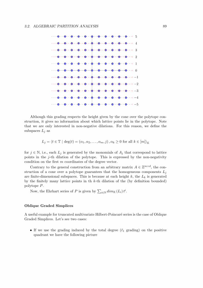
3.2. ALGEBRAIC PARTITION ANALYSIS 89
5
4
3
2
1
0
−1
−2
−3
−4
−5
Although this grading respects the height given by the cone over the polytope con-struction, it gives no information about which lattice points lie in the polytope. Notethat we are only interested in non-negative dilations. For this reason, we define thesubspaces 𝐿𝑗 as
𝐿𝑗 = ⟨𝑡 ∈ T | deg(𝑡) = (𝛼1, 𝛼2, . . . , 𝛼𝑚, 𝑗) , 𝛼𝑘 ≥ 0 for all 𝑘 ∈ [𝑚]⟩K
for 𝑗 ∈ N, i.e., each 𝐿𝑗 is generated by the monomials of 𝐴𝑗 that correspond to latticepoints in the 𝑗-th dilation of the polytope. This is expressed by the non-negativitycondition on the first 𝑚 coordinates of the degree vector.
Contrary to the general construction from an arbitrary matrix 𝐴 ∈ Z𝑚×𝑑, the con-struction of a cone over a polytope guarantees that the homogeneous components 𝐿𝑗
are finite-dimensional subspaces. This is because at each height 𝑘, the 𝐿𝑘 is generatedby the finitely many lattice points in th 𝑘-th dilation of the (by definition bounded)polytope 𝑃 .
Now, the Ehrhart series of 𝑃 is given by∑
𝑖∈N 𝑑𝑖𝑚K (𝐿𝑖) 𝑡𝑖.
Oblique Graded Simplices
A useful example for truncated multivariate Hilbert-Poincare series is the case of ObliqueGraded Simplices. Let’s see two cases:
∙ If we use the grading induced by the total degree (ℓ1 grading) on the positivequadrant we have the following picture

90 CHAPTER 3. PARTITION ANALYSIS
and the corresponding truncated multivariate Hilbert-Poincare series is the gener-ating function for the lattice points in the positive quadrant graded by the givengrading. Note that if 𝑉 is the grading constructed as above, then
ℎ′𝑖(𝑧) = [𝑡𝑖]𝑡ℋ𝒫𝑉 (𝑧, 𝑡)
are the usual complete homogeneous symmetric polynomial of degree 𝑖.
∙ If we use the degree function given by degree(𝑥, 𝑦) = 𝑥+ 2𝑦 the picture is
and thenℎ′𝑖(𝑧) = [𝑡𝑖]𝑡ℋ𝒫𝑉 (𝑧, 𝑡)
are the oblique complete homogeneous polynomials ℎ𝑖(𝑧; 1, 2).
In [5], the authors introduce ℎ𝑖(𝑧1, 𝑧2, . . . , 𝑧𝑛; 𝜁1, 𝜁2, . . . , 𝜁𝑛) for 𝜁𝑖 ∈ N, “a variant ofthe symmetric functions”, given by their generating function
∞∑𝑖=0
ℎ𝑖(𝑧1, 𝑧2, . . . , 𝑧𝑛; 𝜁1, 𝜁2, . . . , 𝜁𝑛)𝑡𝑖 =
1
(1− 𝑧1𝑡𝜁1)(1− 𝑧2𝑡𝜁2) · · · (1− 𝑧𝑛𝑡𝜁𝑛).

Chapter 4
Partition Analysis via PolyhedralGeometry
The main idea behind all implementations of the Ω≥ operator is to obtain a partial-fraction decomposition of the crude generating function and exploit the linearity of theΩ≥ operator. In particular, we want a partial-fraction decomposition such that in thedenominator of each fraction appear either only non-negative or only non-positive powersof 𝜆’s. Given such a partial-fraction decomposition, we can be sure that in the seriesexpansions of the crude generating function with respect to the 𝜆’s, the fractions withonly non-positive powers of 𝜆 cannot contribute terms with positive 𝜆 exponents. Inother words, we should only keep the fractions that have non-negative powers of 𝜆 andthe fractions that are 𝜆-free. There are different ways to compute such a partial-fractiondecomposition, like Elliott’s algorithm [24] and Omega2 [5].
In this chapter, we present an algorithmic geometric approach. The main goal ofthe method presented here is to compute a cone decomposition of the Ω-polyhedron.Instead of going directly for the rational generating function of the lattice points in theΩ-polyhedron, we first compute a set of simplicial cones that sum up to the desiredpolyhedron. This step is done by using only rational linear algebra. In order to obtainthe rational generating function, one can either use Barvinok’s algorithm or explicitformulas. Some more custom-tailored tools will appear in [19]. Here we restrict tocomputing a set of “symbolic cones”, i.e., instead of using the actual generating functionwe say “the cone generated by 𝑎1, 𝑎2, . . . , 𝑎𝑘 with apex 𝑞”. This work is part of [19].
Recall the definitions of the rational form of the crude generating function
𝜌Ω𝐴,𝑏(𝑧;𝜆) = Ω≥𝜆−𝑏∏𝑚
𝑖=1(1− 𝑧𝑖𝜆𝐴𝑖)
and of the formal Laurent series form
ΦΩ𝐴,𝑏(𝑧;𝜆) = Ω≥
∑𝑥1,...,𝑥𝑑∈N
𝜆𝐴𝑥−𝑏𝑧𝑥11 . . . 𝑧𝑥𝑑
𝑑 ,
91

92 CHAPTER 4. PARTITION ANALYSIS VIA POLYHEDRAL GEOMETRY
as well as that of the formal Laurent series form of the 𝜆-generating function
Φ𝜆𝐴,𝑏(𝑧) =
∑𝑥1,...,𝑥𝑑∈N
𝜆𝐴𝑥−𝑏𝑧𝑥11 . . . 𝑧𝑥𝑑
𝑑
and its rational form
𝜌𝜆𝐴,𝑏(𝑧) =𝜆−𝑏∏𝑛
𝑖=1(1− 𝑧𝑖𝜆𝐴𝑖).
We will denote by𝐴 the matrix with𝐴1, 𝐴2, . . . , 𝐴𝑛 as columns. We note that 𝜌Π𝐶(𝑧) and
ΦΠ𝐶(𝑧), where Π𝐶 denotes the fundamental parallelepiped of the cone 𝐶, are identical
since the fundamental parallelepiped is finite and both objects collapse to a Laurentpolynomial.
4.1 Eliminating a single 𝜆
Elimination of a single 𝜆 amounts to the solution of a single linear Diophantine inequality.All known implementations of the Ω≥ operator are based on the recursive eliminationof 𝜆’s for the solution of linear Diophantine systems. In order to employ polyhedralgeometry, we need to translate the problem to a problem about cones. Recall thedefinitions of the 𝜆-cone and the Ω-polyhedron:
𝒞𝜆,Z (𝐴) = 𝒞R ((𝑒1 : 𝐴1), (𝑒2 : 𝐴2), . . . , (𝑒𝑑 : 𝐴𝑚))
𝒫Ω≥,Rb (𝐴) = {x ∈ R𝑑
+ : 𝐴x ≥ b}Let 𝐻𝑏 = {(𝑥1, . . . , 𝑥𝑑, 𝑥𝑑+1) : 𝑏 ≤ 𝑥𝑑+1} be the set of vectors with last componentgreater or equal to 𝑏. Since we have one 𝜆, the 𝐴𝑖 is an integer denoted by 𝑎𝑖.
Computing Ω≥𝜆−𝑏
(1−𝑧1𝜆𝑎1 )·...·(1−𝑧𝑑𝜆𝑎𝑑 ) amounts to computing the generating function
𝜌𝜋(𝐶∩𝐻𝑏)(𝑧1, . . . , 𝑧𝑑), where 𝜋 denotes projection with respect to the last coordinate, as
follows:
1. Compute a vertex description of the vertex cones 𝒦𝑣 at the vertices of 𝐶 ∩𝐻𝑏.
2. Compute the generating functions 𝜌𝒦𝑣(𝑧1, 𝑧2, . . . , 𝑧𝑑+1), either using Barvinok’s
algorithm [12] or by explicit formulas using modular arithmetic (similar to theexpressions in [5]).
3. Substitute 𝑧𝑑+1 ↦→ 1 to obtain 𝜆-free generating functions (projection of the poly-hedron).
4. Sum all the projected generating functions for the tangent cones. By Brion’stheorem [12], this yields the desired generating function Ω≥
𝜆−𝑏
(1−𝑧1𝜆𝑎1 )·...·(1−𝑧𝑑𝜆𝑎𝑑 ) .
Let 𝑃 be the polyhedron 𝐶 ∩𝐻𝑏. We need to compute the vertices and vertex conesof 𝑃 . We note that any polyhedron can be written as the Minkowski sum of a cone anda polytope. In our case
𝑃 = conv(0, 𝑢𝑖 : 𝑖 ∈ {1, . . . , ℓ}) + 𝒞R (𝑤𝑖,𝑗 : 𝑖 ∈ {1, . . . , ℓ}, 𝑗 ∈ {ℓ+ 1, . . . , 𝑑})
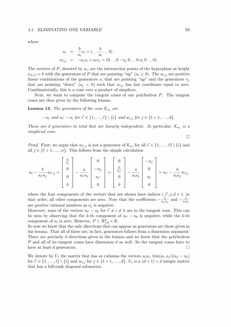
4.1. ELIMINATING ONE VARIABLE 93
where
𝑢𝑖 =𝑏
𝑎𝑖𝑣𝑖 = (. . .
𝑏
𝑎𝑖. . . 𝑏)
𝑤𝑖,𝑗 = −𝑎𝑗𝑣𝑖 + 𝑎𝑖𝑣𝑗 = (0 . . . 0 −𝑎𝑗 0 . . . 0 𝑎𝑖 0 . . . 0).
The vertices of 𝑃 , denoted by 𝑢𝑖, are the intersection points of the hyperplane at height𝑥𝑑+1 = 𝑏 with the generators of 𝑃 that are pointing “up” (𝑎𝑖 ≥ 0). The 𝑤𝑖,𝑗 are positivelinear combinations of the generators 𝑣𝑖 that are pointing “up” and the generators 𝑣𝑗that are pointing “down” (𝑎𝑗 < 0) such that 𝑤𝑖,𝑗 has last coordinate equal to zero.Combinatorially, this is a cone over a product of simplices.
Next, we want to compute the tangent cones of our polyhedron 𝑃 . The tangentcones are then given by the following lemma.
Lemma 13. The generators of the cone 𝒦𝑢𝑖 are
−𝑢𝑖 and 𝑢𝑖′ − 𝑢𝑖 for 𝑖′ ∈ {1, . . . , ℓ} ∖ {𝑖} and 𝑤𝑖,𝑗 for 𝑗 ∈ {ℓ+ 1, . . . , 𝑑}.
These are 𝑑 generators in total that are linearly independent. In particular, 𝒦𝑢𝑖 is asimplicial cone.
�
Proof. First, we argue that 𝑤𝑖′,𝑗 is not a generator of 𝒦𝑢𝑖 for all 𝑖′ ∈ {1, . . . , ℓ} ∖ {𝑖} and
all 𝑗 ∈ {ℓ+ 1, . . . , 𝑛}. This follows from the simple calculation
𝑢𝑖 −𝑏
𝑎𝑖′𝑎𝑗𝑤𝑖′,𝑗 =
⎡⎢⎢⎢⎢⎢⎢⎣𝑏𝑎𝑖
0
0
𝑏
⎤⎥⎥⎥⎥⎥⎥⎦−𝑎
𝑎𝑖′𝑎𝑗
⎡⎢⎢⎢⎢⎢⎢⎣0
−𝑎𝑗
𝑎𝑖′
0
⎤⎥⎥⎥⎥⎥⎥⎦ =
⎡⎢⎢⎢⎢⎢⎢⎣0
𝑏𝑎𝑖′
0
𝑏
⎤⎥⎥⎥⎥⎥⎥⎦−𝑎
𝑎𝑖𝑎𝑗
⎡⎢⎢⎢⎢⎢⎢⎣−𝑎𝑗
0
𝑎𝑖
0
⎤⎥⎥⎥⎥⎥⎥⎦ = 𝑢𝑖′ −𝑏
𝑎𝑖𝑎𝑗𝑤𝑖,𝑗
where the four components of the vectors that are shown have indices 𝑖, 𝑖′, 𝑗, 𝑑 + 1, inthat order, all other components are zero. Note that the coefficients − 𝑏
𝑎𝑖′𝑎𝑗and − 𝑏
𝑎𝑖𝑎𝑗are positive rational numbers as 𝑎𝑗 is negative.Moreover, none of the vectors 𝑢𝑖′ − 𝑢𝑘 for 𝑖′ = 𝑖 = 𝑘 are in the tangent cone. This canbe seen by observing that the 𝑘-th component of 𝑢𝑖′ − 𝑢𝑘 is negative, while the 𝑘-thcomponent of 𝑢𝑖 is zero. However, 𝑃 ⊂ R𝑑
≥0 × R.So now we know that the only directions that can appear as generators are those given inthe lemma. That all of these are, in fact, generators follows from a dimension argument:There are precisely 𝑑 directions given in the lemma and we know that the polyhedron𝑃 and all of its tangent cones have dimension 𝑑 as well. So the tangent cones have tohave at least 𝑑 generators.
We denote by 𝑈𝑖 the matrix that has as columns the vectors 𝑎𝑖𝑢𝑖, lcm(𝑎𝑖, 𝑎𝑖′)(𝑢𝑖′ − 𝑢𝑖)for 𝑖′ ∈ {1, . . . , ℓ} ∖ {𝑖} and 𝑤𝑖,𝑗 for 𝑗 ∈ {ℓ+ 1, . . . , 𝑑}. 𝑈𝑖 is a (𝑑+ 1)× 𝑑 integer matrixthat has a full-rank diagonal submatrix.

94 CHAPTER 4. PARTITION ANALYSIS VIA POLYHEDRAL GEOMETRY
By Brion’s theorem, the generating function for 𝜋(𝑃∩𝐻𝑏) is the sum for all 𝑖 of the gener-ating function of the cone generated by the columns of 𝑈𝑖 and equal to 𝜌𝐶(𝑧1, 𝑧2, . . . , 𝑧𝑑).We can now present the algorithm:
Algorithm 2 Elimination of a single 𝜆
Require: 𝑏 ∈ Z and 𝐴 ∈ Z𝑑 such that 𝑎1, 𝑎2, . . . , 𝑎ℓ > 𝑏 and 𝑎ℓ+1, 𝑎ℓ+2, . . . , 𝑎𝑑 < 𝑏
1: 𝐼+ ← {1, . . . , ℓ}2: 𝐼+ ← {ℓ+ 1, . . . , 𝑑}3: for 𝑖 ∈ 𝐼+ do4: 𝑣𝑖 ← (𝑒𝑖 : 𝑎𝑖)
5: 𝑈 ← {(. . . 𝑏𝑎𝑖. . . 𝑏)} for 𝑖 ∈ 𝐼+
6: for 𝑖 ∈ 𝐼+ do7: for 𝑗 ∈ 𝐼− do8: 𝑤𝑖,𝑗 ← −𝑎𝑗𝑒𝑖 + 𝑎𝑖𝑒𝑗
9: for 𝑖 ∈ 𝐼+ do10: 𝑈𝑖 ← {−𝑢𝑖, 𝑢𝑖′ − 𝑢𝑖, 𝑤𝑖,𝑗 : 𝑖
′ ∈ 𝐼+ ∖ {𝑖}, 𝑗 ∈ 𝐼−}11: 𝑇𝑖 ← a triangulation of the vertex cone 𝒞R (𝑈𝑖)
12: 𝜌𝒞R(𝑈𝑖)(𝑧1, 𝑧2, . . . , 𝑧𝑑+1) ←
∑𝑠∈𝑇𝑖
𝜌𝑠(𝑧1, 𝑧2, . . . , 𝑧𝑑+1)
13: 𝜌(𝑧1, 𝑧2, . . . , 𝑧𝑑+1) ←∑𝑖∈𝐼+
𝜌𝑈𝑣(𝑧1, 𝑧2, . . . , 𝑧𝑑+1)
14: return 𝜌(𝑧1, 𝑧2, . . . , 𝑧𝑑, 1)
To illustrate the algorithm we present an example.
Example 12. Given an inequality 2𝑥1 + 3𝑥2 − 5𝑥3 ≥ 4, we want to compute
Ω≥𝜆−4
(1− 𝑧1𝜆2)(1− 𝑧2𝜆3)(1− 𝑧3𝜆−5).
We first compute the generators of 𝒞𝜆,Z (𝐴):
𝑣1 = (1, 0, 0, 2), 𝑣2 = (0, 1, 0, 3), 𝑣3 = (0, 0, 1,−5)
and construct the matrix 𝑉 :
𝑉 =
⎡⎢⎢⎢⎢⎢⎢⎣1 0 0
0 1 0
0 0 1
2 3 −5
⎤⎥⎥⎥⎥⎥⎥⎦ .
We want to compute the generating function of the intersection of 𝒞𝜆,Z (𝐴) and 𝐻4 ={(𝑥1, 𝑥2, 𝑥3, 𝑥4) ∈ R4 : 𝑥4 ≥ 4}.
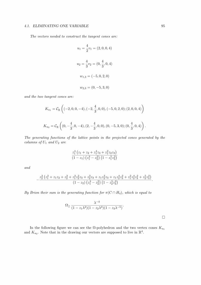
4.1. ELIMINATING ONE VARIABLE 95
The vectors needed to construct the tangent cones are:
𝑢1 =4
2𝑣1 = (2, 0, 0, 4)
𝑢2 =4
3𝑣2 = (0,
4
3, 0, 4)
𝑤1,3 = (−5, 0, 2, 0)
𝑤2,3 = (0,−5, 3, 0)
and the two tangent cones are:
𝐾𝑢1 = 𝒞R((−2, 0, 0,−4), (−2, 4
3, 0, 0), (−5, 0, 2, 0); (2, 0, 0, 4)
)
𝐾𝑢2 = 𝒞R((0,−4
3, 0,−4), (2,−4
3, 0, 0), (0,−5, 3, 0); (0, 4
3, 0, 4)
).
The generating functions of the lattice points in the projected cones generated by thecolumns of 𝑈1 and 𝑈2 are
𝑧41(𝑧1 + 𝑧2 + 𝑧41𝑧3 + 𝑧21𝑧2𝑧3
)(1− 𝑧1)
(𝑧31 − 𝑧22
) (1− 𝑧51𝑧
23
)and
−𝑧22(𝑧21 + 𝑧1𝑧2 + 𝑧22 + 𝑧21𝑧
22𝑧3 + 𝑧32𝑧3 + 𝑧1𝑧
32𝑧3 + 𝑧1𝑧
42𝑧
23 + 𝑧21𝑧
42𝑧
23 + 𝑧52𝑧
23
)(1− 𝑧2)
(𝑧31 − 𝑧22
) (1− 𝑧52𝑧
33
) .
By Brion their sum is the generating function for 𝜋(𝐶 ∩𝐻4), which is equal to
Ω≥𝜆−4
(1− 𝑧1𝜆2)(1− 𝑧2𝜆3)(1− 𝑧3𝜆−5).
�
In the following figure we can see the Ω-polyhedron and the two vertex cones 𝐾𝑢1
and 𝐾𝑢2 . Note that in the drawing our vectors are supposed to live in R4.

96 CHAPTER 4. PARTITION ANALYSIS VIA POLYHEDRAL GEOMETRY
The two vertex cones. Elimination of a single 𝜆.
The discussion above and Lemma 13 give us the following theorem that summarizesthe algorithm for the elimination of one 𝜆. Note that instead of taking the halfspace𝐻𝑏, we translate the cone by −𝑏 and use the positive halfspace with respect to the 𝜆coordinate denoted by 𝐻𝜆. The subscript does not mean the offset but denotes thecoordinate.
Theorem 2. Let 𝑎1, . . . , 𝑎𝑘 ∈ Q𝑛 be linearly independent vectors, let 𝐴 ∈ Q𝑛×𝑘 denotethe matrix with the 𝑎𝑖 as columns, let 𝑏 ∈ Q𝑛, and let 𝐼 ⊂ [𝑘]. Then 𝒞𝐼R (𝐴; 𝑏) isan inhomogeneous simplicial cone. Assume that the affine hull of 𝒞𝐼R (𝐴; 𝑏) contains
integer points. Let 𝜆 ∈ [𝑛] and define 𝐻≥𝜆 = {𝑥 ∈ R𝑛 | 𝑥𝜆 ≥ 0} to be the non-negative
half-space with respect to the coordinate 𝜆. Let ℐ+, ℐ−, ℐ0 denote the sets of indices𝑖 ∈ [𝑘] with 𝑎𝑖𝜆 > 0, 𝑎𝑖𝜆 < 0 and 𝑎𝑖𝜆 = 0, respectively. Let 𝑃 denote the polyhedron𝑃 = 𝐻≥
𝜆 ∩ (𝒞𝐼R (𝐴; 𝑏)). Under these assumptions, the following hold.If 𝑏𝜆 < 0, then:
1. The vertices of 𝑃 are
𝑣𝑖 = 𝑏− 𝑏𝜆𝑎𝑖𝜆
𝑎𝑖 for 𝑖 ∈ ℐ+,
2. For every 𝑖 ∈ ℐ+, the extreme rays of the tangent cone of 𝑃 at 𝑣𝑖 are generated bythe vectors 𝑔1, . . . , 𝑔𝑘 defined by
𝑔𝑖 = 𝑎𝑖
𝑔𝑖′ = 𝑎𝑖′ − 𝑎𝑖 for all 𝑖′ ∈ ℐ+ ∖ {𝑖}
𝑔𝑗 =1
𝑎𝑗𝜆𝑎𝑗 −
1
𝑎𝑖𝜆𝑎𝑖 for all 𝑗 ∈ ℐ−
𝑔𝑙 = 𝑎𝑙 for all 𝑙 ∈ ℐ0.
The vectors 𝑔𝑖 are linearly independent whence the tangent cone at 𝑣𝑖 is simplicial.Let 𝐺𝑖 denote the matrix with these vectors as columns.

4.1. ELIMINATING ONE VARIABLE 97
3. The half-open tangent cone of 𝑃 at 𝑣𝑖 is
𝒦𝑣𝑖 = 𝑣𝑖 + 𝒞𝐼∖𝑖R (𝐺𝑖; 0) .
In particular, the tangent cone is “open in direction 𝑔𝑠 if and only if the cone westarted out with is open in direction 𝑎𝑠” for all 𝑠 = 𝑖. It is closed in direction 𝑖,because we intersect with a closed half-space.
4. For any vertex 𝑣𝑖, let 𝐽𝑖 denote the set of indices 𝑠 ∈ [𝑘] where 𝑠 ∈ 𝐽𝑖 if and onlyif the first non-zero component of 𝑔𝑠 is negative (i.e. if 𝑔𝑠 is backward). Let 𝐺′
𝑖
denote the matrix obtained from 𝐺𝑖 by multiplying all columns with an index in 𝐽𝑖by −1. (Now all columns of 𝐺𝑖 are forward.) Then
Φ(𝒞𝐼
R(𝐴;𝑏))∩𝐻≥𝜆
=∑𝑖∈ℐ+
(−1)|𝐽𝑖|Φ𝒞R()𝐼∖𝑖Δ 𝐽𝑖 (𝐺′
𝑖)+𝑣𝑖
where Δ denotes the symmetric difference. The same identity also holds on thelevel of rational functions.
5. Let 𝜋 : R𝑛 → R𝑛−1 denote the projection that forgets the 𝜆-th coordinate. Ifaff(𝐶) ∩ 𝐿 = 0 for some linear subspace 𝐿 that contains ker(𝜋), then
Ω𝜆Φ𝒞𝐼R(𝐴;𝑏)
=∑𝑖∈ℐ+
(−1)|𝐽𝑖|Φ𝒞𝐼∖𝑖Δ 𝐽𝑖R (��𝑖;𝑣𝑖)
.
where ��𝑖 denotes the matrix obtained from 𝐺′𝑖 by deleting the 𝜆th row. Moreover,
all the cones 𝐶𝑖 = 𝒞𝐼∖𝑖Δ 𝐽𝑖R
(��𝑖; 𝑣𝑖
)have the property that aff(𝐶𝑖) ∩ 𝜋(𝐿) = 0.
�
We note that for the case when 𝑏𝜆 > 0, the theorem is completely analogous and theonly difference is that the apex of the cone is a vertex of the polyhedron. Each othervertex is visible from the apex, thus an extra ray is added in all vertex cones (from eachvertex to the apex of the cone). If 𝑏𝜆 = 0, then not all vertex cones are simplicial. Thuswe employ a deformation argument, presented by Fu Liu in [29] , and reduce the caseto the case 𝑏𝜆 < 0.
The following lemma says that after we project we can repeat the same procedure,thus allowing for recursive elimination of 𝜆s in order to solve systems of inequalities.
Lemma 14. Assume ker(𝜋) ⊂ 𝐿. If 𝐽 ∩ 𝐿 = 0, then 𝜋(𝐽) ∩ 𝜋(𝐿) = 0. �
Proof. Let 𝑣 ∈ 𝜋(𝐽)∩ 𝜋(𝑙). Then there exist 𝑗 ∈ 𝐽 and 𝑙 ∈ 𝐿 such that 𝑣 = 𝜋(𝑗) = 𝜋(𝑙).Because 𝜋 is linear, we have that 𝑗 − 𝑙 ∈ ker(𝜋) ⊂ 𝐿. Therefore 𝑗 = 𝑗 − 𝑙+ 𝑙 ∈ 𝐿 and so𝑗 ∈ 𝐽 ∩ 𝐿 which means by assumption 𝑗 = 0. But then 𝑣 = 𝜋(𝑗) = 0.
98 CHAPTER 4. PARTITION ANALYSIS VIA POLYHEDRAL GEOMETRY
4.2 Eliminating multiple 𝜆
Using the algorithm for single 𝜆 elimination recursively (due to Lemma 14, we essentiallycompute triangulations of the dual vertex cones and their generating functions. Thisis an interesting fact which comes directly from the particular choice of geometry thatpartition analysis makes. Nevertheless, recursive elimination may not always be themost desirable strategy, as it is well known that the choice of the elimination ordermay considerably alter the running time in the traditional partition analysis algorithms(intermediate expressions swell).
In order to eliminate multiple 𝜆 we need to follow the same procedure, but now thedimension of the 𝜆-cone is more than one lower than the ambient space, since we havemore than one 𝜆. This makes the computation of explicit expressions for the verticesand the vertex cones considerably harder. In what follows we give a description of howthis could be done algorithmically.
Given 𝐴 ∈ Z𝑚×𝑑 and 𝑏 ∈ Z𝑚 for 𝑚 ≥ 1, we define the vectors 𝑣𝑖 = (𝑒𝑖 : 𝐴𝑖) ∈ R𝑑+𝑚
where 𝐴𝑖 denotes the 𝑖-th column of 𝐴 and 𝑒𝑖 the 𝑖-th standard unit vector in R𝑑. Let 𝑉denote the matrix with the 𝑣𝑖 as columns. Then 𝑉 is a vertex description of the 𝜆-cone
𝐶 = 𝒞𝜆,ZR (𝐴) = 𝒞R (𝑉 ) .
The Ω-polyhedron we want to compute is now
𝑃 = 𝒞R (𝑉 ) ∩{(𝑧, 𝜆) ∈ R𝑑+𝑚
𝜆𝑖 ≥ 𝑏𝑖 for all 𝑖 = 1, . . . ,𝑚
}.
Note that this definition of 𝑃 is neither a vertex-description nor a hyperplane-description.We need to compute the vertices and the tangent cones at the vertices of our polyhedronand we will follow a standard method for that [38].It is straightforward to give a hyperplane-description of 𝐶. Note that 𝐶 is a simplicial𝑑-dimensional cone. Its facets are spanned by all combinations of 𝑑−1 generators of thecone.
Lemma 15.
span(𝐶) =
⎧⎨⎩⎛⎝𝑥
ℓ
⎞⎠ ∈ R𝑑+𝑚
(𝐴 −𝐼
)⎛⎝𝑥
ℓ
⎞⎠ = 0
⎫⎬⎭ .
�
Proof. There exist 𝛼𝑖 such that 𝑥 =∑
𝑖 𝛼𝑖𝑣𝑖 if and only if there exist 𝛼𝑖 such that𝑥𝑖 = 𝛼𝑖 for 𝑖 = 1, . . . , 𝑑 and ℓ𝑗 =
∑𝑖 𝛼𝑖𝜆𝑗,𝑖 for 𝑗 = 1, . . . ,𝑚. Such 𝛼𝑖 exist if and only if
ℓ𝑗 =∑𝑑
𝑖=1 𝑥𝑖𝜆𝑗,𝑖 for all 𝑗 = 1, . . . ,𝑚.
Given the linear span of 𝐶, we can write down a hyperplane description of 𝑃 .
Lemma 16.
𝑃 =
⎧⎨⎩⎛⎝𝑥
ℓ
⎞⎠ ∈ R𝑑+𝑚
⎛⎝𝑥
ℓ
⎞⎠ ≥⎛⎝0
𝑏
⎞⎠ and(𝐴 −𝐼
)⎛⎝𝑥
ℓ
⎞⎠ = 0
⎫⎬⎭ .

4.2. ELIMINATING MULTIPLE VARIABLES 99
�
Proof. From the proof of the previous lemma, we see that 𝑥 =∑
𝑖 𝛼𝑖𝑣𝑖 for 𝛼𝑖 ≥ 0 if andonly if 𝑥𝑖 ≥ 0 for 𝑖 = 1, . . . , 𝑑 and
(𝐴 −𝐼
)⎛⎝𝑥
ℓ
⎞⎠ = 0.
So
𝐶 =
⎧⎨⎩⎛⎝𝑥
ℓ
⎞⎠ ∈ R𝑑+𝑚
𝑥 ≥ 0 and
(𝐴 −𝐼
)⎛⎝𝑥
ℓ
⎞⎠ = 0
⎫⎬⎭whence the theorem follows from the definition of 𝑃 .
Having the H-description of the Ω-polyhedron, what we need to do first is computeits vertices. This is done by considering all the full-rank square subsystems of the system⎛⎝𝑥
ℓ
⎞⎠ =
⎛⎝0
𝑏
⎞⎠(𝐴 −𝐼
)⎛⎝𝑥
ℓ
⎞⎠ = 0.
Each system has (at most) one rational solution. If the solution satisfies the full sys-tem (the point lies in the polyhedron), then that solution is a vertex of the Ω-polyhedron.
Unfortunately, unlike the single 𝜆 case, explicit formulas are no more easy to obtainfor the vertex cones. This is due to the fact that there are many combinations ofpositive/negative entries in the inhomogeneous part. Thus, one can not simply labelgenerators as pointing up or down, since the same generator may be pointing up withrespect to one 𝜆 coordinate and down with respect to another.
We resort to the use of standard tools from polyhedral geometry.
∙ Compute the vertex cones, which is possible since we have both an H-descriptionand a V-description of the polyhedron.
∙ Triangulate if needed. The nice simplicial structure of the vertex cones is no longerguaranteed.
∙ Use Brion’s theorem and Barvinok’s algorithm in order to compute the desiredrational generating function.
This method is algorithmic, but no closed formulas for the vertices and the vertexcones are provided. Nevertheless, while its performance will be poorer than that oftraditional recursive elimination algorithms in general, it is expected to perform betterthan traditional algorithms on problems that show intermediate expression swell. This

100 CHAPTER 4. PARTITION ANALYSIS VIA POLYHEDRAL GEOMETRY
latter case is very often met in combinatorial problems, which have a nice 1 generatingfunction due to the structure of the problem, but the intermediate expressions do notsee the overall structure. One could say that this is a difference between local or globalknowledge about the problem structure.
1this usually means that a lot of cancellations occur in the rational function.

4.3. IMPROVEMENTS BASED ON GEOMETRY 101
4.3 Improvements based on geometry
4.3.1 Lattice Points in Fundamental Parallelepipeds
In this section we develop a closed formula for the generating function of the set of latticepoints in the fundamental parallelepiped of a simplicial cone. We will first illustrate thebasic idea for finding this lattice point set using an example.
Motivating Example
Let 𝐽 ⊂ R𝑛 be a lattice and 𝐿 a sublattice with basis 𝑎1, . . . , 𝑎𝑘 ∈ 𝐽 . Our goal is tocome up with a closed formula (or simply a way of enumerating) the 𝐽-lattice pointsin the fundamental parallelepiped generated by the 𝑎𝑖, i.e., we want to come up with agenerating function for the set Π(𝐴) where 𝐴 is the 𝑛× 𝑘-matrix with the vectors 𝑎𝑖 ascolumns.
As an example we will take 𝐽 = Z2 and
𝐴 =
⎡⎣ 2 6
−2 2
⎤⎦ .
The fundamental parallelepiped Π(𝐴) and the lattice points contained therein are illus-trated in Figure 4.1.
Figure 4.1: The lattice points in the fundamental parallelepiped Π(𝐴).
If Π(𝐴) were a rectangle, or, more precisely, if 𝐴 were a diagonal matrix, then𝐽 ∩Π(𝐴) would be particularly easy to describe. For example if 𝐴 is an 𝑛× 𝑛 diagonalmatrix with diagonal entries 𝑙1, . . . , 𝑙𝑛, then we have
Π(𝐴) = [0, 𝑙1)× · · · × [0, 𝑙𝑛)
Z𝑛 ∩Π(𝐴) = {0, . . . , 𝑙1 − 1} × · · · × {0, . . . , 𝑙𝑛 − 1}
ΦΠ(𝐴)(𝑧) =1− 𝑧𝑙111− 𝑧1
· . . . · 1− 𝑧𝑙𝑛𝑛1− 𝑧𝑛
.
How can we make use of this simple observation about rectangles to handle generalmatrices 𝐴 such as our example above? One idea is to transform 𝐴 into a diagonal
102 CHAPTER 4. PARTITION ANALYSIS VIA POLYHEDRAL GEOMETRY
matrix and control the corresponding changes to Π(𝐴). To implement this approach wecan use the Smith normal form of a matrix.
Theorem 4.1(Smith normal form) Let 𝐴 be a non-zero 𝑛×𝑘 integer matrix. Then there exist matrices𝑈 ∈ Z𝑛×𝑛, 𝑆 ∈ Z𝑛× 𝑘, 𝑉 ∈ Z𝑘×𝑘 such that 𝐴 = 𝑈𝑆𝑉 , the matrices 𝑈 and 𝑉 areinvertible over the integers (i.e., they are lattice transformations), and
𝑆 =
⎡⎢⎢⎢⎢⎢⎢⎢⎢⎢⎢⎢⎢⎢⎢⎢⎢⎣
𝑠1 0 0 · · · 0
0 𝑠2 0 · · · 0
0 0. . .
...... 𝑠𝑟
0
. . .
0 0 0
⎤⎥⎥⎥⎥⎥⎥⎥⎥⎥⎥⎥⎥⎥⎥⎥⎥⎦.
where 𝑟 is the rank of 𝐴 and 𝑠𝑖|𝑠𝑖+1 and 𝐴 = 𝑈𝑆𝑉 . �
In our case this can be interpreted as follows:
∙ Intuitively, multiplying 𝐴 from the left with a lattice transform 𝑈−1 means per-forming elementary row operations on 𝐴, which corresponds to changing the basisof 𝐽 . This simply applies a change of coordinates to the lattice points in thefundamental parallelepiped.
∙ Multiplying 𝐴 from the right with a lattice transform 𝑉 −1 means performing el-ementary column operation on 𝐴, which corresponds to changing the basis of 𝐿and thus changing the fundamental parallelepiped. We will return to the questionhow to relate 𝐽 ∩Π(𝐴) and 𝐽 ∩Π(𝐴𝑉 −1) in a moment.
The result of applying both of these transformations to 𝐴 is a diagonal matrix 𝑆. Sothe Smith normal form presents a method of changing bases for both 𝐽 and 𝐿 such thatthe fundamental parallelepiped is a rectangle with respect to the new bases.
Let’s see how this plays out in our example, see Figure 4.2. We start out with 𝑒1, 𝑒2as a basis for Z2 and 𝑎1, 𝑎2 as our basis for 𝐿. Our first step is to change bases on 𝐿by replacing 𝑒1 with 𝑒′1 = 𝑒1 − 𝑒2 and keeping 𝑒′2 = 𝑒2. We then have 𝑎1 = 2𝑒′1. Thiscorresponds to the multiplication
𝑈−1𝐴 =
⎡⎣ 1 0
1 1
⎤⎦⎡⎣ 2 6
−2 2
⎤⎦ =
⎡⎣ 2 6
0 8
⎤⎦ .
As we can see, the colums of the matrix on the right hand side give the coordinates of𝑎1, 𝑎2 in terms of 𝑒′1, 𝑒
′2.

4.3. IMPROVEMENTS BASED ON GEOMETRY 103
The next step is to changes bases of 𝐿 and replace 𝑎2 with 𝑎′2 = 𝑎2−3𝑎1 and keeping𝑎′1 = 𝑎1. This corresponds to the multiplication
(𝑈−1𝐴)𝑉 −1 =
⎡⎣ 2 6
0 8
⎤⎦ .
⎡⎣ 1 −3
0 1
⎤⎦ =
⎡⎣ 2 0
0 8
⎤⎦ = 𝑆,
which gives the Smith normal form 𝑆 = 𝑈−1𝐴𝑉 −1 of 𝐴. We have now found a base𝑎′1, 𝑎
′2 of 𝐿 in which each basis vector is a multiple of the corresponding basis vector
𝑒′1, 𝑒′2. Equivalently, the matrix 𝑆 is in diagonal form, which means that with respect to
the basis 𝑒′1, 𝑒′2, the fundamental parallelepiped Π(𝑎′1, 𝑎
′2) is a rectangle:
𝐽 ∩Π(𝑎′1, 𝑎′2) =
{𝜇1𝑒
′1 + 𝜇2𝑒
′2
𝜇1 ∈ [0, 2), 𝜇2 ∈ [0, 8), 𝜇1, 𝜇2 ∈ Z
}.
Figure 4.2: By changing bases on 𝐽 and 𝐿 we can transform the parallelepiped Π(𝐴) intoa parallelepiped Π(𝑎′1, 𝑎
′2) whose generators 𝑎
′1, 𝑎
′2 are multiples of the 𝑒′1, 𝑒
′2 respectively.
The figure on the left show the bases 𝑒1, 𝑒2 of 𝐽 and 𝑎1, 𝑎2 of 𝐿 that we start out with.In the center figure, we pass from basis 𝑒1, 𝑒2 to 𝑒′1, 𝑒
′2, thereby lining up 𝑒′1 and 𝑎1. In
the right-hand figure, we pass from 𝑎1, 𝑎2 to 𝑎′1, 𝑎′2 thereby lining up 𝑒′2 and 𝑎′2. This
process corresponds to the computation of the Smith normal form of 𝐴.
We have now found a simple description of 𝐽 ∩Π(𝑎′1, 𝑎′2). How can we transform this
lattice-point set into the set 𝐽 ∩ Π(𝑎1, 𝑎2) that we are interested in? Since both 𝑎1, 𝑎2and 𝑎′1, 𝑎
′2 are bases of 𝐿, the fundamental parallelepipeds contain the same number of
lattice points. However there is no linear transformation that gives a bijection betweenthese lattice-point sets.
For any basis 𝐴 of 𝐿, the fundamental parallelepiped Π(𝐴) tiles the plane. Thismeans that for any basis 𝐴 and any point 𝑧 ∈ Z2 there is a unique 𝑦 ∈ 𝐿 such that𝑧−𝑦 ∈ Π(𝐴). If we can find a formula for this map 𝑓 : 𝑧 ↦→ 𝑧−𝑦 for any given 𝐴, we canuse this map to transform Π(𝑎′1, 𝑎
′2) into Π(𝑎1, 𝑎2). Fortunately this is straightforward.
We simply find the corrdinates 𝜆 of 𝑧 with respect to the basis 𝐴, i.e., we write 𝑧 =𝜆1𝑎1 + 𝜆2𝑎2. If we now take fractional parts, we obtain
𝑓(𝑧) = {𝜆1}𝑎1 + {𝜆2}𝑎2 ∈ Π(𝑎1, 𝑎2).

104 CHAPTER 4. PARTITION ANALYSIS VIA POLYHEDRAL GEOMETRY
Note that 𝑦 = 𝑧 − 𝑓(𝑧) = ⌊𝜆1⌋ 𝑎1 + ⌊𝜆2⌋ 𝑎2 ∈ 𝐿. Using matrices and the fractional partfunction, 𝑓 can be described simply via 𝑓 = 𝐴 ∘ frac ∘𝐴−1. This function 𝑓 is illustratedin Figure 4.3.
Figure 4.3: The lattice points in the fundamental parallelepiped Π(𝑎′1, 𝑎′2) can be
mapped into Π(𝐴) by means of the map 𝑓 = 𝐴 ∘ frac ∘𝐴−1.
On the whole, this means that we can enumerate the lattice points in the fundamentalparallelepiped we are interested in via
𝐽 ∩Π(𝑎1, 𝑎2) = 𝐴 ∘ frac ∘𝐴−1(𝐽 ∩Π(𝑎′1, 𝑎′2))
={(𝐴 ∘ frac ∘𝐴−1 ∘ 𝑈)𝜇
𝜇 ∈ Z2 ∩ ([0, 2)× [0, 8))
}where
𝐴−1 ∘ 𝑈 =
⎡⎣ 18 −3
8
18
18
⎤⎦ .
⎡⎣ 1 0
−1 1
⎤⎦ =
⎡⎣ 12 −3
8
0 18
⎤⎦ .
General Method
We now describe the method illustrated in the above example in full detail.Let 𝐽 ⊂ R𝑛 be a lattice and 𝐿 a sublattice. Most of the time, we will have 𝐽 = Z𝑛. Let
𝑎1, . . . , 𝑎𝑘 be a basis for 𝐿 and let 𝐴 denote the 𝑛×𝑘-matrix with the 𝑎𝑖 as columns. Weare then interested in describing the set of 𝐽-lattice points contained in the fundamentalparallelepiped Π(𝑎1, . . . , 𝑎𝑛) of 𝐿 with respect to the generators 𝑎1, . . . , 𝑎𝑛.
The starting point for this method is the observation that Π(𝐴) is easy to describeif the basis of 𝐿 is a multiple of a basis of 𝐽 .
Lemma 17. Let 𝐽 be a lattice with basis 𝑒1, . . . , 𝑒𝑛 and let 𝐿 be a sublattice with basis𝑎1, . . . , 𝑎𝑘 for 𝑘 ≤ 𝑛. Let 𝐼 ⊂ [𝑘]. If 𝑎𝑖 = 𝛼𝑖𝑒𝑖 for 𝑖 = 1, . . . , 𝑘 and 𝛼𝑖 ∈ Z≥1, then the

4.3. IMPROVEMENTS BASED ON GEOMETRY 105
set of 𝐽-lattice points in the fundamental parallelepiped Π𝐼(𝐴) of 𝐿 with respect to thebasis 𝐴 is
𝐽 ∩Π𝐼(𝐴) =
{𝑘∑
𝑖=1
𝜆𝑖𝑒𝑖
𝜆𝑖 ∈ Z ∀𝑖 ∈ [𝑘], 0 ≤ 𝜆𝑖 < 𝛼𝑖 ∀𝑖 ∈ 𝐼, 0 < 𝜆𝑖 ≤ 𝛼𝑖 ∀𝑖 ∈ 𝐼
}
and its generating function has the rational function representation
ΦΠ𝐼(𝐴)(𝑧) =∏𝑖∈𝐼
𝑧𝑖 ·𝑘∏
𝑖=1
1− 𝑧𝛼𝑖𝑒𝑖
1− 𝑧𝑒𝑖.
�
Proof. This follows immediately from the definition of Π𝐼(𝐴) and the fact that
𝑘∏𝑖=1
1− 𝑧𝛼𝑖𝑒𝑖
1− 𝑧𝑒𝑖=∑𝑥∈𝑆
𝑧𝑥 for 𝑆 =
{𝑘∑
𝑖=1
𝜆𝑖𝑒𝑖
𝜆𝑖 ∈ {0, . . . , 𝛼𝑖 − 1} ∀𝑖
}.
Changing the basis of 𝐿 changes the fundamental parallelepiped. However, the num-ber of lattice points in the fundamental parallelepiped remains the same. Moreover thereis a natural bijection between the lattice points in the fundamental parallelepipeds. Thisbijection is essentially given by the “fractional part” or the “division with remainder”.
To make this precise in the next lemma, we need some additional notation.For any real number 𝑥 ∈ R and 𝑒 ∈ {0, 1} we define integ𝑒(𝑥) and fract𝑒(𝑥) to be the
unique real numbers such that
𝑥 = integ𝑒(𝑥) + fract𝑒(𝑥)
and
integ𝑒(𝑥) ∈ Z, 0 ≤ fract0(𝑥) < 1, 0 < fract1(𝑥) ≤ 1.
Note that integ0 𝑥 = ⌊𝑥⌋ and fract0 𝑥 = {𝑥}. For any vector of real numbers 𝑣 ∈ R𝑘 andany set 𝐼 ⊂ [𝑘], we also write integ𝐼 𝑣 and fract𝐼 𝑣 to denote the vectors
integ𝐼(𝑣) = (integ𝑖∈𝐼(𝑣𝑖))𝑖∈[𝑘] and fract𝐼(𝑣) = (fract𝑖∈𝐼(𝑣𝑖))𝑖∈[𝑘]
where we interpret the exponent 𝑖 ∈ 𝐼 to denote 1 if 𝑖 ∈ 𝐼 and to denote 0 if 𝑖 ∈ 𝐼.In analogy to the above notation we define an extension of the mod function. Let
𝑎, 𝑏 ∈ R. We define 𝑎 mod0 𝑏 to be the unique real number 0 ≤ 𝑎 mod0 𝑏 < 𝑏 suchthat 𝑎 = 𝑘𝑏+ 𝑎 mod0 𝑏 for some 𝑘 ∈ Z. And we define 𝑎 mod1 𝑏 to be the unique realnumber 0 < 𝑎 mod1 𝑏 ≤ 𝑏 such that 𝑎 = 𝑘𝑏+ 𝑎 mod1 𝑏 for some 𝑘 ∈ Z. Again, we willwrite mod𝑖∈𝐼 to denote mod0 if 𝑖 ∈ 𝐼 and mod1 if 𝑖 ∈ 𝐼, etc. mod without exponentis understood to denote mod0 . Note that fract𝑒(𝑎𝑏 ) =
𝑎 mod𝑒 𝑏𝑏 with this notation.

106 CHAPTER 4. PARTITION ANALYSIS VIA POLYHEDRAL GEOMETRY
Lemma 18. Let 𝐽 be a lattice in R𝑛 with basis 𝑒1, . . . , 𝑒𝑛 and let 𝐿 be a sublattice. Let𝑎1, . . . , 𝑎𝑘 be a basis of 𝐿 and let 𝐴 denote the corresponding 𝑛 × 𝑘-matrix. Let 𝐴−1
denote any left inverse of 𝐴, i.e., let 𝐴−1 be a matrix with the property 𝐴−1𝑧 = 𝜆 forany 𝑧 ∈ span(𝐿) with 𝑧 =
∑𝑘𝑖=1 𝜆𝑖𝑎𝑖. Let 𝐼 ⊂ [𝑘] and let 𝑞 ∈ Q𝑛.
1. For all 𝑧 ∈ 𝐽∩(𝑞+span(𝐿)) there exists a unique lattice point 𝑦 ∈ Π𝐼(𝐴, 𝑞) such that
𝑧−𝑦 ∈ 𝐿. Let 𝑧 = 𝑞+∑𝑘
𝑖=1 𝜆𝑖𝑎𝑖 and let 𝜆 = (𝜆𝑖)𝑖=1,...,𝑘. Then 𝑦 = 𝑞+𝐴(fract𝐼(𝜆)).
2. 𝐽 ∩Π𝐼(𝐴, 𝑞) is empty if and only if 𝐽 ∩ (𝑞 + span(𝐿)) is empty.
3. Suppose 𝑝 ∈ 𝐽 ∩ (𝑞 + span(𝐿)). Let 𝑏1, . . . , 𝑏𝑘 be a second basis of 𝐿 and let 𝐵denote the corresponding 𝑛× 𝑘-matrix and let 𝐼 ′ ⊂ [𝑘]. Then
𝐽 ∩Π𝐼(𝐴, 𝑞) = 𝐴(fract𝐼(𝐴−1((𝐽 ∩Π𝐼′(𝐵))− (𝑞 − 𝑝)))) + 𝑞
and the above map induces a bijection between the sets 𝐽∩Π𝐼(𝐴, 𝑞) and 𝐽∩Π𝐼′(𝐵).
�
Note that the map 𝐴 ∘ fract𝐼 ∘𝐴−1 is not linear, as we have seen in the example.
Proof. 1. Let 𝑧 ∈ 𝐽 ∩ (𝑞+ span(𝐿)). Then there exist uniquely determined 𝜆𝑖 such that
𝑧 = 𝑞 +𝑘∑
𝑖=1
𝜆𝑖𝑎𝑖 = 𝑞 +𝑘∑
𝑖=1
integ𝑖∈𝐼(𝜆𝑖)𝑎𝑖 +𝑘∑
𝑖=1
fract𝑖∈𝐼(𝜆𝑖)𝑎𝑖.
Notice that𝑘∑
𝑖=1
integ𝑖∈𝐼(𝜆𝑖)𝑎𝑖 ∈ 𝐿 ⊂ 𝐽
and
𝑦 = 𝑞 +𝑘∑
𝑖=1
fract𝐼(𝜆𝑖)𝑎𝑖 = 𝑞 +𝐴(fract𝐼(𝜆)) ∈ Π𝐼(𝐴, 𝑞).
Moreover, 𝑦 ∈ 𝐽 because 𝑧 ∈ 𝐽 . Notice also that 𝑦 is uniquely determined as changingany coefficient by an integer amount takes us out of Π𝐼(𝐴, 𝑏).
2. By the first part of the theorem, we already know that if there exists a 𝑧 ∈𝐽 ∩ (𝑞 + span(𝐿)), then there exists a 𝑦 ∈ 𝐽 ∩ Π𝐼(𝐴, 𝑞). Conversely, if 𝑦 ∈ 𝐽 ∩ Π𝐼(𝐴, 𝑞)then 𝑦 ∈ 𝐽 ∩ (𝑞 + span(𝐿)) because Π𝐼(𝐴, 𝑞) ⊂ 𝑞 + span(𝐿).
3. Let 𝑇1 denote the translation 𝑇1(𝑥) = 𝑥− (𝑞−𝑝) and let 𝑇2 denote the translation𝑇2(𝑥) = 𝑥+ 𝑞. Using this notation we have to show that the map
𝑓 = 𝑇2 ∘𝐴 ∘ fract𝐼 ∘𝐴−1 ∘ 𝑇1
gives a bijection from 𝐽 ∩Π𝐼′(𝐵) to 𝐽 ∩Π𝐼(𝐴, 𝑞). We will proceed in five steps.Step 1: The image of 𝐽 ∩ span(𝐿) under 𝑓 is contained in 𝐽 ∩ Π𝐼(𝐴, 𝑞). Let 𝑧 ∈
𝑓(𝐽 ∩ (𝑞 + span(𝐿))). Then 𝑧 has the form 𝑧 = 𝑞 +∑𝑘
𝑖=1 fract𝐼(𝜆𝑖)𝑎𝑖 where the 𝜆𝑖 are

4.3. IMPROVEMENTS BASED ON GEOMETRY 107
such that∑𝑘
𝑖=1 𝜆𝑖𝑎𝑖 ∈ (𝐽 ∩ span𝐿) − (𝑞 − 𝑝). Therefore 𝑧 is contained in Π𝐼(𝐴, 𝑞) andit remains to show 𝑧 ∈ 𝐽 . By construction, the coefficients 𝜆𝑖 have the property
𝑘∑𝑖=1
𝜆𝑖𝑎𝑖 = −𝑘∑
𝑖=1
𝜈𝑖𝑎𝑖 +𝑘∑
𝑖=1
𝜇𝑖𝑎𝑖
where 𝑞 − 𝑝 =∑𝑘
𝑖=1 𝜈𝑖𝑎𝑖 and∑𝑘
𝑖=1 𝜇𝑖𝑎𝑖 ∈ 𝐽 . Therefore
𝑧 = 𝑞 +𝑘∑
𝑖=1
fract𝐼(𝜆𝑖)𝑎𝑖
= 𝑝+ (𝑞 − 𝑝) +𝑘∑
𝑖=1
fract𝐼(𝜆𝑖)𝑎𝑖
= 𝑝+
𝑘∑𝑖=1
𝜈𝑖𝑎𝑖 +
𝑘∑𝑖=1
fract𝐼(−𝜈𝑖 + 𝜇𝑖)𝑎𝑖
= 𝑝+𝑘∑
𝑖=1
𝜈𝑖𝑎𝑖 +𝑘∑
𝑖=1
(−𝜈𝑖 + 𝜇𝑖)𝑎𝑖 −𝑘∑
𝑖=1
integ𝐼(−𝜈𝑖 + 𝜇𝑖)𝑎𝑖
= 𝑝+𝑘∑
𝑖=1
𝜇𝑖𝑎𝑖 −𝑘∑
𝑖=1
integ𝐼(−𝜈𝑖 + 𝜇𝑖)𝑎𝑖.
Now 𝑝 and∑𝑘
𝑖=1 𝜇𝑖𝑎𝑖 are elements of 𝐽 by assumption and∑𝑘
𝑖=1 integ𝐼(−𝜈𝑖+𝜇𝑖)𝑎𝑖 is an
element of 𝐽 because the coefficients are integer and 𝐿 is a sublattice of 𝐽 . Thus 𝑧 ∈ 𝐽 .Step 2: If 𝑢, 𝑣 ∈ 𝐽 ∩ span(𝐿) and 𝑓(𝑢) = 𝑓(𝑣), then 𝑢 − 𝑣 ∈ 𝐿. Let 𝑢 =
∑𝑘𝑖=1 𝜇𝑖𝑎𝑖
and 𝑣 =∑𝑘
𝑖=1 𝜈𝑖𝑎𝑖. Let 𝑞 − 𝑝 =∑𝑘
𝑖=1 𝜅𝑖𝑎𝑖. Then 𝑓(𝑢) = 𝑓(𝑣) is equivalent to
𝑘∑𝑖=1
fract𝐼(𝜇𝑖 − 𝜅𝑖)𝑎𝑖 =𝑘∑
𝑖=1
fract𝐼(𝜈𝑖 − 𝜅𝑖)𝑎𝑖.
Then
𝑢− 𝑣 =
𝑘∑𝑖=1
(𝜇𝑖 − 𝜅𝑖)𝑎𝑖 −𝑘∑
𝑖=1
(𝜈𝑖 − 𝜅𝑖)𝑎𝑖
=𝑘∑
𝑖=1
fract𝐼(𝜇𝑖 − 𝜅𝑖)𝑎𝑖 −𝑘∑
𝑖=1
fract𝐼(𝜈𝑖 − 𝜅𝑖)𝑎𝑖 +𝑘∑
𝑖=1
integ𝐼(𝜇𝑖 − 𝜅𝑖)𝑎𝑖 −𝑘∑
𝑖=1
integ𝐼(𝜈𝑖 − 𝜅𝑖)𝑎𝑖
=𝑘∑
𝑖=1
integ𝐼(𝜇𝑖 − 𝜅𝑖)𝑎𝑖 −𝑘∑
𝑖=1
integ𝐼(𝜈𝑖 − 𝜅𝑖)𝑎𝑖
which is an integral combination of basis vectors of 𝐿 and therefore contained in 𝐿 asclaimed.

108 CHAPTER 4. PARTITION ANALYSIS VIA POLYHEDRAL GEOMETRY
Step 3: 𝑓 |𝐽∩Π𝐼′ (𝐵) is injective. As 𝐵 is a basis of 𝐿, no two distinct elements of
𝐽∩Π𝐼′(𝐵) differ by an element of 𝐿. Therefore Step 2 implies that 𝑓 |𝐽∩Π𝐼′ (𝐵) is injective.
Step 4: Both 𝐽 ∩ Π𝐼′(𝐵) and 𝐽 ∩ Π𝐼(𝐴, 𝑞) contain the same finite number of latticepoints. This follows directly from the fact that 𝐵 and 𝐴 are bases of the same lattice.
Step 5: 𝑓 |𝐽∩Π𝐼′ (𝐵) is bijective. Combining Steps 3 and 4 yields bijectivity.
The previous lemma gives us a way to keep track of Π𝐼(𝐴, 𝑞) when we change basesof 𝐿. Handling changes of bases of 𝐽 is far easier, as the next lemma tells us.
Lemma 19. If 𝑇 is a lattice transformation of the lattice 𝐽 , then
𝐽 ∩Π(𝐴; 𝑞) = 𝑇 (𝐽 ∩Π(𝑇−1𝐴;𝑇−1𝑞)).
�
Proof. This follows from 𝐽 = 𝑇𝐽 = 𝑇−1𝐽 and 𝐴𝜆 + 𝑞 = 𝑇 (𝑇−1𝐴𝜆 + 𝑇−1𝑞) for all𝜆 ∈ [0, 1)𝑘.
So far, Lemma 17 tells us that lattice-point sets in “rectangular” parallelepipeds areeasy to describe and Lemmas 18 and 19 allow us to control 𝐽 ∩Π𝐼(𝐴, 𝑞) when we changebases on 𝐿 or 𝐽 , respectively. So what is left to do is to find a way to transform anarbitrary fundamental parallelepiped Π𝐼(𝐴, 𝑞) into a “rectangular” parallelepiped usingthe transformations given in Lemmas 18 and 19. To this end we are going to use theSmith normal form as illustrated with the above example.
Lemma 20. Let 𝐽 = Z𝑛 be a lattice and 𝐿 a sublattice of 𝐽 with basis 𝑎1, . . . , 𝑎𝑘 andcorresponding 𝑛× 𝑘-matrix 𝐴. Let 𝑞 ∈ R𝑛. If 𝑞 + span(𝐿) does not contain any integerpoint, then Z𝑛 ∩Π𝐴,𝑞 is empty. Otherwise, let 𝑝 ∈ Z𝑛 ∩ span(𝐿). Then
Z𝑛 ∩Π𝐼(𝐴, 𝑞) = 𝐴 ∘ fract𝐼 ∘𝑉 −1 ∘ 𝑆−1(Z𝑘 ∩Π(𝑆)− 𝑈−1(𝑞 − 𝑝)) + 𝑞
where 𝐴 = 𝑈𝑆𝑉 is the Smith normal form of 𝐴, the numbers 𝑠1, . . . , 𝑠𝑘 are the diagonalentries of 𝑛 × 𝑘-matrix 𝑆 and 𝑆−1 is the diagonal 𝑘 × 𝑛-matrix with diagonal entries1𝑠1, . . . , 1
𝑠1. �
Note that in the above lemma
Z𝑛 ∩Π(𝑆) = Z𝑛 ∩ [0, 𝑠1)× . . .× [0, 𝑠𝑘)× {0} × . . .× {0},
is a rectangle of lattice points.
Proof. In order to be able to apply Lemma 18 we need to pick a left inverse 𝐴−1 of 𝐴.To this end we define 𝐴−1 := 𝑉 −1𝑆−1𝑈−1. As 𝑆−1𝑆 = 𝐼 is the identity, 𝐴−1 is indeeda left inverse of 𝐴 since 𝐴−1𝐴 = 𝑉 −1𝑆−1𝑈−1𝑈𝑆𝑉 = 𝐼. We then have
Z𝑛 ∩Π𝐼(𝐴, 𝑞) = 𝐴 ∘ fract𝐼 ∘𝐴−1((Z𝑛 ∩Π(𝐴𝑉 −1))− (𝑞 − 𝑝)) + 𝑞
= 𝐴 ∘ fract𝐼 ∘𝐴−1 ∘ 𝑈((Z𝑛 ∩Π(𝑈−1𝐴𝑉 −1))− 𝑈−1(𝑞 − 𝑝)) + 𝑞
= 𝐴 ∘ fract𝐼 ∘𝐴−1 ∘ 𝑈((Z𝑛 ∩Π(𝑆))− 𝑈−1(𝑞 − 𝑝)) + 𝑞
= 𝐴 ∘ fract𝐼 ∘𝑉 −1 ∘ 𝑆−1((Z𝑛 ∩Π(𝑆))− 𝑈−1(𝑞 − 𝑝)) + 𝑞

4.3. IMPROVEMENTS BASED ON GEOMETRY 109
where the first identity follows from Lemma 18 using the fact that 𝐴𝑉 −1 is a latticebasis for 𝐿, the second identity follows from Lemma 19 using the fact that 𝑈 is a latticetransformation, the third identitiy follows from 𝐴 = 𝑈𝑆𝑉 and the last identity followsfrom our choice of 𝐴−1 and 𝑆−1.
Theorem 4.2Let 𝑎1, . . . , 𝑎𝑘 ∈ Z𝑛 be linearly independent and let 𝐴 = (𝑎𝑗𝑖)𝑗∈[𝑛],𝑖∈[𝑘] be the corre-sponding matrix with Smith normal form 𝐴 = 𝑈𝑆𝑉 . Let 𝑞 ∈ R𝑛 and let 𝐼 ⊂ [𝑘]. Let𝑠1, . . . , 𝑠𝑘 denote the diagonal entries of 𝑆 and define 𝑡𝑖 =
𝑠𝑘𝑠𝑖. Note that 𝑡𝑖 ∈ Z as 𝑠𝑖|𝑠𝑖+1.
Let 𝑉 −1 = (𝑣𝑗𝑖)𝑗𝑖 where 𝑗 is the row-index and 𝑖 the column index. If 𝑝 ∈ Z𝑛 ∩ span(𝐴),then the generating function of the set of lattice points in the fundamental parallelepipedΠ𝐼(𝐴, 𝑞) is given by
Φ𝒞Z(𝐴;𝑞)(𝑥) =
𝑠1−1∑𝜆1=0
· · ·𝑠𝑘−1∑𝜆𝑘=0
𝑥
(1𝑠𝑘
∑𝑘𝑗=1 𝑎𝑙𝑗(
∑𝑘𝑖=1(𝜆𝑖−𝑤𝑖)𝑣𝑗𝑖𝑡𝑖 mod𝑖∈𝐼 𝑠𝑘)+𝑞𝑙
)𝑙=1,...,𝑛 ,
where 𝑤 = 𝑈−1(𝑞 − 𝑝). �
Proof. From Lemmas 17 and 20 we immediately get
𝑠1−1∑𝜆1=0
· · ·𝑠𝑘−1∑𝜆𝑘=0
𝑥𝐴 fract𝐼 𝑉 −1𝑆−1((𝜆1,...,𝜆𝑘,0,...,0)𝑡−𝑤)+𝑞.
We then calculate
𝑉 −1𝑆−1((𝜆1, . . . , 𝜆𝑘, 0, . . . , 0)𝑡 − 𝑤) =
(𝑘∑
𝑖=1
𝜆𝑖 − 𝑤𝑖
𝑠𝑖𝑣𝑗𝑖
)𝑗=1,...,𝑘
=1
𝑠𝑘
(𝑘∑
𝑖=1
(𝜆𝑖 − 𝑤𝑖)𝑡𝑖𝑣𝑗𝑖
)𝑗=1,...,𝑘
where we denote the entries of 𝑉 −1 by 𝑣𝑗𝑖. Recall that for 𝑒 ∈ {0, 1} we havefract𝑒(𝑎𝑏 ) =
𝑎 mod𝑒 𝑏𝑏 . With this notation we get
fract𝐼
(1
𝑠𝑘
𝑘∑𝑖=1
(𝜆𝑖 − 𝑤𝑖)𝑡𝑖𝑣𝑗𝑖
)𝑗=1,...,𝑘
=
(1
𝑠𝑘
𝑘∑𝑖=1
(𝜆𝑖 − 𝑤𝑖)𝑡𝑖𝑣𝑗𝑖 mod𝑖∈𝐼 𝑠𝑘
)𝑗=1,...,𝑘
.
Finally, we calculate
𝐴
(1
𝑠𝑘
∑𝑖
(𝜆𝑖 − 𝑤𝑖)𝑣𝑗𝑖𝑡𝑖 mod𝑖∈𝐼 𝑠𝑘
)𝑗=1,...,𝑘
+ 𝑞 =
⎛⎝ 1
𝑠𝑘
𝑘∑𝑗=1
𝑎𝑙𝑗
(𝑘∑
𝑖=1
(𝜆𝑖 − 𝑤𝑖)𝑣𝑗𝑖𝑡𝑖 mod𝑖∈𝐼 𝑠𝑘
)+ 𝑞𝑙
⎞⎠𝑙=1,...,𝑛
.

110 CHAPTER 4. PARTITION ANALYSIS VIA POLYHEDRAL GEOMETRY
4.4 Conclusions
One should note that the iterative algorithm is in the intersection of MacMahon’s ap-proach and polyhedral geometry. During the execution of the algorithm, geometricobjects such as the vertices and the vertex cones of the Ω-polyhedron, as well as a tri-angulation of the duals of the vertex cones, are computed, without use of any tool frompolyhedral geometry. Moreover, by using the intermediate step of computing cones sym-bolically, some of the cones are dropped without computing their generating functions,i.e., if all generators of a cone are pointing down and the apex lies below the intersectinghalfspace, the cone can be safely ignored.
On the other hand, the algorithm for simultaneous multiple 𝜆 elimination leansclearly towards polyhedral geometry, using exclusively tools from that area and ignoringthe recursive 𝜆 elimination, prominent in the traditional partition analysis implemen-tations. In the polyhedral geometry world, already for a decade, there exist tools, likethe algorithm of Barvinok-Woods [13] for computing Hadamard products, that can beapplied to perform simultaneous 𝜆 elimination. Nevertheless, in the partition analysisworld these tools are not yet widespread and they are not tested concerning possibleadvantages, either practical or theoretical.
A practical implementation of the algorithms and further theoretical developmentsare under preparation and will be presented in [19].

Appendix A
Proof of “Geometry of Omega2”
In what follows we assume gcd(𝛼, 𝛽) = 1 as indicated in Theorem 3.1.
Fundamental Parallelepipeds
Let Π𝜁 = Π𝐴 ∩ (Z2 × {𝜁}) and Ξ𝜁 = Π𝐵 ∩ (Z2 × {𝜁}) for 𝜁 ∈ Z. Π𝜁 (resp. Ξ𝜁) is theintersection of Π𝐴 (resp. Π𝐵 ) with the affine subspace {(𝑥, 𝑦, 𝜁) ∈ R3}.
Lemma 21. There is at most one lattice point in each fundamental parallelepiped ofthe cones 𝐴 and 𝐵 at any given height (𝑥3-value) and if there is one then its form isdetermined as follows:
∙ Π𝜁 = {(𝑥1, 𝑥2, 𝜁) ∈ Z3|𝑥1 = 𝜁−𝑥2𝛽𝛼 , 𝑥2 ∈ {0, 1, . . . , 𝛼− 1}} .
∙ Ξ𝜁 = {(𝑥1, 𝑥2, 𝜁) ∈ Z3|𝑥2 = 𝜁−𝑥1𝛼𝛽 , 𝑥1 ∈ {−𝛽 + 1,−𝛽 + 2, . . . , 0}}.
Moreover |Π𝜁 | ≤ 1 and |Ξ𝜁 | ≤ 1. �
Proof. Let (𝑥1, 𝑥2, 𝑥3) ∈ Π𝐴 ∩ Z3. Then there exist 𝑘, 𝑙 ∈ [0, 1) such that
𝑘(−𝛽, 𝛼, 0) + 𝑙(1, 0, 𝛼) = (𝑥1, 𝑥2, 𝑥3) ∈ Z3.
This translates to the system⎧⎪⎨⎪⎩𝑥1 = 𝑙 − 𝑘𝛽
𝑥2 = 𝑘𝛼
𝑥3 = 𝑙𝛼
→
⎧⎪⎨⎪⎩𝑥1 =
𝜁𝛼 − 𝑘𝛽
𝑥2 ∈ [0, 𝛼) ∩ Z𝑙 = 𝑥3
𝛼
→
⎧⎪⎨⎪⎩𝑥1 =
𝑥3−𝑥2𝛽𝛼
𝑥2 ∈ {0, 1, . . . , 𝛼− 1}𝑥3 ∈ {0, 1, . . . , 𝛼− 1}
Fix 𝑥3 = 𝜁 ∈ {0, 1, . . . , 𝛼 − 1}. Assume |Π𝜁 | > 1 and let (𝑥′1, 𝑥′2, 𝜁), (𝑥
′′1, 𝑥
′′2, 𝜁) ∈ Π𝜁 .
Then {𝛼|𝜁 − 𝑥′2𝛽
𝛼|𝜁 − 𝑥′′2𝛽→ 𝛼|𝑥′2𝛽 − 𝑥′′2𝛽 →
{𝛼|𝛽(𝑥′2 − 𝑥′′2)
gcd(𝛼, 𝛽) = 1→ 𝛼|𝑥′2 − 𝑥′′2
Since |𝑥′2 − 𝑥′′2| < 𝛼 we have a contradiction. Thus |Π𝜁 | ≤ 1.The proof for Ξ𝜁 is completely analogous.
111

112 APPENDIX A. PROOF OF “GEOMETRY OF OMEGA2”
The first summand
Our goal is to show that 𝜌𝐴 =𝑃𝛼,𝛽
(1−𝑧−𝛽1 𝑧𝛼2 )(1−𝑧1𝑧𝛼3 )
.
Proposition 4.
𝜌Π(𝐴) = 𝑃𝛼,𝛽 =
𝛼−1∑𝑖=0
𝑎𝑖𝑧𝑖3
for
𝑎𝑖 =
⎧⎨⎩𝑧𝑖𝛽
2 if 𝛽|𝑖 or 𝑖 = 0,
𝑧rmd((𝛼−1 mod 𝛽)𝑖,𝛽)−𝛽1 𝑧
rmd((𝛽−1 mod 𝛼)𝑖,𝛼)2 otherwise,
�
Proof. Since Π𝜁 = ∅ for 𝜁 ≥ 𝛼, we need to prove the following three statements
1. 𝜌Π𝜁= 1 = 𝑎0.
2. Let 𝜁 ∈ {1, 2, . . . , 𝛼− 1} such that 𝛽|𝜁. Then 𝜌Π𝜁= 𝑧
𝜆𝛽
2 𝑧𝜁3 = 𝑎𝜁𝑧𝜁3 .
3. Let 𝜁 ∈ {1, 2, . . . , 𝛼− 1} such that 𝛽 - 𝜁. Then 𝜌Π𝜁= 𝑎𝜁𝑧
𝜁3 .
Using the equations from the proof of Lemma 21 we have⎧⎪⎨⎪⎩𝑥1 = 𝑙 − 𝑘𝛽
𝑥2 = 𝑘𝛼
0 = 𝑙𝛼
𝑙=0−−→
{𝑘𝛽 ∈ Z𝑘𝛼 ∈ Z
∃𝑛∈N−−−→
{𝑘𝛽 ∈ Z𝑘 = 𝑛
𝛼
−→
{𝑛𝛽𝛼 ∈ Z𝑘 = 𝑛
𝛼
−→
{𝛼|𝑛 or 𝛼|𝛽𝑘 = 𝑛
𝛼
gcd(𝛼,𝛽)=1−−−−−−−→
{𝛼|𝑛𝑛𝛼 = 𝑘 ∈ [0, 1)
Thus 𝑘 = 0, which means 𝑥1 = 𝑥2 = 𝑥3 = 0 and 𝜌Π0= 1.
By the definition of 𝑎0 we have that 𝑎0 = 1.� of statement 1.
From Lemma 21 we know that |Π𝜁 | ≤ 1 and if equality holds the lattice point is
of the form ( 𝜁−𝑥2𝛽𝛼 , 𝑥2, 𝜁) for some 𝑥2 ∈ {0, 1, . . . , 𝛼 − 1}. We will check if the desired
exponent is actually a lattice point in Π𝜁 . Let 𝑥2 = 𝜁𝛽 . Since 𝜁 < 𝛼 we have that
𝑥2 ∈ {0, 1, . . . , 𝛼− 1}. Moreover
𝑥1 =𝜁 − 𝑥2𝛽
𝛼=
𝜁 − 𝜁𝛽𝛽
𝛼= 0 ∈ Z
which means that (0, 𝜁𝛽 , 𝜁) ∈ Π𝜁 . Thus 𝜌Π𝜁
= 𝑧𝜁𝛽
2 𝑧𝜁3 , which by definition is 𝑎𝜁𝑧𝜁3 .
� of statement 2.

113
We will proceed in two steps. First show that rmd((𝛽−1 mod 𝛼)𝜁, 𝛼) is the 𝑥2-coordinate of a lattice point in Π𝜁 and then that rmd((𝛼−1 mod 𝛽)𝜁, 𝛽) − 𝛽 is the 𝑥1-
coordinate of a lattice point in Π𝜁 . Since |Π𝜁 | ≤ 1, we have that 𝜌Π𝜁= 𝑎𝜁𝑧
𝜁3 .
∙ In order to prove that rmd((𝛽−1 mod 𝛼)𝜁, 𝛼) is the 𝑥2-coordinate of a lattice pointin Π𝜁 we have to show that
1. rmd((𝛽−1 mod 𝛼)𝜁, 𝛼) ∈ {0, 1, . . . , 𝛼− 1};
2.𝜁−(rmd((𝛽−1 mod 𝛼)𝜁,𝛼))𝛽
𝛼 ∈ Z.
Let 𝑥2 = rmd((𝛽−1 mod 𝛼)𝜁, 𝛼). By definition the remainder of division by 𝛼 is in{0, 1, . . . , 𝛼− 1}.By the definitions of remainder and modular inverse we have
𝑥2 = 𝑟𝜁 − 𝛼𝑚
for some 𝑚 ∈ Z and 𝑟 such that 𝑟𝛽 = 𝛼𝑛+ 1 for some 𝑛 ∈ Z.Then
𝑥2 = 𝑟𝜁 − 𝛼𝑚⇔ 𝛽𝑥2 = 𝛽𝑟𝜁 − 𝛼𝛽𝑚
⇔ 𝛽𝑥2 = (𝛼𝑛+ 1)𝜁 − 𝛼𝛽𝑚
⇔ 𝛽𝑥2 = 𝛼𝑛𝜁 + 𝜁 − 𝛼𝛽𝑚
⇔ 𝜁 − 𝛽𝑥2 = 𝛼(𝛽𝑚− 𝑛𝜁)
⇔ 𝜁 − 𝛽𝑥2𝛼
= 𝛽𝑚− 𝑛𝜁 ∈ Z.
∙ In order to prove that rmd((𝛼−1 mod 𝛽)𝜁, 𝛽) − 𝛽 is the 𝑥1-coordinate of a latticepoint in Π𝜁 we have to show that there exist 𝑥2 ∈ {0, 1, . . . , 𝛼 − 1} such that
rmd((𝛼−1 mod 𝛽)𝜁, 𝛽)− 𝛽 = 𝜁−𝑥2𝛽𝛼 .
Let 𝑏 = rmd((𝛼−1 mod 𝛽)𝜁, 𝛽). By definition
𝑏 = 𝑟𝜁 − 𝛽𝑚
for some 𝑚 ∈ Z and 𝑟 such that 𝛼𝑟 = 𝛽𝑛 + 1 for some 𝑛 ∈ Z. Then we want toprove that
𝑏− 𝛽 =𝜁 − 𝑥2𝛽
𝛼.
We have
𝑏− 𝛽 =𝜁 − 𝑥2𝛽
𝛼⇔ 𝑟𝜁 − 𝛽𝑚− 𝛽 =
𝜁 − 𝑥2𝛽
𝛼⇔ 𝛼𝑟𝜁 − 𝛼𝛽𝑚− 𝛼𝛽 = 𝜁 − 𝑥2𝛽
⇔ 𝛽𝑛𝜁 + 𝜁 − 𝛼𝛽𝑚− 𝛼𝛽 = 𝜁 − 𝑥2𝛽
⇔ 𝑥2 = 𝛼(𝑚+ 1)− 𝑛𝜁.

114 APPENDIX A. PROOF OF “GEOMETRY OF OMEGA2”
Thus we need to show that 𝛼(𝑚 + 1) − 𝑛𝜁 ∈ {0, 1, . . . , 𝛼 − 1}. First observe that𝛼(𝑚+ 1)− 𝑛𝜁 ∈ Z.If 𝑚 is the quotient in the division of 𝑟𝜁 by 𝛽 we have 𝑚 + 1 > 𝑟𝜁
𝛽 . In order toshow that 𝛼(𝑚+ 1)− 𝑛𝜁 > 0 we have
𝑚+ 1 >𝑟𝜁
𝛽⇒ 𝑚 >
𝑟𝜁
𝛽− 1
⇒ 𝑚 >
(𝛽𝑛+1𝛼
)𝜁
𝛽− 1
⇒ 𝑚 >𝛽𝑛𝜁 + 𝜁
𝛼𝛽− 1
⇒ 𝑚 >𝛽𝑛𝜁
𝛼𝛽− 1
⇒ 𝑚 >𝑛𝜁
𝛼− 1
⇒ 𝛼(𝑚+ 1) > 𝑛𝜁
⇒ 𝛼(𝑚+ 1)− 𝑛𝜁 > 0.
For the other direction, i.e. 𝛼(𝑚+1)−𝑛𝜁 < 𝛼 we observe that since 𝛽 - 𝜁 we have0 < 𝑏 = 𝑟𝜁 −𝑚𝛽. We know that 𝜁 < 𝛼 and
𝜁 < 𝛼𝑏⇒ 𝜁
𝛼< 𝑏
⇒ 0 < 𝑏− 𝜁
𝛼
⇒ 𝑚𝛽 < 𝑚𝛽 + 𝑏− 𝜁
𝛼
⇒ 𝑚𝛽 < 𝑟𝜁 − 𝜁
𝛼
⇒ 𝑚𝛽 <(𝑛𝛽 + 1)𝜁
𝛼− 𝜁
𝛼
⇒ 𝑚𝛽 <𝑛𝛽𝜁
𝛼
⇒ 𝑚 <𝑛𝜁
𝛼⇒ 𝛼𝑚 < 𝑛𝜁
⇒ 𝛼𝑚+ 𝛼 < 𝑛𝜁 + 𝛼
⇒ 𝛼(𝑚+ 1)− 𝑛𝜁 < 𝛼.
� of statement 3.
Corollary 1. From Proposition 4 and Lemma 4 we have that 𝜌𝐴 =𝑃𝛼,𝛽
(1−𝑧−𝛽1 𝑧𝛼2 )(1−𝑧1𝑧𝛼3 )
.
�

115
The second summand
We want to show that 𝜌𝐵 =𝑄𝛼,𝛽+1−𝑧−𝛽
1 𝑧𝛼2(1−𝑧−𝛽
1 𝑧𝛼2 )(1−𝑧1𝑧𝛼3 ).
Proposition 5.
𝜌Π(𝐵) = 𝑄𝛼,𝛽 + 1− 𝑧−𝛽1 𝑧𝛼2 =
𝛽−1∑𝑖=0
𝑏𝑖𝑧𝑖3 + 1− 𝑧−𝛽
1 𝑧𝛼2
for
𝑏𝑖 =
{𝑧−𝛽1 𝑧𝛼2 if 𝑖 = 0,
𝑧rmd((𝛼−1 mod 𝛽)𝑖,𝛽)−𝛽1 𝑧
rmd((𝛽−1 mod 𝛼)𝑖,𝛼)2 otherwise.
�
Proof. Since Ξ𝜁 = ∅ for 𝜁 ≥ 𝛽, we need to prove the following three statements
1. 𝜌Ξ0(z) = 1 and 𝑏0 = 𝑧−𝛽
1 𝑧𝛼2 .
2. If 𝜁 ∈ {1, 2, . . . , 𝛽 − 1}, then 𝜌Ξ𝜁(z) = 𝑎𝜁𝑧
𝜁3 .
The proof is analogous to that of Proposition 4⎧⎪⎨⎪⎩𝑥1 = −𝑘𝛽𝑥2 = 𝑙 + 𝑘𝛼
0 = 𝑙𝛽
𝑙=0−−→
{𝑘𝛽 ∈ Z𝑘𝛼 ∈ Z
∃𝑛∈N−−−→
{𝑘𝛽 ∈ Z𝑘 = 𝑛
𝛼
−→
{𝑛𝛽𝛼 ∈ Z𝑘 = 𝑛
𝛼
−→
{𝛼|𝑛 or 𝛼|𝛽𝑘 = 𝑛
𝛼
gcd(𝛼,𝛽)=1−−−−−−−→
{𝛼|𝑛𝑛𝛼 = 𝑘 ∈ [0, 1)
Thus 𝑘 = 0, 𝑥1 = 𝑥2 = 𝑥3 = 0 and 𝜌Ξ0= 1.
By the definition of 𝑏0 we have that 𝑏0 = 𝑧−𝛽1 𝑧𝛼2 .
� of statement 1.We need to show that Π𝜁 = Ξ𝜁 for 𝜁 ∈ {1, 2, . . . , 𝛽 − 1}.From the analysis in the proof of Proposition 4, we know that
(rmd((𝛼−1 mod 𝛽)𝜁, 𝛽)− 𝛽, rmd((𝛽−1 mod 𝛼)𝜁, 𝛼), 𝜁) ∈ Π𝜁
for 𝜁 ∈ {0, 1, . . . , 𝛽 − 1} ⊂ {0, 1, . . . , 𝛼− 1} .The proof follows from the fact that 𝑥1 =
𝜁−𝑥2𝛽𝛼 ⇔ 𝑥2 =
𝜁−𝑥1𝛼𝛽 .
� of statement 2.
Now the proof of Theorem 3.2 follows from Proposition 4, Proposition 5 and consid-ering the signs in the two summands of (3.10).

116 APPENDIX A. PROOF OF “GEOMETRY OF OMEGA2”

Bibliography
[1] G. Andrews and P. Paule. MacMahon’s Partition Analysis IV: HypergeometricMultisums. Sm. Lothar. Combin., B42i:1–24, 1999.
[2] G. E. Andrews and P. Paule. MacMahon’s Partition Analysis XII: Plane Partitions.Technical report, SFB 013, September 2006. SFB-report 2006-28.
[3] G. E. Andrews, P. Paule, and A. Riese. MacMahon’s partition analysis. IX. 𝑘-gonpartitions. Bull. Austral. Math. Soc., 64(2):321–329, 2001.
[4] G. E. Andrews, P. Paule, and A. Riese. MacMahon’s partition analysis: the Omegapackage. European J. Combin., 22(7):887–904, 2001.
[5] G. E. Andrews, P. Paule, and A. Riese. MacMahon’s partition analysis. VI. A newreduction algorithm. Ann. Comb., 5(3-4):251–270, 2001. Dedicated to the memoryof Gian-Carlo Rota (Tianjin, 1999).
[6] G. E. Andrews, P. Paule, and A. Riese. MacMahon’s partition analysis. VII. Con-strained compositions. In 𝑞-series with applications to combinatorics, number the-ory, and physics (Urbana, IL, 2000), volume 291 of Contemp. Math., pages 11–27.Amer. Math. Soc., Providence, RI, 2001.
[7] G. E. Andrews, P. Paule, and A. Riese. MacMahon’s partition analysis. VIII. Planepartition diamonds. Adv. in Appl. Math., 27(2-3):231–242, 2001. Special issue inhonor of Dominique Foata’s 65th birthday (Philadelphia, PA, 2000).
[8] G. E. Andrews, P. Paule, and A. Riese. MacMahon’s Partition Analysis X: PlanePartitions with Diagonals. Southeast Asian Journal Mathematics and MathematicalSciences, 3:3–14, 2004.
[9] G. E. Andrews, P. Paule, and A. Riese. MacMahon’s Partition Analysis XI: Hexag-onal Plane Partitions. SFB-Report 2004-4, J. Kepler University Linz, March 2004.
[10] G. E. Andrews, P. Paule, A. Riese, and V. Strehl. MacMahon’s partition analy-sis. V. Bijections, recursions, and magic squares. In Algebraic combinatorics andapplications (Goßweinstein, 1999), pages 1–39. Springer, Berlin, 2001.
[11] A. Barvinok. A course in convexity, volume 54 of Graduate Studies in Mathematics.American Mathematical Society, Providence, RI, 2002.
117

118 BIBLIOGRAPHY
[12] A. Barvinok. Integer points in polyhedra. Zurich Lectures in Advanced Mathematics.European Mathematical Society (EMS), Zurich, 2008.
[13] A. Barvinok and K. Woods. Short rational generating functions for lattice pointproblems. J. Amer. Math. Soc, 16:957–979, 2003.
[14] I. G. Bashmakova. Diophantus and Diophantine equations, volume 20 of The Dol-ciani Mathematical Expositions. Mathematical Association of America, Washington,DC, 1997. Translated from the 1972 Russian original by Abe Shenitzer and updatedby Joseph Silverman.
[15] M. Beck. The partial-fractions method for counting solutions to integral linearsystems. Discrete Comput. Geom., 32(4):437–446, 2004.
[16] M. Beck, C. Haase, and F. Sottile. Formulas of Brion, Lawrence, and Varchenkoon rational generating functions for cones. Math. Intelligencer, 31(1):9–17, 2009.
[17] M. Beck and S. Robins. Computing the continuous discretely. Undergraduate Textsin Mathematics. Springer, New York, 2007. Integer-point enumeration in polyhedra.
[18] M. Bousquet-Melou and K. Eriksson. Lecture hall partitions. Ramanujan J.,1(1):101–111, 1997.
[19] F. Breuer and Z. Zafeirakopoulos. Partition analysis via polyhedral geometry.preprint.
[20] W. Bruns and J. Gubeladze. Semigroup algebras and discrete geometry. In Geome-try of toric varieties, volume 6 of Semin. Congr., pages 43–127. Soc. Math. France,Paris, 2002.
[21] W. Bruns, B. Ichim, T. Romer, and C. Soger. Normaliz. algorithms for rationalcones and afne monoids.
[22] A. Cayley. On an algebraical operation. Quarterly Journal of Pure and AppliedMathematics, xiii:369–375, 1875.
[23] J. De Loera, R. Hemmecke, and M. Koppe. Algebraic and Geometric Ideas in theTheory of Discrete Optimization. MPS-SIAM Series on Optimization. CambridgeUniversity Press, 2012.
[24] E. B. Elliott. On linear homogeneous diophantine equations. Q J Pure Appl Math,136:348–377, 1903.
[25] T. L. Heath. Diophantus of Alexandria: A study in the history of Greek algebra.Second edition. With a supplement containing an account of Fermat’s theorems andproblems connected with Diophantine analysis and some solutions of Diophantineproblems by Euler. Dover Publications Inc., New York, 1964.

BIBLIOGRAPHY 119
[26] R. M. Karp. Reducibility among combinatorial problems. In Complexity of com-puter computations (Proc. Sympos., IBM Thomas J. Watson Res. Center, YorktownHeights, N.Y., 1972), pages 85–103. Plenum, New York, 1972.
[27] M. Kauers and P. Paule. The concrete tetrahedron. Texts and Monographs inSymbolic Computation. SpringerWienNewYork, Vienna, 2011. Symbolic sums, re-currence equations, generating functions, asymptotic estimates.
[28] M. Koppe. Geometry of numbers and rational generating functions techniques forinteger programming, 2010.
[29] F. Liu. Perturbation of transportation polytopes, 2012.
[30] P. A. MacMahon. Memoir on the theory of the partitions of numbers. Part II.Philosophical Transactions of the Royal Society of London. Series A ContainingPapers of a Math. or Phys. Character (1896-1934), 192:351–401, 1899.
[31] P. A. MacMahon. Combinatory analysis. Vol. I, II (bound in one volume). DoverPhoenix Editions. Dover Publications Inc., Mineola, NY, 2004. Reprint of ıt Anintroduction to combinatory analysis (1920) and ıt Combinatory analysis. Vol. I, II(1915, 1916).
[32] Y. Matiyasevich. Hilbert’s tenth problem: what was done and what is to be done.In Hilbert’s tenth problem: relations with arithmetic and algebraic geometry (Ghent,1999), volume 270 of Contemp. Math., pages 1–47. Amer. Math. Soc., Providence,RI, 2000.
[33] E. Miller and B. Sturmfels. Combinatorial commutative algebra, volume 227 ofGraduate Texts in Mathematics. Springer-Verlag, New York, 2005.
[34] A. A. Monforte and M. Kauers. Formal Laurent Series in Several Variables. Expo-sitiones Mathematicae, pages ?–?, 2012. to appear.
[35] R. P. Stanley. Enumerative combinatorics. Volume 1, volume 49 of CambridgeStudies in Advanced Mathematics. Cambridge University Press, Cambridge, secondedition, 2012.
[36] H. S. Wilf. generatingfunctionology. A K Peters Ltd., Wellesley, MA, third edition,2006.
[37] G. Xin. The ring of Malcev-Neumann series and the residue theorem, 2004. Thesis(Ph.D.)–Brandeis University.
[38] G. M. Ziegler. Lectures on polytopes, volume 152 of Graduate Texts in Mathematics.Springer-Verlag, New York, 1995.

Index
𝜆 generating function, 70Ω≥, algebraic84Ω≥ operator, 69Hilbert-Poincare series, 83linear Diophantine system, 52truncated multivariate Hilbert-Poincare se-
ries, 86
Complete Homogeneous Symmetric Poly-nomials, 77
conefeasible, 29half-open, 28open, 28pointed, 24polyhedral, 22rational, 22simplicial, 23tangent, 29triangulation, 29unimodular, 24vertex, 29
conic hull, 22crude generating function, 70
dimensionpolyhedron, 18
Elliott’s Algorithm, 65
face, 20facet, 20forward direction, 46fundamental parallelepiped, 23Fundamental Recurrence, 77
generating function, 35, 36
rational, 36
halfspace, 16
hull
affine, 18
conic, 22
hyperplane, 16
affine, 16
supporting, 20
indicator function, 35
integral
closure, 26
element, 26
integral domain, 30
lattice, 25
Laurent polynomials, 30
Laurent series
multivariate, 31
univariate, 31
linear Diophantine problem
counting, 54
listing, 54
linear Diophantine systems
hierarchy, 56
linear functional, 16
MacMahon , rules72
monoid, 25
polyhedral cone, 22
polyhedron, 17
dimension, 18
rational, 17
polytope, 19
120

INDEX 121
rational function, 30Ray, 20recession cone, 46
semigroup, 25affine, 25generating set, 25saturated, 26
Symbolic Computation, 76
translation of cone, 27triangulation, 29
vector partition function, 52vector space
graded, 83vertex cone, 29

122 INDEX

Curriculum Vitae
Personal details
Last Name Zafeirakopoulos
First Name Zafeirakis
Father Name Neoklis
Nationality Greek
Date of birth June 11, 1982
Email [email protected], [email protected]
Webpage www.zafeirakopoulos.info
Education
Title PhD in Technical Sciences (2009-present)
Johannes Kepler University
Department Research Institute for Symbolic Computation (RISC)
Advisor Prof. Peter Paule
Thesis title Linear Diophantine Systems:
Partition Analysis and Polyhedral Geometry
Title Master’s in Computational Science (2006-2008)
University of Athens, Department of Informatics and Telecom
Advisor: Prof. Ioannis Emiris
Thesis title: Study and Benchmarks for Real Root Isolation methods
Grade: 8.72/10
123

124 INDEX
Title Πτυχίον (4-years degree) in Mathematics (2000-2005)
University of Athens, Department of Mathematics
Grade: 7.2/10
Major: Applied Mathematics
Minor: Computational Mathematics
Languages
Greek (native), English (very good), German (basic), French (basic)
Awards
Marshall Plan Scholarship Jan-Jun 2012Research Visit to Prof. Matthias Beck (San Francisco State University),“Algorithmic Solution of Linear Diophantine Systems”
Service and research activities
∙ Reviewer for the conferences International Symposium on Experimental Algo-rithms 2011, Symbolic Numeric Computation 2011, SIAM Conference on Geo-metric and Physical Modeling 2011, International Symposium on Symbolic andAlgebraic Computation 2012 and the International Journal of Combinatorics.
∙ Organizer for the seminars “Introduction to Java - Scientific Programming” (2004,2005) and “Open Source: Object Oriented Programming session” (2004).
∙ Lecturer in the summer school of the Nesin Mathematics Village (2010,2011,2012)
∙ AIM SQuaRE (Nov 2010, 2011, 2012, Research Visit - American Institute of Math-ematics, Palo Alto, “Partition Theory and Polyhedral Geometry”
∙ SageDays (July 2010), RISC, “Benchmarks”,“Special Functions”
∙ SageDays 31 (June 2011), Washington, “Polyhedral Geometry”, “Symbolics”
Publications
1. M. Hemmer, E.P. Tsigaridas, Z. Zafeirakopoulos, I.Z. Emiris, M.I. Karavelas, B.Mourrain, “Experimental evaluation and cross-benchmarking of univariate realsolvers”, Proceedings of the 2009 conference on Symbolic numeric computation,45–54, 2009, ACM
2. H. Rahkooy, Z. Zafeirakopoulos, “Using resultants for inductive Grobner basescomputation”, ACM Communications in Computer Algebra, volume 45, number1/2, 135–136, 2011, ACM

INDEX 125
3. C. Koukouvinos, D.E. Simos, Z. Zafeirakopoulos, “An Algebraic Framework forExtending Orthogonal Designs”, ACM Communications in Computer Algebra, vol-ume 45, number 1/2, 123–124, 2011, ACM
4. C. Koukouvinos, V. Pillwein, D.E. Simos, and Z. Zafeirakopoulos, “On the averagecomplexity for the verification of compatible sequences”, Information ProcessingLetters, 111, 17, 825–830, 2011, Elsevier
5. M. Beck, B. Braun, M. Koeppe, C. Savage, Z. Zafeirakopoulos, “s-Lecture HallPartitions, Self-Reciprocal Polynomials, and Gorenstein Cones”, arXiv preprintarXiv:1211.0258, 2012
Recommended