Markov Logic: Theory, Algorithms and Applications
Parag
A dissertation submitted in partial fulfillmentof the requirements for the degree of
Doctor of Philosophy
University of Washington
2009
Program Authorized to Offer Degree: Computer Science & Engineering


University of WashingtonGraduate School
This is to certify that I have examined this copy of a doctoraldissertation by
Parag
and have found that it is complete and satisfactory in all respects,and that any and all revisions required by the final
examining committee have been made.
Chair of the Supervisory Committee:
Pedro Domingos
Reading Committee:
Pedro Domingos
Jeffrey Bilmes
Henry Kautz
Date:


In presenting this dissertation in partial fulfillment of the requirements for the doctoral degree atthe University of Washington, I agree that the Library shallmake its copies freely available forinspection. I further agree that extensive copying of this dissertation is allowable only for scholarlypurposes, consistent with “fair use” as prescribed in the U.S. Copyright Law. Requests for copyingor reproduction of this dissertation may be referred to Proquest Information and Learning, 300 NorthZeeb Road, Ann Arbor, MI 48106-1346, 1-800-521-0600, or to the author.
Signature
Date


University of Washington
Abstract
Markov Logic: Theory, Algorithms and Applications
Parag
Chair of the Supervisory Committee:Professor Pedro Domingos
Computer Science & Engineering
AI systems need to reason about complex objects and explicitly handle uncertainty. First-order
logic handles the first and probability the latter. Combining the two has been a longstanding goal
of AI research. Markov logic [86] combines the power of first-order logic and Markov networks by
attaching real-valued weights to formulas in first-order logic. Markov logic can be seen as defining
templates for ground Markov networks.
For any representation language to be useful, it should be (a) sufficiently expressive, (b) amenable
to the design of fast learning and inference algorithms and,(c) easy to use in real-world domains.
In this dissertation, we address all these three aspects in the context of Markov logic.
On the theoretical front, we extend Markov logic semantics to handle infinite domains. The
original formulation of Markov logic deals only with finite domains. This is a limitation on the full
first-order logic semantics. Borrowing ideas from the physics literature, we generalize Markov logic
to the case of infinite domains.
On the algorithmic side, we provide efficient inference and learning algorithms for Markov
logic. The naive approach to inference in Markov logic is to ground out the domain theory and
then apply propositional inference techniques. This leadsto an explosion in time and memory. We
present two algorithms: LazySAT (lazy WalkSAT) and lifted inference, which exploit the structure
of the network to significantly improve the time and memory cost of inference. LazySAT, as the
name suggests, grounds out the theory lazily, thereby saving very large amounts of memory without
compromising speed. Lifted inference is a first-order (lifted) version of ground inference, where


inference is carried out over clusters of nodes about which we have the same information. This
yields significant improvements in both time and memory. Forlearning the parameters (weights)
of a Markov logic network, we propose a novel method based on the voted perceptron algorithm of
Collins (2002).
On the application side, we demonstrate the effective use ofMarkov logic to two real-world
problems: (a) providing a unified solution to the problem of entity resolution, and (b) identifying
social relationships in image collections.


TABLE OF CONTENTS
Page
List of Figures . . . . . . . . . . . . . . . . . . . . . . . . . . . . . . . . . . . . . .. . . . iii
List of Tables . . . . . . . . . . . . . . . . . . . . . . . . . . . . . . . . . . . . . . .. . . iv
Chapter 1: Introduction . . . . . . . . . . . . . . . . . . . . . . . . . . . . . .. . . . 1
Chapter 2: Background . . . . . . . . . . . . . . . . . . . . . . . . . . . . . . . .. . 4
2.1 Markov Networks . . . . . . . . . . . . . . . . . . . . . . . . . . . . . . . . . .. 4
2.2 First-Order Logic . . . . . . . . . . . . . . . . . . . . . . . . . . . . . . . .. . . 5
2.3 Markov Logic Networks . . . . . . . . . . . . . . . . . . . . . . . . . . . . .. . 8
Chapter 3: Markov Logic in Infinite Domains . . . . . . . . . . . . . . .. . . . . . . 11
3.1 Introduction . . . . . . . . . . . . . . . . . . . . . . . . . . . . . . . . . . . .. . 11
3.2 Gibbs Measures . . . . . . . . . . . . . . . . . . . . . . . . . . . . . . . . . . .. 11
3.3 Infinite MLNs . . . . . . . . . . . . . . . . . . . . . . . . . . . . . . . . . . . . . 14
3.4 Satisfiability and Entailment . . . . . . . . . . . . . . . . . . . . . .. . . . . . . 20
3.5 Relation to Other Approaches . . . . . . . . . . . . . . . . . . . . . . .. . . . . 23
3.6 Conclusion . . . . . . . . . . . . . . . . . . . . . . . . . . . . . . . . . . . . . .24
Chapter 4: Lazy Inference . . . . . . . . . . . . . . . . . . . . . . . . . . . . .. . . 25
4.1 Introduction . . . . . . . . . . . . . . . . . . . . . . . . . . . . . . . . . . . .. . 25
4.2 Relational Inference Using Satisfiability . . . . . . . . . . .. . . . . . . . . . . . 26
4.3 Memory-Efficient Inference . . . . . . . . . . . . . . . . . . . . . . . .. . . . . 29
4.4 Experiments . . . . . . . . . . . . . . . . . . . . . . . . . . . . . . . . . . . . .. 31
4.5 Conclusion . . . . . . . . . . . . . . . . . . . . . . . . . . . . . . . . . . . . . .37
Chapter 5: Lifted Inference . . . . . . . . . . . . . . . . . . . . . . . . . . .. . . . . 39
5.1 Introduction . . . . . . . . . . . . . . . . . . . . . . . . . . . . . . . . . . . .. . 39
5.2 Background . . . . . . . . . . . . . . . . . . . . . . . . . . . . . . . . . . . . . .40
5.3 A General Framework for Lifting . . . . . . . . . . . . . . . . . . . . .. . . . . . 44
i

5.4 Lifted Bucket Elimination . . . . . . . . . . . . . . . . . . . . . . . . .. . . . . 48
5.5 Lifted Belief Propagation . . . . . . . . . . . . . . . . . . . . . . . . .. . . . . . 52
5.6 Lifted Junction Tree Algorithm . . . . . . . . . . . . . . . . . . . . .. . . . . . . 56
5.7 Representation . . . . . . . . . . . . . . . . . . . . . . . . . . . . . . . . . .. . 57
5.8 Approximate Lifting . . . . . . . . . . . . . . . . . . . . . . . . . . . . . .. . . 60
5.9 Experiments . . . . . . . . . . . . . . . . . . . . . . . . . . . . . . . . . . . . .. 62
5.10 Conclusion . . . . . . . . . . . . . . . . . . . . . . . . . . . . . . . . . . . . .. 82
Chapter 6: Parameter Learning . . . . . . . . . . . . . . . . . . . . . . . . .. . . . . 86
6.1 Introduction . . . . . . . . . . . . . . . . . . . . . . . . . . . . . . . . . . . .. . 86
6.2 Generative Training . . . . . . . . . . . . . . . . . . . . . . . . . . . . . .. . . . 87
6.3 Discriminative Training . . . . . . . . . . . . . . . . . . . . . . . . . .. . . . . . 87
6.4 Experiments . . . . . . . . . . . . . . . . . . . . . . . . . . . . . . . . . . . . .. 90
6.5 Conclusion . . . . . . . . . . . . . . . . . . . . . . . . . . . . . . . . . . . . . .93
Chapter 7: A Unified Approach to Entity Resolution . . . . . . . . .. . . . . . . . . 95
7.1 Introduction . . . . . . . . . . . . . . . . . . . . . . . . . . . . . . . . . . . .. . 95
7.2 MLNs for Entity Resolution . . . . . . . . . . . . . . . . . . . . . . . . .. . . . 97
7.3 Experiments . . . . . . . . . . . . . . . . . . . . . . . . . . . . . . . . . . . . .. 104
7.4 Conclusion . . . . . . . . . . . . . . . . . . . . . . . . . . . . . . . . . . . . . .108
Chapter 8: Discovery of Social Relationships in Image Collections . . . . . . . . . . . 111
8.1 Introduction . . . . . . . . . . . . . . . . . . . . . . . . . . . . . . . . . . . .. . 111
8.2 Model . . . . . . . . . . . . . . . . . . . . . . . . . . . . . . . . . . . . . . . . . 112
8.3 Experiments . . . . . . . . . . . . . . . . . . . . . . . . . . . . . . . . . . . . .. 117
8.4 Conclusion . . . . . . . . . . . . . . . . . . . . . . . . . . . . . . . . . . . . . .120
Chapter 9: Conclusion . . . . . . . . . . . . . . . . . . . . . . . . . . . . . . . .. . 124
9.1 Contributions of this Dissertation . . . . . . . . . . . . . . . . .. . . . . . . . . . 124
9.2 Directions for Future Work . . . . . . . . . . . . . . . . . . . . . . . . .. . . . . 125
Bibliography . . . . . . . . . . . . . . . . . . . . . . . . . . . . . . . . . . . . . . .. . . 127
ii

LIST OF FIGURES
Figure Number Page
2.1 Ground Markov network obtained by applying an MLN containing the formulas∀xSmokes(x)⇒ Cancer(x) and∀x∀ySmokes(x)∧ Friends(x, y)⇒ Smokes(y)to the constantsAnna (A) andBob (B). . . . . . . . . . . . . . . . . . . . . . . . . 9
4.1 Experimental results on Cora: memory as a function of thenumber of records . . . 33
4.2 Experimental results on Cora: speed as a function of the number of records . . . . 34
4.3 Experimental results on Bibserv: memory as a function ofthe number of records . 34
4.4 Experimental results on Bibserv: speed as a function of the number of records . . . 35
4.5 Experimental results on blocks world: memory as a function of the number of records 35
4.6 Experimental results on blocks world: speed as a function of the number of records 36
5.1 Time vs. number of iterations for early stopping on Denoise. . . . . . . . . . . . . 69
5.2 Memory vs. number of iterations for early stopping on Denoise. . . . . . . . . . . 70
5.3 Log-likelihood vs. number of iterations for early stopping on Denoise. . . . . . . . 70
5.4 AUC vs. number of iterations for early stopping on Denoise. . . . . . . . . . . . . 71
5.5 Time vs. noise tolerance on Yeast. . . . . . . . . . . . . . . . . . . .. . . . . . . 82
5.6 Memory vs. noise tolerance on Yeast. . . . . . . . . . . . . . . . . .. . . . . . . 83
5.7 Log-likelihood vs. noise tolerance on Yeast. . . . . . . . . .. . . . . . . . . . . . 83
5.8 AUC vs. noise tolerance on Yeast. . . . . . . . . . . . . . . . . . . . .. . . . . . 84
5.9 Growth of network size on Friends & Smokers domain. . . . . .. . . . . . . . . . 84
5.10 Change in known fraction parameter on Friends & Smokersdomain. . . . . . . . . 85
8.1 Precision-recall curves for the two-class setting. . . .. . . . . . . . . . . . . . . . 121
8.2 Precision-recall curves for the multi-class setting. .. . . . . . . . . . . . . . . . . 122
8.3 For four of five people from this collection, the relationship predictions are correctusing the Markov logic network. . . . . . . . . . . . . . . . . . . . . . . . .. . . 123
iii

LIST OF TABLES
Table Number Page
2.1 Example of a Markov logic network. Free variables are implicitly universally quan-tified. . . . . . . . . . . . . . . . . . . . . . . . . . . . . . . . . . . . . . . . . . 8
5.1 Bucket elimination. . . . . . . . . . . . . . . . . . . . . . . . . . . . . . .. . . . 72
5.2 Bucket elimination (contd.). . . . . . . . . . . . . . . . . . . . . . .. . . . . . . 73
5.3 Join operation . . . . . . . . . . . . . . . . . . . . . . . . . . . . . . . . . . .. . 74
5.4 Project operation . . . . . . . . . . . . . . . . . . . . . . . . . . . . . . . .. . . 75
5.5 Lifted bucket elimination. . . . . . . . . . . . . . . . . . . . . . . . .. . . . . . . 76
5.6 Lifted bucket elimination (contd.). . . . . . . . . . . . . . . . .. . . . . . . . . . 77
5.7 Lifted network construction. . . . . . . . . . . . . . . . . . . . . . .. . . . . . . 78
5.8 Results on Cora . . . . . . . . . . . . . . . . . . . . . . . . . . . . . . . . . . .. 79
5.9 Results on UW-CSE . . . . . . . . . . . . . . . . . . . . . . . . . . . . . . . . .79
5.10 Results on Yeast . . . . . . . . . . . . . . . . . . . . . . . . . . . . . . . . .. . . 80
5.11 Results on WebKB . . . . . . . . . . . . . . . . . . . . . . . . . . . . . . . . .. 80
5.12 Results on Denoise . . . . . . . . . . . . . . . . . . . . . . . . . . . . . . .. . . 81
5.13 Results on Friends and Smokers . . . . . . . . . . . . . . . . . . . . .. . . . . . 81
6.1 Experimental results on the UW-CSE database. . . . . . . . . .. . . . . . . . . . 92
6.2 CLL results on the Cora database. . . . . . . . . . . . . . . . . . . . .. . . . . . 93
6.3 AUC results on the Cora database. . . . . . . . . . . . . . . . . . . . .. . . . . . 94
7.1 CLL results on the Cora database. . . . . . . . . . . . . . . . . . . . .. . . . . . 108
7.2 AUC results on the Cora database. . . . . . . . . . . . . . . . . . . . .. . . . . . 109
7.3 CLL results on the Bibserv database. . . . . . . . . . . . . . . . . .. . . . . . . . 109
7.4 AUC results on the Bibserv database. . . . . . . . . . . . . . . . . .. . . . . . . . 110
8.1 Results comparing the different models for the two-class setting. . . . . . . . . . . 120
8.2 Results comparing the different models for the multi-class setting. . . . . . . . . . 122
iv

ACKNOWLEDGMENTS
I am grateful to my advisor, Pedro Domingos, without whose guidance this work would not have
been possible. Also, I am thankful to all the friends at the Department of Computer Science and
Engineering, University of Washington.
v

DEDICATION
To my parents, Sumitra Gupta and Ramesh Singla, my brother Nishant Singla, and all the selfless
workers serving society.
vi

1
Chapter 1
INTRODUCTION
Two key challenges in most AI applications are uncertainty and complexity. The standard frame-
work for handling uncertainty is probability; for complexity, it is first-order logic. Thus we would
like to be able to learn and perform inference in representation languages that combine the two.
This is the focus of the burgeoning field of statistical relational learning [33]. Many approaches
have been proposed in recent years, including stochastic logic programs [69], probabilistic rela-
tional models [27], Bayesian logic programs [46], relational dependency networks [71], and others.
These approaches typically combine probabilistic graphical models with a subset of first-order logic
(e.g., Horn clauses), and can be quite complex. Recently, Richardson and Domingos [86] intro-
duced Markov logic, a language that is conceptually simple,yet provides the full expressiveness of
graphical models and first-order logic in finite domains. Markov logic extends first-order logic by
attaching weights to formulas. Semantically, weighted formulas are viewed as templates for con-
structing Markov networks. In the infinite-weight limit, Markov logic reduces to standard first-order
logic. Markov logic avoids the assumption of i.i.d. (independent and identically distributed) data
made by most statistical learners, by leveraging the power of first-order logic to compactly represent
dependences among objects and relations.
The original formulation of Markov logic as proposed by Richardson and Domingos assumes
that the domain theory is expressed using finite first-order logic. A finite set of constants is assumed.
Further, functions are allowed in a very limited setting, i.e., their range is a subset of the given set
of constants. This clearly is a significant limitation on theexpressive power of the language. In this
dissertation, we generalize Markov logic to handle functions as they are used in first-order logic.
This allows us to represent potentially infinite domains. Borrowing ideas from the theory of Gibbs
measures [32] in the statistical physics literature, we precisely describe conditions under which an
infinite distribution in Markov logic is well defined. We describe conditions for the uniqueness of
such a distribution and the properties of the set of consistent distributions in the non-unique case.

2
For a representation language to be of any practical use, oneshould be able to design efficient
inference and learning algorithms for it. A straightforward approach for doing inference in Markov
logic consists of first grounding out the theory and then using propositional inference techniques
on the ground Markov network. Stochastic local search algorithms such as WalkSAT [45] can be
used for doing MAP inference. Sampling-based methods such as MCMC [35] or belief propagation
can be used for computing conditional probabilities. But the problem with this approach is that
even for reasonably-sized domains, the ground network may be too large. In particular, the network
size grows exponentially with highest clause arity. This leads to prohibitive costs in both time and
memory. We present two solutions to this problem. The first one is called LazySAT [96] and is
a lazy extension of the WalkSAT algorithm. Using the idea that most atoms are false and most
clauses satisfied, we show that we only need to keep a small fraction of clauses in memory to
carry out each WalkSAT step. This gives orders of magnitude performance gains in memory while
keeping the time cost unchanged and giving exactly the same results. The second solution that
we propose is a first-order-style lifted inference technique [98]. We provide a general framework
for lifting probabilistic inference algorithms. We describe in detail how to lift a number of well-
known inference algorithms, e.g., variable elimination, junction trees and belief propagation. The
idea in lifting is to cluster together the set of nodes and clauses which would behave in the same
way during the execution of the ground version. This lifted network can be much smaller than the
original network. We show that running the algorithm (with afew small changes) on this lifted
network is equivalent to running it on the ground network. Experiments on a number of datasets,
using lifted belief propagation, show that lifting gives huge benefits in both time and memory.
Learning the parameters of a model involves optimizing the likelihood of the training data.
Optimizing the actual log-likelihood involves doing inference at each step of learning and can be
very costly. Richardson & Domingos [86] proposed using an alternative evaluation measure called
pseudo-likelihood [2] which is relatively straightforward to optimize. But this gives sub-optimal re-
sults, especially when long-range dependences are presentin the network. We propose a novel algo-
rithm [93] for optimizing the actual log-likelihood. The idea is based on generalizing Collins’s [12]
voted perceptron algorithm for hidden Markov models (HMMs). We replace the step of finding the
MAP state of the network using the Viterbi algorithm in HMMs by WalkSAT for Markov logic net-
works (MLNs). Experiments show that this learns much betterparameters compared to optimizing

3
pseudo-likelihood.
Taking advantage of its expressive power and the efficient learning and inference algorithms
described above, Markov logic has been used for a wide variety of AI applications, including in-
formation extraction [83], link prediction [86], semantifying Wikipedia [106], robot mapping [102]
and many others. In this dissertation, we will present two applications of Markov logic to real life
problems, described below.
Given a set of references to some underlying objects, entityresolution is the problem of identi-
fying which of these references correspond to the same underlying object. This is a very important
problem for many applications and has been extensively studied in the literature [105]. Most of
the approaches make the pairwise independence assumption [26]. Recent approaches (e.g. [63]) do
take dependences into account. But most of these focus on specific aspects of the problem (e.g.
transitivity) and have been developed as standalone systems. This makes it very difficult to combine
useful aspects of different approaches. In this dissertation, we present a unified approach [95] to
entity resolution using Markov logic. Our formulation makes it possible to express many previ-
ous approaches using at most a few formulas in Markov logic. Further, our framework allows new
approaches to be incorporated in a straightforward manner.
We also present an application of Markov logic to the problemof identifying social relationships
in image collections [99]. Given a user’s collection of personal photos, the goal is to be able to
identify various kinds of social relationships present in the collection (e.g. parent, child, friend
etc.). We write a domain theory in Markov logic describing heuristic rules, e.g., parents tend to be
photographed with their children, relatives and friends are clustered across images, etc. Experiments
demonstrate that our approach gives significant improvements over the baseline.
The outline of this dissertation is as follows. Chapter 2 presents the necessary background on
Markov networks, first-order logic and Markov logic. Chapter 3 presents the extension of Markov
logic to infinite domains. Chapters 4 and 5 present the two approaches for making inference more
efficient: LazySAT and lifted inference, respectively. Chapter 6 describes the voted perceptron
algorithm for Markov logic. Chapters 7 and 8 present the applications to the problems of entity
resolution and discovery of social relationships, respectively. Each chapter discusses the relevant
related work. We conclude with a summary of the contributions of this dissertation and directions
for future work.

4
Chapter 2
BACKGROUND
2.1 Markov Networks
A Markov networkis a model for the joint distribution of a set of variablesX = (X1,X2, . . . ,Xn) ∈
X [77]. It is composed of an undirected graphG and a set of potential functionsφk. The graph has
a node for each variable, and the model has a potential function for each clique in the graph. A
potential function is a non-negative real-valued functionof the state of the corresponding clique.
The joint distribution represented by a Markov network is given by
P (X =x) =1
Z
∏
k
φk(x) (2.1)
whereZ, known as thepartition function, is given byZ =∑
x
∏
k φk(x). Markov networks
are often conveniently represented aslog-linear models, with each clique potential replaced by an
exponentiated weighted sum of features of the state, leading to
P (X=x) =1
Zexp
∑
j
wjfj(x)
(2.2)
A feature may be any real-valued function of the state. In this dissertation, we will focus on binary
features,fj(x) ∈ 0, 1. In the most direct translation from the potential-function form (Equa-
tion 2.1), there is one feature corresponding to each possible state of each clique, with its weight
beinglog φk(x). This representation is exponential in the size of the cliques. However, we are free
to specify a much smaller number of features (e.g., logical functions of the state of the clique), al-
lowing for a more compact representation than the potential-function form, particularly when large
cliques are present. As we will see, Markov logic takes advantage of this.
Inference in Markov networks is #P-complete [88]. The most widely used method for approxi-
mate inference in Markov networks is Markov chain Monte Carlo (MCMC) [34], and in particular
Gibbs sampling, which proceeds by sampling each variable inturn given its Markov blanket. (The

5
Markov blanket of a node is the minimal set of nodes that renders it independent of the remaining
network; in a Markov network, this is simply the node’s neighbors in the graph.) Marginal prob-
abilities are computed by counting over these samples; conditional probabilities are computed by
running the Gibbs sampler with the conditioning variables clamped to their given values. Another
popular method for inference in Markov networks is belief propagation [108]. Belief propagation
consists of constructing a bipartite graph of the nodes and the factors (potentials). Messages are
passed from the variable nodes to the corresponding factor nodes and vice-versa. The messages rep-
resent the current approximations to node marginals. For a general Markov network, this message-
passing scheme does not have any guarantees of convergence (or of giving correct marginals when
it converges) but it has been shown to do very well in practiceon a variety of real-world problems.
Maximum-likelihood or MAP estimates of Markov network weights cannot be computed in
closed form but, because the log-likelihood is a concave function of the weights, they can be found
efficiently (modulo inference) using standard gradient-based or quasi-Newton optimization methods
[73]. Another alternative is iterative scaling [23]. Features can also be learned from data, for
example by greedily constructing conjunctions of atomic features [23].
2.2 First-Order Logic
A knowledge base (KB)in propositional logic is a set of formulas over Boolean variables. Every
KB can be converted toconjunctive normal form (CNF): a conjunction of clauses, each clause being
a disjunction of literals, each literal being a variable or its negation.Satisfiabilityis the problem of
finding an assignment of truth values to the variables that satisfies all the clauses (i.e., makes them
true) or determining that none exists. It is the prototypical NP-complete problem.
A first-order knowledge base (KB)is a set of sentences or formulas in first-order logic [30].
Formulas are constructed using four types of symbols: constants, variables, functions, and predi-
cates. Constant symbols represent objects in the domain of interest (e.g., people:Anna, Bob, Chris,
etc.). Variable symbols range over the objects in the domain. Function symbols (e.g.,MotherOf)
represent mappings from tuples of objects to objects. Predicate symbols represent relations among
objects in the domain (e.g.,Friends) or attributes of objects (e.g.,Smokes). An interpretation
specifies which objects, functions and relations in the domain are represented by which symbols.

6
Variables and constants may betyped, in which case variables range only over objects of the cor-
responding type, and constants can only represent objects of the corresponding type. For example,
the variablex might range over people (e.g., Anna, Bob, etc.), and the constantC might represent a
city (e.g, Seattle, Tokyo, etc.).
A term is any expression representing an object in the domain. It can be a constant, a variable, or
a function applied to a tuple of terms. For example,Anna, x, andGreatestCommonDivisor(x, y)
are terms. Anatomic formulaor atom is a predicate symbol applied to a tuple of terms (e.g.,
Friends(x, MotherOf(Anna))). Formulas are recursively constructed from atomic formulas using
logical connectives and quantifiers. IfF1 andF2 are formulas, the following are also formulas:¬F1
(negation), which is true iffF1 is false;F1 ∧ F2 (conjunction), which is true iff bothF1 andF2 are
true;F1 ∨ F2 (disjunction), which is true iffF1 or F2 is true;F1 ⇒ F2 (implication), which is true
iff F1 is false orF2 is true;F1 ⇔ F2 (equivalence), which is true iffF1 andF2 have the same truth
value;∀x F1 (universal quantification), which is true iffF1 is true for every objectx in the domain;
and∃x F1 (existential quantification), which is true iffF1 is true for at least one objectx in the
domain. Parentheses may be used to enforce precedence. Apositive literal is an atomic formula;
a negative literalis a negated atomic formula. The formulas in a KB are implicitly conjoined, and
thus a KB can be viewed as a single large formula. Aground termis a term containing no variables.
A ground atomor ground predicateis an atomic formula all of whose arguments are ground terms.
Every first-order formula can be converted into an equivalent formula inprenex conjunctive normal
form, Qx1 . . . Qxn C(x1, . . . , xn), where eachQ is a quantifier, thexi are the quantified variables,
andC(. . .) is a conjunction of clauses.
TheHerbrand universeU(C) of a set of clausesC is the set of all ground terms constructible
from the function and constant symbols inC (or, if C contains no constants, some arbitrary constant,
e.g.,A). If C contains function symbols,U(C) is infinite. (For example, ifC contains solely the
function f and no constants,U(C) = f(A), f(f(A)), f(f(f(A))), . . ..) Some authors define the
Herbrand baseB(C) of C as the set of all ground atoms constructible from the predicate symbols
in C and the terms inU(C). Others define it as the set of all ground clauses constructible from the
clauses inC and the terms inU(C). For convenience, in this thesis we will define it as the unionof
the two, and talk about theatoms inB(C) andclauses inB(C) as needed.
An interpretation is a mapping between the constant, predicate and function symbols in the

7
language and the objects, functions and relations in the domain. In aHerbrand interpretationthere
is a one-to-one mapping between ground terms and objects (i.e., every object is represented by some
ground term, and no two ground terms correspond to the same object). A modelor possible world
specifies which relations hold true in the domain. Together with an interpretation, it assigns a truth
value to every atomic formula, and thus to every formula in the knowledge base.
A formula issatisfiableiff there exists at least one world in which it is true. The basic inference
problem in first-order logic is to determine whether a knowledge baseKB entails a formulaF ,
i.e., if F is true in all worlds whereKB is true (denoted byKB |= F ). This is often done by
refutation: KB entailsF iff KB ∪ ¬F is unsatisfiable. (Thus, if a KB contains a contradiction,
all formulas trivially follow from it, which makes painstaking knowledge engineering a necessity.)
Every KB in first-order logic can be converted to clausal formusing a mechanical sequence of steps.
Clausal form for a first order KB is a conjunction of clauses, where each variable in the conjunction
is universally quantified.1 Clausal form is used in resolution, a sound and refutation-complete
inference procedure for first-order logic [87].
Inference in first-order logic is only semidecidable. Because of this, knowledge bases are often
constructed using a restricted subset of first-order logic with more desirable properties. The most
widely used restriction is toHorn clauses, which are clauses containing at most one positive literal.
The Prolog programming language is based on Horn clause logic [57]. Prolog programs can be
learned from databases by searching for Horn clauses that (approximately) hold in the data; this is
studied in the field of inductive logic programming (ILP) [53].
In most domains it is very difficult to come up with non-trivial formulas that are always true, and
such formulas capture only a fraction of the relevant knowledge. Thus, despite its expressiveness,
pure first-order logic has limited applicability to practical AI problems. Manyad hocextensions
to address this have been proposed. In the more limited case of propositional logic, the problem is
well solved by probabilistic graphical models. The next section describes a way to generalize these
models to the first-order case.
1This conversion includes the removal of existential quantifiers by Skolemization, which is not sound in general.However, in finite domains an existentially quantified formula can simply be replaced by a disjunction of its groundings.

8
Table 2.1: Example of a Markov logic network. Free variablesare implicitly universally quantified.
English First-Order Logic Weight
Most people don’t smoke. ¬Smokes(x) 1.4
Most people don’t have cancer. ¬Cancer(x) 2.3
Most people aren’t friends. ¬Friends(x, y) 4.6
Smoking causes cancer. Smokes(x)⇒ Cancer(x) 1.5
Friends have similar smoking habits.Smokes(x) ∧ Friends(x, y)⇒ Smokes(y) 1.1
2.3 Markov Logic Networks
A first-order KB can be seen as a set of hard constraints on the set of possible worlds: if a world
violates even one formula, it has zero probability. The basic idea in Markov logic [86] is to soften
these constraints: when a world violates one formula in the KB it is less probable, but not impossible.
The fewer formulas a world violates, the more probable it is.Each formula has an associated weight
(e.g., see Table 2.1) that reflects how strong a constraint itis: the higher the weight, the greater the
difference in log probability between a world that satisfiesthe formula and one that does not, other
things being equal.
Definition 1. [86] A Markov logic network (MLN)L is a set of pairs(Fi, wi), whereFi is a for-
mula in first-order logic andwi is a real number. Together with a finite set of constantsC =
c1, c2, . . . , c|C|, it defines a Markov networkML,C (Equations 2.1 and 2.2) as follows:
1. ML,C contains one binary node for each possible grounding of eachatom appearing inL.
The value of the node is 1 if the ground atom is true, and 0 otherwise.
2. ML,C contains one feature for each possible grounding of each formulaFi in L. The value
of this feature is 1 if the ground formula is true, and 0 otherwise. The weight of the feature is
thewi associated withFi in L.
Thus there is an edge between two nodes ofML,C iff the corresponding ground atoms appear
together in at least one grounding of one formula inL. For example, an MLN containing the formu-
las∀xSmokes(x)⇒ Cancer(x) (smoking causes cancer) and∀x∀ySmokes(x)∧Friends(x, y)⇒

9
Cancer(A)
Smokes(A)Friends(A,A)
Friends(B,A)
Smokes(B)
Friends(A,B)
Cancer(B)
Friends(B,B)
Figure 2.1: Ground Markov network obtained by applying an MLN containing the formulas∀x Smokes(x) ⇒ Cancer(x) and∀x∀y Smokes(x) ∧ Friends(x, y) ⇒ Smokes(y) to the con-stantsAnna (A) andBob (B).
Smokes(y) (friends have similar smoking habits) applied to the constantsAnna andBob (or A andB
for short) yields the ground Markov network in Figure 2.1. Its features includeSmokes(Anna) ⇒
Cancer(Anna), etc. Notice that, although the two formulas above are falseas universally quantified
logical statements, as weighted features of an MLN they capture valid statistical regularities, and in
fact represent a standard social network model [103].
An MLN can be viewed as atemplatefor constructing Markov networks. From Definition 1 and
Equations 2.1 and 2.2, the probability distribution over possible worldsx specified by the ground
Markov networkML,C is given by
P (X =x) =1
Zexp
(
∑
i
wifi(x)
)
(2.3)
where summation is over all the ground clauses,Z is the normalization constant,wi is the weight
of theith clause,fi = 1 if the ith clause is true, andfi = 0 otherwise. This equation can alternately
be written as
P (X =x) =1
Zexp
(
F∑
i=1
wini(x)
)
(2.4)
F is the number of formulas in the MLN andni(x) is the number of true groundings ofFi in x. As
formula weights increase, an MLN increasingly resembles a purely logical KB, becoming equivalent
to one in the limit of all infinite weights. When the weights are positive and finite, and all formulas
10
are simultaneously satisfiable, the satisfying solutions are the modes of the distribution represented
by the ground Markov network. Most importantly, Markov logic allows contradictions between
formulas, which it resolves simply by weighing the evidenceon both sides. This makes it well
suited for merging multiple KBs. Markov logic also providesa natural and powerful approach to
the problem of merging knowledge and data in different representations that do not align perfectly,
as will be illustrated in the application section.
It is easily seen that all discrete probabilistic models expressible as products of potentials, in-
cluding Markov networks and Bayesian networks, are expressible in Markov logic. In particular,
many of the models frequently used in AI can be stated quite concisely as MLNs, and combined
and extended simply by adding the corresponding formulas tothe MLN. Most significantly, Markov
logic facilitates the construction of non-i.i.d. models (i.e., models where objects are not independent
and identically distributed).
When working with Markov logic, three assumptions about thelogical representation are typ-
ically made: different constants refer to different objects (unique names), the only objects in the
domain are those representable using the constant and function symbols (domain closure), and the
value of each function for each tuple of arguments is always aknown constant (known functions).
These assumptions ensure that the number of possible worldsis finite and that the Markov logic
network will give a well-defined probability distribution.These assumptions are quite reasonable
in many practical applications, and greatly simplify the use of MLNs. Unless otherwise mentioned,
we will make these assumptions in this dissertation.
There are certain cases where these assumptions have to be relaxed. The first such example is the
problem of entity resolution, where we need to identify which of the constants in the language refer
to the same underlying entity (or object) in the domain. Clearly, to handle this problem, the unique
names assumption has to be relaxed. We will deal with this problem in detail in Chapter 7. Second,
to extend the semantics of Markov logic to infinite domains and to represent them compactly we
need to relax the assumption of known functions. Dealing with infinite domains is important both
for theoretical reasons and because considering the infinite limit can help simplify the treatment of
certain problems. The next chapter deals with this in detail. See Richardson and Domingos [86]
for further details on the Markov logic representation and its relation to other statistical relational
models.

11
Chapter 3
MARKOV LOGIC IN INFINITE DOMAINS
3.1 Introduction
One limitation of Markov logic (as proposed by Richardson and Domingos [86]) is that it is only
defined for finite domains. While this is seldom a problem in practice, considering the infinite limit
can simplify the treatment of some problems, and yield new insights. Study of this problem is also
important to understand how far it is possible to combine thefull power of first-order logic and
graphical models. Thus in this chapter we extend Markov logic to infinite domains. Our treatment
is based on the theory of Gibbs measures [32]. Gibbs measuresare infinite-dimensional extensions
of Markov networks, and have been studied extensively by statistical physicists and mathematical
statisticians, due to their importance in modeling systemswith phase transitions. We begin with
some necessary background on Gibbs measures. We then define MLNs over infinite domains, state
sufficient conditions for the existence and uniqueness of a probability measure consistent with a
given MLN, and examine the important case of MLNs with non-unique measures. Next, we es-
tablish a correspondence between the problem of satisfiability in logic and the existence of MLN
measures with certain properties. Finally, we discuss the relationship between infinite MLNs and
previous infinite relational models.
3.2 Gibbs Measures
Gibbs measures are infinite-dimensional generalizations of Gibbs distributions. A Gibbs distribu-
tion, also known as a log-linear model or exponential model,and equivalent under mild conditions
to a Markov network or Markov random field, assigns to a statex the probability
P (X=x) =1
Zexp
(
∑
i
wifi(x)
)
(3.1)
wherewi is any real number,fi is an arbitrary function orfeatureof x, andZ is a normalization
constant. In this dissertation we will be concerned exclusively with Boolean states and functions
12
(i.e., states are binary vectors, corresponding to possible worlds, and functions are logical formulas).
Markov logic can be viewed as the use of first-order logic to compactly specify families of these
functions [86]. Thus, a natural way to generalize it to infinite domains is to use the existing theory
of Gibbs measures [32]. Although Gibbs measures were primarily developed to model regular lat-
tices (e.g., ferromagnetic materials, gas/liquid phases,etc.), the theory is quite general, and applies
equally well to the richer structures definable using Markovlogic.
One problem with defining probability distributions over infinite domains is that the probability
of most or all worlds will be zero. Measure theory allows us toovercome this problem by instead
assigning probabilities to sets of worlds [6]. LetΩ denote the set of all possible worlds, andE
denote a set of subsets ofΩ. E must be aσ-algebra, i.e., it must be non-empty and closed under
complements and countable unions. A functionµ : E → R is said to be aprobability measureover
(Ω, E) if µ(E) ≥ 0 for everyE ∈ E , µ(Ω) = 1, andµ(⋃
Ei) =∑
µ(Ei), where the union is taken
over any countable collection of disjoint elements ofE .
A related difficulty is that in infinite domains the sum in Equation 3.1 may not exist. However,
the distribution of any finite subset of the state variables conditioned on its complement is still well
defined. We can thus define the infinite distribution indirectly by means of an infinite collection of
finite conditional distributions. This is the basic idea in Gibbs measures.
Let us introduce some notation which will be used throughoutthe paper. Consider a countable
set of variablesS = X1,X2, . . ., where eachXi takes values in0, 1. Let X be a finite set of
variables inS, andSX = S \X. A possible worldω ∈ Ω is an assignment to all the variables in
S. Let ωX denote the assignment to the variables inX underω, andωXithe assignment toXi. Let
X denote the set of all finite subsets ofS. A basic eventX = x is an assignment of values to a
finite subset of variablesX ∈ X , and denotes the set of possible worldsω ∈ Ω such thatwX = x.
Let E be the set of all basic events, and letE be theσ-algebra generated byE, i.e., the smallestσ-
algebra containingE. An elementE of E is called anevent, andE is theevent space. The following
treatment is adapted from Georgii [32].
Definition 2. An interaction potential(or simply apotential) is a familyΦ = (ΦV)V∈X of functions
ΦV : V→ R such that, for allX ∈ X andω ∈ Ω, the summation

13
HΦX(ω) =
∑
V∈X ,V∩X6=∅
ΦV(ωV) (3.2)
is finite.HΦX
is called the Hamiltonian inX for Φ.
Intuitively, the HamiltonianHΦX
includes a contribution from all the potentialsΦV which share
at least one variable with the setX. Given an interaction potentialΦ and a subset of variablesX, we
define the conditional distributionγΦX
(X|SX) as1
γΦX(X = x|SX = y) =
exp(HΦX
(x,y))∑
x∈Dom(X)
exp(HΦX(x,y))
(3.3)
where the denominator is called thepartition functionin X for Φ and denoted byZΦX
, andDom(X)
is the domain ofX. Equation 3.3 can be easily extended to arbitrary eventsE ∈ E by defining
γΦX
(E|SX) to be non-zero only whenE is consistent with the assignment inSX. Details are skipped
here to keep the discussion simple, and can be found in Georgii [32]. The family of conditional
distributionsγΦ = (γΦX
)X∈X as defined above is called aGibbsian specification.2
Given a measureµ over (Ω, E) and conditional probabilitiesγΦX
(E|SX), let the composition
µγΦX
be defined as
µγΦX(E) =
∫
Dom(SX)γΦX(E|SX) ∂µ (3.4)
µγΦX
(E) is the probability of eventE according to the conditional probabilitiesγΦX
(E|SX) and
the measureµ onSX. We are now ready to define Gibbs measure.
Definition 3. LetγΦ be a Gibbsian specification. Letµ be a probability measure over the measur-
able space(Ω, E) such that, for everyX ∈ X andE ∈ E , µ(E) = µγΦX
(E). Then the specification
γΦ is said to admit theGibbs measureµ. Further,G(γΦ) denotes the set of all such measures.
In other words, a Gibbs measure is consistent with a Gibbsianspecification if its event prob-
abilities agree with those obtained from the specification.Given a Gibbsian specification, we can
1For physical reasons, this equation is usually written witha negative sign in the exponent, i.e.,exp[−HΦ
X(ω)]. Sincethis is not relevant in Markov logic and does not affect any ofthe results, we omit it.
2Georgii [32] defines Gibbsian specifications in terms of underlying independent specifications. For simplicity, weassume these to be equi-distributions and omit them throughout this dissertation.

14
ask whether there exists a Gibbs measure consistent with it (|G(γΦ)| > 0), and whether it is unique
(|G(γΦ)| = 1). In the non-unique case, we can ask what the structure ofG(γΦ) is, and what the
measures in it represent. We can also ask whether Gibbs measures with specific properties exist.
The theory of Gibbs measures addresses these questions. In this paper we apply it to the case of
Gibbsian specifications defined by MLNs.
3.3 Infinite MLNs
3.3.1 Definition
A Markov logic network (MLN) is a set of weighted first-order formulas. As we saw in Chapter 2,
these can be converted to equivalent formulas in prenex CNF.We will assume throughout that all
existentially quantified variables have finite domains, unless otherwise specified. While this is a
significant restriction, it still includes essentially allprevious probabilistic relational representations
as special cases. Existentially quantified formulas can nowbe replaced by finite disjunctions. By
distributing conjunctions over disjunctions, every prenex CNF can now be converted to a quantifier-
free CNF, with all variables implicitly universally quantified.
The Herbrand universeU(L) of an MLN L is the set of all ground terms constructible from the
constants and function symbols in the MLN. The Herbrand baseB(L) of L is the set of all ground
atoms and clauses constructible from the predicates inL, the clauses in the CNF form ofL, and
the terms inU(L), replacing typed variables only by terms of the corresponding type. We assume
Herbrand interpretations throughout. We are now ready to formally define MLNs.
Definition 4. A Markov logic network (MLN)L is a (finite) set of pairs(Fi, wi), whereFi is a
formula in first-order logic andwi is a real number.L defines a countable set of variablesS and
interaction potentialΦL = (ΦL
X)X∈X , X being the set of all finite subsets ofS, as follows:
1. S contains a binary variable for each atom inB(L). The value of this variable is 1 if the
atom is true, and 0 otherwise.
2. ΦL
X(x) =
∑
j wjfj(x), where the sum is over the clausesCj in B(L) whose arguments are
exactly the elements ofX. If Fi(j) is the formula inL from whichCj originated, andFi(j)

15
gave rise ton clauses in the CNF form ofL, thenwj = wi/n. fj(x) = 1 if Cj is true in
world x, andfj = 0 otherwise.
ForΦL to correspond to a well-defined Gibbsian specification, the corresponding Hamiltonians
(Equation 3.2) need to be finite. This brings us to the following definition.
Definition 5. Let C be a set of first-order clauses. Given a ground atomX ∈ B(C), let the
neighborsN(X) ofX be the atoms that appear with it in some ground clause.C is said to belocally
finite if each atom in the Herbrand base ofC has a finite number of neighbors, i.e.,∀X ∈ B(C),
|N(X)| < ∞. An MLN (or knowledge base) is said to be locally finite if the set of its clauses is
locally finite.
It is easy to see that local finiteness is sufficient to ensure awell-defined Gibbsian specifica-
tion. Given such an MLNL, the distributionγL
Xof a set of variablesX ∈ X conditioned on its
complementSX is given by
γL
X(X=x|SX =y) =exp
(
∑
j wjfj(x,y))
∑
x′∈Dom(X) exp(
∑
j wjfj(x′,y)) (3.5)
where the sum is over the clauses inB(L) that contain at least one element ofX, andfj(x,y) = 1
if clauseCj is true under the assignment(x,y) and 0 otherwise. The corresponding Gibbsian
specification is denoted byγL.
For an MLN to be locally finite, it suffices that it beσ-determinate.
Definition 6. A clause isσ-determinateif all the variables with infinite domains it contains appear
in all literals.3 A set of clauses isσ-determinate if each clause in the set isσ-determinate. An MLN
is σ-determinate if the set of its clauses isσ-determinate.
Notice that this definition does not require that all literals have the same infinite arguments;
for example, the clauseQ(x, y) ⇒ R(f(x), g(x, y)) is σ-determinate. In essence,σ-determinacy
requires that the neighbors of an atom be defined by functionsof its arguments. Because functions
can be composed indefinitely, the network can be infinite; because first-order clauses have finite
length,σ-determinacy ensures that neighborhoods are still finite.
3This is related to the notion of adeterminate clausein logic programming. In a determinate clause, the groundingof the variables in the head determines the grounding of all the variables in the body. In infinite MLNs, any literalin a clause can be inferred from the others, not just the head from the body, so we require that the (infinite-domain)variables in each literal determine the variables in the others.

16
If the MLN contains no function symbols, Definition 4 reducesto the one in Richardson and
Domingos [86], withC being the constants appearing in the MLN. This can be easily seen by
substitutingX = S in Equation 3.5. Notice it would be equally possible to definefeatures for
conjunctions of clauses, and this may be preferable for someapplications.
3.3.2 Existence
Let L be a locally finite MLN. The focus of this section is to show that its specificationγL always
admits some measureµ. It is useful to first gain some intuition as to why this might not always be the
case. Consider an MLN stating that each person is loved by exactly one person:∀x∃!yLoves(y, x).
Let ωk denote the eventLoves(Pk, Anna), i.e., Anna is loved by thekth person in the (countably
infinite) domain. Then, in the limit of infinite weights, one would expect thatµ(⋃
ωk) = µ(Ω) = 1.
But in fact µ(⋃
ωk) =∑
µ(ωk) = 0. The first equality holds because theωk’s are disjoint, and
the second one because eachωk has zero probability of occurring by itself. There is a contradiction,
and there exists no measure consistent with the MLN above.4 The reason the MLN fails to have a
measure is that the formulas are not local, in the sense that the truth value of an atom depends on the
truth values of infinite others. Locality is in fact the key property for the existence of a consistent
measure, and local finiteness ensures it.
Definition 7. A functionf : Ω→ R is local if it depends only on a finite subsetV ∈ X . A Gibbsian
specificationγ = (γX)X∈X is local if eachγX is local.
Lemma 8. LetL be a locally finite MLN, andγL the corresponding specification. ThenγL is local.
Proof. Each HamiltonianHL
Xis local, since by local finiteness it depends only on a finite number
of potentialsφL
V. It follows that eachγL
Xis local, and hence the corresponding specificationγL is
also local.
We now state the theorem for the existence of a measure admitted byγL.
Theorem 1. Let L be a locally finite MLN, andγL = (γL
X)X∈X be the corresponding Gibbsian
specification. Then there exists a measureµ over(Ω, E) admitted byγL, i.e.,|G(γL)| ≥ 1.
4See Example 4.16 in Georgii [32] for a detailed proof.

17
Proof. To show the existence of a measureµ, we need to prove the following two conditions:
1. The net(γL
X(X|SX))X∈X has a cluster point with respect to the weak topology on(Ω, E).
2. Each cluster point of(γL
X(X|SX))X∈X belongs toG(γL).
It is a well known result that, if all the variablesXi have finite domains, then the net in Con-
dition 1 has a cluster point (see Section 4.2 in Georgii [32]). Thus, since all the variables in the
MLN are binary, Condition 1 holds. Further, sinceγL is local, every cluster pointµ of the net
(γL
X(X|SX))X∈X belongs toG(γL) (Comment 4.18 in Georgii [32]). Therefore, Condition 2 is
also satisfied. Hence there exists a measureµ consistent with the specificationγL, as required.
3.3.3 Uniqueness
This section addresses the question of under what conditions an MLN admits a unique measure.
Let us first gain some intuition as to why an MLN might admit more than one measure. The only
condition an MLNL imposes on a measure is that it should be consistent with the local conditional
distributionsγL
X. But since these distributions are local, they do not determine the behavior of the
measure at infinity. Consider, for example, a semi-infinite two-dimensional lattice, where neighbor-
ing sites are more likely to have the same truth value than not. This can be represented by formulas
of the form∀x, y Q(x, y) ⇔ Q(s(x), y) and∀x, y Q(x, y) ⇔ Q(x, s(y)), with a single constant0
to define the origin(0, 0), and withs() being the successor function. The higher the weightw of
these formulas, the more likely neighbors are to have the same value. This MLN has two extreme
states: one where∀x S(x), and one where∀x ¬S(x). Let us call these statesξ andξ¬, and letξ′
be a local perturbation ofξ (i.e., ξ′ differs from ξ on only a finite number of sites). If we draw a
contour around the sites whereξ′ andξ differ, then the log odds ofξ andξ′ increase withwd, where
d is the length of the contour. Thus long contours are improbable, and there is a measureµ→ δξ as
w → ∞. Since, by the same reasoning, there is a measureµ¬ → δξ¬ asw → ∞, the MLN admits
more than one measure.5
5Notice that this argument fails for a one-dimensional lattice (equivalent to a Markov chain), since in this case anarbitrarily large number of sites can be separated from the rest by a contour of length 2. Non-uniqueness (correspondingto a non-ergodic chain) can then only be obtained by making some weights infinite (corresponding to zero transitionprobabilities).
18
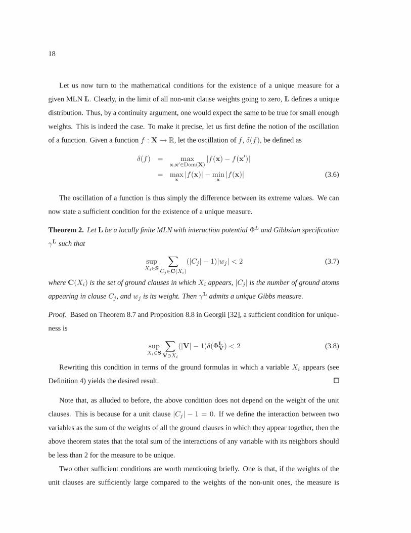
Let us now turn to the mathematical conditions for the existence of a unique measure for a
given MLN L. Clearly, in the limit of all non-unit clause weights going to zero,L defines a unique
distribution. Thus, by a continuity argument, one would expect the same to be true for small enough
weights. This is indeed the case. To make it precise, let us first define the notion of the oscillation
of a function. Given a functionf : X→ R, let the oscillation off , δ(f), be defined as
δ(f) = maxx,x′∈Dom(X)
|f(x)− f(x′)|
= maxx|f(x)| −min
x|f(x)| (3.6)
The oscillation of a function is thus simply the difference between its extreme values. We can
now state a sufficient condition for the existence of a uniquemeasure.
Theorem 2. LetL be a locally finite MLN with interaction potentialΦL and Gibbsian specification
γL such that
supXi∈S
∑
Cj∈C(Xi)
(|Cj | − 1)|wj | < 2 (3.7)
whereC(Xi) is the set of ground clauses in whichXi appears,|Cj | is the number of ground atoms
appearing in clauseCj, andwj is its weight. ThenγL admits a unique Gibbs measure.
Proof. Based on Theorem 8.7 and Proposition 8.8 in Georgii [32], a sufficient condition for unique-
ness is
supXi∈S
∑
V∋Xi
(|V| − 1)δ(ΦL
V) < 2 (3.8)
Rewriting this condition in terms of the ground formulas in which a variableXi appears (see
Definition 4) yields the desired result.
Note that, as alluded to before, the above condition does notdepend on the weight of the unit
clauses. This is because for a unit clause|Cj | − 1 = 0. If we define the interaction between two
variables as the sum of the weights of all the ground clauses in which they appear together, then the
above theorem states that the total sum of the interactions of any variable with its neighbors should
be less than 2 for the measure to be unique.
Two other sufficient conditions are worth mentioning briefly. One is that, if the weights of the
unit clauses are sufficiently large compared to the weights of the non-unit ones, the measure is

19
unique. Intuitively, the unit terms “drown out” the interactions, rendering the variables approxi-
mately independent. The other condition is that, if the MLN is a one-dimensional lattice, it suffices
that the total interaction between the variables to the leftand right of any arc be finite. This corre-
sponds to the ergodicity condition for a Markov chain.
3.3.4 Non-unique MLNs
At first sight, it might appear that non-uniqueness is an undesirable property, and non-unique MLNs
are not an interesting object of study. However, the non-unique case is in fact quite important,
because many phenomena of interest are represented by MLNs with non-unique measures (for ex-
ample, very large social networks with strong word-of-mouth effects). The question of what these
measures represent, and how they relate to each other, then becomes important. This is the subject
of this section.
The first observation is that the set of all Gibbs measuresG(γL) is convex. That is, ifµ, µ′ ∈
G(γL) thenν ∈ G(γL), whereν = sµ + (1− s)µ′, s ∈ (0, 1). This is easily verified by substituting
ν in Equation 3.4. Hence, the non-uniqueness of a Gibbs measure implies the existence of infinitely
many consistent Gibbs measures. Further, many properties of the setG(γL) depend on the set of
extreme Gibbs measuresex G(γL), whereµ ∈ ex G(γL) if µ ∈ G(γL) cannot be written as a linear
combination of two distinct measures inG(γL).
An important notion to understand the properties of extremeGibbs measures is the notion of a
tail event. Consider a subsetS′ of S. Let σ(S′) denote theσ-algebra generated by the set of basic
events involving only variables inS′. Then we define the tailσ-algebraT as
T =⋂
X∈X
σ(SX) (3.9)
Any event belonging toT is called a tail event.T is precisely the set of events which do not
depend on the value of any finite set of variables, but rather only on the behavior at infinity. For
example, in the infinite tosses of a coin, the event that ten consecutive heads come out infinitely
many times is a tail event. Similarly, in the lattice examplein the previous section, the event that
a finite number of variables have the value 1 is a tail event. Events inT can be thought of as
representing macroscopic properties of the system being modeled.

20
Definition 9. A measureµ is trivial on aσ-algebraE if µ(E) = 0 or 1 for all E ∈ E .
The following theorem (adapted from Theorem 7.8 in Georgii [32]) describes the relationship
between the extreme Gibbs measures and the tailσ-algebra.
Theorem 3. LetL be a locally finite MLN, andγL denote the corresponding Gibbsian specification.
Then the following results hold:
1. A measureµ ∈ ex G(γL)) iff it is trivial on the tail σ-algebraT .
2. Each measureµ is uniquely determined by its behavior on the tailσ-algebra, i.e., ifµ1 = µ2
onT thenµ1 = µ2.
It is easy to see that each extreme measure corresponds to some particular value for all the macro-
scopic properties of the network. In physical systems, extreme measures correspond to phases of
the system (e.g., liquid vs. gas, or different directions ofmagnetization), and non-extreme mea-
sures correspond to probability distributions over phases. Uncertainty over phases arises when our
knowledge of a system is not sufficient to determine its macroscopic state. Clearly, the study of
non-unique MLNs beyond the highly regular ones statisticalphysicists have focused on promises to
be quite interesting. In the next section we take a step in this direction by considering the problem
of satisfiability in the context of MLN measures.
3.4 Satisfiability and Entailment
Richardson and Domingos [86] showed that, in finite domains,first-order logic can be viewed as
the limiting case of Markov logic when all weights tend to infinity, in the following sense. If we
convert a satisfiable knowledge baseK into an MLNLK by assigning the same weightw →∞ to
all clauses, thenLK defines a uniform distribution over the worlds satisfyingK. Further,K entails
a formulaα iff LK assigns probability 1 to the set of worlds satisfyingα (Proposition 4.3). In this
section we extend this result to infinite domains.
Consider an MLNL such that each clause in its CNF form has the same weightw. In the
limit w → ∞, L does not correspond to a valid Gibbsian specification, sincethe Hamiltonians
defined in Equation 3.2 are no longer finite. Revisiting Equation 3.5 in the limit of all equal infinite
clause weights, the limiting conditional distribution is equi-distribution over those configurationsX

21
which satisfy the maximum number of clauses givenSX = y. It turns out we can still talk about
the existence of a measure consistent with these conditional distributions, because they constitute
a valid specification (though not Gibbsian) under the same conditions as in the finite weight case.
We omit the details and proofs for lack of space; they can be found in Singla and Domingos [97].
Existence of a measure follows as in the case of finite weightsbecause of the locality of conditional
distributions. We now define the notion of asatisfying measure, which is central to the results
presented in this section.
Definition 10. Let L be a locally finite MLN. Given a clauseCi ∈ B(L), let Vi denote the set
of Boolean variables appearing inCi. A measureµ ∈ G(γL) is said to be asatisfying measure
for L if, for every ground clauseCi ∈ B(L), µ assigns non-zero probability only to the satisfying
assignments of the variables inCi, i.e., µ(Vi = vi) > 0 implies thatVi = vi is a satisfying
assignment forCi. S(γL) denotes the set of all satisfying measures forL.
Informally, a satisfying measure assigns non-zero probability only to those worlds which are
consistent with all the formulas inL. Intuitively, existence of a satisfying measure forL should be
in some way related to the existence of a satisfying assignment for the corresponding knowledge
base. Our next theorem formalizes this intuition.
Theorem 4. LetK be a locally finite knowledge base, and letL∞ be the MLN obtained by assigning
weightw → ∞ to all the clauses inK. Then there exists a satisfying measure forL∞ iff K is
satisfiable. Mathematically,
|S(γL∞)| > 0 ⇔ Satisfiable(K) (3.10)
Proof. Let us first prove that existence of a satisfying measure implies satisfiability ofK. This is
equivalent to proving that unsatisfiability ofK implies non-existence of a satisfying measure. Let
K be unsatisfiable. Equivalently,B(K), the Herbrand base ofK, is unsatisfiable. By Herbrand’s
theorem, there exists a finite set of ground clausesC ⊆ B(K) that is unsatisfiable. LetV denote the
set of variables appearing inC. Then every assignmentv to the variables inV violates some clause
in C. Letµ denote a measure forL∞. Sinceµ is a probability measure,∑
v∈Dom(V) µ(V = v) = 1.
Further, sinceV is finite, there exists somev ∈ Dom(V) such thatµ(V = v) > 0. Let Ci ∈ C be
some clause violated by the assignmentv (every assignment violates some clause). LetVi denote

22
the set of variables inCi andvi be the restriction of assignmentv to the variables inVi. Thenvi
is an unsatisfying assignment forCi. Further,µ(Vi = vi) ≥ µ(V = v) > 0. Henceµ cannot be
a satisfying measure forL∞. Since the above argument holds for anyµ ∈ G(γL∞), there does not
exist a satisfying measure forL∞ whenK is unsatisfiable.
Next, we need to prove that satisfiability ofK implies existence of a satisfying measure. We
will only give a proof sketch here; the full proof can be foundin Singla and Domingos [97]. LetK
be satisfiable. Now, consider a finite subsetX of the variables defined byL∞. GivenX, let ∆X
denote the set of those probability distributions overX which assign non-zero probability only to the
configurations which are partial satisfying assignments ofK. We will call ∆X the set of satisfying
distributions overX. ∆X is a compact set. LetY denote the set of neighbors of the variables in
X. We defineFX : ∆Y → ∆X to be the function which maps a satisfying distribution overY to a
satisfying distribution overX given the conditional distributionγL∞
X(X|SX). The mapping results
in a satisfying distribution overX because, in the limit of all equal infinite weights, the conditional
distribution overX is non-zero only for the satisfying assignments ofX. Since∆Y is compact, its
image under the continuous functionFX is also compact.
Given Xi ⊂ Xj and their neighbors,Yi andYj respectively, we show that ifπXj∈ ∆Xj
is in the image of∆YjunderFXj
, thenπXi=∑
Xj−XiπXj
is in the image of∆XiunderFXi
.
This process can then be repeated for ever-increasing setsXk ⊃ Xi. This defines a sequence
(Tji )
j=∞j=i of non-empty subsets of satisfying distributions overXi. Further, it is easy to show that
∀k Tk+1i ⊆ Tk
i . Since eachTki is compact and non-empty, from the theory of compact sets we
obtain that the countably infinite intersectionTi =⋂j=∞
j=i Tji is also non-empty.
Let (X1,X2, . . . ,Xk, . . .) be some ordering of the variables defined byL∞, and letXk =
X1,X2, . . . Xk. We now define a satisfying measureµ as follows. We defineµ(X1) to be some
element ofT1. Givenµ(Xk), we defineµ(Xk+1) to be that element ofTk+1 whose marginal is
µ(Xk) (such an element always exists, by construction). For an arbitrary set of variablesX, let k
be the smallest index such thatX ⊆ Xk, and defineµ(X) =∑
Xk\Xµ(Xk). We show thatµ
defined in such a way satisfies the properties of a probabilitymeasure (see Section 3.2). Finally,µ
is a satisfying measure because∀k µ(Xk) ∈ Tk and eachTk is a set of satisfying distributions over
Xk.

23
Corollary 11. LetK be a locally finite knowledge base. Letα be a first-order formula, andLα∞ be
the MLN obtained by assigning weightw → ∞ to all clauses inK ∪ ¬α. ThenK entailsα iff
Lα∞ has no satisfying measure. Mathematically,
K |= α ⇔ |S(γLα∞)| = 0 (3.11)
Thus, for locally finite knowledge bases with Herbrand interpretations, first-order logic can
be viewed as the limiting case of Markov logic when all weights tend to infinity. Whether these
conditions can be relaxed is a question for future work.
3.5 Relation to Other Approaches
A number of relational representations capable of handlinginfinite domains have been proposed in
recent years. Generally, they rely on strong restrictions to make this possible. To our knowledge,
Markov logic is the most flexible language for modeling infinite relational domains to date. In this
section we briefly review the main approaches.
Stochastic logic programs [69] are generalizations of probabilistic context-free grammars. PCFGs
allow for infinite derivations but as a result do not always represent valid distributions [8]. In SLPs
these issues are avoided by explicitly assigning zero probability to infinite derivations. Similar re-
marks apply to related languages like independent choice logic [80] and PRISM [90].
Many approaches combine logic programming and Bayesian networks. The most advanced one
is arguably Bayesian logic programs [46]. Kersting and De Raedt show that, if all nodes have a finite
number of ancestors, a BLP represents a unique distribution. This is a stronger restriction than finite
neighborhoods. Richardson and Domingos [86] showed how BLPs can be converted into Markov
logic without loss of representational efficiency.
Jaeger [41] shows that probabilistic queries are decidablefor a very restricted language where
a ground atom cannot depend on other groundings of the same predicate. Jaeger shows that if this
restriction is removed queries become undecidable.
Recursive probability models are a combination of Bayesiannetworks and description logics
[78]. Like Markov logic, RPMs require finite neighborhoods,and in fact existence for RPMs can
be proved succinctly by converting them to Markov logic and applying Theorem 1. Pfeffer and
Koller show that RPMs do not always represent unique distributions, but do not study conditions

24
for uniqueness. Description logics are a restricted subsetof first-order logic, and thus MLNs are
considerably more flexible than RPMs.
Contingent Bayesian networks [65] allow infinite ancestors, but require that, for each variable
with infinite ancestors, there exist a set of mutually exclusive and exhaustive contexts (assignments
to finite sets of variables) such that in every context only a finite number of ancestors affect the
probability of the variable. This is a strong restriction, excluding even simple infinite models like
backward Markov chains [78].
Multi-entity Bayesian networks are another relational extension of Bayesian networks [52].
Laskey and Costa claim that MEBNs allow infinite parents and arbitrary first-order formulas, but the
definition of MEBN explicitly requires that, for each atomX and increasing sequence of substates
S1 ⊂ S2 ⊂ . . ., there exist a finiteN such thatP (X|Sk) = P (X|SN ) for k > N . This assumption
necessarily excludes many dependencies expressible in first-order logic (e.g.,∀x ∃!y Loves(y, x)).
Further, unlike in Markov logic, first-order formulas in MEBNs must be hard (and consistent).
Laskey and Costa do not specify a language for specifying conditional distributions; they simply
assume that a terminating algorithm for computing them exists. Thus the question of what infinite
distributions can be specified by MEBNs remains open.
3.6 Conclusion
In this chapter, we extended the semantics of Markov logic toinfinite domains using the theory
of Gibbs measures. We gave sufficient conditions for the existence and uniqueness of a measure
consistent with the local potentials defined by an MLN. We also described the structure of the set of
consistent measures when it is not a singleton, and showed how the problem of satisfiability can be
cast in terms of MLN measures.

25
Chapter 4
LAZY INFERENCE
4.1 Introduction
Statistical relational models are defined over objects and relations in the domain of interest, and
hence have to support inference over them. We will refer to such domains as relational domains.
A straightforward approach to inference in relational domains is to first propositionalize the theory,
followed by satisfiability testing. As we will show, MAP/MPEinference in these domains can
be reduced to the problem of weighted satisfiability testing. The theory is first propositionalized
(e.g., the ground Markov network is created, in the case of Markov logic) and then standard SAT
solvers are used over the propositionalized theory. This approach has been given impetus by the
development of very fast solvers like WalkSAT [91] and zChaff [68]. Despite its successes, the
applicability of this approach to complex relational problems is still severely limited by at least one
key factor: the exponential memory cost of propositionalization. To apply a satisfiability solver, we
need to create a Boolean variable for every possible grounding of every predicate in the domain,
and a propositional clause for every grounding of every first-order clause. Ifn is the number of
objects in the domain andr is the highest clause arity, this requires memory on the order of nr.
Clearly, even domains of moderate size are potentially problematic, and large ones are completely
infeasible. This becomes an even bigger problem in the context of learning, where inference has to
be performed over and over again. We will revisit this issue in Chapter 6.
In this dissertation, we propose two ways to overcome the problem described above. The first
one, described in this chapter, can be characterized as lazyinference. The basic idea in lazy infer-
ence is to ground out the theory lazily, creating only those clauses and atoms which are actually
considered at the time of the inference. The next chapter will present another technique called lifted
inference, which is conceptually similar to the idea of resolution in first-order logic. The key idea
in lifted inference is to perform inference together for a set (cluster) of nodes about which we have
the same information.
26
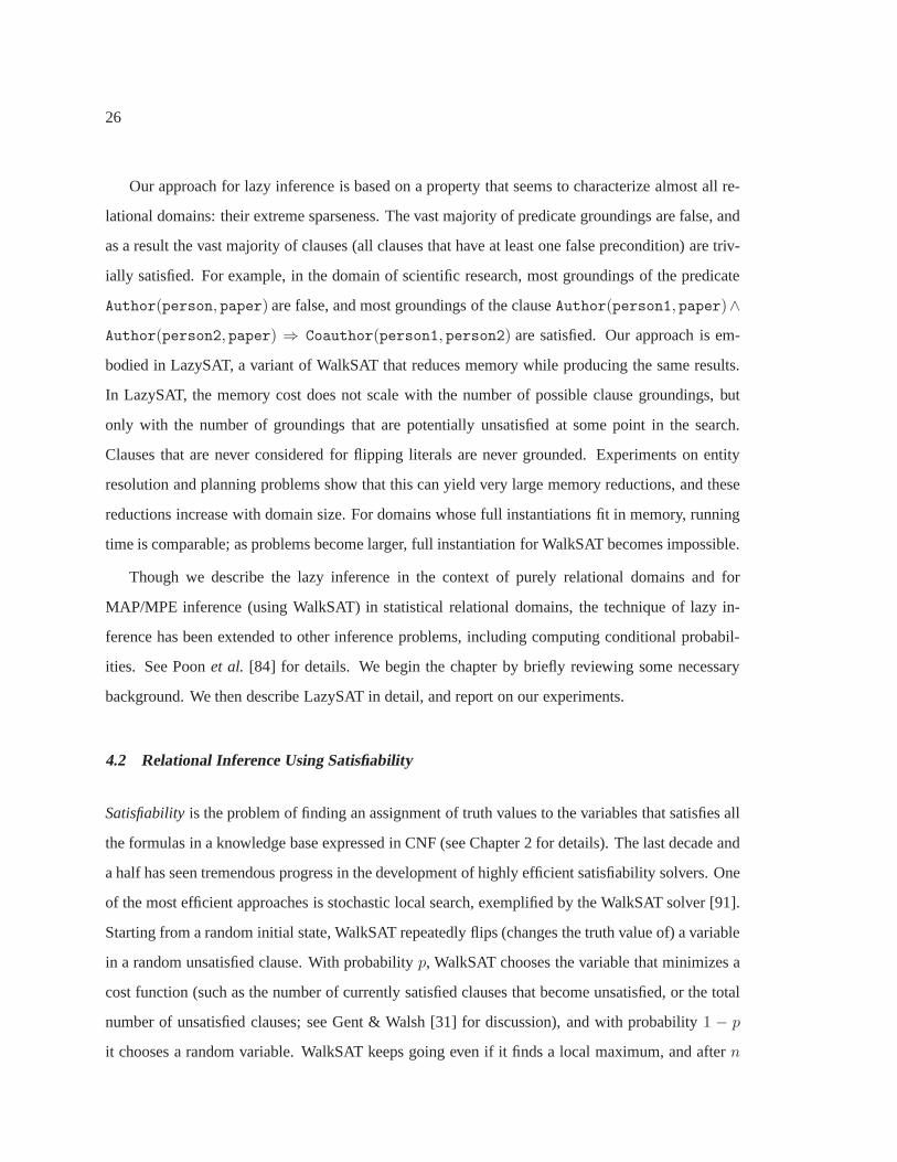
Our approach for lazy inference is based on a property that seems to characterize almost all re-
lational domains: their extreme sparseness. The vast majority of predicate groundings are false, and
as a result the vast majority of clauses (all clauses that have at least one false precondition) are triv-
ially satisfied. For example, in the domain of scientific research, most groundings of the predicate
Author(person, paper) are false, and most groundings of the clauseAuthor(person1, paper)∧
Author(person2, paper) ⇒ Coauthor(person1, person2) are satisfied. Our approach is em-
bodied in LazySAT, a variant of WalkSAT that reduces memory while producing the same results.
In LazySAT, the memory cost does not scale with the number of possible clause groundings, but
only with the number of groundings that are potentially unsatisfied at some point in the search.
Clauses that are never considered for flipping literals are never grounded. Experiments on entity
resolution and planning problems show that this can yield very large memory reductions, and these
reductions increase with domain size. For domains whose full instantiations fit in memory, running
time is comparable; as problems become larger, full instantiation for WalkSAT becomes impossible.
Though we describe the lazy inference in the context of purely relational domains and for
MAP/MPE inference (using WalkSAT) in statistical relational domains, the technique of lazy in-
ference has been extended to other inference problems, including computing conditional probabil-
ities. See Poonet al. [84] for details. We begin the chapter by briefly reviewing some necessary
background. We then describe LazySAT in detail, and report on our experiments.
4.2 Relational Inference Using Satisfiability
Satisfiabilityis the problem of finding an assignment of truth values to the variables that satisfies all
the formulas in a knowledge base expressed in CNF (see Chapter 2 for details). The last decade and
a half has seen tremendous progress in the development of highly efficient satisfiability solvers. One
of the most efficient approaches is stochastic local search,exemplified by the WalkSAT solver [91].
Starting from a random initial state, WalkSAT repeatedly flips (changes the truth value of) a variable
in a random unsatisfied clause. With probabilityp, WalkSAT chooses the variable that minimizes a
cost function (such as the number of currently satisfied clauses that become unsatisfied, or the total
number of unsatisfied clauses; see Gent & Walsh [31] for discussion), and with probability1 − p
it chooses a random variable. WalkSAT keeps going even if it finds a local maximum, and aftern

27
flips restarts from a new random state. The whole procedure isrepeatedm times. WalkSAT can
solve random problems with hundreds of thousands of variables in a fraction of a second, and hard
ones in minutes. However, it cannot distinguish between an unsatisfiable CNF and one that takes
too long to solve.
The MaxWalkSAT [44] algorithm extends WalkSAT to the weighted satisfiability problem,
where each clause has a weight and the goal is to maximize the sum of the weights of satisfied
clauses. (Systematic solvers have also been extended to weighted satisfiability, but tend to work less
well.) Park [75] showed how the problem of finding the most likely state of a Bayesian network
given some evidence can be efficiently solved by reduction toweighted satisfiability. WalkSAT is
essentially the special case of MaxWalkSAT obtained by giving all clauses the same weight. For
simplicity, in this dissertation we will just treat them as one algorithm, called WalkSAT, with the
sum of the weights ofunsatisfiedclauses as the cost function that we seek to minimize. Algorithm 1
gives pseudo-code for WalkSAT. DeltaCost(v) computes the change in the sum of weights of un-
satisfied clauses that results from flipping variablev in the current solution. Uniform(0,1) returns a
uniform deviate from the interval[0, 1].
First-order logic (FOL) allows us to explicitly represent adomain’s relational structure (see
Chapter 2). Objects are represented by constants, and the relations among them by predicates. As
mentioned earlier, we make the assumptions of unique names,domain closure and known functions.
A predicate or formula isgroundedby replacing all its variables by constants.Propositionalization
is the process of replacing a first-order KB by an equivalent propositional one. In finite domains,
this can be done by replacing each universally (existentially) quantified formula with a conjunction
(disjunction) of all its groundings. A first-order KB is satisfiable iff the equivalent propositional
KB is satisfiable. Hence, inference over a first-order KB can be performed by propositionalization
followed by satisfiability testing.
Turning now to the problem of inference in statistical relational domains, let us revisit Equa-
tion 2.3, which gives the distribution defined by a Markov logic network. The probability of a state
x in a ground Markov network can be written asP (x) = (1/Z) exp (∑
i wifi(x)), whereZ is the
normalization constant,wi is the weight of theith clause,fi = 1 if the ith clause is true, andfi = 0
otherwise. Finding the most probable state of a grounded MLNgiven some evidence is thus an
instance of weighted satisfiability.

28
Algorithm 1 WalkSAT (weightedclauses, max flips, max tries, target, p)vars← variables inweightedclauses
for i ← 1 tomax tries do
soln← a random truth assignment tovars
cost← sum of weights of unsatisfied clauses insoln
for i ← 1 tomax flips do
if cost≤ target then
return “Success, solution is”,soln
end if
c← a randomly chosen unsatisfied clause
if Uniform(0,1)< p then
vf ← a randomly chosen variable fromc
else
for each variablev in c do
compute DeltaCost(v)
end for
vf ← v with lowest DeltaCost(v)
end if
soln← solnwith vf flipped
cost← cost+ DeltaCost(vf )
end for
end for
return “Failure, best assignment is”, bestsoln found

29
The LazySAT algorithm we develop in this dissertation can beused to scale relational inference
to much larger domains than standard WalkSAT. As mentioned earlier, the ideas in LazySAT are
also directly applicable to scaling up the computation of marginal and conditional probabilities in
statistical relational domains, using Markov chain Monte Carlo algorithms [84].
4.3 Memory-Efficient Inference
The LazySAT algorithm reduces the memory required by satisfiability testing in relational domains
by taking advantage of their sparseness. Because the great majority of ground atoms are false, most
clauses are satisfied throughout the search, and never need to be considered. LazySAT grounds
clauses lazily, at each step in the search adding only the clauses that could become unsatisfied. In
contrast, WalkSAT grounds all possible clauses at the outset, consuming time and memory expo-
nential in their arity.
Algorithm 2 gives pseudo-code for LazySAT, highlighting the places where it differs from Walk-
SAT. LazySAT inputs an MLN (or a pure first-order KB, in which case all clauses are assigned
weight 1) and a database (DB). A database is a set of ground atoms. (For example, in planning
problems the database is the set of ground atoms describing the initial and goal states. In prob-
abilistic inference, the database is the evidence we condition on.) An evidence atomis either a
ground atom in the database, or a ground atom that is false by the closed world assumption (i.e., it
is a grounding of an evidence predicate, and does not appear in the database). The truth values of
evidence atoms are fixed throughout the search, and ground clauses are simplified by removing the
evidence atoms. LazySAT maintains a set ofactive atomsand a set ofactive clauses. A clause is
active if it can be made unsatisfied by flipping zero or more of its active atoms. (Thus, by definition,
an unsatisfied clause is always active.) An atom is active if it is in the initial set of active atoms,
or if it was flipped at some point in the search. The initial active atoms are all those appearing in
clauses that are unsatisfied if only the atoms in the databaseare true, and all others are false. We
use dynamic arrays to store the active clauses and the atoms in them. The unsatisfied clauses are
obtained by simply going through each possible grounding ofall the first-order clauses and ma-
terializing the groundings that are unsatisfied; search is pruned as soon the partial grounding of a
clause is satisfied. Given the initial active atoms, the definition of active clause requires that some

30
clauses become active, and these are found using a similar process (with the difference that, instead
of checking whether a ground clause is unsatisfied, we check whether it should be active).1 Each
run of LazySAT is initialized by assigning random truth values to the active atoms. This differs from
WalkSAT, which assigns random values to all atoms. However,the LazySAT initialization is a valid
WalkSAT initialization, and we have verified experimentally that the two give very similar results.
Given the same initialization, the two algorithms will produce exactly the same results.
At each step in the search, the variable that is flipped is activated, as are any clauses that by
definition should become active as a result. When evaluatingthe effect on cost of flipping a variable
v, if v is active then all of the relevant clauses are already active, and DeltaCost(v) can be computed
as in WalkSAT. Ifv is inactive, DeltaCost(v) needs to be computed using the knowledge base. (In
principle, repeated calculation of this kind can be avoidedby activating a variable (and its clauses)
when it is first encountered, but we found the time savings from this to be outweighed by the added
memory cost.) This is done by retrieving from the KB all first-order clauses containing the predicate
that v is a grounding of, and grounding each such clause with the constants inv and all possible
groundings of the remaining variables. As before, we prune search as soon as a partial grounding is
satisfied, and add the appropriate multiple of the clause weight to DeltaCost(v). (A similar process
is used to activate clauses.) While this process is costlierthan using pre-grounded clauses, it is
amortized over many tests of active variables. In typical satisfiability problems, a small core of
“problem” clauses is repeatedly tested, and when this is thecase LazySAT will be quite efficient.
At each step, LazySAT flips the same variable that WalkSAT would, and hence the result of the
search is the same. The memory cost of LazySAT is on the order of the maximum number of clauses
active at the end of a run of flips. (The memory required to store the active atoms is dominated by
the memory required to store the active clauses, since each active atom appears in at least one active
clause.) In the current version of LazySAT, clauses and atoms are never deactivated, but this could
easily be changed to save memory without affecting the output by periodically reinitializing the
active sets (using the current truth values of all non-evidence atoms, instead of all false). In our
experiments this was not necessary, but it could be quite useful in very long searches.
1Although for simplicity the pseudo-code does not show this,the initial set of active clauses and active atoms can besaved and reused for each restart, saving time.

31
4.4 Experiments
We performed experiments on two entity resolution domains and a planning domain to compare
the memory usage and running time of LazySAT and WalkSAT. We implemented LazySAT as an
extension of the Alchemy system [48], and used Kautzet al.’s (1997) implementation of MaxWalk-
SAT, included in Alchemy. When propositionalizing a problem for WalkSAT, we did not ground
clauses that are always true given the evidence, and this saved a significant amount of memory.
Since the two algorithms can be guaranteed to produce the same results by using the same random
initialization for both, we do not report solution quality.In all the experiments we ran WalkSAT
and LazySAT for a million flips, with no restarts. The experiments were run on a cluster of nodes,
each node having 3.46 GB of RAM and two processors running at 3GHz. All results reported are
averages over five random problem instances.
4.4.1 Entity Resolution
In many domains, the entities of interest are not uniquely identified, and we need to determine
which observations correspond to the same entity. For example, when merging databases we need
to determine which records are duplicates. This problem is of crucial importance to many large
scientific projects, businesses, and government agencies,and has received increasing attention in
the AI community in recent years. We will talk about this problem in detail in Chapter 7. We
used two publicly available citation databases in our experiments: McCallum’s Cora database as
segmented by Bilenko and Mooney [4]. This dataset contains 1295 citations and is extracted from
the original Cora database of over 50,000 citations. We further cleaned this dataset to fill in some
missing values and correct some labels. The cleaned versioncontained references to 132 distinct
research papers and is publicly available on the Alchemy [48] website. Bibserv dataset is available
from BibServ.org, which combines CiteSeer, DBLP, and user-donated databases. BibServ contains
approximately half a million citations. We used the user-donated subset of BibServ, with 21,805
citations. The inference task was to de-duplicate citations, authors and venues (i.e., to determine
which pairs of citations refer to the same underlying paper,and similarly for author fields and venue
fields). We used the Markov logic network constructed by Singla and Domingos [93], ignoring
clauses with negative weight. Clauses weights were learnt on the Cora dataset using their algorithm

32
and used on both Cora and Bibserv. (We could not learn weightson BibServ because the data is not
labeled.)
This contains 33 first-order clauses stating regularities such as: if two fields have high TF-IDF
similarity, they are (probably) the same; if two records arethe same, their fields are the same,
and vice-versa; etc. Crucially, we added the transitivity rule with a very high weight:∀x, y, z
x = y ∧ y = z ⇒ x = z. This rule is used in anad hocway in most entity resolution systems, and
greatly complicates inference. The highest clause arity, after conditioning on evidence, was three.
We varied the number of records from 50 to 500 in intervals of 50, generating five random sub-
sets of the data for each number of records. We ensured that each real cluster in the data was either
completely included in a subset or completely excluded, with the exception of the last one to be
added, which had to be truncated to ensure the required number of records. Figure 4.1 shows how
the total number of clauses grounded by LazySAT and WalkSAT varies with the number of records.
The RAM usage in bytes correlates closely with the number of groundings (e.g., for 250 records
WalkSAT uses 2.1 GB, and LazySAT 288 MB). The memory reduction obtained by LazySAT in-
creases rapidly with the number of records. At 250 records, it is about an order of magnitude.
Beyond this point, WalkSAT runs out of memory. To extrapolate beyond it, we fitted the function
f(x) = axb to both curves, obtaininga = 1.19, b = 2.97 (with R2 = 0.99) for WalkSAT and
a = 6.02, b = 2.34 (with R2 = 0.98) for LazySAT. Using these, on the full Cora database LazySAT
would reduce memory usage by a factor of over 300.
Figure 4.2 compares the speed of the two algorithms in average flips per second (i.e., total num-
ber of flips over total running time). LazySAT is somewhat faster than WalkSAT for low numbers of
records, but by 250 records this advantage has disappeared.Recall that total running time has two
main components: initialization, where LazySAT has the advantage, and variable flipping, where
WalkSAT does. The relative contribution of the two depends on the problem size and total number
of flips. WalkSAT flips variables at a constant rate throughout the search. LazySAT initially flips
them slower, on average, but as more clauses become active its flipping rate increases and converges
to WalkSAT’s.
On BibServ, we formed random subsets of size 50 to 500 recordsusing the same approach as in
Cora, except that instead of using the (unknown) real clusters we formed clusters using the canopy
approach of McCallumet al. [61]. Figure 4.3 shows the number of clause groundings as a function

33
1.6*107
1.2*107
8.0*106
4.0*106
0 0 100 200 300 400 500
No.
Cla
uses
No. Records
LazySATWalkSAT
Figure 4.1: Experimental results on Cora: memory as a function of the number of records
of the number of records. RAM usage behaved similarly, being1.9 GB for WalkSAT and 78 MB
for LazySAT at 250 records. As before, WalkSAT runs out of memory at 250 records. LazySAT’s
memory requirements increase at a much lower rate on this database, giving it a very large advantage
over WalkSAT. Fitting the functionf(x) = axb to the two curves, we obtaineda = 1.02, b =
2.98 (with R2 = 0.99) for WalkSAT anda = 28.15, b = 1.75 (with R2 = 0.98) for LazySAT.
Extrapolating these, on the full BibServ database LazySAT would reduce memory compared to
WalkSAT by a factor of over 400,000. The greater advantage ofLazySAT on BibServ is directly
attributable to its larger size and consequent greater sparseness, and we expect the advantage to be
even greater for larger databases. (To see why larger size leads to greater sparseness, consider for
example the predicateAuthor(person, paper). When the number of papers and authors increases,
its number of true groundings increases only approximatelyproportionally to the number of papers,
while the number of possible groundings increases proportionally to its product by the number of
authors. On a database with thousands of authors, the resulting difference can be quite large.)
Figure 4.4 compares the speeds of the two algorithms. They are similar, with LazySAT being
slightly faster below 100 objects and WalkSAT slightly faster above.

34
1.0*106
1.0*104
1.0*102
1.0 0 100 200 300 400 500
Flip
s/S
ec
No. Records
LazySATWalkSAT
Figure 4.2: Experimental results on Cora: speed as a function of the number of records
1.6*107
1.2*107
8.0*106
4.0*106
0 0 100 200 300 400 500
No.
Cla
uses
No. Records
LazySATWalkSAT
Figure 4.3: Experimental results on Bibserv: memory as a function of the number of records

35
1.0*106
1.0*104
1.0*102
1.0 0 100 200 300 400 500
Flip
s/S
ec
No. Records
LazySATWalkSAT
Figure 4.4: Experimental results on Bibserv: speed as a function of the number of records
1.6*107
1.2*107
8.0*106
4.0*106
0 0 20 40 60 80 100
No.
Cla
uses
No. Blocks
LazySATWalkSAT
Figure 4.5: Experimental results on blocks world: memory asa function of the number of records

36
1.0*106
1.0*104
1.0*102
1.0 0 20 40 60 80 100
Flip
s/S
ec
No. Blocks
LazySATWalkSAT
Figure 4.6: Experimental results on blocks world: speed as afunction of the number of records
4.4.2 Planning
To compare LazySAT and WalkSAT on a pure (unweighted) satisfiability problem, we experimented
on the classical blocks world planning domain, where the goal is to find a sequence of block moves
that transforms the initial stacking of blocks into the goalstacking. Kautz & Selman [43] showed
how to encode planning problems as instances of satisfiability, by writing formulas that specify ac-
tion definitions, frame axioms, etc., and using a database ofground atoms to specify the initial state
and goal state. We used the formulas they wrote for the blocksworld domain (publicly available
at http://www.cs.washington.edu/homes/kautz/satplan/blackbox/satplandist 2001.tar.Z). The max-
imum clause arity was four. All the clauses were assigned unit weight. Given a number of blocks,
we generated random problem instances as follows. We set thenumber of stacks in both the initial
and goal state to the square root of the number of blocks (truncated to the nearest integer). The stacks
were then populated by randomly assigning blocks to them. The number of allowed moves was lib-
erally set to the length of the trivial solution (unstackingand restacking all the blocks). We added
rules to allow null moves, making it possible for the algorithms to find shorter plans. We varied the
number of blocks from 10 to 100 in increments of 10, and generated five random instances for each.

37
Figure 4.5 shows how the number of clauses grounded by the twoalgorithms varies with the number
of blocks. LazySAT once again obtains very large reductions. RAM usage closely paralleled the
number of clauses, being 1.6 GB for WalkSAT and 203 MB for LazySAT at 50 blocks. WalkSAT is
only able to go up 50 blocks, and LazySAT’s gain at this size isabout an order of magnitude. Fitting
the functionf(x) = axb to the two curves, we obtaineda = 2.79, b = 3.90 (with R2 = 0.99)
for WalkSAT, anda = 1869.58, b = 1.68 (with R2 = 0.99) for LazySAT. The difference in the
asymptotic behavior is even more prominent here than in the entity resolution domains.
Figure 4.6 compares the speed of the two algorithms. WalkSATis somewhat faster, but the
difference decreases gradually with the number of blocks.
In all domains, LazySAT reduced memory by an order of magnitude or more at the point that
WalkSAT exceeded available RAM. Most importantly, LazySATmakes it feasible to solve much
larger problems than before.
4.5 Conclusion
Satisfiability testing is very effective for inference in relational domains, but is limited by the expo-
nential memory cost of propositionalization. The LazySAT algorithm overcomes this problem by
exploiting the sparseness of relational domains. Experiments on entity resolution and planning prob-
lems show that it greatly reduces memory requirements compared to WalkSAT, without sacrificing
speed or solution quality.
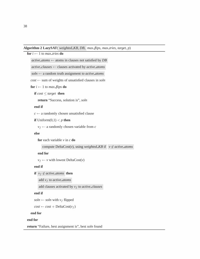
38
Algorithm 2 LazySAT ( weightedKB, DB, maxflips, max tries, target, p)
for i ← 1 tomax tries do
active atoms← atoms in clauses not satisfied byDB
active clauses← clauses activated byactive atoms
soln← a random truth assignment toactive atoms
cost← sum of weights of unsatisfied clauses insoln
for i ← 1 tomax flips do
if cost≤ target then
return “Success, solution is”,soln
end if
c← a randomly chosen unsatisfied clause
if Uniform(0,1)< p then
vf ← a randomly chosen variable fromc
else
for each variablev in c do
compute DeltaCost(v), usingweightedKB if v 6∈ active atoms
end for
vf ← v with lowest DeltaCost(v)
end if
if vf 6∈ active atoms then
addvf to active atoms
add clauses activated byvf to active clauses
end if
soln← solnwith vf flipped
cost← cost+ DeltaCost(vf )
end for
end for
return “Failure, best assignment is”, bestsoln found

39
Chapter 5
LIFTED INFERENCE
5.1 Introduction
In the last chapter, we talked about lazy inference as a way toavoid fully grounding out the network
during inference. But lazy inference still works at the propositional level, in the sense that the
units of operation during inference are ground clauses. In contrast, a key property of first-order
logic is that it allowslifted inference, where queries are answered without materializing all the
objects in the domain (e.g., resolution [87]). Lifted inference is potentially much more efficient than
propositionalized inference (or for that matter even lazy inference), and extending it to probabilistic
logical languages is a desirable goal.
The only approach to lifted probabilistic inference to datewas developed by Poole [81] and
extended by de S. Brazet al. ([20], [21]). (Limited lifted aspects are present in some earlier systems,
like Pfeffer et al.’s [79] SPOOK.) Poole and Brazet al. introduced a lifted version of variable
elimination, the simplest algorithm for inference in probabilistic graphical models. Unfortunately,
variable elimination has exponential cost in the treewidthof the graph, making it infeasible for
most real-world applications. Scalable approximate algorithms for probabilistic inference fall into
three main classes: loopy belief propagation (BP), Monte Carlo methods, and variational methods.
Jaimovichet al. [42] pointed out that, if there is no evidence, BP in probabilistic logical models
can be trivially lifted, because all groundings of the same first-order predicates and features become
indistinguishable.
In this chapter we develop a general framework for lifting a number of probabilistic inference
algorithms including variable elimination and belief propagation. Our approach proceeds by iden-
tifying the subsets of nodes and features (groundings of thefirst-order predicates and features, re-
spectively) that remain indistinguishable even after evidence is taken into account. We call them
themsupernodesandsuperfeatures. The key operations involved in constructing the supernodes
and superfeatures arejoin andproject as defined in the database literature. Supernodes at a given
40
step are joined together to obtain the next round of superfeatures which in turn are projected back to
obtain the new supernodes. The algorithm now operates on these constructs rather than the ground
nodes and features, thereby saving a large number of repeated calculations. Execution of the infer-
ence algorithm may necessitate further splitting of the supernodes and superfeatures, which is done
as the execution proceeds.
We first provide the general framework for lifting and then apply it to specific algorithms: bucket
elimination [22], which generalizes many inference algorithms, including variable elimination and
then to belief propagation and junction tree algorithm. We prove the correctness of our algorithm,
showing that it gives exactly the same results as the ground version. In the case of BP, we show
that there is a unique minimal lifted network (on which lifted BP can be run) for every inference
problem, and that our algorithm returns it. We then extend our algorithm for approximate lifting,
which can provide further gains in time and memory efficiencytrading off some accuracy. The key
idea in approximate lifting is to merge the nodes (features)which are approximately similar to each
other. We formalize this notion approximate similarity anddescribe two ways of constructing the
approximate network.
Our method is applicable to essentially any probabilistic logical language, including approaches
based on Bayesian networks and Markov networks. We will use Markov logic as a concrete example
[86]. Our algorithm is also much simpler than the algorithmsof Poole and Brazet al. We present the
first experimental results for lifted probabilistic inference on a number of real domains. These, and
systematic experiments on synthetic problems, show that lifted probabilistic inference can greatly
outperform the standard propositionalized version.
5.2 Background
As discussed in Chapter 2,Graphical modelscompactly represent the joint distribution of a set of
variablesX = (X1,X2, . . . ,Xn) ∈ X as a product of factors [77]:P (X=x) = 1Z
∏
k gk(xk),
where each factorgk is a non-negative function of a subset of the variablesxk, andZ is a normal-
ization constant. Under appropriate restrictions, the model is aBayesian networkandZ = 1. The
main inference task in graphical models is to compute the conditional probability of some variables
(the query) given the values of some others (the evidence), by summing out the remaining variables.
41
This problem is #P-complete, but becomes tractable if the graph is a tree. A number of inference
algorithms (exact as well as approximate) have been proposed in the literature for carrying out infer-
ence in graphical models. Next, we will present a few of the important inference algorithms which
will become the candidates for our lifting framework in the later part of the chapter.
5.2.1 Bucket Elimination
Bucket elimination [22] is a unifying framework for a variety of inference algorithms. Given a
distribution defined over the set of variablesX using a set of factorsg, the algorithm proceeds by
operating on buckets, where each bucket represents the calculation corresponding to elimination of
a variable in setX. In the beginning, we createn = |V | buckets, one for each variable. Some
orderingb1, b2, . . . , bn of the buckets is chosen. The query variable is placed in the lowest bucket,
i.e.,b1. Given a factorg, it is placed in the bucket with the highest index such that the corresponding
variable appears ing. Bucket elimination now proceeds by eliminating the highest indexed bucket
in turn. All the factors in the bucket being eliminated are multiplied to obtain a single factor. Then
the variable being eliminated is summed out. The resulting factor is placed in the bucket with the
highest index (among the remaining buckets) whose variableappears in the factor. The evidence is
handled slightly differently. In the case of evidence variables, there is no need to multiply and sum
out. The evidence value is substituted into each factor in the bucket, and the factor simplified. The
simplified factor is then placed in the appropriate bucket down the line. The process continues until
only the query bucket remains. At this point, all the factorscan be multiplied together and the bucket
contains the unnormalized probability of the query. The pseudo-code is given in Tables 5.1 and
5.2. Function “AddToBucket” puts the input feature (first argument) into the input bucket (second
argument). Function “ElimNode” performs a pointwise multiplication of the potentials represented
by the input features, sums the input node (variable) out andreturns the resulting feature.
In addition to the problem of estimating probabilities, thebucket elimination framework as de-
scribed above can be used for various other inference tasks such as MPE estimation, MAP estimation
and MEU estimation. This is done by replacing the summation operation in the “ElimNode” func-
tion by a maximization operation (MPE), a combination of summation and maximization (MAP)
or some other such variant (e.g., MEU). A number of algorithms such as directional resolution for
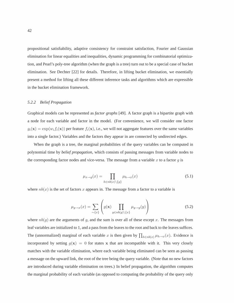
42
propositional satisfiability, adaptive consistency for constraint satisfaction, Fourier and Gaussian
elimination for linear equalities and inequalities, dynamic programming for combinatorial optimiza-
tion, and Pearl’s poly-tree algorithm (when the graph is a tree) turn out to be a special case of bucket
elimination. See Dechter [22] for details. Therefore, in lifting bucket elimination, we essentially
present a method for lifting all these different inference tasks and algorithms which are expressible
in the bucket elimination framework.
5.2.2 Belief Propagation
Graphical models can be represented asfactor graphs[49]. A factor graph is a bipartite graph with
a node for each variable and factor in the model. (For convenience, we will consider one factor
gi(x) = exp(wifi(x)) per featurefi(x), i.e., we will not aggregate features over the same variables
into a single factor.) Variables and the factors they appearin are connected by undirected edges.
When the graph is a tree, the marginal probabilities of the query variables can be computed in
polynomial time bybelief propagation, which consists of passing messages from variable nodes to
the corresponding factor nodes and vice-versa. The messagefrom a variablex to a factorg is
µx→g(x) =∏
h∈nb(x)\g
µh→x(x) (5.1)
wherenb(x) is the set of factorsx appears in. The message from a factor to a variable is
µg→x(x) =∑
∼x
g(x)∏
y∈nb(g)\x
µy→g(y)
(5.2)
wherenb(g) are the arguments ofg, and the sum is over all of these exceptx. The messages from
leaf variables are initialized to 1, and a pass from the leaves to the root and back to the leaves suffices.
The (unnormalized) marginal of each variablex is then given by∏
h∈nb(x) µh→x(x). Evidence is
incorporated by settingg(x) = 0 for statesx that are incompatible with it. This very closely
matches with the variable elimination, where each variablebeing eliminated can be seen as passing
a message on the upward link, the root of the tree being the query variable. (Note that no new factors
are introduced during variable elimination on trees.) In belief propagation, the algorithm computes
the marginal probability of each variable (as opposed to computing the probability of the query only

43
in variable elimination), which is done by sending the messages from the root back to the leaf nodes.
This algorithm can still be applied when the graph has loops,repeating the message-passing until
convergence. Although thisloopybelief propagation has no guarantees of convergence or of giving
the correct result, in practice it often does, and can be muchmore efficient than other methods.
Different schedules may be used for message-passing. Here we assumeflooding, the most widely
used and generally best-performing method, in which messages are passed from each variable to
each corresponding factor and back at each step (after initializing all variable messages to 1).
5.2.3 Junction Tree Algorithm
Belief propagation can also be used for exact inference in arbitrary graphs, by combining nodes
until a tree is obtained. Although this suffers from the samecombinatorial explosion as variable
elimination, it is the basis of the most widely used exact inference algorithm: the junction tree
algorithm. In this algorithm, a tree data structure called the junction tree is first constructed [77].
Each node of the junction tree represents a set of nodes in theoriginal graph. A junction tree is
characterized by the running intersection property i.e. given two nodesv andw in the junction tree,
each node on the unique path betweenv andw contains the intersection of the nodes represented by
v andw. To construct a junction tree, the original graph is first converted into a chordal graph. A
chordal graph is a graph containing no chordless cycles. Thenodes in the junction tree are simply
the maximal cliques in the chordal graph. The construction of the junction tree is analogous to the
variable elimination process. Each variable and all its neighbors form a clique, and each maximal
clique is connected to a parent clique, typically the one with which it shares the largest number
of variables [22]. Each potential is assigned to a node (maximal clique) containing the clique it is
over. Each edge (separator) of the junction tree representsthe intersection of the two clique nodes it
connects. Given a junction tree, the marginals of all the nodes can be now computed using a message
passing scheme analogous to the one described in the previous section. Messages are passed from
a clique to its neighbor by first summing out the variables notin the separator and then multiplying
the new separator marginal into the neighbor’s distribution.

44
5.3 A General Framework for Lifting
We begin with some necessary definitions and theorems. Theseassume the existence of an MLN
M, set of constantsC, and evidence databaseE (set of ground literals). Given an algorithmA for
manipulating the variables, features and probabilities associated with them, we define the following
constructs.
Definition 12. A supernodeis a set of groundings of a predicate that can be treated as indistin-
guishable from each other during the execution of algorithmA, givenM, C andE. We say two
groundingsn1 andn2 are indistinguishable if the calculations involved in processingn1 are iden-
tical to the those involved in processingn2. The supernodes of a predicate form a partition of its
groundings.
A superfeatureis a set of groundings of a clause that all can be treated as indistinguishable from
each other during the execution ofA, givenM, C andE, where indistinguishable groundings are
as defined before. The superfeatures of a clause form a partition of its groundings.
Note that a supernode (superfeature) can be thought of as defining a relation over the domains
of the variables appearing in the corresponding predicate (clause). For simplicity, our definitions
and explanation of the algorithm will assume that each predicate appears at most once in any given
MLN clause. We will then describe how to handle multiple occurrences of a predicate in a clause.
The basis of our lifting framework will be to identify all thenodes which have the same marginal
probability. This brings us to the notion of probability equivalence.
Definition 13. Two ground atoms (nodes) areprobability equivalentif they have the same marginal
probabilities. A supernodeN is said to be probability equivalent if each pair of ground atoms in it
is probability equivalent.
The process of lifting in our framework essentially corresponds to starting with a coarse set of
supernodes and superfeatures, and then iteratively refining them, so as to separate out the nodes
which are not probability equivalent. Lifting allows us to treat all the nodes which can be processed
in a similar manner (at any given step of the algorithm) as a group, thereby reducing (as in some
cases completely eliminating) the amount of redundant calculation. At the end of the lifting process,
we will obtain a set of supernodes which are probability equivalent modulo the inference algorithm,

45
i.e., each ground node in a supernode will have the same probability under the given inference
algorithm. To manipulate the supernodes and superfeaturesas described above, we will need to
define the following basic constructs.
Definition 14. Given a set of supernodesN1,N2, . . . ,Nk respectively belonging to the set of
predicatesP1, P2, . . . , Pk, join(N1,N2, . . . ,Nk) returns a relation defined over the domains
D1,D2, . . . ,Dl, where eachDi represents the domain of a variable in the set of unique variables
appearing in the predicatesP1, P2, . . . , Pk. The relation is obtained by forming a cartesian product
of the relations defined by the supernodesN1,N2, . . . ,Nk, and selecting the tuples in which the
corresponding arguments agree with each other.
Definition 15. Let F be a superfeature andC be the corresponding clause. Given a predicateP
appearing inC, project(F ,P ) returns a relation defined over the domainsD1,D2, . . . ,Dk where
Di’s are the domains of the variables appearing inP . The relation is obtained by restricting the
tuples inF onto the variables inP . Given a ground atomn1 corresponding to predicateP , the
projection countof F onto n1 is defined as the number ofF tuples that results inn1 when the
operation project(F ,P ) is applied.
Next, we will define the notion of a stable configuration amonga set of supernodes and su-
perfeatures, which will be central to our description of thelifting framework. Intuitively, a set of
supernodes and superfeatures are in a stable configuration if (a) the superfeatures can be constructed
by joining the supernodes and (b) each ground predicate in a supernode is involved in the same num-
ber of the same kind of superfeatures. Formalizing this notion, we give the following definition.
Definition 16. Let N be some set of supernodes andF be the set of superfeatures. We say that
N and F are in a stable configurationwith respect to each other if the following conditions are
satisfied.
• Given a superfeatureF ∈ F, F can be obtained by a join of the supernodes in the set
N1, N2, . . . , Nk, where eachNi ∈ N.
• Given any two ground atomsn1, n2 belonging to a supernodeN ∈ N, n1 andn2 have the
same projection counts for every superfeatureF ∈ F.

46
To handle clauses with multiple occurrences of a predicate,when projecting superfeatures onto
supernodes, a separate count is maintained for each occurrence and the counts have to match up for
each occurrence. We are now ready to describe the process of constructing a network of supernodes
and superfeatures which are in a stable configuration. Initially, the groundings of each predicate fall
into three groups: known true, known false and unknown. (Oneor two of these may be empty.)
Each such group constitutes an initial supernode. All groundings of a clause whose atoms have
the same combination of truth values (true, false or unknown) now can be thought of as forming
a superfeature. In turn, all ground atoms that appear in the same number of same kind of super-
features form a supernode. As the effect of the evidence propagates through the network, finer and
finer supernodes and superfeatures are created. Thus, the creation of supernodes and superfeatures
proceeds by alternating between two steps:
1. Form superfeatures by doing joins of the supernodes.
2. Form supernodes by projecting superfeatures down to their predicates, and merging atoms
with the same projection counts.
The first step corresponds to ajoin operation. It takes as input the current set of superfeatures and
supernodes and returns the finer set of superfeatures. Each superfeatureF is split into finer super-
features by doing a join over the current set of supernodes. Figure 5.3 presents the pseudo-code.
The second step corresponds to theprojectoperation. It takes as input the current set superfeatures
and returns the finer set of supernodes. For each predicateP , the finer supernodes are obtained by
projecting every superfeature inF ∈ F ontoP and merging those tuples with have the same counts
from every superfeatureF . Figure 5.4 presents the pseudo-code. Once a stable configuration of
supernodes and superfeatures is reached, we perform one step of the original algorithm, i.e., elimi-
nating a variable (a supernode) in case of variable elimination (VE) or passing a message in the case
of belief propagation (BP). This advances the algorithm by one step, where is performed at the level
of supernodes/superfeatures, thereby saving a large number of repeated calculations. This step in
some cases may result in creation of newer supernodes/superfeatures, therefore we may now have to
again refine the supernodes and superfeatures to reach a stable configuration. The above two steps
of first creating a stable state of supernodes and superfeatures and then advancing the algorithm by

47
one step are thus repeated until the run of the algorithm is complete. We will see the specifics as we
describe the details of each algorithm.
In a nutshell, the method for lifting probabilistic inference can be described as consisting of the
following steps.
1. Initialize the supernodes: For each predicate, create three supernodes, corresponding to the
true, false and unknown groundings. Perform other initializations specific to algorithm.
2. Repeatthe following until convergence. Convergence is declared when the set of superfea-
tures do not change from the previous iteration.
• Join the supernodes to obtain the refined superfeatures.
• Project the superfeatures to obtain the refined supernodes. (Each refined supernode is
such that the ground atoms in it have the same projection counts from each superfeature.)
3. Advancethe algorithm by one step (e.g., pass the messages in BP, or eliminate one supernode
in VE).
4. Project the new superfeatures obtained (if any) onto the ground atoms to obtain finer supern-
odes. Return to step 2 to further refine the supernodes/superfeatures.
Next, we will show how this general framework can be applied to lift some of the very basic
algorithms for probabilistic inference, namely variable elimination, belief propagation and junction
tree algorithm. But before doing so, we will prove a theorem about obtaining probability equivalent
nodes under certain conditions imposed on the tuples on which superfeatures in an MLN are defined.
The intuition behind the theorem is that if the supernodes and superfeatures are sufficiently refined,
and have a specific structure, wherein the bindings of a variable in a supernode (or a superfeature)
take values independent of other variables, then the supernodes provide a probability equivalent
decomposition of the ground atoms. (This may not always be the best decomposition, i.e., the one
with minimum number of supernodes.)
Definition 17. Given an MLNM , letF be a superfeature inM andX1,X2, . . . Xk be the variables
appearing inF . LetD1,D2 . . . Dk be the corresponding domains. LetTF be the set of tuples over

48
whichF is defined. Givent = x1, x2 . . . xk ∈ TF , we definet to be a duplicate argument tuple
with respect toF if there existsi, j such thatxi = xj and there is a predicateP in F which has as
its arguments bothXi andXj .
Theorem 5. Let M be an MLN in which the supernodes and superfeatures are in a stable config-
uration. Given a superfeatureF in M , let X1,X2, . . . ,Xk be the variables appearing in it. Let
D1,D2, . . . ,Dk be their domains. LetTF denote the set of tuples,TF ⊆ D1 × D2 × . . . × Dk,
over whichF is defined. LetTF be such that it can be expressed as a product of sub-domains of
D1, D2 . . . ,Dk minus the duplicate argument tuples. If every superfeaturein M can be expressed
in this form of product of sub-domains minus duplicate argument tuples, then all the supernodes in
M are probability equivalent.
Proof. Let P be a predicate andN be one of its supernodes. LetF1, F2, . . . , Fn be the set of all
superfeatures. For clarity of presentation, let us assume that P is binary and let us denote it by
P (Xi,Xj). The argument is the same for non-binary predicates as well for the predicates where
some of the arguments are repeated, e.g.,P (X,X). Let n1, n2 ∈ N be two ground atoms. Without
loss of generality, letn1 = P (a, b), a 6= b and n2 = P (c, d), c 6= d wherea, b, c, d are some
constants. Now, the marginal probability ofn1 (or n2) is calculated by multiplying out the ground
features represented by the featuresF1, F2, . . . , Fn and then summing out everything exceptn1 (or
n2). Let us consider the ground featureFG obtained by multiplying out all the feature instances.
Now, since each variable takes values independent of othersin each of the superfeatures (since they
come from a product of sub-domains) andn1 andn2 come from the same supernode, they participate
in exactly the same way in the ground featureFG. Pairs(a, b) and(c, d) can be simply treated as
place holders and hence, will eventually result in the same marginal table when summed out. Hence,
they have the same marginal probability and hence, are probability equivalent. Since the predicate
P and its groundingsn1 andn2 were chosen arbitrarily, the argument holds for any pair of ground
nodes in any supernode. Hence, all the supernodes inM are probability equivalent.
5.4 Lifted Bucket Elimination
We will now present the lifted version of the bucket elimination algorithm based on our description
in Section 5.3. Asupernodeis a set of groundings of a predicate that are placed in one elimination

49
bucket and can be eliminated in one step of the algorithm. Asuperfeatureis the set of clauses which
together compactly represent the subset of features associated with a particular elimination bucket.
The algorithm for lifted bucket elimination works by maintaining a set of supernodes and super-
features such that all the atoms in a supernode can be eliminated in one step. As described in the
general framework, the initial supernodes consist of threegroups for each predicate: known true,
known false and unknown. We also create a separate supernodefor the query predicate. The su-
pernodes and superfeatures are then iteratively refined to reach a stable configuration. Once a stable
configuration of supernodes and superfeatures is reached, we create one bucket for each supernode.
We decide an elimination ordering for the buckets. Each superfeature is put in the bucket highest in
the order that contains some supernode appearing in the superfeature. We are now ready to elimi-
nate one bucket (and hence the corresponding supernode). Weconsider two cases. If the supernode
is evidence, we do not explicitly need to multiply out the superfeatures in the bucket. We simplify
each one of them independently by setting the supernode to the evidence value and simplifying.
When the supernode to be eliminated is not evidence, we need to multiply out the factors and sum
out the variables being eliminated. We use the machinery developed by de S. Braz [19] do perform
this step. In particular, we use inversion elimination, counting elimination or propositionalization
as the case may be [19] (Section 3.3).
Inversion elimination works by realizing that there is one to one correspondence between the
logical variables in the supernode being eliminated and thevariables in the rest of the superfeature.
In such cases, the product and the sum operations can be inverted, carrying out the sum first, as if
each variable in the superfeature represents a constant (example below). The summation (which is
the costly operation) can now be done in time independent of the size of the underlying domain.
When inversion elimination is not applicable, counting elimination can be used which works by
identifying repeated summations and applying a counting argument over them, instead of carrying
them out over and over again. This operation typically depends on the size of the domain but can still
exponentially speed up the computation. Counting elimination is applicable when logical variables
in different supernodes take values independent of each other. When none of inversion or counting
elimination is applicable, standard propositionalization is used.
In both the evidence and no-evidence cases, the new superfeatures replace the old ones in the
bucket. Since new superfeatures may now have disturbed the balance of supernodes and superfea-

50
tures, we again need to iteratively refine them until convergence. Note that when the underlying
graph is a tree (example follows), there is a one-to-one correspondence between the variables in
the supernode being eliminated and the superfeature(s). Hence, inversion elimination is applicable.
In this case, even after eliminating a supernode, the supernodes and superfeatures are already in a
stable configuration and no new supernodes need to be created.
The above two steps of first creating a stable state of supernodes and superfeatures and then
eliminating a supernode are repeated in turn (creating new buckets if needed) and eliminating each
bucket in turn. The algorithm terminates when we are left with the bucket for the query predicate.
The probabilities can be read by multiplying out the superfeatures in the bucket and normalizing.
Pseudo-code for the algorithm is shown in Tables 5.5 and 5.6.The function “ElimSuperNode”
eliminates a supernode using one of the schemes described above.
Before going any further, let us have a look at an example. Letus say we have an MLN with
two rules:
Intelligent(x)∧ HardWork(x)⇒ GoodPubRecord(x)
GoodPubRecord(x)⇒ GoodResearch
The first rule is saying that if someone is intelligent and if they work hard, then they have a good pub-
lication record. Second rule says that if of all people in thedomain someone has a good publication
record, then good research is happening. For simplicity of notation, we will represent the two rules
as,I(x) ∧ H(x)⇒ P(x) andP(x)⇒ R. Now, let us say thatI(x) andH(x) are evidence andP(x)
is unknown. We are interested in finding the probability ofR being true. Also, let us assume that
there 100 people in the domain, represented by the set of constantsP1, P2 . . . P100. The first fifty
are intelligent and all those with odd indices are hard working (i.e.,P1, P3 . . . P99). Then the con-
stants corresponding to initial supernodes are:IT = P1, P2, . . . P49, IF = P50, P51, . . . P100,
HT = P1, P3, . . . P99, HF = P2, P4, . . . P100, PU = P1, P2, . . . P100, where the letter
denotes the predicate name and the superscript denotes the truth value, i.e., true(T ), false(F ) or
unknown(U ). R is the query predicate and is unknown. Now, we need to join thesupernodes
to obtain the superfeatures and then project them back to obtain the finer supernodes. It is easy
to see that in a stable configuration the set of supernodes correspond to a four way partition of

51
the set of constants:S1 = P1, P3, . . . P49 (I(x) = True, H(x) = True), S2 = P2, P4, . . . P50
(I(x) = True, H(x) = False), S3 = P51, P53, . . . P99 (I(x) = False, H(x) = True) andS4 =
P50, P52, . . . P100 (I(x) = False, H(x) = False). Hence there are four supernodes for each of
the predicatesI,H andP . There is one supernode for the query predicateR. We construct a bucket
for each of them. Now, let us choose an ordering such that we eliminate the false supernodes first.
The only feature which appears in these buckets isI(x) ∧ H(x)⇒ P(x). Whenever any one of the
arguments in the antecedents is false, the feature is trivially satisfied and can be ignored. Thus, the
buckets corresponding to false nodes can simply be eliminated. Next, let us eliminate the bucket
whereI(x) is true. Simplifying the clause, we obtainH(x) ⇒ P (x). This is now added to the
bucket forH(x) being true. This bucket is eliminated in turn, giving rise tothe simplified feature
P(x). This is now added to the bucket for the supernodeP(x) defined over the constant setS1. To
recap, we now have four buckets corresponding to the four supernodes for the predicateP(x). For
three of these (for the setsS2, S3 andS4) the only feature appearing in the bucket isP(x)⇒ R.
These can be eliminated using inversion elimination [19]. The resulting superfeature is stable with
the given set of supernodes and hence no further splitting needs to be done. The resulting feature
is now added to the query bucket. The lastP(x) bucket (for the setS1) has two features, one from
earlier buckets, i.e.,P(x) and the second one beingP(x)⇒ R. These can be multiplied together
and again inversion elimination can be applied. In this casealso, no further splitting of supernodes
is needed. In the end, we are left with the query bucket with a set of features which can now be
multiplied to give the unnormalized probability ofR.
Our approach for doing lifted variable elimination has a number of advantages over the one
described in de S. Braz [19]. The first and the key one is that wepresent our approach in the
framework of bucket elimination which is a generalizing framework for many different inference
algorithms (see background section). On the other hand, de S. Braz [19] presents its own framework
which is quite complicated and hard to follow. Second, shattering is presented as a stand-alone pre-
processing step which splits the superfeatures and supernodes (in their terminology parfactors and
c-atoms, respectively) into a state where various kinds of inversions can be applied. In contrast, we
believe that this refinement is central to the whole lifting process and therefore needs to be closely
integrated into the lifting framework. This is reflected in our approach. Lastly, its treatment of the
evidence atoms is inadequate. de S. Braz [19] simply says that they can be handled by creating

52
additional parfactors for them. It is not clear whether a separate c-atom is created for each evidence
(which can be very costly) or if they are represented using a single (or a few) c-atoms. Also,
how these interplay with the rest of the algorithm seems to bemissing from the explanation. Our
approach clearly describes how evidence is handled.
Theorem 6. Given an MLNM, set of constantsC, set of ground literalsE and a query atomQ,
the lifted variable elimination algorithm computes the same probability forQ as the ground variable
elimination run on the ground Markov network generated byM andC.
Proof. It is easy to see that the algorithm for lifted bucket elimination emulates ground bucket
elimination except for one key difference: the bucket beingeliminated now corresponds to a set of
variables rather than a single variable. The algorithm ensures that supernodes and superfeatures are
in a stable configuration before each elimination. This guarantees that each superfeature belongs
to a well-defined bucket before elimination, namely, the bucket with the highest index whose su-
pernode appears in the superfeature being considered. In terms of the ground version, a supernode
bucket can be simply seen as merging together all the bucketsfor the ground nodes which consti-
tute the supernode. All the corresponding features are alsoput in the merged bucket. Instead of
eliminating all the individual buckets one by one, lifted bucket elimination does that in one step by
eliminating the merged bucket (function “ElimSuperNode”). For performing this step, we borrow
the machinery of de S. Braz [19] and hence, the correctness ofthis step follows from the correctness
of their algorithm. The resulting supernodes and superfeatures are then split again until a stable
configuration is reached. This again guarantees the unique correspondence between a superfeature
and the bucket to which it belongs. In turn, each bucket is eliminated in a similar fashion, imitating
a series of eliminations in the ground version. After all thebuckets except the query are eliminated,
the query bucket contains the desired unnormalized probabilities as in the ground version.
5.5 Lifted Belief Propagation
Now, we will present the lifted version of the belief propagation algorithm. Asupernodeis a set
of groundings of a predicate that all send and receive the same messages at each step of belief
propagation. Asuperfeatureis a set of groundings of a clause that all send and receive thesame
messages at each step of belief propagation. As in case of lifted VE, our definitions and explanation

53
of the algorithm will assume that each predicate appears at most once in any given MLN clause. We
will then describe how to handle multiple occurrences of a predicate in a clause.
It is easy to see that for BP, once the supernodes and superfeatures reach a stable configuration,
the message passing step does not change them (as opposed to lifted VE where new superfeatures
are created at every elimination step). So, lifted BP can be simply described as consisting of two
separate steps. The first step of lifted BP is to construct theminimal lifted network. The second
step is to pass messages on the lifted network with few modifications. First, let us describe the
construction of the lifted network.
Definition 18. A lifted BP networkis a factor graph composed of supernodes and superfeatures.
The factor corresponding to a superfeaturef(x) is exp(wf(x)), wherew is the weight of the cor-
responding first-order clause. A supernode and a superfeature have an edge between them iff some
ground atom in the supernode appears in some ground clause inthe superfeature. Each edge has
a positive integer weight. Aminimal lifted networkis a lifted network with the smallest possible
number of supernodes and superfeatures.
The size of this network isO(nm), wheren is the number of supernodes andm the number of
superfeatures. In the best case, the lifted network has the same size as the MLN; in the worst case,
as the ground Markov network. The second step in lifted BP is to apply standard BP to the lifted
network, with two changes:
1. The message from supernodex to superfeaturef becomesµn(f,x)−1f→x
∏
h∈nb(x)\f µh→x(x)n(h,x),
wheren(h, x) is the weight of the edge betweenh andx.
2. The (unnormalized) marginal of each supernode (and therefore of each ground atom in it) is
given by∏
h∈nb(x) µn(h,x)h→x (x).
The weight of an edge is the number of identical messages thatwould be sent from the ground
clauses in the superfeature to each ground atom in the supernode if BP was carried out on the
ground network. Then(f, x) − 1 exponent reflects the fact that a variable’s message to a factor
excludes the factor’s message to the variable.
The lifted network is constructed by (essentially) simulating BP and keeping track of which
ground atoms and clauses send the same messages. Pseudo-code for the algorithm is shown in

54
Table 5.7. The projection counts at convergence are the weights associated with the corresponding
edges.
To handle clauses with multiple occurrences of a predicate,we keep a tuple of edge weights,
one for each occurrence of the predicate in the clause. A message is passed for each occurrence
of the predicate, with the corresponding edge weight. As in case of lifted VE, when projecting
superfeatures into supernodes, a separate count is maintained for each occurrence, and only tuples
with the same counts for all occurrences are merged.
Theorem 7. Given an MLNM, set of constantsC and set of ground literalsE, there exists a unique
minimal lifted networkL∗, and algorithm LNC(M, C, E) returns it. Belief propagation applied to
L∗ produces the same results as belief propagation applied to the ground Markov network generated
by M andC.
Proof. We prove each part in turn.
The uniqueness ofL∗ is proved by contradiction. Suppose there are two minimal lifted networks
L1 andL2. Then there exists a ground atoma that is in supernodeN1 in L1 and in supernodeN2
in L2, andN1 6= N2; or similarly for some superfeaturec. Then, by Definition 12, all nodes in
N1 send the same messages asa and so do all nodes inN2, and thereforeN1 = N2, resulting in a
contradiction. A similar argument applies toc. Therefore there is a unique minimal lifted network
L∗.
We now show that LNC returnsL∗ in two subparts:
1. The networkLi obtained by LNC at any iterationi is no finer thanL∗ in the sense that, if two
ground atoms are in different supernodes inLi, they are in different supernodes inL∗, and
similarly for ground clauses.
2. LNC converges in a finite number of iterations to a networkL where all ground atoms (ground
clauses) in a supernode (superfeature) receive the same messages during ground BP.
The claim follows immediately from these two statements, since if L is no finer thanL∗ and no
coarser, it must beL∗.
For subpart 1, it is easy to see that if it is satisfied by the atoms at theith iteration, then it is also
satisfied by the clauses at theith iteration. Now, we will prove subpart 1 by induction. Clearly, it

55
is true at the start of the first iteration. Suppose that a supernodeN splits intoN1 andN2 at theith
iteration. Leta1 ∈ N1 anda2 ∈ N2. Then there must be a superfeatureF in the ith iteration such
thatT (a1, F ) 6= T (a2, F ). SinceLi is no finer thanL∗, there exist superfeaturesFj in L∗ such that
F =⋃
j Fj . SinceT (a1, F ) 6= T (a2, F ), ∃j T (a1, Fj) 6= T (a2, Fj), and thereforea1 anda2 are
in different supernodes inL∗. HenceLi+1 is no finer thanL∗, and by induction this is true at every
iteration.
We prove subpart 2 as follows. In the first iteration each supernode either remains unchanged
or splits into finer supernodes, because each initial supernode is as large as possible. In any iter-
ation, if each supernode remains unchanged or splits into finer supernodes, each superfeature also
remains unchanged or splits into finer superfeatures, because splitting a supernode that is joined into
a superfeature necessarily causes the superfeature to be split as well. Similarly, if each superfea-
ture remains unchanged or splits into finer superfeatures, each supernode also remains unchanged
or splits into finer supernodes, because (a) if two nodes are in different supernodes they must have
different counts from at least one superfeature, and (b) if two nodes have different counts from a
superfeature, they must have different counts from at leastone of the finer superfeatures that it splits
into, and therefore must be assigned to different supernodes.
Therefore, throughout the algorithm supernodes and superfeatures can only remain unchanged
or split into finer ones. Because there is a maximum possible number of supernodes and superfea-
tures, this also implies that the algorithm converges in a finite number of iterations. Further, no splits
occur iff all atoms in each supernode have the same counts as in the previous iteration, which im-
plies they receive the same messages at every iteration, andso do all clauses in each corresponding
superfeature.
The proof that BP applied toL gives the same results as BP applied to the ground network
follows from Definitions 12 and 18, the previous parts of the theorem, modifications 1 and 2 to
the BP algorithm, and the fact that the number of identical messages sent from the ground atoms
in a superfeature to each ground atom in a supernode is the cardinality of the projection of the
superfeature onto the supernode.
Clauses involving evidence atoms can be simplified (false literals and clauses containing true
literals can be deleted). As a result, duplicate groundingsmay appear. These are merged with each

56
other while maintaining a count of the duplicates. During the creation of supernodes,T (s, F ) is now
the number ofF tuples projecting intos multiplied by the corresponding duplicate count. This can
greatly reduce the size of the lifted network. When no evidence is present, our algorithm reduces to
the one proposed by Jaimovichet al. [42].
5.6 Lifted Junction Tree Algorithm
The junction tree algorithm consists of two stages, the firstone being the construction of the junction
tree and the second running message passing on it. The first stage very much resembles the variable
elimination algorithm (see background section for details). Hence, the same lifting procedure can be
applied. Supernodes and superfeatures are defined in a similar manner. There is no specific query
variable, so the query supernode is treated as empty. Further, no evidence is incorporated at this
stage of the algorithm. In the step where we advance the variable elimination step by eliminating a
supernode, now we also need to construct the corresponding clique of supernodes. This is simply
all the neighbors of the supernode being eliminated. The superfeature for a clique node is obtained
by point-wise multiplication of potentials represented bythe superfeatures in the bucket. For doing
this operation efficiently, ideas similar to ones applicable in inversion elimination or counting elim-
ination can be used. As in the ground version, each maximal clique of supernodes is connected to a
parent clique node with which it has the maximum intersection. This process will give us a junction
tree over the supernodes. Since no evidence has been incorporated yet, each supernode corresponds
to the unknown truth value.
Once the junction tree has been constructed, the lifting process for message passing follows
the lifted belief propagation algorithm described in Section 5.5. To incorporate the evidence, each
supernode obtained during the construction of the junctiontree is further split into three bins, based
on the truth value. This corresponds to the initialization step. The resulting supernodes are then
joined to obtain the new superfeatures. The new superfeatures are then projected back to obtain the
refined supernodes. This process is repeated until convergence. One detail that needs to be taken
care of is how to assign the refined supernodes and superfeatures to the clique nodes in the junction
tree. At each step of refinement, the refined supernodes and superfeatures are simply assigned to the
nodes their parents came from. Since we know the initial assignment, this process is well defined.

57
The messages are then passed over this refined (lifted) junction tree.
Passing messages from the clique (super)nodes in a lifted junction tree to the separator (su-
per)nodes involves summing out certain (super)nodes. Function “ElimSuperNode” can be used to
carry out this operation. Elimination of certain supernodes may now result in new superfeatures
being constructed. These (and the corresponding supernodes) are refined further until convergence.
The refined supernodes and superfeatures are then assigned to the junction tree nodes from which
their parents came from. The message passing is then resumed. The process is run until convergence
at which point the (super)nodes contain the correct marginals.
5.7 Representation
An important question remains: how to represent supernodesand superfeatures. Although this
does not affect the space or time cost of inference on the lifted network (where each supernode and
superfeature is represented by a single symbol), it can greatly affect the cost of constructing the lifted
network. In general, finding the most compact representation for supernodes and superfeatures is an
intractable problem. Here we will describe a few possible approaches.
5.7.1 Extensional Representation
The simplest option is to represent each supernode or superfeatureextensionallyas a set of tuples
(i.e., a relation), in which case joins and projections can implemented as standard database oper-
ations. However, in this case the cost of constructing the lifted network is similar to the cost of
constructing the full ground network, and can easily becomethe bottleneck. Next, we will describe
two approaches which ameliorate this problem.
5.7.2 Resolution-like Representation
A better option is to use a more compactresolution-likerepresentation. A ground atom can be
viewed as a first-order atom with all variables constrained to be equal to constants, and similarly for
ground clauses. (For example,R(A, B) is R(x, y) with x = A andy = B.) We represent supernodes
by sets of(α, γ) pairs, whereα is a first-order atom andγ is a set of constraints, and similarly for su-
perfeatures. Constraints are of the formx = y or x 6= y, wherex is an argument of the atom andy is

58
either a constant or another argument. For example,(S(v, w, x, y, z), w = x, y = A, z 6= B, z 6= C)
compactly represents all groundings ofS(v, w, x, y, z) compatible with the constraints. Notice that
variables may be left unconstrained, and that infinite sets of atoms can be finitely represented in this
way.
Let thedefault valueof a predicateR be its most frequent value given the evidence (true, false or
unknown). LetSR,i be the set of constants that appear as theith argument ofR only in groundings
with the default value. Supernodes not involving any members ofSR,i for any argumenti are repre-
sented extensionally (i.e. with pairs(α, γ) whereγ contains a constraint of the formx = A, whereA
is a constant, for each argumentx). Initially, supernodes involving members ofSR,i are represented
using(α, γ) pairs containing constraints of the formx 6= A for eachA ∈ C \ SR,i.1 When two or
more supernodes are joined to form a superfeatureF , if the kth argument ofF ’s clause is thei(j)th
argument of itsjth literal,Sk =⋂
j Sr(j),i, wherer(j) is the predicate symbol in thejth literal. F
is now represented analogously to the supernodes, according to whether or not it involves elements
of Sk. If F is represented using resolution-like representation, each (α, γ) pair is divided into one
pair for each possible combination of equality/inequalityconstraints among the clause’s arguments,
which are added toγ. When forming a supernode from superfeatures, the constraints in each(α, γ)
pair in the supernode are the union of (a) the corresponding constraints in the superfeatures on the
variables included in the supernode, and (b) the constraints induced by the excluded variables on the
included ones.
5.7.3 Hypercube Representation
A third, even more compact option is to use ahypercuberepresentation. Each supernode/superfeature
is represented be a union of disjoint hypercubes, where eachhypercube is simply a cross product of
sub-domains of the variables appearing in the supernode/superfeature. Initially, for each supernode
(true, false and unknown for each predicate), hypercubes are created by subdividing the tuple set
into a union of hypercubes. For example, given a tuple set(X1, Y1), (X1, Y2), (X1, Y3), (X2, Y4),
(X2, Y5), it can be represented as a union of two hypercubes:X1 × Y1, Y2, Y3 andX2×
Y4, Y5. Notice that this representation can be exponentially morecompact than both the exten-
1In practice, variables are typed, andC is replaced by the domain of the argument; and the set of constraints is onlystored once, and pointed to as needed.

59
sional and resolution-like representations. In general, there can be more than one minimal decompo-
sition (one having minimal number) of hypercubes into a set of hypercubes, and finding the best one
is an intractable problem. A simple approach to constructing the hypercubes is to proceed bottom-
up: start with hypercubes for individual tuples and then repeatedly merge pairs of hypercubes that
differ from each other only in one argument. The process stops when no such pair can be found.
This process is guaranteed to find some locally minimal decomposition. If the decomposition is not
minimal then there is a pair of hypercubes that can be merged and hence the bottom-up merging
process has not finished yet. When there is a large number of tuples, this can be very slow. An
alternate way is to proceed top-down. First, a bounding hypercube is constructed, i.e., one which
includes all the tuples in the set. For example, given the previous example, a choice for bounding
hypercube would beX1, X2 × Y1, Y2, Y3, Y4, Y5. This is a crude approximation to the set of
tuples which need to be represented. The hypercube is then recursively sub-divided so as to split
apart tuples from non-tuples. Ifrh denotes the ratio of tuples to non-tuples in hypercubeh, then
the hypercube is divided into two hypercubesh1 andh2 such thatrh1andrh2
are as far apart as
possible from the original ratiorh (note that one will be greater and the other will be less thatrh).
This is similar to splitting at a node in decision trees, and asimilar information gain criterion can
be used. The process is continued recursively until we obtain pure hypercubes, i.e., each hypercube
either contains all valid tuples or none (in which case it is discarded). The top down process does
not guarantee a minimal splitting (since hypercubes from two different branches could potentially
be merged). Therefore, once the final set of hypercubes is obtained, we run the bottom-up approach
on these to obtain a minimal set.
The join operation is now defined in terms of the hypercubes. When joining two supernodes, we
join each possible hypercube pair (each element of the pair coming from the respective supernode).
Joining a pair of hypercubes simply corresponds to taking anintersection of the common variables
and keeping the remaining remaining ones as is. For example,given P(X, Y) andQ(Y, Z) defined
over the singleton hypercube setsX1, X2 × Y1, Y2 andY1, Y3 × Z1, Z2, respectively,
the joined hypercube set isX1, X2 × Y1 × Z1, Z2. Instead of joining each possible pair of
hypercubes, an index can be maintained which tells which pairs will have a non-zero intersection.
The project operation projects each of the superfeature hypercube onto the hypercube variables
which appear in the predicate being projected on. During theproject operation, the counts are now

60
maintained for the set of predicates represented by each hypercube. This presents a problem be-
cause different superfeatures may now project onto hypercubes which are neither disjoint nor iden-
tical. For example, let us say we have superfeaturesP(X, Y) ∨ Q(Y, Z) andP(X, Y) ∨ R(Y, Z) defined
over the hypercube setsX1, X2 × Y1 × Z1, Z2 andX1, X2 × Y1, Y2 × Z1, Z2, re-
spectively. Projecting on the predicateP(X, Y), the resulting hypercube sets areX1, X2 × Y1
and X1, X2 × Y1, Y2, which are neither disjoint nor identical. Therefore, the hypercubes
resulting from the project operation have to be split into finer hypercubes such that each pair of re-
sulting hypercubes is either identical with each other or disjoint. This can be done by choosing each
intersecting (non-disjoint) pair of hypercubes in turn andsplitting them into the intersection, and re-
maining components. The process continues until each pair of hypercubes is disjoint. In the above
example, the finer set of hypercubes to split into would beX1, X2 × Y1, X1, X2 × Y2.
5.8 Approximate Lifting
For many applications, refining the supernodes and superfeatures exactly may be too costly in both
time and memory. (We will see a few such examples in the experiments section.) In such cases,
we can resort to approximate lifting, in which we approximate the construction of supernodes and
superfeatures, often trading off some accuracy for time andmemory gain. As we will see, these
gains come without any loss in accuracy. Here we describe twosuch approximation schemes.
5.8.1 Early Stopping
During the project and join operations while refining the supernodes and superfeatures, we can stop
the refinement process after a certain number of iterations instead of running it until convergence.
During the last project operation, no new supernodes are created. We simply adjust the superfeature
counts for each supernode as the average of the counts of the ground predicates in them (note that
since the refinement process has not converged, the counts will be different in general). Next step
of the algorithm is run on these approximate supernodes and superfeatures.
Early stopping is quite useful for domains where the effect of a small amount of evidence propa-
gates through the network rendering each node different from others, while for all practical purposes
most of them can be treated as similar to each other. For example, consider a semi-infinite linear

61
chain with evidence at the first node. At iterationi of the refinement process, theith node falls into
a supernode of its own. Nodes at distances greater thani are still in one supernode. Continuing this
process until convergence, each node falls into a supernodeof its own. However, we know that for
all practical probability calculations, nodes a distance greater thann (n being some positive num-
ber) can be treated as the same because the stationary distribution is reached. This is due to the fact
that effect of evidence dies down as one moves farther away from it. Early stopping makes this ap-
proximation possible by stopping the refinement at iteration n. Notice that running exact ground BP
in this case would not even terminate constructing the network (since the chain is infinite), whereas
lifted BP combined with early stopping gives the desired results after a few iterations. In the ex-
periment section, we will see another example where early stopping can be very useful (denoising a
binary image).
5.8.2 Introducing Noise Tolerance During Hypercube Formation
This approximation can be used when the hypercube representation is used for supernodes and
superfeatures. During the top-down construction of hypercubes, instead of refining the hypercubes
until the end, we stop the process on the way allowing for atmost a certain maximum amount of
noise in each hypercube. The goal is to obtain largest possible hypercubes while staying within the
noise tolerance threshold. Different measures of noise tolerance can be used. One such measure
which is simple to use and does well in practice is the number of tuples not sharing the majority
truth value (true/false/unknown) in the hypercube. Depending on the application, other measures
can be used.
The above scheme allows for a more compact representation ofsupernodes (and superfeatures).
This potentially leads to gains in both memory and time. The representation is more compact (saving
memory) and hence operations can be run faster (saving time). In addition to yielding a more
compact representation within each supernode, this approximation also allows the construction of
larger supernodes, by virtue of making certain ground predicates probability equivalent which were
earlier in different supernodes. These gains come at the cost of some loss in accuracy due to the
approximations introduced by noise tolerance. However, aswe will see in the experiment section,
many a times the loss in accuracy is offset by the gains in bothtime and memory.

62
5.9 Experiments
We compared the performance of lifted BP (exact and approximate) with the ground version on
five real domains and one artificial domain. We implemented lifted BP as an extension of the
open-source Alchemy system [48]. Our algorithm (in the exact case) is guaranteed to produce the
same results as the ground version. We report accuracy comparisons for the approximate versions.
We used the trained models available from previous researchwherever applicable. In other cases,
the models were trained using L-BFGS to optimize the pseudo-likelihood of the training data [2],
which is quite fast. More complex learning algorithms (likevoted perceptron [93]) were used when
the simple approach of optimizing pseudo-likelihood did not give good results. In all these cases,
exactly the same model was used for testing all the algorithms on any given dataset. Diagnosing
the convergence of BP is a difficult problem; we ran it for 1000steps for all algorithms in all
experiments. BP did not always converge. Either way, in the worst case, it was marginally less
accurate than Gibbs sampling. The experiments were run on a cluster of nodes, each node having
16 GB of RAM and eight processors running at 2.33 GHz.
5.9.1 Datasets
Entity Resolution
Entity resolution is the problem of determining which observations (e.g., records in a database) cor-
respond to the same objects. This problem is of crucial importance to many large scientific projects,
businesses, and government agencies, and has received increasing attention in the AI community
in recent years. We used the version of McCallum’s Cora database available on the Alchemy web-
site [48]. The dataset contains 1295 citations to 132 different research papers. The inference task
was to de-duplicate citations, authors, titles and venues (i.e., to determine which pairs of citations
refer to the same underlying paper, and similarly for author, title and venue fields). A TF-IDF-based
model was used, as described by Singla and Domingos [93]. This contains 46 first-order clauses
stating regularities such as: if two fields have high TF-IDF similarity, they are (probably) the same;
if two records are the same, their fields are the same, and vice-versa; etc. The data was divided into
5 splits for cross validation. Voted perceptron (withη = 10−5 and a Gaussian prior) was used for

63
training the model2. Canopies were used to eliminate obvious non-matches [61]
Advising Relationships
We experimented on three different link prediction tasks. Link prediction is an important prob-
lem with many applications: social network analysis, law enforcement, bibliometrics, identifying
metabolic networks in cells, etc. The first one was to predictthe advising relationships between
students and professors (task as described in Richardson and Domingos [86]), using the UW-CSE
database and MLN publicly available from the Alchemy website [48] 3. The database is divided
into five areas (AI, graphics, etc.). The database contains atotal of 2678 groundings of predicates
describing whether someone is a student or professor, who has teaches which class, who published
which papers, etc. The MLN includes 94 formulas stating regularities like: each student has at most
one advisor; if a student is an author of a paper, so is her advisor; etc. The task is to predict who
is whose advisor, i.e., theAdvisedBy(x, y) predicate, from information about paper authorships,
classes taught, etc. The model was trained using L-BFGS to optimize pseudo-likelihood; the default
parameter settings in Alchemy were used.
Protein Interactions
The second link prediction task was to predict interactionsamong a set of proteins. The data for
the Yeast Protein task come from the MIPS (Munich Information Center for Protein Sequence)
Comprehensive Yeast Genome Database as of February 2005 [64]. The data set, originally used in
Daviset al. [15], includes information on protein location, function,phenotype, class, and enzymes.
It also includes information about protein-protein interactions and protein complexes.
The original data contains information about approximately 4500 proteins and their interactions.
We used the processed version this dataset as described by Davis and Domingos [16]. This consists
of four disjoint subsamples of the original data, each containing around 450 proteins. To create each
subsample, starting with a randomly selected seed set of proteins, all previously unselected proteins
that appeared within two links (via the interaction predicate) of the seed set were included. The goal
2For our experiments, we used the parameters learned on one ofthe train/test split.
3We removed the clauses containing existential qualifiers.
64
was predict the interaction relation. We used the MLN learned by the Refine algorithm described in
Davis and Domingos [16]. In addition to the singleton rule for predicting the interaction relationship,
i.e., theInteracts(x, y) predicate, the model has three other rules describing how protein functions
relate to interactions between them, e.g., two interactingproteins tend to have similar functions.
Hyperlink Analysis
The third and the final link prediction task came from a Web domain where the goal was to predict
which Web pages point to each other, given their topics. We used the WebKB data set, which
consists of labeled Web pages from the computer science departments of four universities. We used
the relational version of the data set from Craven and Slattery [13]. We used only those Web pages
for which we had page class information. This contained 1208Web pages and 10063 Web links.
Each Web page is marked with some subset of the following categories: person, student, faculty,
department, research project, and course.
A very simple MLN was used with one rule for each ordered pair of classes. The rule states
that if a page is of the first class and links to another page, then the linked page is likely to have
the second class. An additional rule for stating reflexivity(if A links to B, thenB is also likely
to link to A) was also incorporated. The model was trained by optimizingpseudo-likelihood using
L-BFGS. Default parameter settings in Alchemy (with no prior on weights) were used.
Image Denoising
Image denoising is an important vision problem. This is the problem of removing noise from an
image where some of the pixel values have been corrupted. We experimented on a very simple
example of a binary image, with some text in the foreground and a given background. We used the
image in Bishop ([7], Section 8.3.3), down-sampled to a sizeof 400 by 400 pixels. We randomly
introduced noise in each of the pixels with 10% probability (i.e. noisy pixels were flipped from
being in the background to foreground and vice-versa). The MLN consisted of four rules. The first
pair of rules stated that the actual value of a pixel is likelyto be same as the observed value. The
second pairs of rules stated that neighbors are likely to have the same pixel value. As suggested in
Bishop [7], the first two rules were given a weight of 2.1 and the last two were given a weight of

65
1.0. We will refer to it as the Denoise dataset.
Social Networks
We also experimented with the example “Friends and Smokers”MLN in Table ??. The goal here
was to examine how the relative performance of lifted BP and ground BP varies with the number
of objects in the domain and the fraction of objects we have evidence about. We varied the number
of people from 250 to 2500 in increments of 250, and the fraction of known peopleKF from 0 to
1. A KF of r means that we know for a randomly chosenr fraction of all people (a) whether they
smoke or not and (b) who 10 of their friends are (other friendship relations are still assumed to be
unknown). Cancer(x) is unknown for allx. The people with known information were randomly
chosen. The whole domain was divided into a set of friendshipclusters of size 50 each. For each
known person, we randomly chose each friend with equal probability of being inside or outside their
friendship cluster. All unknown atoms were queried. For brevity, we will refer to this domain as FS
(short for Friends & Smokers).
5.9.2 Algorithms and Metrics
We compared the performance of the following algorithms on all the datasets.4 The last two algo-
rithms below implement approximate versions of lifted BP.
• Ground: Plain ground version of BP.
• Extensional: Lifted BP using explicit representation of supernodes and superfeatures.
• Resolution: Lifted BP using resolution-like representation of supernodes and superfeatures.
• Hypercube: Lifted BP using the hypercube representation of supernodesand superfeatures.
• Early Stop: Lifted BP using the early stopping approximation. Three iterations were used.
Unless otherwise mentioned, this is used with the hypercuberepresentation.
4For certain datasets, not all the algorithms were compared.These cases will be mentioned specifically in the resultssection.

66
• Noise-Tolerant: Lifted BP with noise tolerance during the hypercube construction phase.
The metric used is the number of tuples that do not have the majority truth value. We used a
tolerance level of one.
The above algorithms were compared on the following metrics.
• Time: Running time for the algorithm in seconds. Three different times were compared.
– Construct: Time taken to construct the BP network.
– BP: Time taken by the actual run of the BP message passing algorithm.
– Total: Total time taken (sum of the construction and BP running times).
• Memory: Memory usage for the algorithm. The following three metricswere used.
– Physical: Actual physical memory used (in megabytes).
– Features:Number of (super)features constructed by the algorithm.
– Tuples: Total number of explicit tuples (or hypercubes) constructed by the algorithm.
Note that one superfeature will typically consists of many tuples (or hypercubes).
• Accuracy: In the exact case, ground BP and lifted BP are guaranteed to give the same results.
Accuracy numbers are a measure of how well BP does on each of the domains. This is also
useful for comparing the approximate versions with the exact ones.
– CLL: The conditional log-likelihood (CLL) of a set of predicatesis the average over all
their groundings of the ground atom’s log-probability given the evidence. The advantage
of CLL is that it directly measures the quality of the probability estimates produced.
– AUC: The AUC is the area under the precision-recall curve for the query predicates.
The advantage of AUC is that it is insensitive to the large number of true negatives
(i.e., ground atoms that are false and predicted to be false), that is characteristic of most
relational domains.
67
5.9.3 Results
For each dataset, we present a table of results comparing time, memory and accuracy for the var-
ious algorithms described above. For all the datasets, the reported results are the average over the
respective splits described in the datasets section. Tables 5.8, 5.9, 5.10, 5.11, 5.12 and 5.13 present
the results for the Cora, UW-CSE, Yeast, WebKB, Denoise and FS datasets, respectively. For De-
noise, the hypercube representation results in degeneratehypercubes, therefore we simply run the
algorithm with single atom hypercubes, which is equivalentto the extensional representation5. For
FS, we do not report accuracy results, as we did not have the ground truth.
On most datasets, LNC is slower than grounding the full network. WebKB with hypercube
representation is an exception where LNC is much faster thangrounding out the network. This
is due to the structure of the network, where ground predicates can be compactly described (in
the beginning of the algorithm) using about a hundred hypercubes, roughly corresponding to each
ordered pair of Web page topics. LNC runs over these compact clusters and is thereby much faster.
Introducing noise tolerance helps LNC run faster on all domains (outperforming the ground version
on Cora and FS). This comes at the cost of some loss in accuracy, as discussed below. All versions of
BP are much faster on the lifted network, resulting in betteroverall times in all domains. On Yeast,
the gain is of an order of magnitude, on FS two orders of magnitude, and on WebKB three orders
of magnitude. An exception to this is the Denoise dataset. Here running LNC to the end does not
give any benefit and degenerates into the ground network. Hence, BP running times are almost the
same. But stopping LNC early on Denoise is highly beneficial.This results in order-of-magnitude
improvements in running times, with negligible loss in AUC.
On all the datasets, lifted BP has a much smaller number of (super)features. The gain on Cora,
UW-CSE and Yeast is five times or more. On UW-CSE, early stopping helps achieve some of this
gain, without any compromise in accuracy. On WebKB, the gainis three orders of magnitude, and
on FS five orders of magnitude. On Denoise, exact lifting doesnot give any benefits, as discussed
earlier. Early stopping results in a gain more than three orders of magnitude. The reduction in
number of superfeatures does not fully translate into reduction in actual memory requirements.
The reason is that each superfeature also needs to store the ground tuples inside it, which can be
5Owing to this, no separate results are reported for the hypercube representation for Denoise.

68
degenerate in the worst case. Among the lifted versions of BP, the hypercube version is able to
save the most memory (except in Denoise, where early stopping gives good results), using only
50 to 80 percent of the memory used by the ground version. On WebKB, the gain is about 5
times. Introducing noise tolerance helps reduce the memoryrequirements further, at the cost of
some accuracy.
Accuracies for the ground and lifted versions of exact BP arethe same. Interestingly, early
stopping does not affect the accuracy at all. Denoise is an exception, where CLL is affected, and
also AUC to a very small extent. Introducing noise tolerancedoes result in some loss of accuracy
(AUC and/or CLL), but it yields large improvements in time and memory.
We also wanted to analyze how time, memory and accuracy change with varying criteria for
early stopping and noise tolerance. To save space, we present these results only for two datasets,
one for each of early stopping and noise tolerance. Figures 5.1 and 5.2 show the variations in time
and memory, respectively, on Denoise as the number of iterations of LNC is varied from 1 to 10
(10 represents the case of running LNC until convergence). Time increases monotonically with
increasing number of iterations. Memory usage is almost constant until six iterations, after which
it increases monotonically. The almost constant behavior is due to the fact that very few extra
superfeatures are created in the first few iterations. Looking at Figures 5.3 and 5.4, which give the
variations in CLL and AUC, we see that both of them converge tothe optimum after four iterations.
Note that at four iterations, the time and memory requirements of the algorithm are still very small
compared to running LNC until the end. Intuitively, this behavior corresponds to how the effect of
evidence propagates in the denoising case. Since noise is random, each ground predicate is different
from the others in terms of how far it is from various noise pixels and the boundary. So, running
LNC until end results in the full ground network. But the actual effect of evidence can be realized
in only three to four iterations, at which point most of the nodes can be clustered together, resulting
into a much smaller network and a much more efficient denoising algorithm.
Figures 5.5 and 5.6 show the variations in time and memory, respectively, on Yeast as the noise
tolerance is varied from zero to five (zero being the exact case). Both decrease monotonically with
increasing noise tolerance, as expected. Figures 5.7 and 5.8 show the variations in CLL and AUC,
respectively. Increasing noise tolerance does not seem to have any effect on CLL, which stays
constant. AUC decreases monotonically, as expected.

69
0
1000
2000
3000
4000
5000
0 2 4 6 8 10
Tim
e (s
econ
ds)
No. of Iterations
Figure 5.1: Time vs. number of iterations for early stoppingon Denoise.
We also conducted experiments on the FS domain varying the number of objects in the domain
and the amount of evidence. Figure 5.9 shows how network sizevaries with the number of people
in the FS domain, forKF = 0.1. The lifted network is always much smaller, and the difference
increases markedly with the number of objects (note the logarithmic scale on the Y axis). The
ground version ran out of memory for more than 1250 people. Figure 5.10 shows how the network
size varies as we varyKF . (Again, the Y axis is on a logarithmic scale.) The ground network
size stays almost the constant, while the lifted network size varies withKF . At very low and
very high values ofKF , the network is smaller compared to the mid-range values, where the size
stays almost constant. This reflects the fact that, at extreme values, many nodes fall into the same
supernode (unknown at low values ofKF and true/false at high values ofKF ). The lifted network
is always smaller than the ground one by at least four orders of magnitude, rising to five for extreme
values ofKF .

70
0
500
1000
1500
2000
2500
0 2 4 6 8 10
Mem
ory
(MB
)
No. of Iterations
Figure 5.2: Memory vs. number of iterations for early stopping on Denoise.
-3
-2.5
-2
-1.5
-1
-0.5
0
0 2 4 6 8 10
Log-
likel
ihoo
d
No. of Iterations
Figure 5.3: Log-likelihood vs. number of iterations for early stopping on Denoise.

71
0
0.2
0.4
0.6
0.8
1
0 2 4 6 8 10
AU
C
No. of Iterations
Figure 5.4: AUC vs. number of iterations for early stopping on Denoise.

72
Table 5.1: Bucket elimination.
function BE(M, E, Q)
inputs: M, a Markov network
E, a set of true/false nodes
Q, query variable
output: p(Q), probability distribution of the query variable
Create a bucketbi for each nodeni
QueryQ is put in bucketb1
f will denote the set of factors andn the set of variables inM
Choose an orderingb2, . . . , bk for the buckets
Let B(f) be the bucket with highest index among the buckets whose nodeappears inf
while(|B| > 1)
for each factorf
AddToBucket(f , B(f))
nk = supernode in bucketnk (k being the highest indexed bucket)
fk = superfeatures appearing in bucketbk
f = f \ fk
fnew
k=

73
Table 5.2: Bucket elimination (contd.).
if nk is evidence
for each superfeaturef in fk
f ← substitute the evidence value fornk in f & simplify
fnew
k= fnew
k∪ f
else
fnew
k= ElimNode(fk, nk)
f = f ∪ fnew
k
done
Multiply out the superfeatures in the query bucket and normalize
return the probability table in query bucket

74
Table 5.3: Join operation
function Join(F, N)
inputs: F, a set superfeatures
N, a set of supernodes
output: Fnew, new refined set of superfeatures
Fnew =
for each superfeatureF involving predicatesP1, . . . , Pk
NF1 , . . . , NF
k ← projections ofF onto the respective predicates
for each tuple of supernodes(N1, . . . , Nk), whereNi is aPi supernode andNi ⊆ NFi
form a new superfeatureFnew by joining N1, . . . ,Nk
Fnew = Fnew ∪ Fnew
return Fnew

75
Table 5.4: Project operation
function Project(F)
inputs: F, a set superfeatures
output: N, new refined set of supernodes
N =
for each predicateP
for each superfeatureF it appears in
S(P,F )← projection of the tuples inF down to the variables inP
for each tuples in S(P,F )
T (s, F )← number ofF ’s tuples that were projected intos
S(P )←⋃
F S(P,F )
form a new supernodeN from each set of tuples inS(P ) with the sameT (s, F ) counts for allF
N = N ∪N
return N

76
Table 5.5: Lifted bucket elimination.
function LBE(M, C, E, Q)
inputs: M, a Markov logic network
C, a set of constants
E, a set of ground literals
Q, a ground query atom
output: P(Q), probability distribution of the query predicate
Create one superfeatureF for each clauseC containing all the clause groundings
for each predicateP
for each truth valuet in true, false, unknown
form a supernode containing all groundings ofP with truth valuet
create a bucketbi for the supernodeNi
Let b1 be the bucket containing the query node
F will denote the set of superfeatures andN the set of supernodes
while(|B| > 1)
repeat
F = Join(F, N)
N = Project(F)
until convergence
Create a bucketbi for each supernodeNi
Choose an orderingb2, . . . , bk for the buckets
Let B(F ) be the bucket with highest index among the buckets whose supernode appears inF

77
Table 5.6: Lifted bucket elimination (contd.).
for each superfeatureF
AddToBucket(F , B(F ))
Nk = supernode in bucketbk
Fk = superfeatures appearing in bucketbk
F = F \ Fk
Fnew
k=
if Nk is evidence
for each superfeatureF in Fk
F ← substitute the evidence value forNk in F and simplify
Fnew
k= Fnew
k∪ F
else
Fnew
k= ElimSuperNode(Fk, Nk)
F = F ∪ Fnew
k
N = Project(M ,F)
done
Multiply out the superfeatures in the query bucket and normalize
return the probability table in the query bucket

78
Table 5.7: Lifted network construction.
function LNC(M, C, E)
inputs: M, a Markov logic network
C, a set of constants
E, a set of ground literals
output: L, a lifted network
for each predicateP
for each truth valuet in true, false, unknown
form a supernode containing all groundings ofP
with truth valuet
repeat
F = Join(F, N)
N = Project(F)
until convergence
add all current supernodes and superfeatures toL
for each supernodeN and superfeatureF in L
add toL an edge betweenN andF with weightT (s, F )
return L

79
Table 5.8: Results on Cora
Algorithm Time (in seconds) Memory Accuracy
Const. BP Total Memory Features Tuples CLL AUC
(MB) (1000’s) (1000’s)
Ground 10.9 299.3 310.2 138 110.3 110.3 -0.531 0.935
Extensional 14.8 49.0 63.8 137 15.4 110.3 -0.531 0.935
Resolution 15.0 49.1 64.1 138 15.4 110.3 -0.531 0.935
Hypercube 7.4 46.4 53.8 110 15.4 38.3 -0.531 0.935
Early Stop 5.0 30.3 35.4 108 14.4 38.3 -0.531 0.935
Noise-Tol. 5.4 32.3 37.8 102 13.4 20.0 -1.624 0.914
Table 5.9: Results on UW-CSE
Algorithm Time (in seconds) Memory Accuracy
Const. BP Total Memory Features Tuples CLL AUC
(MB) (1000’s) (1000’s)
Ground 1.6 502.0 503.7 101 227.3 227.3 -0.022 0.338
Extensional 7.9 215.7 223.6 193 92.1 227.3 -0.022 0.338
Resolution 8.0 214.8 222.9 193 92.1 227.3 -0.022 0.338
Hypercube 19.2 232.9 252.1 180 92.1 92.4 -0.022 0.338
Early Stop 4.1 100.5 104.6 80 47.6 86.1 -0.022 0.338
Noise-Tol. 8.1 91.6 99.8 76 37.0 37.4 -0.024 0.224

80
Table 5.10: Results on Yeast
Algorithm Time (in seconds) Memory Accuracy
Const. BP Total Memory Features Tuples CLL AUC
(MB) (1000’s) (1000’s)
Ground 34.8 1743.0 1777.9 426 639.5 639.5 -0.033 0.043
Extensional 75.4 5.9 81.3 443 142.4 639.5 -0.033 0.043
Resolution 77.9 6.1 84.0 443 142.4 639.5 -0.033 0.043
Hypercube 206.8 1.9 208.7 354 142.4 146.4 -0.033 0.043
Early Stop 207.4 1.9 209.3 354 142.4 146.4 -0.033 0.043
Noise-Tol. 97.7 1.3 99.0 304 107.8 100.1 -0.033 0.043
Table 5.11: Results on WebKB
Algorithm Time (in seconds) Memory Accuracy
Const. BP Total Memory Features Tuples CLL AUC
(MB) (1000’s) (1000’s)
Ground 13.3 1333.0 1346.3 393 997.8 997.8 -0.036 0.016
Extensional 26.9 0.8 27.8 285 0.9 997.8 -0.036 0.016
Resolution 27.1 0.8 27.9 287 0.9 997.8 -0.036 0.016
Hypercube 0.1 0.6 0.8 94 0.9 1.0 -0.036 0.016
Early Stop 0.1 0.6 0.8 94 0.9 1.0 -0.036 0.016
Noise-Tol. 0.1 0.6 0.8 94 0.9 1.0 -0.036 0.016

81
Table 5.12: Results on Denoise
Algorithm Time (in seconds) Memory Accuracy
Const. BP Total Memory Features Tuples CLL AUC
(MB) (1000’s) (1000’s)
Ground 16.7 4389.8 4406.6 748 1269.3 1269.3 -0.011 0.997
Extensional 211.6 4313.6 4525.3 2202 1269.3 1269.3 -0.011 0.997
Resolution 342.1 4289.7 4631.9 2247 1269.3 1269.3 -0.011 0.997
Early Stop 32.7 1.2 34.0 440 0.6 1269.3 -0.064 0.987
Table 5.13: Results on Friends and Smokers
Algorithm Time (in seconds) Memory
Const. BP Total Memory Features Tuples
(MB) (1000’s) (1000’s)
Ground 22.8 5919.4 5942.2 1873 1093.40 1093.4
Extensional 163.6 0.1 163.7 2074 0.06 1093.4
Resolution 45.2 0.1 45.3 1423 0.06 823.3
Hypercube 52.0 0.1 52.1 1127 0.06 21.0
Early Stop 51.6 0.1 51.7 1127 0.06 21.0
Noise-Tol. 3.0 0.1 3.1 1123 0.04 4.6

82
Figure 5.5: Time vs. noise tolerance on Yeast.
0
50
100
150
200
250
300
0 1 2 3 4 5
Tim
e (s
econ
ds)
Noise Tolerance
5.9.4 Summary
Lifted BP gives very large gains on a number of real and artificial datasets in terms of total BP
running times over the ground version. This is by virtue of constructing a lifted network which
is much smaller than the ground network. This also results insubstantial gains in memory usage.
Stopping early can be quite helpful on some of the domains, without compromising accuracy. In-
troducing noise tolerance in the hypercube formation phasealso helps reduce the time and memory
requirements of lifted BP, at the cost of some loss in accuracy.
5.10 Conclusion
We presented a unified framework for lifting probabilistic inference algorithms, and the first appli-
cation of these to real-world domains. Our method works on supernodes and superfeatures, corre-
sponding to sets of nodes and features that are indistinguishable given the evidence, and applies the
underlying probabilistic inference algorithms to them, with few changes to the original algorithm.
Our experiments using lifted belief propagation on a numberof domains illustrate the efficiency
gains obtainable by this method.

83
0
50
100
150
200
250
300
350
400
0 1 2 3 4 5
Mem
ory
(MB
)
Noise Tolerance
Figure 5.6: Memory vs. noise tolerance on Yeast.
-0.14
-0.12
-0.1
-0.08
-0.06
-0.04
-0.02
0
0 1 2 3 4 5
Log-
likel
ihoo
d
Noise Tolerance
Figure 5.7: Log-likelihood vs. noise tolerance on Yeast.

84
Figure 5.8: AUC vs. noise tolerance on Yeast.
0
0.02
0.04
0.06
0.08
0.1
0 1 2 3 4 5
AU
C
Noise Tolerance
1
10
100
1000
10000
100000
1e+06
1e+07
0 500 1000 1500 2000 2500
No.
of (
Sup
er)
Fea
ture
s
No. of Objects
GroundLifted
Figure 5.9: Growth of network size on Friends & Smokers domain.
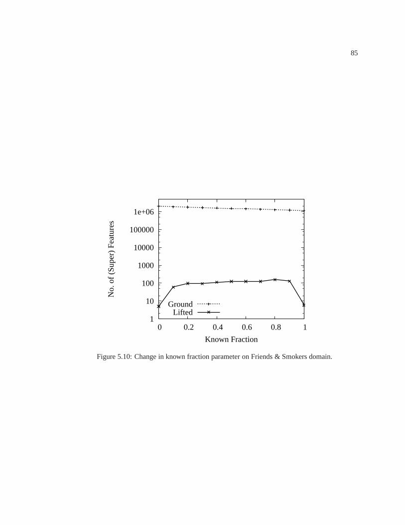
85
1
10
100
1000
10000
100000
1e+06
0 0.2 0.4 0.6 0.8 1
No.
of (
Sup
er)
Fea
ture
s
Known Fraction
GroundLifted
Figure 5.10: Change in known fraction parameter on Friends &Smokers domain.

86
Chapter 6
PARAMETER LEARNING
6.1 Introduction
Learning the parameters of a Markov logic network involves finding the weights that optimize a
likelihood function given the training data. This is a difficult task because computing the likelihood
and its gradient requires performing inference, which has worst-case exponential cost. An oft-used
alternative is to optimize instead a pseudo-likelihood measure, which involves only each variable’s
probability given its Markov blanket (graph neighbors) in the data [2]. This is the approach used
by Richardson and Domingos [86]. However, the pseudo-likelihood ignores non-local interactions
between variables, and may underperform when these need to be taken into account at inference
time.
Both likelihood and pseudo-likelihood are generative learning approaches in the sense that they
attempt to optimize the joint distribution of all variables. In contrast, discriminative approaches
maximize the conditional likelihood of a set of outputs given a set of inputs (e.g., Laffertyet al.[50]).
This often produces better results, because no effort is spent modeling dependencies between inputs.
The voted perceptron is a discriminative algorithm for labeling sequence data, a special case in
which tractable inference is possible using the Viterbi algorithm [12]. In this chapter we generalize
the voted perceptron to arbitrary Markov logic networks, byreplacing the Viterbi algorithm with
a weighted satisfiability solver. Experiments in two real-world domains show the promise of this
approach.
We should point out that since the time of the research described in this chapter, more sophisti-
cated algorithms (some of them based on second-order methods) for discriminatively learning MLN
weights have been proposed. See Lowd and Domingos [59] for details.
We first describe the generative training method. We then describe our algorithm for discrimi-
native learning of MLNs. Finally, we report our experiments.
87
6.2 Generative Training
MLN weights can be learned generatively by maximizing the likelihood of a relational database
(Equation 2.4). (A closed-world assumption is made, whereby all ground atoms not in the database
are assumed false.) The gradient of the log-likelihood withrespect to the weights is
∂
∂wi
log Pw(X =x) = ni(x)−∑
x′
Pw(X =x′) ni(x′) (6.1)
where the sum is over all possible databasesx′, andPw(X =x′) is P (X =x′) computed using the
current weight vectorw = (w1, . . . , wi, . . .). In other words, theith component of the gradient is
simply the difference between the number of true groundingsof the ith formula in the data and its
expectation according to the current model. Unfortunately, computing these expectations requires
inference over the model, which can be very expensive. Most fast numeric optimization methods
(e.g., conjugate gradient with line search, L-BFGS) also require computing the likelihood itself
and hence the partition functionZ, which is also intractable. Although inference can be done
approximately using Markov chain Monte Carlo, Richardson and Domingos [86] found this to be
too slow. Instead, they maximized the pseudo-likelihood ofthe data, an alternative measure widely
used in areas like spatial statistics, social networks and natural language [2]. Ifx is a possible world
(relational database) andxl is thelth ground atom’s truth value, the pseudo-log-likelihood ofx given
weightsw is
log P ∗w(X =x) =
n∑
l=1
log Pw(Xl =xl|MBx(Xl)) (6.2)
whereMBx(Xl) is the state ofXl’s Markov blanket in the data (i.e., the truth values of the ground
atoms it appears in some ground formula with). Computing thepseudo-likelihood and its gradient
does not require inference, and is therefore much faster. However, the pseudo-likelihood parameters
may lead to poor results when inference across non-neighboring variables is required.
6.3 Discriminative Training
In many applications, we knowa priori which predicates will be evidence and which ones will be
queried, and the goal is to correctly predict the latter given the former. If we partition the ground

88
atoms in the domain into a set of evidence atomsX and a set of query atomsY , theconditional
likelihoodof Y givenX is
P (y|x) =1
Zxexp
∑
i∈FY
wini(x, y)
=1
Zx
exp
∑
j∈GY
wjgj(x, y)
(6.3)
whereFY is the set of all MLN clauses with at least one grounding involving a query atom,ni(x, y)
is the number of true groundings of theith clause involving query atoms,GY is the set of ground
clauses inML,C involving query atoms, andgj(x, y) = 1 if the jth ground clause is true in the data
and 0 otherwise. When some variables are “hidden” (i.e., neither query nor evidence) the conditional
likelihood should be computed by summing them out, but for simplicity we treat all non-evidence
variables as query variables. The gradient of the conditional log-likelihood (CLL) is
∂
∂wi
log Pw(y|x) = ni(x, y)−∑
y′
Pw(y′|x)ni(x, y′)
= ni(x, y)− Ew[ni(x, y)] (6.4)
As before, computing the expected countsEw[ni(x, y)] is intractable. However, they can be approx-
imated by the countsni(x, y∗w) in the MAP statey∗w(x). This will be a good approximation if most
of the probability mass ofPw(y|x) is concentrated aroundy∗w(x). Computing the gradient of the
CLL now requires only MAP inference to findy∗w(x), which is much faster than the full conditional
inference forEw[ni(x, y)]. (If the training database is broken up into separate examples, an MAP
inference per example is performed.) This approach was usedsuccessfully by Collins (2002) in
the special case of a Markov network (and hence of an MLN) where the query nodes form a linear
chain. In this case, the MAP state can be found in polynomial time using the Viterbi algorithm, a
form of dynamic programming [85]. Collins’svoted perceptronalgorithm initializes all weights to
zero, performsT iterations of gradient ascent using the approximation above, and returns the pa-
rameters averaged over all iterations,wi =∑T
t=1 wi,t/T . The parameter averaging helps to combat
overfitting.T is chosen using a validation subset of the training data.
89
Generalizing this solution to arbitrary MLNs requires replacing the Viterbi algorithm with a
general-purpose algorithm for MAP inference in MLNs. The form of Equation 6.3 suggests a solu-
tion. Sincey∗w(x) is the state that maximizes the sum of the weights of the satisfied ground clauses,
it can be found using the MaxWalkSat solver (see the section on logic). Given an MLN and set of
evidence atoms, the KB to be passed to MaxWalkSat is formed byconstructing all groundings of
clauses in the MLN involving query atoms, replacing the evidence atoms in those groundings by
their truth values, and simplifying. When hidden variablesare present, the algorithm of Richardson
and Domingos (2006, Table III) is used. (In practice, it is often convenient to make a closed world
assumption on the evidence predicates, whereby all ground predicates not explicitly listed in the
evidence database are assumed false.)
Unlike the Viterbi algorithm, MaxWalkSat is not guaranteedto find the global MAP state. This is
a potential additional source of error in the weight estimates produced. The quality of the estimates
can be improved by running a Gibbs sampler starting at the state returned by MaxWalkSat, and
averaging counts over the samples. If thePw(y|x) distribution has more than one mode, doing
multiple runs of MaxWalkSat followed by Gibbs sampling may also be useful. In the limit, this
is equivalent to computing the expected counts exactly, which gives us a straightforward way of
trading off computational cost and accuracy of estimates.
MaxWalkSat assumes that all weights are positive, while learning can produce negative weights.
However, it is easily shown that a formula with a negative weight in a grounded MLN is equivalent
to its negation with the symmetric weight. We thus perform this conversion, if necessary, before
passing a ground network to MaxWalkSat. The negation of a clause∨n
i=1 Li, whereLi is a literal,
is∧n
i=1 ¬Li, a conjunction ofn unit clauses. If the original clause’s weight isw, we assign a weight
of −w/n to each of these unit clauses.
A step of gradient ascent consists of settingwi,t = wi,t−1+η ∂∂wi
log Pw(y|x)|wt−1. The original
voted perceptron algorithm uses a learning rate ofη = 1. In the generalized version, we have found
it useful to set this value using a validation set, as is typically done. Weights are initialized to the
corresponding clauses’ log odds of being true in the data; this tends to produce faster convergence.
(Because the optimization problem is convex, the initial state does not affect the solution found.)

90
6.4 Experiments
6.4.1 Databases
We carried out experiments on two publicly-available databases: the UW-CSE database used by
Richardson and Domingos [86], and McCallum’s Cora databaseof computer science citations.
The UW-CSE database describes the relationships between professors, students, courses, pub-
lications etc. in the UW computer science department. The dataset has already been described in
detail in Chapter 5. We used the hand-coded knowledge base provided with it, which includes 94 for-
mulas stating various regularities. The query atoms are allgroundings ofAdvisedBy(person1, person2),
and the evidence atoms are all groundings of all other predicates exceptStudent(person) and
Professor(person), corresponding to the “Partial Information” scenario in Richardson and Domin-
gos [86].
The Cora database is a collection of 1295 different citations to computer science research papers.
The details of the dataset have already been described in Chapter 4. We used the hand-coded KB
available with the dataset, consisting of 46 clauses stating various regularities.
6.4.2 Systems
We compared three versions of MLN weight learning, applied to the formulas in the hand-coded KB:
the voted perceptron algorithm with MaxWalkSat inference,as described in the previous section
(MLN(VP)); maximum likelihood using MC-MLE, as described in Richardson and Domingos [86]
(MLN(ML)); and pseudo-likelihood, as described in Richardson and Domingos [86] (MLN(PL)).
In addition, we compared MLN learning with a pure ILP approach (CLAUDIEN [18] (CL)), a
pure knowledge-based approach (the hand-coded KB (KB)), and two pure probabilistic approaches:
naive Bayes (NB) [24] and Bayesian networks (BN) [37].
In MLN(VP) training, we used a single run of MaxWalkSat during each learning iteration. In
the UW-CSE domain we usedη = 0.001 andT = 200. In Cora we usedη = 5 × 10⁻⁷ and
T = 100. (Cora has a much larger number of query predicates than UW-CSE, necessitating the use
of a much smaller learning rate.) Following Richardson and Domingos [86], we trained MLN(PL)
and MLN(ML) using L-BFGS with a zero-centered Gaussian prior. We used Gibbs sampling to
approximate the function value and gradient for MLN(ML). Running it to convergence was found

91
to be too slow for the learning to complete in any practical amount of time. A single inference did
not satisfy the convergence criteria even when run for more than 24 hours. To obtain the estimates
in a reasonable time, we limited each Gibbs sampling inference to at most 50,000 passes for burn-
in and 500,000 passes for mixing. The total learning time waslimited to a maximum of three
days. For inference in all the MLN systems, we used a single run of MaxWalkSat to compute the
MAP truth values of non-evidence atoms, followed by Gibbs sampling to compute their conditional
probabilities given the evidence.
We used the same settings for CLAUDIEN as Richardson and Domingos, and let CLAUDIEN
run for 24 hours on a Sun Blade 1000 workstation.1
In the UW-CSE domain, we used the algorithm of Richardson andDomingos [86] to construct
attributes for the naive Bayes and Bayesian network learners. Following Richardson and Domingos,
we tried using order-1 and order-1+2 attributes, and reportthe best results. In the Cora domain, we
used the evidence predicates as attributes (i.e., we predicted whether two fields values are the same
from their TF-IDF similarity scores; for the citations, evidence values from all the corresponding
fields were used as attributes.).
6.4.3 Methodology
In the UW-CSE domain, we used the same leave-one-area-out methodology as Richardson and
Domingos [86]. In the Cora domain, we performed eight-fold cross-validation, ensuring that no
true set of matching records was split between folds, to avoid train-test set contamination. For
each system on each test set, we measured the conditional log-likelihood (CLL) and area under the
precision-recall curve (AUC) for the query predicate. The advantage of the CLL is that it directly
measures the quality of the probability estimates produced. The advantage of the AUC is that it is
insensitive to the large number of true negatives (i.e., ground atoms that are false and predicted to be
false). The CLL of a query predicate is the average over all its groundings of the ground atom’s log-
probability given the evidence. The precision-recall curve for a predicate is computed by varying
the threshold CLL above which a ground atom is predicted to betrue. We computed the standard
deviations of the AUCs using the method of Richardson and Domingos [86]. To obtain probabilities
1CLAUDIEN only runs on Solaris machines.

92
Table 6.1: Experimental results on the UW-CSE database.
System CLL AUC
MLN(VP) −0.033±0.003 0.295±0.022
MLN(ML) −0.063±0.004 0.077±0.011
MLN(PL) −0.034±0.003 0.232±0.024
KB −0.053±0.004 0.114±0.004
CL −0.693±0.000 0.006±0.000
NB −1.237±0.035 0.065±0.000
BN −0.046±0.002 0.020±0.000
from CL and KB (required to compute CLLs and AUCs) we treated CLAUDIEN’s output and the
hand-coded KBs as MLNs with all equal infinite weights. We smoothed all probabilities for all
systems as in Richardson and Domingos [86].
6.4.4 Results
The results on the UW-CSE domain are shown in Table 6.1. MLNs with discriminative training
clearly outperform all the other approaches. The poor results of MLN(ML) are attributable to the
fact that learning using non-converged chains of Gibbs sampling produces parameters which are far
from optimal. MLN(PL) is only marginally worse than MLN(VP)on CLL but loses substantially
on AUC. Purely logical and purely probabilistic approachesall give poor results.
The results on Cora are shown in Tables 6.2 and 6.3. Again, MLNs with discriminative training
outperform the other approaches. The performance of MLN(ML) is very poor due to the non-
convergence of Gibbs sampling. MLN(PL) performs much worsethan MLN(VP) on both CLL and
AUC. The purely logical KB performs very poorly. CL performsbetter than KB, but still much
worse than MLN(VP). Among the probabilistic approaches, BNperforms marginally better than
MLN(VP) on CLL on predicting citations, but significantly worse on AUC. On authors and venues,
MLN(VP) outperforms all other approaches on both CLL and AUC.

93
Table 6.2: CLL results on the Cora database.
System Citation Author Venue
MLN(VP) −0.069±0.001 −0.069±0.008 −0.232±0.006
MLN(ML) −13.26±0.013 −12.97±0.086 −13.38±0.034
MLN(PL) −0.699±0.000 −3.062±0.046 −0.708±0.002
KB −8.629±0.009 −8.096±0.062 −8.475±0.022
CL −0.461±0.000 −2.375±0.069 −1.261±0.022
NB −0.082±0.000 −0.203±0.008 −0.233±0.003
BN −0.067±0.000 −0.203±0.008 −0.233±0.003
6.5 Conclusion
In this chapter, we presented an algorithm for discriminative learning of MLN parameters. The
algorithm is based on the voted perceptron algorithm proposed by Collins for learning HMMs. We
generalized it to Markov logic, replacing Viterbi in the Collins algorithm by a weighted satisfiability
solver. Our experiments show that this approach outperforms generative learning.

94
Table 6.3: AUC results on the Cora database.
System Citation Author Venue
MLN(VP) 0.973±0.000 0.969±0.001 0.771±0.003
MLN(ML) 0.111±0.000 0.162±0.000 0.061±0.000
MLN(PL) 0.722±0.001 0.323±0.001 0.342±0.005
KB 0.149±0.000 0.180±0.000 0.096±0.000
CL 0.187±0.000 0.090±0.000 0.047±0.000
NB 0.945±0.000 0.734±0.006 0.339±0.001
BN 0.951±0.000 0.734±0.006 0.339±0.001

95
Chapter 7
A UNIFIED APPROACH TO ENTITY RESOLUTION
7.1 Introduction
In this chapter and the next, we will describe applications of Markov logic to two important real
world problems. The first one, described in this chapter, is the problem of entity resolution. The next
chapter describes the application of Markov logic to the problem of identifying social relationships
in image collections.
Entity resolution is the problem of identifying which of thereferences in a given dataset refer
to the same underlying entity or object in the real world. These are records that, while not syn-
tactically identical, represent the same real-world entity. For instance, given a citation database,
we may be interested in identifying the references that refer to the same underlying paper. These
references, though referring to the same paper, may differ from each other, because of variations
in the way authors names are written, conference names beingabbreviated, spelling mistakes and
so on. This problem is known by the name of entity resolution,record linkage, object identifica-
tion, de-duplication, merge/purge, data association, identity uncertainty, reference reconciliation,
and others.
The problem of entity resolution often occurs in the processof data cleaning and preparation
which is the first stage in the data mining process, and in mostcases it is by far the most expensive.
Data from relevant sources must be collected, integrated, scrubbed and pre-processed in a variety of
ways before accurate models can be mined from it. When data from multiple databases is merged
into a single database, many duplicate records often result. Correctly merging these records and
the information they represent is an essential step in producing data of sufficient quality for mining.
In recent years this problem has received growing attentionin the data mining community, with a
related workshop at KDD-2003 [62] and a related task as part of the 2003 KDD Cup [29].
The entity resolution problem was first identified by Newcombe et al. [72], and given a statistical
formulation by Fellegi and Sunter [26]. Most current approaches are variants of the Fellegi-Sunter

96
model, in which entity resolution is viewed as a classification problem: given a vector of similarity
scores between the attributes of two entities, classify it as “Match” or “Non-match.” A separate
match decision is made for each candidate pair, followed by transitive closure to eliminate incon-
sistencies. Typically, a logistic regression model is used[1]. One line of research has focused on
scaling entity resolution to large databases by avoiding the quadratic number of comparisons be-
tween all pairs of entities (e.g., [38, 67, 61, 11]). Anotherhas focused on the use of active learning
techniques to minimize the need for labeled data (e.g., [100, 89, 5]). Several authors have devised,
compared and learned similarity measures for use in entity resolution (e.g., [10, 101, 4]). A number
of alternate formulations have also been proposed (e.g., [9]). Entity resolution has been applied in a
wide variety of domains (e.g., [74, 17]) and to different types of data, including text (e.g., [55]) and
images (e.g., [40]). Winkler [105] surveys research in traditional record linkage.
Most recently, several authors have pointed out that match decisions should not be made in-
dependently for each candidate pair. While the Fellegi-Sunter model treats all pairs of candidate
matches as i.i.d. (independent and identically distributed), this is clearly not the case, since each
entity appears in multiple candidate matches. While this interdependency complicates learning and
inference, it also offers the opportunity to improve entityresolution, by taking into account infor-
mation that was previously ignored. For example, Singla andDomingos [94], Donget al. [25] and
Culotta and McCallum [14] allow the resolution of entities of one type to be helped by resolution
of entities of related types (e.g., if two papers are the same, their authors are the same, which in
turn is evidence that other pairs of papers by the same authors should be matched, etc.). McCallum
and Wellner [63] incorporate the transitive closure step into the statistical model. Pasulaet al. [76]
incorporate parsing of entities from citation lists into a citation matching model. Bhattacharya and
Getoor [3] use coauthorship relations to help match authorsin citation databases. Milchet al. [66]
propose a language for reasoning about entity resolution. Shenet al. [92] exploit various types
of constraints to improve matching accuracy. Daviset al. [17] use inductive logic programming
techniques to discover relational rules for entity resolution, which they then combine using a naive
Bayes classifier.
One of the key problems with the approaches described above is that they address isolated as-
pects of the problem, e.g., transitivity. Further, most of them have been developed as standalone
systems, which makes it difficult to compare and combine themwith other approaches. Incorpo-

97
rating any new approaches is even more difficult. What is desirable is a unified approach, which is
easy to understand and allows us to combine the benefits of various approaches into a single model.
In this chapter we propose a simple and mathematically soundformulation of the entity reso-
lution problem based on Markov logic that incorporates the non-i.i.d. approaches described above,
and can be viewed as a generalization of the Fellegi-Sunter model. Our model can seamlessly com-
bine many different approaches by writing a few weighted formulas in Markov logic for each. This
allows us to readily use the existing machinery of Markov logic for performing efficient learning
and inference. We illustrate this by combining a few salientapproaches to entity resolution, and ap-
plying the resulting system to a large citation database. Wewill first describe our proposed approach
to entity resolution, followed by our experiments.
7.2 MLNs for Entity Resolution
7.2.1 Equality in Markov Logic
Most systems for inference in first-order logic make theunique names assumption: different con-
stants refer to different objects in the domain. This assumption can be removed by introducing the
equality predicate(Equals(x, y) or x = y for short) and its axioms [30]:
Reflexivity: ∀x x = x.
Symmetry: ∀x, y x = y ⇒ y = x.
Transitivity: ∀x, y, z x = y ∧ y = z ⇒ x = z.
Predicate equivalence:For each binary predicateR:
∀x1, x2, y1, y2 x1 = x2 ∧ y1 = y2 ⇒ (R(x1, y1) ⇔ R(x2, y2)). Similar axioms are re-
quired for predicates of other arities and for functions, but binary predicates suffice for this
dissertation.
Adding the formulas above with infinite weight to an MLN allows it to handle non-unique
names. We can also add the reverse of the last one with finite weight:

98
Reverse predicate equivalence:For each binary predicateR: ∀x1, x2, y1, y2 R(x1, y1)∧R(x2, y2)⇒
(x1 = x2 ⇔ y1 = y2), and similarly for other arities and functions.
The meaning of this formula is most easily understood by noting that it is equivalent to the two
clauses:
∀x1, x2, y1, y2 R(x1, y1) ∧R(x2, y2) ∧ x1 = x2 ⇒ y1 = y2
∀x1, x2, y1, y2 R(x1, y1) ∧R(x2, y2) ∧ y1 = y2 ⇒ x1 = x2
As statements in first-order logic, these clauses are false,because different groundings of the
same predicate do not generally represent the same tuples ofobjects. However, when added to an
MLN with a finite weight, they capture an important statistical regularity: if two objects are in the
same relation to the same object, this is evidence that they may be the same object. Some rela-
tions provide stronger evidence than others, and this is captured by assigning (or learning) different
weights to the formula for differentR. For example, when de-duplicating citations, two papers
having the same title is stronger evidence that they are the same paper than them having the same
author, which in turn is stronger evidence than them having the same venue. However, even the
latter is quite useful: two papers appearing in the same venue are much more likely to be the same
than two papers about which nothing is known.
Remarkably,the equality axioms and reverse predicate equivalence are all that is needed to
perform entity resolution in Markov logic. As we will see, despite its simplicity, this formulation
incorporates the essential features of some of the most sophisticated entity resolution approaches to
date, including the “collective inference” approaches of McCallum and Wellner [63] and Singla and
Domingos [94]. A number of other approaches can be incorporated by adding the corresponding
formulas. (We emphasize that our goal is not to reproduce every detail of these approaches, but
rather to capture their essential features in a simple, consistent form.) Further, entity resolution and
data mining can be seamlessly combined, and aid each other, by performing structure learning on
top of the entity resolution MLN.

99
7.2.2 Problem Formulation
We now describe our proposed approach in detail. For simplicity, we assume that the database to
be deduplicated contains only binary relations. This entails no loss of generality, because ann-
ary relation can always be re-expressed asn binary relations. For example, if a citation database
contains ground atoms of the formPaper(title, author, venue), they can be replaced by atoms of
the formHasTitle(paper, title), HasAuthor(paper, author) andHasVenue(paper, venue).
Each real-world entity (e.g., each paper, author or venue) is represented by one or more strings
appearing as arguments of ground atoms in the database. For example, different atoms could contain
the stringsICDM-2006, Sixth ICDM andIEEE ICDM’06, all of which represent the same conference.
We assume that the predicates in the database (representingrelations in the real world) aretyped;
for example, the first argument of the predicateHasAuthor(paper, author) is of typePaper, and
the second is of typeAuthor. The goal of entity resolution is, for each pair of constantsof the
same type(x1, x2), to determine whether they represent the same entity: isx1 = x2? Thus the
query predicate for inference is equality; the evidence predicates are the (binarized) relations in the
database, and other relations that can be deterministically derived from the database (see below).
The model we use for entity resolution is in the form of an MLN,with formulas and weights that
may be hand-coded and/or learned. The most likely truth assignment to the query atoms given
the evidence is computed using MaxWalkSAT. Conditional probabilities of query atoms given the
evidence are calculated using Gibbs sampling.
The model includes a unit clause for each query predicate. (Aunit clause is a clause containing
only one literal.) The weight of a unit clause captures (roughly speaking) the marginal distribution
of the corresponding predicate, leaving non-unit clauses to capture the dependencies between pred-
icates. Since most groundings of most predicates are usually false (e.g., most pairs of author strings
do not represent the same author), it is clearest to use unit clauses consisting of negative literals, with
positive weights. Since predicate arguments are typed, there is a unit clause for equality between
entities of each type (e.g.,paper1 = paper2, author1 = author2, etc.). From a discrimina-
tive point of view, the weight of a unit clause represents thethreshold above which evidence must
accumulate for a candidate pair of the corresponding type tobe declared a match.

100
7.2.3 Field Comparison
We assume that each field in a database to be deduplicated is a string composed of one or more
words (or, more generally, tokens), and define the predicateHasWord(field, word) which is true
iff field containsword. Applied to this predicate, reverse predicate equivalencestates that
∀x1, x2, y1, y2 HasWord(x1, y1) ∧ HasWord(x2, y2) ∧ y1 = y2 ⇒ x1 = x2
or, in other words, fields that have a word in common are more likely to be the same. When
inserted into Equation 2.4, and assuming for the moment no other clauses, this clause produces a
logistic regression for the field match predicatex1 = x2 as a function of the number of wordsn
the two fields have in common:P (x1 = x2 | n) = 1/(1 + e−wn), wherew is the weight of the
formula. Effectively, then, reverse predicate equivalence applied toHasWord() implements a simple
similarity measure between fields. This measure can be made adaptive, in the style of Bilenko and
Mooney [4], by learning a different weight for each grounding of reverse predicate equivalence with
a different word. (Groundings wherey1 6= y2 are always satisfied, and therefore their weights cancel
out in the numerator and denominator of Equation 2.4, and areirrelevant. Reflexivity ensures the
proper treatment of groundings wherey1 = y2.)
It can also be useful to add the “negative” version of reversepredicate equivalence:
∀x1, x2, y1, y2 ¬HasWord(x1, y1) ∧ HasWord(x2, y2) ∧ y1 = y2 ⇒ x1 6= x2
∀x1, x2, y1, y2 HasWord(x1, y1) ∧ ¬HasWord(x2, y2) ∧ y1 = y2 ⇒ x1 6= x2
∀x1, x2, y1, y2 ¬HasWord(x1, y1) ∧ ¬HasWord(x2, y2) ∧ y1 = y2 ⇒ x1 = x2
Like other word-based similarity measures, this approach has the disadvantage that it treats mis-
spellings, variant spellings and abbreviations of a word ascompletely different words. Since these
are often a significant issue in entity resolution, it would be desirable to account for them. One
way to do this efficiently is to compare word strings by the engrams they contain [36]. This can
be done in our framework by defining the predicateHasEngram(word, engram), which is true iff
engram is a substring ofword. (This predicate can be computed on the fly from its arguments, or
pre-computed for all relevant word-engram pairs and given as evidence.) Applying reverse predicate

101
equivalence to this predicate results in a logistic regression model for the equality of two words as
a function of the number of engrams they have in common. Combined with the logistic regression
for field equality, this produces a two-level similarity measure, comparing fields as sets of words,
which are in turn compared as strings. Cohenet al. [10] found such hybrid measures to outper-
form pure word-based and pure string-based ones for entity resolution. The maximum length of
engrams to consider is a parameter of the problem. Linear-interpolation smoothing is obtained by
defining different predicates for engrams of different length, with the corresponding weights for the
corresponding versions of reverse predicate equivalence.(These can also be learned, using weight
priors to avoid overfitting.) It is also possible to incorporate string edit distances like Levenshtein
and Needleman-Wunsch [4] into an MLN. This involves statingformulas analogous to the recur-
rence relations used to compute these distances, with (negative) weights corresponding to the costs
of insertion, deletion, etc. Pursuing this approach is an item for future work.
7.2.4 The Fellegi-Sunter Model
The Fellegi-Sunter model uses naive Bayes to predict whether two records are the same, with field
comparisons as the predictors [26]. If the predictors are the field match predicates, Fellegi-Sunter is
a special case of reverse predicate equality, withR as the relation between a field and the record it
appears in (e.g.,HasAuthor(paper, author)). If the predictors are field similarities, measured by
the number of words present in both, either and none of the fields, Fellegi-Sunter is implemented by
clauses of the form
∀x1, x2, y1, y2 HasWord(x1, y1) ∧ HasWord(x2, y2) ∧ y1 = y2 ∧R(z1, x1) ∧R(z2, x2)
⇒ z1 = z2
∀x1, x2, y1, y2 ¬HasWord(x1, y1) ∧ HasWord(x2, y2) ∧ y1 = y2 ∧R(z1, x1) ∧R(z2, x2)
⇒ z1 6= z2
∀x1, x2, y1, y2 HasWord(x1, y1) ∧ ¬HasWord(x2, y2) ∧ y1 = y2 ∧R(z1, x1) ∧R(z2, x2)
⇒ z1 6= z2
∀x1, x2, y1, y2 ¬HasWord(x1, y1) ∧ ¬HasWord(x2, y2) ∧ y1 = y2 ∧R(z1, x1) ∧R(z2, x2)
⇒ z1 = z2

102
∀z1, z2 z1 6= z2
for each field-record relationR. The last rule corresponds to the class priors implemented as a unit
clause.
7.2.5 Relational Models
The combination of Fellegi-Sunter with transitivity produces McCallum and Wellner’s [63] condi-
tional random field (CRF) model, with field matches or field similarities as the features. (A logistic
regression model is a CRF where all the query variables are independent; transitive closure renders
them dependent. Discriminatively-trained MLNs can be viewed as relational extensions of CRFs.)
Reverse predicate equivalence applied to the relations in the database yields the CRF model of
Singla and Domingos [94], with the field similarity measure described above instead of TF-IDF. It
is also very similar to the CRF model of Culotta and McCallum [14]. The model of Donget al. [25]
is also of this type, but moread hoc. All of these models have the property that they allow entities
of multiple types to be resolved simultaneously, with inference about one pair of entities triggering
inferences about related pairs of entities (e.g., if two papers are the same, their authors are the same;
and vice-versa, albeit with lower weight).
We can also use coauthorship relations for entity resolution, in the vein of Bhattacharya and
Getoor [3], by defining theCoauthor(x1, x2) predicate using the formula
∀x, y1, y2 HasAuthor(x, y1) ∧ HasAuthor(x, y2)⇒ Coauthor(y1, y2)
with infinite weight, and applying reverse predicate equivalence to it. (We can also explicitly state
that coauthorship is reflexive and symmetric, but this is notnecessary.) Notice that this approach
increases the likelihood that two authors are the same even if they are coauthors of a third author on
differentpapers. While this is still potentially useful, a presumably stronger regularity is captured
by the clause
∀x1, x2, y1, y2, y3, y4 HasAuthor(x1, y1) ∧ HasAuthor(x2, y2) ∧ HasAuthor(x1, y3)
∧ HasAuthor(x2, y4) ∧ x1 = x2 ∧ y1 = y2 ⇒ y3 = y4.

103
This formula is related to reverse predicate equivalence, but (with suitably high weight) represents
the non-linear increase in evidence that can occur when boththe papers and the coauthors are the
same.
So far, we have seen that an MLN with a small number of hand-coded formulas representing
properties of equality is sufficient to perform state-of-the-art entity resolution. However, one of the
key features of the entity resolution problem is that a wide variety of knowledge, much of it domain-
dependent, can (and needs to) be brought to bear on matching decisions. This knowledge can be
incorporated into our approach by expressing it in first-order logic. For example, the constraints
listed by Shenet al. [92] can all be incorporated into an MLN in this way. Weightedsatisfiability
then performs the role of relaxation labeling in Shen at al. It is also possible to incorporate formulas
learned independently using ILP techniques, as in Daviset al. [17], or to refine the hand-coded
formulas and construct additional ones using MLN structurelearning [47].
7.2.6 Scalability
In practice, even for fairly small databases there will be a large number of equality atoms to infer
(e.g., 1000 constants of one type yield a million equality atoms). However, the vast majority of
these will usually be false (i.e., non-matches). Scalability is typically achieved by performing infer-
ence only over plausible candidate pairs, identified using acheap similarity measure (e.g., TF-IDF
computed using a reverse index from words to fields). This approach can easily be incorporated
into our framework simply by adding all the non-plausible matches to the evidence as false atoms.
Most clauses involving these atoms will always be satisfied,and thus there is no need to ground
them. We select plausible candidates using McCallumet al.’s canopy approach [61], with TF-IDF
cosine as the similarity measure, but any other approach could be used. While some of the apparent
non-matches might be incorrect, this is a necessary and veryreasonable approximation. Notice that
reverse predicate equivalence might be able to correct someof these errors, by indirectly inferring
that two very different strings in fact represent the same object. We have developed a version of
MaxWalkSAT and MCMC that lazily grounds predicates and clauses, effectively allowing predi-
cates that are initially assumed false to be revisited, without incurring the computational cost of
completely grounding the network (see Chapter 4). Incorporating this into our entity resolution

104
system is an item for future work.
7.3 Experiments
7.3.1 Datasets
We used two publicly available citation databases in our experiments: Cora and BibServ. These
datasets have already been described in previous chapters,but for the sake of completeness of this
chapter, we will mention some of the important details again.
Cora
Cora dataset is a collection of 1295 different citations to computer science research papers from
the Cora Computer Science Research Paper Engine. We used theversion processed by Bilenko and
Mooney [4] where each citation was segmented into fields (author, venue, title, publisher, year, etc.)
using an information extraction system. We used this processed version of Cora. We further cleaned
it up by correcting some labels. This cleaned version contains references to 132 different research
papers. We used only the three most informative fields: first author, title and venue (with venue
including conferences, journals, workshops, etc.). We compared the performance of the algorithms
for the task of de-duplicating citations, authors and venues. For training and testing purposes, we
hand-labeled the field pairs. The labeled data contains references to 50 authors and 103 venues.
After forming canopies, the total number of match decisionswas 61,177.
BibServ
BibServ.org is a publicly available repository of about half a million pre-segmented citations. It is
the result of merging citation databases donated by its users, CiteSeer, and DBLP. We experimented
on a subset of 10,000 records extracted randomly from the user-donated subset of BibServ, which
contains 21,805 citations. As in Cora, we used the first author, title and venue fields. In order to
focus only on hard decisions, we discarded all the canopies of size less than 10. This left us with a
total of 15,954 decisions. Since we lacked labeled data for BibServ, we used the parameters learned
on Cora (with appropriate modifications) to perform inference on BibServ. Word stemming was
used to identify the variations of the same underlying root word both in Cora and BibServ.

105
7.3.2 Models
We compared the following models in our experiments.
NB. This is the naive Bayes model as described in Section 7.2.4. We use a different feature for
every word.
MLN(B). This is the basic MLN model closest to naive Bayes. Ithas the four reverse predicate
equivalence rules connecting each word to the corresponding field/record match predicate.
With per-word weights, this yields thousands of weights. For speed, these are derived from
the naive Bayes parameters. The model also has a unit clause,¬SameEntity(e1, e2), for
each entity type being matched. The weights of these rules are learned discriminatively using
the algorithm of Singla and Domingos [93]. When the weights of single predicate rules are
set using the class priors in naive Bayes, the two models are equivalent. All the following
models are obtained by adding specific rules to the basic MLN model and learning these rules
discriminatively.
MLN(B+C). This is obtained by adding reverse predicate equivalence rules for the various fields to
MLN(B). This achieves the flow of information through sharedattribute values as proposed
by Singla and Domingos [94].
MLN(B+T). This is obtained by adding transitive closure rules to MLN(B). It incorporates transi-
tivity into the model itself as proposed by McCallum and Wellner [63].
MLN(B+C+T). This model has both reverse predicate equivalence and transitive closure rules and
i.e. it has the enhancements proposed by both Singla and Domingos [94] and McCallum and
Wellner [63].
MLN(B+C+T+S). This model is obtained by adding rules learned using the structure learning algo-
rithm of Kok and Domingos [47] to MLN(B+C+T). An example of a rule added by structure
learning is: if two papers have the same title and the same venue, then they are the same paper.

106
MLN(B+N+C+T). This model has a two-level learning/inference step. The first step involves
learning a model to predict if two word mentions are the same based on then-grams they
have in common (we usedn=3). This step incorporates word-level transitivity and reverse
predicate equivalence rules. The second step involves learning an MLN(B+C+T) model on
the words inferred by the first stage.1 This model implements a hybrid similarity measure as
proposed by Cohenet al. [10].
MLN(G+C+T). This model is similar to MLN(B+C+T) except thatit does not have per-word
reverse predicate equivalence rules. Rather, it has four global rules, each with the same weight
for all words, and these weights are learned discriminatively, like the rest.2
7.3.3 Methodology
In the Cora domain, we performed five-fold cross validation.In the BibServ domain, because of the
absence of labeled data, the naive Bayes model could not be learned. The weights of the inverse
predicate equivalence rules for each word were fixed in proportion to the IDF of the word. This was
used as a baseline for all the enhanced models. The weights ofother rules were determined from
the weights learned on Cora for the corresponding model.
For each model, we measured the conditional log-likelihood(CLL) and area under the precision-
recall curve (AUC) for the match predicates. The advantage of the CLL is that it directly measures
the quality of the probability estimates produced. The advantage of the AUC is that it is insensitive
to the large number of true negatives (i.e., ground atoms that are false and predicted to be false).
The CLL of a set of predicates is the average over all their groundings of the ground atom’s log-
probability given the evidence. The precision-recall curve for match predicates is computed by
varying the threshold CLL above which a ground atom is predicted to be true. We computed the
standard deviations of the AUCs using the method of Richardson and Domingos [86].
1This model was learned on raw words without any stemming, to see if the n-gram step could potentially achieve theeffects of stemming.
2The rule¬HasWord() ∧ ¬HasWord() ⇒ SameField() has essentially no predictive power; we set its weight to 0.

107
7.3.4 Results
Cora
Tables 7.1 and 7.2 show the CLL and AUC for the various models on the Cora dataset, respectively.
For the case of AUC in venues, there is monotonic increase in the performance as we add various
collective inference features to the model, with the best-performing model being MLN(B+C+T).
This trend shows how adding each feature in turn enhances theperformance, giving the largest
improvement when all the features are added to the model. Forthe case of CLL in venues, the per-
formance tends to fluctuate as we add various collective inference features, but the best-performing
model is still MLN(B+C+T). For the case of citations, the results are similar, although the improve-
ments as we add features are not as consistent as in case of AUCin venues. For AUC in authors,
we have similar results, although the performance gain is much smaller compared to venues and
citations. There is more fluctuation in the case of CLL but thecollective models are still the best.
MLN(B+C+T+S) helps improve the performance of MLN(B+C+T) on citations and authors
(both CLL and AUC) but does not help on venues.
MLN(B+N+C+T) improves performance on authors but not on citations and venues. This shows
that while stemming can be a good way of identifying word duplicates in most cases, the engram
model is quite helpful when dealing with fields such as authors, where initials are used for the
complete word and can not be discovered by stemming alone.
MLN(G+C+T) (the model with global word rules) performs wellfor citations but less so for
authors and venues. In general, per-word rule models seem tobe particularly helpful when there are
few words from which to infer the relationship between two entities.
BibServ
Since we did not have labeled data for BibServ, we hand-labeled 300 pairs each for citations and
venues, randomly selected from the set where the MAP prediction for at least one of the algorithms
was different from the others. For authors, we labeled all the potential match decisions, as there
were only 240 of them. The results reported below are over these hand-labeled pairs.
Tables 7.3 and 7.4 show the CLL and AUC for the various algorithms on the BibServ dataset.
As in the case of Cora, for citations and authors, the best-performing models are the ones involving

108
Table 7.1: CLL results on the Cora database.
System Citation Author Venue
NB −0.637±0.010 −0.133±0.021 −0.747±0.017
MLN (B) −0.643±0.010 −0.131±0.022 −0.760±0.017
MLN (B+C) −0.809±0.012 −0.386±0.064 −1.163±0.034
MLN (B+T) −0.369±0.003 −0.213±0.036 −1.036±0.029
MLN (B+C+T) −0.597±0.007 −0.171±0.043 −0.704±0.023
MLN (B+C+T+S) −0.503±0.006 −0.100±0.033 −0.874±0.027
MLN (B+N+C+T) −0.879±0.008 −0.096±0.032 −0.781±0.023
MLN (G+C+T) −0.394±0.004 −0.263±0.053 −1.196±0.031
collective inference features. MLN(B+N+C+T) gives the best performance for both CLL and AUC
in authors, for the reasons cited before. It is also the best-performing model for AUC in citations,
closely followed by other collective models. MLN(B+C) gives the best performance for CLL in
citations.
Whereas MLN(G+C+T) performs quite poorly on citations and authors, it in fact gives the best
performance on CLL in venues. On AUC in venues, MLN(G+C+T) and MLN(B) are the two best
performers. Overall, even though BibServ and Cora have quite different characteristics, applying
the parameters learned on Cora to BibServ still gives good results. Collective inference is clearly
useful, except for AUC on venues, where the results are inconclusive.
7.4 Conclusion
In this chapter, we proposed a unifying framework for entityresolution. We showed how a small
number of axioms in Markov logic capture the essential features of many different approaches to
this problem, in particular non-i.i.d. ones, as well as the original Fellegi-Sunter model. Experiments
on two citation databases evaluate the contributions of these approaches, and illustrate how Markov
logic enables us to easily build a sophisticated entity resolution system.

109
Table 7.2: AUC results on the Cora database.
System Citation Author Venue
NB 0.913±0.000 0.986±0.000 0.738±0.002
MLN (B) 0.915±0.000 0.987±0.000 0.736±0.002
MLN (B+C) 0.891±0.000 0.968±0.000 0.741±0.001
MLN (B+T) 0.949±0.000 0.994±0.000 0.745±0.002
MLN (B+C+T) 0.964±0.000 0.984±0.000 0.828±0.002
MLN (B+C+T+S) 0.988±0.000 0.992±0.000 0.807±0.002
MLN (B+N+C+T) 0.952±0.000 0.992±0.000 0.817±0.002
MLN (G+C+T) 0.973±0.000 0.980±0.000 0.743±0.002
Table 7.3: CLL results on the Bibserv database.
System Citation Author Venue
MLN(B) −0.008±0.003 −0.586±0.114 −0.806±0.121
MLN(B+C) −0.001±0.000 −0.544±0.113 −1.166±0.151
MLN(B+T) −0.006±0.003 −0.600±0.116 −0.827±0.123
MLN(B+C+T) −0.006±0.004 −0.473±0.105 −1.146±0.149
MLN(B+C+T+S) −0.006±0.004 −0.486±0.107 −1.133±0.148
MLN(B+N+C+T) −0.018±0.005 −0.363±0.091 −0.936±0.133
MLN(G+C+T) −0.735±0.101 −4.679±0.256 −0.716±0.112

110
Table 7.4: AUC results on the Bibserv database.
System Citation Author Venue
MLN(B) 0.997±0.001 0.910±0.013 0.908±0.011
MLN(B+C) 0.999±0.000 0.887±0.007 0.876±0.012
MLN(B+T) 0.993±0.003 0.909±0.013 0.898±0.010
MLN(B+C+T) 0.998±0.000 0.928±0.009 0.876±0.012
MLN(B+C+T+S) 0.970±0.020 0.926±0.010 0.876±0.012
MLN(B+N+C+T) 1.000±0.000 0.940±0.008 0.897±0.012
MLN(G+C+T) 0.491±0.000 0.432±0.001 0.906±0.012

111
Chapter 8
DISCOVERY OF SOCIAL RELATIONSHIPS IN IMAGE COLLECTIONS
8.1 Introduction
This chapter describes the application of Markov logic to the problem of identifying social relation-
ships in image collections pertaining to everyday users. Image collections are pervasive. Mining
semantically meaningful information from such collections has been an area of active research in
the machine learning and vision communities. There is a large body of work focusing on problems
of face detection and recognition, detecting objects of certain types such as grass, water, and sky.
Most of this work relies on using low-level features available in the image (such as color or texture).
In recent years, there has been an increased focus on extracting semantically more complex infor-
mation such as scene detection and activity recognition [56, 54]. For example, one might want to
cluster pictures based on whether they were taken outdoors or indoors or cluster work pictures vs.
leisure pictures. This work relies primarily on using the derived features, such as people present in
the image, the presence or absence of certain kinds of objects in the image, and so on. Typically,
the power of collective inference is used in such scenarios [60]. For example, it may be hard to tell
for a particular picture if it is work or leisure, but by looking at other pictures that are similar in
a spatio-temporal sense it becomes easier to arrive at the correct conclusion. This line of research
aims to change the way we perceive digital image collections- from sets of pixels to highly complex
objects that can be organized and queried in meaningful ways.
Our goal is to automatically detect social relationships inimage collections. For example, given
two faces appearing in an image, we would like to infer if the two people are spouses or merely
friends. Even when information about age, gender, and identity of various faces is known, this
task seems extremely difficult. In related work [70, 28], theintention is to learn the likelihood that
particular groups will appear together in images to facilitate recognition. In Wenget al. [104],
movies are analyzed to find groups of associated characters.In all of these works, the relationships
within the groups are left undefined.

112
Given a single image of two people, it is difficult to determine whether the two are friends or
spouses. However, when a group of pictures are considered collectively, the task becomes more
tractable. An observer unfamiliar with the images’ subjects might guess based on heuristic rules
such as (a) couples often tend to appear together in images just by themselves as opposed to friends
who typically appear in groups, and (b) couples with young children often appear with their children
in the images. The power of this approach is that one can even make meaningful inferences even
about relationships between people who never (or very rarely) appear together in an image. For
example, if A (male) appears with a child in a group of images and B (female) appears with the
same child in other images, and A and B appear together in a fewother images, then is it likely they
are spouses and are the child’s parents.
Markov logic allows us to capture these heuristic rules (possibly incorrect and conflicting in
many scenarios) in a mathematically sound and meaningful way. Each rule is seen as a soft con-
straint (as opposed to a hard constraint in logic) whose importance is determined by the real-valued
weight associated with it. These weights are learned from hand-labeled training data. We also
propose to learn new rules using the data, in addition to the rules supplied by the domain experts,
thereby enhancing the background knowledge. These rules (and their weights) are then used to per-
form a collective inference over the set of possible relationships. As we will show, we can also build
a model for predicting relationships, age and gender, usingnoisy predictors (for age and gender)
as inputs to the system. Inference is performed over all images, age, and gender simultaneously to
allow each component to influence the others in the context ofour model, thereby improving the
accuracy of the prediction. We will first describe our model for predicting the social relationships
in image collections, followed by our experimental evaluation.
8.2 Model
Our model is expressed in Markov logic. We will describe our objects of interest, predicates (prop-
erties of objects and relationships among them), and the rules that impose certain constraints on
those predicates. We will then pose our learning and inference tasks.

113
8.2.1 Objects and Predicates
Objects
We have three kinds of objects in our domain:
• Person: A real person in the world.
• Face: A specific appearance of a face in an image.
• Image: An image in the collection.
We model two kinds of predicates defined over the objects of interest.
Evidence Predicates
The value of these predicates is known from the data at the time of the inference. An example
evidence predicate isOccursIn(face, img), which represents the truth value of whether a partic-
ular face appears in a given image or not. We use evidence predicates for the following proper-
ties/relations:
• Number of people in an image:HasCount(img, cnt)
• The age of a face appearing in an image:HasAge(face, age)
• The gender of a face appearing in an image:HasGender(face, gender)
• Whether a particular face appears in an image:OccursIn(face, img)
• Correspondence between a person and his/her face:HasFace(person, face)
The age (gender) of a face is the estimated age (gender) valueestimated from the face from an
image. Note that this is distinct from the actual age (gender) of a person, which is modeled as a
query predicate. The age (gender) associated with a face is inferred from a classification model
trained separately on a collection of faces using various facial features. We implemented age and
gender classifiers following the examples of Li and Fei-Fei [51] and Yedidiaet al. [107]. Note that

114
different faces associated with the same person will likelyhave different estimated age and gender
values. We model the age using five discrete bins: child, teen, youth, adult, and senior.
For this application, we assume the presence of face detection and recognition and therefore we
know exactly which face corresponds to which person. Relaxing this assumption and folding face
detection and recognition into the model is an important direction for future work.
Query Predicates
The value of these predicates is not known at the time of the inference and needs to be inferred. An
example of this kind of predicate isHasRelation(person1, person2, relation), which repre-
sents the truth value of whether two persons share a given relationship. We use the following query
predicates:
• The relationship between two persons:HasRelation(person1, person2, relation)
• Age of a person:PersonHasAge(person, age)
• Gender of a person:PersonHasGender(person, gender)
We model two different kinds of settings.
Two-Class: In this basic setting, we model only two relationships in thedomain: friend or relative.
All the relations are mapped onto one of these two relationships. Relative follows the intuitive defi-
nition of being a relative. Anyone who is not a relative is considered as a friend.
Multi-Class: In the second setting, we model seven different kinds of social relationships: relative,
friend, acquaintance, child, parent, spouse, and childfriend. Relative includes any relative (by blood
or marriage) not including child, parent, or spouse. Friends are people who are not relatives and
satisfy the intuitive definition of friendship. Childfriend models the friends of children. It is impor-
tant to model the childfriend relationship, as children arepervasive in image collections and often
appear with their friends. In such scenarios, it becomes important to distinguish between children
and their friends. Any non-relatives, non-friends are acquaintances. For our purposes and in our
data, spouses always have opposite gender.

115
8.2.2 Rules
We formulate two kinds of rules for our problem. All the rulesare expressed as formulas in first-
order logic.
Hard Rules
These describe the hard constraints in the domain, i.e., they should always hold true. An example of
a hard rule isOccursIn(face, img1)∧ OccursIn(face, img2)⇒ (img1 = img2), which simply
states that each face occurs in at most one image in the collection. Here are some of the other hard
rules that we use:
• Parents are older than their children.
• Spouses have opposite gender.
• Two people have a unique relationship between them.
Note that we assume there is a unique relationship between two people. Relaxing this assumption
(e.g. two people can be both relatives and friends) is an itemfor future work.
Soft Rules
These rules describe the interesting set of constraints that we expect to usually, but not always,
be true. An example of a soft rule isOccursIn(person1, img)∧ OccursIn(person2, img)⇒
¬HasRelation(person1, person2, acquaintance). This rule states that two people who occur
together in a picture are less likely to be mere acquaintances. Each additional instance of their
occurring together (in different pictures) further decreases this likelihood. Here are some of the
other soft rules that we use:
• Children and their friends are of similar age.
• A youth occurring solely with a child is one of the child’s parents.
• Two people of similar age and opposite gender appearing together are spouses.

116
• Friends and relatives are clustered across images: if two friends appear together in an image,
then a third person occurring in the same image is more likelyto be a friend. The same holds
true for relatives.
Proper handling of the combination of hard and soft constraints together provides the power of
our approach. We seek a solution that satisfies all the hard constraints (presumably such a solution
always exists) and at the same time satisfies the (weighted) maximum number of soft constraints.
Singleton Rule
Finally, we have a rule consisting of a singleton predicateHasRelation(person1, person2,+rel−
ation) (+ indicates a unique weight is learned for each relation), that essentially represents the prior
probability of a particular relationship holding between any two random people in the collection. For
example, the “friends” relationship is more common than the“parent-child” relationship. Similarly,
we have the singleton rulesHasAge(person,+age) andHasGender(person,+gender). These
represent (intuitively) the prior probabilities of havinga particular age and gender, respectively. For
example, it is easy to capture the fact that children tend to appear in images more often by giving a
high weight to the ruleHasAge(person, child).
8.2.3 Learning and Inference
Given the model (the rules and their weights), inference consists of finding the marginal probabilities
of all groundings of the query predicatesHasRelation, HasGender and HasAge given all the
evidence atoms. Since we have to handle a combination of hard(deterministic) and soft constraints,
we use the MC-SAT algorithm of Poon and Domingos [82] as implemented in Alchemy [48].
Given the hard and soft constraints, learning corresponds to finding the optimal weights for each
of the soft constraints. We find the MAP weights with a Gaussian prior centered at zero. We use a
weight learner [58] implemented in Alchemy. We use the structure learning algorithm of Kok and
Domingos [47] to refine (and learn new instances) of the rulesthat help us predict the target rela-
tionships. The original algorithm as described by them (andas implemented in Alchemy) does not
allow the discovery of partially grounded clauses. This is important for us as we need to learn the
different rules for different relationships. The rules mayalso differ for specific age groups and/or

117
genders (for example, one might imagine that males and females differ in who they tend to appear
with). The change needed in the algorithm to incorporate this feature is straightforward. We allow
the addition of all possible partial groundings of a predicate as we search for the extensions of a
clause. (Only certain variables (i.e. relationship, age, and gender) are allowed to be grounded in
these predicates to avoid blowing up the search space.) After learning, the inference proceeds as
previously described. The basic run of the structure learning algorithm did not produce any interest-
ing rules (that were not already part of the hand-coded knowledge base). For our experiments, we
simply report the results for the hand-coded KB. Experimenting further with learning new rules is a
part of the future work.
8.3 Experiments
8.3.1 Dataset
We experimented on a dataset consisting of personal images collections of 13 different owners. The
collectors came from diverse demographics in terms of age, gender, and ethnicity. There are about a
couple hundred images for each collector and the total number of images is 1926 (we account only
for images in which at least one person appears). The faces are detected and recognized, i.e. there is
a one-to-one mapping between a face and a person in the real world. Each collection owner labeled
their relationship to each person appearing in their image collection. The relationship label domain
is a set of 30 different relationships such as mother, father, son, daughter, friend, son-in-law, and
so on. Each of these relationship is associated with one of the broader relationship categories (two
for the two-class case and seven for the multi-class case). Each collection owner also labeled the
current age of each person appearing in the collection. The gender of each person was labeled by
looking at their name and appearance.
8.3.2 Models
We compared five different models as explained below.
• Random: This is the simplest of all models. We randomly select the detected relationship
one out of all the possible relationships using a uniform distribution.

118
• Prior: Using the prior distribution from the training data, one of the all possible relationships
is selected as the detected relationship.
• Hard: This model picks uniformly at random one of the possible relationships while enforc-
ing the common-sense hard constraints. For example, if two people are of same gender, then
the spouse relationship is ruled out and we can pick only among the remaining relationships.
The number of hard constraints used depends on the setting (multi-class/two-class) and will
be detailed in the respective sections.
• Hard-Prior : This model is a combination of hard and prior models. The true relationships
are selected using the prior probability of the relationships while ensuring the hard constraints
are satisfied.
• MLN: This is the full-blown model, which uses a combination of soft and hard constraints,
with weights learned for the soft rules using the training data. The prior information is incor-
porated into the model using singleton (soft) constraints which state that a particular kind of
relationship holds. The number of rules used for multi-class/two-class cases will be detailed
in the respective sections.
8.3.3 Methodology
We performed two sets of experiments: two-class and multi-class, as detailed in the model section.
For the two-class setting, no age or gender information was used in the constraints. In the multi-
class experiment, we assume the gender and age of each personis known. In this case, everything
except theHasRelation predicate is treated as evidence (at learning as well as inference time).
For all our experiments, the age attribute was divided into five bands: child (<13), teen (13-20),
youth (20-40), adult (40-60) and senior (>60). Since we had labeled data only for relationships be-
tween the collectors and the people appearing in their collections, we restricted ourselves to working
with the relationships of various people with the corresponding image collectors (instead of predict-
ing all possible pairs of relationships). We assumed that weknow the identity of the image collector
during learning as well as inference. The rules described inour model can easily (and in obvious

119
manner) be adapted to this setting. Note that we fixed the above formulation to evaluate our model(s)
in a fair manner.
We performed leave-one-out cross validation, learning on 12 image collectors’ data and predict-
ing on the remaining one. Each experiment predicts the relationship between the collection owner
and each person in the image collection, for a total of 286 predictions across the 13 collections. For
each model on each test set, we measure the accuracy (ACR), conditional log-likelihood (CLL), and
area under the precision-recall curve (AUC) for the query predicates. ACR is a basic and intuitive
measure of how well the model is doing. CLL directly measuresthe quality of the probability es-
timates produced. AUC gives a measure of how well the model works overall in precision-recall
space. AUC is especially useful when the distribution of positives and negatives is skewed (as in our
case out ofn possible relationships, only one holds). The CLL of a query predicate is the average
over all its groundings of the ground atom’s log-probability given the evidence. The precision-recall
curve for a predicate is computed by varying the threshold CLL above which a ground atom is pre-
dicted to be true. We computed the standard deviations of theAUCs using the method of Richardson
and Domingos [86].
8.3.4 Results
Two-Class
In the two-class setting, four soft constraints were used. No hard constraints were used. The soft
constraints simply state the following regularities: acquaintances appear in few images, friends
occur in large groups, friends and relatives are clustered across images. Note that none of these
soft constraints uses age or gender information. The goal ofthis experiment is to show that our
approach leverages information from the soft constraints in a very simple setting. Table 8.1 details
the results1. Clearly, the MLN model has the best performance (except forCLL where the prior
model wins marginally), followed by the prior model. Figure8.1 shows the precision-recall curves
that compare all the models. These results establish the benefit of our approach in a very basic
setting. Next, we move on to the more involved multi-class setting.
1The models “hard” and “hard-prior” are absent as no hard constraints are used in this setting

120
Table 8.1: Results comparing the different models for the two-class setting.
Model ACR CLL AUC
Random 48.8±3.1 -0.693±0.000 49.6±0.0
Prior 50.4±3.1 -0.693±0.001 54.4±0.3
MLN 64.7±3.0 -0.709±0.031 66.7±0.4
Multi-Class
For the case of full observability, we used 5 hard constraints and 14 soft constraints (see the model
section for examples).
Table 8.2 details the results. As expected, there is a gradual increase in performance as we move
from the most basic model (random) to the most sophisticatedmodel (MLN). Figure 8.2 shows the
precision-recall curves for multi-class setting. The MLN model dominates over other models at all
points of the precision-recall curve, clearly demonstrating the benefit of our soft rules.
It is interesting to examine the weights that are learned forthe soft rules. More importance is
placed on rules with higher weights. The following three rules received the highest weights (in
decreasing order) in our MLN.
• If a non-child and a child appear together in an image, the former is a parent of the latter.
• Same rule as above, except the image has exactly two people.
• If a person is friends with a child, then the child and the person have the same age.
Figure 8.3 shows the predicted social relationships from the Markov Logic Network for five
people from an image collection.
8.4 Conclusion
Automatically predicting social relationships in image collections is important for semantic under-
standing of everyday images and has a wide range of applications. Humans typically use heuristic

121
1
0.8
0.6
0.4
0.2
0 1 0.8 0.6 0.4 0.2 0
Pre
cisi
on
Recall
Two-Class PR Curves
randomprior
MLN
Figure 8.1: Precision-recall curves for the two-class setting.
rules to detect these social relationships. Our contribution in this dissertation is to use the power of
Markov logic to formulate these heuristic rules as soft constraints in a mathematically sound and
meaningful way. A combination of hard and soft constraints is used. To the best of our knowledge,
out approach is unique in the literature. Our approach performs better than a combination of various
basic approaches and suggests further investigation of theproblem, leading to a better understanding
of social relationships that can be extracted from images collections.

122
Table 8.2: Results comparing the different models for the multi-class setting.
Model ACR CLL AUC
Random 12.4±2.1 -0.410±0.015 9.4±0.2
Prior 26.4±2.7 -0.404±0.015 21.0±0.2
Hard 14.3±2.2 -0.372±0.013 21.0±0.2
Hard-Prior 26.4±2.7 -0.370±0.013 23.3±0.2
MLN 29.9±2.9 -0.352±0.013 29.7±1.0
1
0.8
0.6
0.4
0.2
0 1 0.8 0.6 0.4 0.2 0
Pre
cisi
on
Recall
Multi-Class PR Curves
randompriorhard
hard-priorMLN
Figure 8.2: Precision-recall curves for the multi-class setting.

123
Figure 8.3: For four of five people from this collection, the relationship predictions are correct usingthe Markov logic network.

124
Chapter 9
CONCLUSION
Markov logic is a simple yet powerful approach to combining logic and probability in a single
representation. In this dissertation, we have extended itssemantics to handle infinite domains,
developed a series of efficient learning and inference algorithms, and successfully applied it to two
domains. All the algorithms described in this dissertationare implemented in the Alchemy open
source software package [48].
9.1 Contributions of this Dissertation
The contributions of this dissertation can be summarized asfollows.
• We extended the semantics of Markov logic to infinite domainsusing the theory of Gibbs
measures. We gave sufficient conditions for the existence and uniqueness of a measure con-
sistent with the local potentials defined by an MLN. We also described the structure of the set
of consistent measures when it is not a singleton, and showedhow the problem of satisfiability
can be cast in terms of MLN measures.
• Satisfiability testing is very effective for inference in relational domains, but is limited by
the exponential memory cost of propositionalization. We proposed the LazySAT algorithm,
which overcomes this problem by exploiting the sparseness of relational domains. Our algo-
rithm greatly reduces memory requirements compared to WalkSAT, without sacrificing speed
or solution quality.
• We presented a general framework for lifting probabilisticinference, and the first application
of lifted inference to real-world domains. Our approach constructs a network of supernodes
and superfeatures, corresponding to sets of nodes and features that are indistinguishable given
the evidence, and applies the inference algorithm to this network. Our experiments using

125
belief propagation show that lifted inference yields very large efficiency gains compared to
the ground version, in both time and memory.
• We developed an algorithm for discriminative learning of MLN parameters by combining
Collins’s voted perceptron algorithm with a weighted satisfiability solver. We experimentally
showed that this approach outperforms generative learning.
• We presented applications of Markov logic to two important real world problems. The first
one is the problem of entity resolution. We showed how a smallnumber of axioms in Markov
logic capture the essential features of many different approaches to this problem, in partic-
ular non-i.i.d. ones, as well as the original Fellegi-Sunter model. This allows us to build a
state-of-the-art entity resolution system. We then presented a model based on Markov logic
for identifying social relationships in image collections. Various “heuristic rules” are com-
bined together in a mathematically meaningful way by expressing them as soft constraints in
Markov logic, giving much better solutions to the problem compared to the baseline.
9.2 Directions for Future Work
There are a number of directions for future work. On the theoretical front, these include deriving
alternative conditions for existence and uniqueness of distribution(s) over infinite MLNs, analyz-
ing the structure of consistent measure sets in more detail,extending the theory to non-Herbrand
interpretations and recursive random fields [59], and studying interesting special cases of infinite
MLNs.
We would like to analyze the effect of changing the balance between greedy and random moves
(modifying p in Algorithm 2) on the LazySAT performance. One would expectthat a bias towards
greedy moves will help LazySAT performance (since fewer active clauses are created) but further
experiments are needed to verify this thesis. Another direction to explore would be to compare the
performance of LazySAT and lifted belief propagation (in the max-product case) for doing MAP
inference. This question relates to the larger question of the relationship between lazy and lifted
inference in general, and of whether the latter subsumes theformer.
We described lifted inference in the context of a fixed given evidence. Analyzing what happens

126
when additional evidence is provided online is another direction for future work. A simple way to
handle additional evidence is to further refine the supernodes (superfeatures) but this may not always
be optimal, as some of them may now actually be merged to form alarger supernode (superfeature).
Lifted inference gives a potential approach for performinginference in infinite domains. De-
veloping this theory further and coming up with a set of real-world infinite domains where lifted
inference can be applied is another interesting direction for future work.
In general, we would like to develop a unified theory of liftedinference which matches the way
human perception works. It is now well known in the vision community that, while analyzing a
scene, the human brain first builds a very crude model of the high-level objects and entities [39].
This model is refined further to fill in lower-level details asmore processing time is given. Can we
develop a similar model of lifted inference which first performs the high-level inference? This would
result in a crude approximation of the underlying probabilities. In our terminology, an approximate
lifted network is constructed and inference is done over this network. Lower-level details are then
added as and when needed, given the availability of resources. This corresponds to further refining
the inference results given by the approximate lifted network (while reusing most of the work done
earlier).
On the application side, we would like to apply Markov logic to other domains, especially with
missing information (or hidden variables), where EM could be potentially used. We would also like
to experiment with large social networks (such as Facebook)and with biological domains.

127
BIBLIOGRAPHY
[1] A. Agresti. Categorical Data Analysis. Wiley, New York, NY, 1990.
[2] J. Besag. Statistical analysis of non-lattice data.The Statistician, 24:179–195, 1975.
[3] I. Bhattacharya and L. Getoor. Iterative record linkagefor cleaning and integration. InProc.SIGMOD-04 DMKD Wkshp., 2004.
[4] M. Bilenko and R. Mooney. Adaptive duplicate detection using learnable string similaritymeasures. InProc. KDD-03, pages 39–48, 2003.
[5] M. Bilenko and R. Mooney. On evaluation and training-setconstruction for duplicate detec-tion. InProc. KDD-03 Wkshp. on Data Cleaning, Record Linkage, and Object Consolidation,pages 7–12, 2003.
[6] P. Billingsley. Probability and Measure. John Wiley and Sons, New York, 1995.
[7] C. M. Bishop.Pattern Recognition and Machine Learning. Springer, New York, NY, 2006.
[8] T. Booth and R. Thompson. Applying probability measuresto abstract languages.IEEETransactions on Computers, C-22:442–450, 1973.
[9] W. Cohen, H. Kautz, and D. McAllester. Hardening soft information sources. InProc. KDD-00, pages 255–259, 2000.
[10] W. Cohen, P. Ravikumar, and S. Fienberg. A comparison ofstring metrics for matchingnames and records. InProc. KDD-03 Wkshp. on Data Cleaning, Record Linkage, and ObjectConsolidation, pages 13–18, 2003.
[11] W. Cohen and J. Richman. Learning to match and cluster large high-dimensional data setsfor data integration. InProc. KDD-02, pages 475–480, 2002.
[12] M. Collins. Discriminative training methods for hidden Markov models: Theory and ex-periments with perceptron algorithms. InProceedings of the 2002 Conference on EmpiricalMethods in Natural Language Processing, pages 1–8, Philadelphia, PA, 2002. ACL.
[13] M. Craven and S. Slattery. Relational learning with statistical predicate invention: Bettermodels for hypertext.Machine Learning, 43(1/2):97–119, 2001.

128
[14] A. Culotta and A. McCallum. Joint deduplication of multiple record types in relational data.In Proc. CIKM-05, pages 257–258, 2005.
[15] J. Davis, E. Burnside, I. Dutra, D. Page, and V. S. Costa.An integrated approach to learn-ing Bayesian networks of rules. InProceedings of the Sixteenth European Conference onMachine Learning, pages 84–95, Porto, Portugal, 2005. Springer.
[16] J. Davis and P. Domingos. Deep transfer via Markov logic. In Proceedings of the AAAI-08Workshop on Transfer Learning for Complex Tasks, Chicago, IL, 2008.
[17] J. Davis, I. Dutra, D. Page, and V. Costa. Establishing identity equivalence in multi-relationaldomains. InProc. ICIA-05, 2005.
[18] L. De Raedt and L. Dehaspe. Clausal discovery.Machine Learning, 26:99–146, 1997.
[19] R. de S. Braz.Lifted First-Order Probabilistic Inference. PhD thesis, University of Illionoisat Urbana Champaign, Urbana Champaign, IL, 2007.
[20] R. de S. Braz, E. Amir, and D. Roth. Lifted first-order probabilistic inference. InProceedingsof the Nineteenth International Joint Conference on Artificial Intelligence, pages 1319–1325,Edinburgh, UK, 2005. Morgan Kaufmann.
[21] R. de S. Braz, E. Amir, and D. Roth. MPE and partial inversion in lifted probabilistic vari-able elimination. InProceedings of the Twenty-First National Conference on Artificial Intel-ligence, pages 1123–1130, Boston, MA, 2006. AAAI Press.
[22] R. Dechter. Bucket elimination: A unifying framework for reasoning.Artificial Intelligence,113:41–85, 1999.
[23] S. Della Pietra, V. Della Pietra, and J. Lafferty. Inducing features of random fields.IEEETransactions on Pattern Analysis and Machine Intelligence, 19:380–392, 1997.
[24] P. Domingos and M. Pazzani. On the optimality of the simple Bayesian classifier underzero-one loss.Machine Learning, 29:103–130, 1997.
[25] X. Dong, A. Halevy, and J. Madhavan. Reference reconciliation in complex informationspaces. InProc. SIGMOD-05, pages 85–96, 2005.
[26] I. Fellegi and A. Sunter. A theory for record linkage.J. American Statistical Association,64:1183–1210, 1969.
[27] N. Friedman, L. Getoor, D. Koller, and A. Pfeffer. Learning probabilistic relational models. InProceedings of the Sixteenth International Joint Conference on Artificial Intelligence, pages1300–1307, Stockholm, Sweden, 1999. Morgan Kaufmann.
129
[28] A. Gallagher and T. Chen. Using group prior to identify people in consumer images. InProc.CVPR SLAM workshop, 2007.
[29] J. Gehrke, P. Ginsparg, and J. Kleinberg. KDD cup 2003. Online bibliography, SIGKDD,2003. http://www.cs.cornell.edu/projects/kddcup.
[30] M. R. Genesereth and N. J. Nilsson.Logical Foundations of Artificial Intelligence. MorganKaufmann, San Mateo, CA, 1987.
[31] I. P. Gent and T. Walsh. Towards an understanding of hill-climbing procedures for SAT. InNational Conference on Artificial Intelligence, pages 28–33, Washington, DC, 1993.
[32] H Georgii. Gibbs Measures and Phase Transitions. Walter de Gruyter, Berlin, 1988.
[33] L. Getoor and B. Taskar, editors.Introduction to Statistical Relational Learning. MIT Press,Cambridge, MA, 2007.
[34] W. R. Gilks, S. Richardson, and D. J. Spiegelhalter, editors. Markov Chain Monte Carlo inPractice. Chapman and Hall, London, UK, 1996.
[35] W. R. Gilks, A. Thomas, and D. J. Spiegelhalter. A language and program for complexBayesian modelling.The Statistician, 43:169–78, 1994.
[36] L. Gravano, P. Ipeirotis, H. Jagadish, N. Koudas, S. Muthukrishnan, L. Pietarinen, and D. Sri-vastava. Using q-grams in a DBMS for approximate string processing.IEEE Data Engineer-ing Bulletin, 24(4):28–34, 2001.
[37] D. Heckerman, D. Geiger, and D. M. Chickering. LearningBayesian networks: The combi-nation of knowledge and statistical data.Machine Learning, 20:197–243, 1995.
[38] M. Hernandez and S. Stolfo. The merge/purge problem forlarge databases. InProc.SIGMOD-95, pages 127–138, 1995.
[39] S. Hochstein and M. Ahissar. View from the top: Hierarchies and reverse hierarchies in thevisual system.Neuron, 36:791–804, 2002.
[40] T. Huang and S. Russell. Object identification: A Bayesian analysis with application to trafficsurveillance.Artificial Intelligence, 103:1–17, 1998.
[41] M. Jaeger. Reasoning about infinite random structures with relational Bayesian networks. InProceedings of the Sixth International Conference on Principles of Knowledge Representa-tion and Reasoning, Trento, Italy, 1998. Morgan Kaufmann.

130
[42] A. Jaimovich, O. Meshi, and N. Friedman. Template basedinference in symmetric relationalmarkov random fields. InProceedings of the Twenty-Third Conference on UncertaintyinArtificial Intelligence, Vancouver, Canada, 2007. AUAI Press.
[43] H. Kautz and B. Selman. Pushing the envelope: Planning,propositional logic, and stochasticsearch. InProceedings of the Thirteenth National Conference on Artificial Intelligence, pages1194–1201, Menlo Park, CA, 1996. AAAI Press.
[44] H. Kautz, B. Selman, and Y. Jiang. A general stochastic approach to solving problems withhard and soft constraints. In D. Gu, J. Du, and P. Pardalos, editors,The Satisfiability Problem:Theory and Applications, pages 573–586. American Mathematical Society, New York, NY,1997.
[45] H. Kautz, B. Selman, and M. Shah. ReferralWeb: Combining social networks and collabora-tive filtering. Communications of the ACM, 40(3):63–66, 1997.
[46] K. Kersting and L. De Raedt. Towards combining inductive logic programming withBayesian networks. InProceedings of the Eleventh International Conference on InductiveLogic Programming, pages 118–131, Strasbourg, France, 2001. Springer.
[47] S. Kok and P. Domingos. Learning the structure of Markovlogic networks. InProceedingsof the Twenty-Second International Conference on Machine Learning, pages 441–448, Bonn,Germany, 2005. ACM Press.
[48] S. Kok, M. Sumner, M. Richardson, P. Singla, H. Poon, D. Lowd, and P. Domin-gos. The Alchemy system for statistical relational AI. Technical report, Departmentof Computer Science and Engineering, University of Washington, Seattle, WA, 2007.http://alchemy.cs.washington.edu.
[49] F. R. Kschischang, B. J. Frey, and H.-A. Loeliger. Factor graphs and the sum-product algo-rithm. IEEE Transactions on Information Theory, 47:498–519, 2001.
[50] J. Lafferty, A. McCallum, and F. Pereira. Conditional random fields: Probabilistic models forsegmenting and labeling data. InProceedings of the Eighteenth International Conference onMachine Learning, pages 282–289, Williamstown, MA, 2001. Morgan Kaufmann.
[51] A. Lanitis, C. Taylor, and T. Cootes. Toward automatic simulation of aging effects on faceimages.PAMI, 2002.
[52] K. Laskey and P. Costa. Of starships and Klingons: Bayesian logic for 23rd century. InProceedings of the Twenty-First Conference on Uncertaintyin Artificial Intelligence, pages346–353, Edinburgh, Scotland, 2005. UAI Press.
[53] N. Lavrac and S. Dzeroski.Inductive Logic Programming: Techniques and Applications.Ellis Horwood, Chichester, UK, 1994.

131
[54] L.-J. Li and L. Fei-Fei. What, where and who? classifying event by scene and object recog-nition. In Proc. ICCV, 2007.
[55] X. Li, P. Morie, and D. Roth. Semantic integration in text: from ambiguous names to identi-fiable entities.AI Magazine, 26(1):45–58, 2005.
[56] J.-H. Lim, Q. Tian, and P. Mulhem. Home photo content modeling for personalized event-based retrieval.IEEE Multimedia, 2003.
[57] J. W. Lloyd. Foundations of Logic Programming. Springer, Berlin, Germany, 1987.
[58] D. Lowd and P. Domingos. Efficient weight learning for Markov logic networks. InPro-ceedings of the Eleventh European Conference on Principlesand Practice of KnowledgeDiscovery in Databases, pages 200–211, Warsaw, Poland, 2007. Springer.
[59] D. Lowd and P. Domingos. Recursive random fields. InProceedings of the Twentieth Inter-national Joint Conference on Artificial Intelligence, Hyderabad, India, 2007. AAAI Press.
[60] J. Luo, M. Boutell, and C. Brown. Pictures are not taken in a vacuum - an overview ofexploiting context for semantic scene content understanding. IEEE Signal Processing Maga-zine, 2006.
[61] A. McCallum, K. Nigam, and L. Ungar. Efficient clustering of high-dimensional data setswith application to reference matching. InProc. KDD-00, pages 169–178, 2000.
[62] A. McCallum, S. Tejada, and D. Quass, editors.Proceedings of the KDD-2003 Workshop onData Cleaning, Record Linkage, and Object Consolidation. ACM Press, 2003.
[63] A. McCallum and B. Wellner. Conditional models of identity uncertainty with application tonoun coreference. InAdv. NIPS 17, pages 905–912, 2005.
[64] H. W. Mewes, D. Frishman, U. Guldener, G. Mannhaupt, K.Mayer, M. Mokreis, B. Mor-genstern, M. Munsterkotter, S Rudd, and B Weil. MIPS: a database for genomes and proteinsequences.Nucleic Acids Research, 30:31–34, 2002.
[65] B. Milch, B. Marthi, D. Sontag, S. Russell, and D. L. Ong.Approximate inference forinfinite contingent Bayesian networks. InProceedings of the Tenth International Workshopon Artificial Intelligence and Statistics, Barbados, 2005.
[66] B. Milch, B. Marthi, D. Sontag, S. Russell, and D. L. Ong.BLOG: Probabilistic modelswith unknown objects. InProceedings of the Nineteenth International Joint Conference onArtificial Intelligence, pages 1352–1359, Edinburgh, Scotland, 2005.

132
[67] A. Monge and C. Elkan. An efficient domain-independent algorithm for detecting approxi-mately duplicate database records. InProc. SIGMOD-97 DMKD Wkshp., 1997.
[68] M. Moskewicz, C. Madigan, Y. Zhao, L. Zhang, and S. Malik. Chaff: Engineering an efficientSAT solver. InProceedings of 38th Design Automation Conference (DAC), pages 530–535,Las Vegas, NV, 2001.
[69] S. Muggleton. Stochastic logic programs. In L. De Raedt, editor,Advances in Inductive LogicProgramming, pages 254–264. IOS Press, Amsterdam, Netherlands, 1996.
[70] M. Naaman, R. Yeh, H. Garcia-Molina, and A. Paepcke. Leveraging context to resolve iden-tity in photo albums. InProc. JCDL, 2005.
[71] J. Neville and D. Jensen. Dependency networks for relational data. InProceedings of theFourth IEEE International Conference on Data Mining, pages 170–177, Brighton, UK, 2004.IEEE Computer Society Press.
[72] H. Newcombe, J. Kennedy, S. Axford, and A. James. Automatic linkage of vital records.Science, 130:954–959, 1959.
[73] J. Nocedal and S. Wright.Numerical Optimization. Springer, New York, NY, 2006.
[74] G. Noren, R. Orre, and A. Bate. A hit-miss model for duplicate detection in the WHO Drugsafety Database. InProc. KDD-05, pages 459–468, Chicago, IL, 2005.
[75] J. D. Park. Using weighted MAX-SAT engines to solve MPE.In Proceedings of the Eigh-teenth National Conference on Artificial Intelligence, pages 682–687, Edmonton, Alberta,Canada, 2005. AAAI Press.
[76] H. Pasula, B. Marthi, B. Milch, S. Russell, and I. Shpitser. Identity uncertainty and citationmatching. InAdv. NIPS 15, pages 1401–1408, 2003.
[77] J. Pearl. Probabilistic Reasoning in Intelligent Systems: Networksof Plausible Inference.Morgan Kaufmann, San Francisco, CA, 1988.
[78] A. Pfeffer and D. Koller. Semantics and inference for recursive probability models. InPro-ceedings of the Seventeenth National Conference on Artificial Intelligence, pages 538–544,Austin, TX, 2000. AAAI Press.
[79] A. Pfeffer, D. Koller, B. Milch, and K. T. Takusagawa. Spook: A system for probabilisticobject-oriented knowledge representation. InProceedings of the Fifteenth Conference onUncertainty in Artificial Intelligence, pages 541–550, Stockholm, Sweden, 1999. MorganKaufmann.

133
[80] D. Poole. The independent choice logic for modelling multiple agents under uncertainty.Artificial Intelligence, 94:7–56, 1997.
[81] D. Poole. First-order probabilistic inference. InProceedings of the Eighteenth InternationalJoint Conference on Artificial Intelligence, pages 985–991, Acapulco, Mexico, 2003. MorganKaufmann.
[82] H. Poon and P. Domingos. Sound and efficient inference with probabilistic and deterministicdependencies. InProceedings of the Twenty-First National Conference on Artificial Intelli-gence, pages 458–463, Boston, MA, 2006. AAAI Press.
[83] H. Poon and P. Domingos. Joint inference in informationextraction. InProceedings of theTwenty-Second National Conference on Artificial Intelligence, pages 913–918, Vancouver,Canada, 2007. AAAI Press.
[84] H. Poon, P. Domingos, and M. Sumner. A general method forreducing the complexityof relational inference and its application to MCMC. InProceedings of the Twenty-ThirdNational Conference on Artificial Intelligence, pages 1075–1080, Chicago, IL, 2008. AAAIPress.
[85] L. R. Rabiner. A tutorial on hidden Markov models and selected applications in speechrecognition.Proceedings of the IEEE, 77:257–286, 1989.
[86] M. Richardson and P. Domingos. Markov logic networks.Machine Learning, 62:107–136,2006.
[87] J. A. Robinson. A machine-oriented logic based on the resolution principle.Journal of theACM, 12:23–41, 1965.
[88] D. Roth. On the hardness of approximate reasoning.Artificial Intelligence, 82:273–302,1996.
[89] S. Sarawagi and A. Bhamidipaty. Interactive deduplication using active learning. InProc.KDD-02, pages 269–278, 2002.
[90] T. Sato and Y. Kameya. PRISM: A symbolic-statistical modeling language. InProceedingsof the Fifteenth International Joint Conference on Artificial Intelligence, pages 1330–1335,Nagoya, Japan, 1997. Morgan Kaufmann.
[91] B. Selman, H. Kautz, and B. Cohen. Local search strategies for satisfiability testing. In D. S.Johnson and M. A. Trick, editors,Cliques, Coloring, and Satisfiability: Second DIMACSImplementation Challenge, pages 521–532. American Mathematical Society, Washington,DC, 1996.

134
[92] W. Shen, X. Li, and A. Doan. Constraint-based entity matching. InProc. AAAI-05, pages862–867, Pittsburgh, PA, 2005. AAAI Press.
[93] P. Singla and P. Domingos. Discriminative training of Markov logic networks. InProceedingsof the Twentieth National Conference on Artificial Intelligence, pages 868–873, Pittsburgh,PA, 2005. AAAI Press.
[94] P. Singla and P. Domingos. Object identification with attribute-mediated dependences. InProc. PKDD-05, pages 297–308, Porto, Portugal, 2005. springer.
[95] P. Singla and P. Domingos. Entity resolution with Markov logic. In Proceedings of the SixthIEEE International Conference on Data Mining, pages 572–582, Hong Kong, 2006. IEEEComputer Society Press.
[96] P. Singla and P. Domingos. Memory-efficient inference in relational domains. InProceedingsof the Twenty-First National Conference on Artificial Intelligence, Boston, MA, 2006. AAAIPress.
[97] P. Singla and P. Domingos. Markov logic in infinite domains. In Proceedings of theTwenty-Third Conference on Uncertainty in Artificial Intelligence, pages 368–375, Vancou-ver, Canada, 2007. AUAI Press.
[98] P. Singla and P. Domingos. Lifted first-order belief propagation. InProceedings of theTwenty-Third National Conference on Artificial Intelligence, Chicago, IL, 2008. AAAI Press.
[99] P. Singla, H. Kautz, J. Luo, and A. Gallagher. Discoveryof social relationships in consumerphoto collections using Markov logic. InProceedings of the CVPR-2008 Workshop on Se-mantic Learning and Applications in Multimedia, page To appear, Anchorage, Alaska, 2008.
[100] S. Tejada, C. Knoblock, and S. Minton. Learning objectidentification rules for informationintegration.Information Systems, 26(8):607–633, 2001.
[101] S. Tejada, C. Knoblock, and S. Minton. Learning domain-independent string transformationweights for high accuracy object identification. InProc. KDD-02, pages 350–359, 2002.
[102] J. Wang and P. Domingos. Hybrid Markov logic networks.In Proceedings of the Twenty-Third National Conference on Artificial Intelligence, Chicago, IL, 2008. AAAI Press.
[103] S. Wasserman and K. Faust.Social Network Analysis: Methods and Applications. CambridgeUniversity Press, Cambridge, UK, 1994.
[104] C.-Y. Weng, W.-T. Chu, and J.-L. Wu. Rolenet: treat a movie as a small society. InACMMultimedia MIR Workshop, 2007.

135
[105] W. Winkler. The state of record linkage and current research problems. Technical report,Statistical Research Division, U.S. Census Bureau, 1999.
[106] F. Wu and D. Weld. Automatically refining the Wikipediainfobox ontology. In17th Inter-national World Wide Web Conference (WWW-08), Beijing,China, 2008.
[107] M.-H. Yang and B. Moghaddam. Support vector machines for visual gender classification.Proc. ICPR, 2000.
[108] J. S. Yedidia, W. T. Freeman, and Y. Weiss. Generalizedbelief propagation. In T. Leen,T. Dietterich, and V. Tresp, editors,Advances in Neural Information Processing Systems 13,pages 689–695. MIT Press, Cambridge, MA, 2001.

136
PARAGRESEARCHINTERESTS
Machine Learning, Data Mining, Satisfiability Testing, Probabilistic Inference, Social Network
Analysis
EDUCATION
• Doctor of Philosophy
Department of Computer Science & Engineering
University of Washington, Seattle, WA
Thesis: Markov Logic: Theory, Algorithms and Applications
Graduation: December 2008
• Master of Science
Department of Computer Science & Engineering
University of Washington, Seattle, WA
Thesis: Collective Record Linkage
Graduation: June 2004
• Bachelor of Technology
Department of Computer Science & Engineering
Indian Institute of Technology Bombay, India
Thesis: Keyword Search In Databases
Graduation: August 2002
PUBLICATIONS
• Parag Singla and Pedro Domingos. Lifted First-Order BeliefPropagation. Twenty-Third
National Conference on Artificial Intelligence, 2008 (pp. 1094 - 1099).
• Jiebo Luo, Parag Singla, Henry Kautz and Andrew Gallagher. Discovery of Social Rela-
tionships in Consumer Photo Collections using Markov LogicCVPR Workshop on Semantic
Learning and Applications in Multimedia, 2008 (pp. 1 - 7).
137
• Parag Singla and Matthew Richardson. Yes, There is a Correlation - From Social Networks
to Personal Behavior on the Web. Seventeenth InternationalConference on World Wide Web,
2008 (pp. 655 - 664).
• Pedro Domingos, Stanley Kok, Daniel Lowd, Hoifung Poon, Matthew Richardson and Parag
Singla. Markov Logic. In Probabilistic Inference and LogicProgramming (edited by L. De
Raedt, P. Frasconi, K. Kersting and S. Muggleton.). To appear.
• Parag Singla and Pedro Domingos. Markov Logic in Infinite Domains. Twenty-Third Con-
ference on Uncertainty in Artificial Intelligence, 2007 (pp. 368 - 375).
• Parag Singla and Pedro Domingos. Entity Resolution with Markov Logic. Sixth International
Conference on Data Mining, 2006 (pp. 572 - 582).
• Parag Singla and Pedro Domingos. Memory-Efficient Inference in Relational Domains.
Twenty-First National Conference on Artificial Intelligence, 2006 (pp. 488 - 493).
• Pedro Domingos, Stanley Kok, Hoifung Poon, Matthew Richardson and Parag Singla. Uni-
fying Logical and Statistical AI. Twenty-First National Conference on Artificial Intelligence,
2006 (pp. 2 - 7).
• Parag Singla and Pedro Domingos. Discriminative Training of Markov Logic Networks.
Twentieth National Conference on Artificial Intelligence,2006 (pp. 868 - 873).
• Parag Singla and Pedro Domingos. Object Identification withAttribute-Mediated Depen-
dences. Ninth European Conference on Principles and Practice of Knowledge Discovery in
Databases, 2005 (pp. 297 - 308).
• Parag and Pedro Domingos. Multi-Relational Record Linkage. KDD-2004 Workshop on
Multi-Relational Data Mining, 2004 (pp. 31-48).

138
• B. Aditya, Soumen Chakrabarti, Rushi Desai, Arvind Hulgeri, Hrishikesh Karambelkar, Ru-
pesh Nasre, Parag and S. Sudarshan. User Interaction in the BANKS System. Nineteenth
International Conference on Data Engineering, 2003 (pp. 786 - 788).
• B. Aditya, Gaurav Bhalotia, Soumen Chakrabarti, Arvind Hulgeri, Charuta Nakhe, Parag and
S. Sudarshan. BANKS: Browsing and Keyword Searching in Relational Databases. Twenty-
Eighth International Conference on Very Large Data Bases, 2002 (pp. 1083 - 1086).
RESEARCHAND PROFESSIONALEXPERIENCE
• University of Washington, Seattle Jan 04 - till date
Position: Research Assistant
Projects:
– Algorithms for efficient learning and inference in Markov logic
– Extending the semantics of Markov logic to infinite domains
– Application of Markov logic to entity resolution
– Object-Identification using collective information
• Kodak Research Labs, Rochester Jun 07 - Aug 07
Position: Summer Intern.
Project: Discovering social relationships from personal photo collections using Markov logic.
• Microsoft Research, Redmond Jul 06 - Sep 06
Position: Summer Intern.
Project: Finding a correlation between the personal behavior of people on the web (i.e. key-
word searches, demographics etc.) and their social behavior (i.e. talking characteristics on
IM).
• IIT Bombay, Mumbai Jul 01 - Aug 02
Position: Undergraduate Researcher.
Project: Supporting web like keyword search in databases.

139
• IBM India Research Lab, New Delhi May 01 - Jul 01
Position: Summer Intern.
Project: Agglomerative clustering of a set of proper nouns using the features extracted from
the web.
TEACHING EXPERIENCE
University of Washington, Seattle.Teaching Assistant.
• CSE 142/143: Computer Programming (Undergraduate) Au 02, Wi 03
• CSE P546: Data Mining (Professional Masters) Sp 03, Au 04
• CSE 531: Computability and Complexity (Graduate) Au 03
PATENTS AND SOFTWARE
Patents Filed:
• Matthew Richardson and Parag Singla. Using Joint Communication and Search Data. Mi-
crosoft Corporation, 2007.
• Jiebo Luo, Parag Singla, Henry Kautz and Andrew Gallagher. Discovering Social Relation-
ships from Personal Photo Collections. Eastman Kodak Company, 2008 (in process of filing)
Software Developed:
• Alchemy: System for Statistical Relational AI.
http://alchemy.cs.washington.edu.
(Along with various other contributors.)

140
PROFESSIONALACTIVITIES
• Reviewer for
– ACM Transactions on Knowledge Discovery from Data
– Annals of Mathematics and Artificial Intelligence
– International Conference on Data Mining
• Volunteer for Engineering Open House, University of Washington, 2007.
ACADEMIC ACHIEVEMENTS
• Winner of a Student Travel Award at ICDM-06. 2006
• Winner of the Best Paper Award at PKDD-05. 2005
• In the Joint Entrance Examination for securing admission tothe IIT, was placedNinety Nine
in India among approximately 100,000 competitive studentswho took the examination.1998
• Recipient of Merit Certificate under National Scholarship Scheme for CBSE (Central Board
for Secondary Education) Grade Twelve Examination, India. 1998
• Ranked1st in the whole District for the High School (Grade Ten) Examination, India. 1996
EXTRA-CURRICULAR ACTIVITIES
• Board Member, Hindu YUVA, University of Washington. 2004 - till date
• Coordinator, Group for Rural Activities, IIT Bombay. 2001 - 2002
• Recipient of the Organizational Color, IIT Bombay. 2002

141
REFERENCES
• Pedro Domingos
Department of Computer Science & Engineering,
University of Washington, Seattle.
• Henry Kautz
Department of Computer Science,
University of Rochester, Rochester.
• Marina Meila
Department of Statistics,
University of Washington, Seattle.
• Matthew Richardson
Microsoft Research, Redmond.
• Jiebo Luo
Kodak Research Labs, Rochester.
Recommended