Measurement of the mixing angle θ13
using the reactor neutrino
for the Double Chooz experiment
Fumitaka Sato
A dissertation submitted in partial fulfillment
of the requirements for the degree of
Doctor of Science
Department of Physics, Tokyo Metropolitan University
1-1 MinamiOsawa, Hachioji, 192-0397 Tokyo, Japan
August, 2012

2
Abstract
The Double Chooz is a reactor anti-neutrino experiment which aims to measurethe neutrino mixing angle θ13. In order to measure or constrain θ13, the overallsystematic errors have to be controlled at the one or sub-percent level. DoubleChooz has two neutrino detectors of identical structure placed undergrounds ofnear (L∼400 m) and far (L∼1050m) location from the Chooz reactors to cancelout many uncertainties associated with neutrino flux and spectrum, detector re-sponse and efficiencies. Construction of the far detector had been finished in 2010.Physics data taking was started in 2011 after the detector commissioning.
In this thesis, XXX days of data recorded in the 20XX-20XX running periodwere analyzed for the measurement of neutrino mixing angle θ13. The oscillationanalysis is performed by evaluating both the deficit of reactor anti-neutrino andthe distortion of neutrino energy spectrum.
We observed XXX...YYY...ZZZ.

ii

Contents
1 Introduction 1
2 Physics Overview 3
2.1 Neutrino in the Standard Model . . . . . . . . . . . . . . . . . . . . . . . . 3
2.1.1 Over view of the Standard Model . . . . . . . . . . . . . . . . . . . 3
2.1.2 Neutrino mass . . . . . . . . . . . . . . . . . . . . . . . . . . . . . . 5
2.2 Neutrino Oscillation . . . . . . . . . . . . . . . . . . . . . . . . . . . . . . 5
2.2.1 Neutrino mixing . . . . . . . . . . . . . . . . . . . . . . . . . . . . . 5
2.2.2 Neutrino oscillation in vacuum . . . . . . . . . . . . . . . . . . . . . 6
2.2.3 Neutrino oscillation in matter . . . . . . . . . . . . . . . . . . . . . 8
2.3 Neutrino Oscillation Experiment . . . . . . . . . . . . . . . . . . . . . . . . 9
2.3.1 Solar neutrino experiments . . . . . . . . . . . . . . . . . . . . . . . 9
2.3.2 Atmospheric neutrino experiments . . . . . . . . . . . . . . . . . . 9
2.3.3 Accelerator neutrino experiments . . . . . . . . . . . . . . . . . . . 10
2.3.4 Reactor neutrino experiments . . . . . . . . . . . . . . . . . . . . . 10
2.3.5 Summary of neutrino parameters . . . . . . . . . . . . . . . . . . . 15
3 The Double Chooz experiment 19
3.1 Neutrino detection principle . . . . . . . . . . . . . . . . . . . . . . . . . . 19
3.2 Detector . . . . . . . . . . . . . . . . . . . . . . . . . . . . . . . . . . . . . 20
3.2.1 Inner detector . . . . . . . . . . . . . . . . . . . . . . . . . . . . . . 21
3.2.2 Inner veto . . . . . . . . . . . . . . . . . . . . . . . . . . . . . . . . 24
3.2.3 Outer veto . . . . . . . . . . . . . . . . . . . . . . . . . . . . . . . . 25
3.2.4 Calibration system . . . . . . . . . . . . . . . . . . . . . . . . . . . 26
3.3 Electronics and DAQ systems . . . . . . . . . . . . . . . . . . . . . . . . . 30
3.3.1 Photo multiplier tube and HV splitter . . . . . . . . . . . . . . . . 30
3.3.2 High voltage system . . . . . . . . . . . . . . . . . . . . . . . . . . 32
3.3.3 Front End Electronics and Flash ADC . . . . . . . . . . . . . . . . 35
3.3.4 Trigger system . . . . . . . . . . . . . . . . . . . . . . . . . . . . . 35
iii

iv CONTENTS
4 Event Reconstruction and Detector Calibration 37
4.1 Pulse reconstruction . . . . . . . . . . . . . . . . . . . . . . . . . . . . . . 38
4.2 Vertex reconstruction . . . . . . . . . . . . . . . . . . . . . . . . . . . . . . 40
4.3 Energy reconstruction . . . . . . . . . . . . . . . . . . . . . . . . . . . . . 41
4.3.1 PMT gain calibration . . . . . . . . . . . . . . . . . . . . . . . . . . 41
4.3.2 Time offset calibration . . . . . . . . . . . . . . . . . . . . . . . . . 44
4.3.3 Energy reconstruction . . . . . . . . . . . . . . . . . . . . . . . . . 45
4.4 Muon track reconstruction . . . . . . . . . . . . . . . . . . . . . . . . . . . 49
4.4.1 ID muon reconstruction . . . . . . . . . . . . . . . . . . . . . . . . 49
4.4.2 IV muon reconstruction . . . . . . . . . . . . . . . . . . . . . . . . 49
5 Monte Carlo simulation 51
5.1 Electron anti-neutrino generation . . . . . . . . . . . . . . . . . . . . . . . 51
5.2 Detector simulation . . . . . . . . . . . . . . . . . . . . . . . . . . . . . . . 51
5.3 Readout system simulation . . . . . . . . . . . . . . . . . . . . . . . . . . . 51
6 Selection of neutrino candidates 53
6.1 Strategy for neutrino selection . . . . . . . . . . . . . . . . . . . . . . . . . 53
6.2 Data sample . . . . . . . . . . . . . . . . . . . . . . . . . . . . . . . . . . . 54
6.3 Online selection . . . . . . . . . . . . . . . . . . . . . . . . . . . . . . . . . 55
6.3.1 Double Chooz trigger system . . . . . . . . . . . . . . . . . . . . . 55
6.3.2 Trigger efficiency estimation . . . . . . . . . . . . . . . . . . . . . . 59
6.3.3 Systrematic uncertainty . . . . . . . . . . . . . . . . . . . . . . . . 59
6.4 Offline selection . . . . . . . . . . . . . . . . . . . . . . . . . . . . . . . . . 60
6.4.1 Muon veto . . . . . . . . . . . . . . . . . . . . . . . . . . . . . . . . 62
6.4.2 Light Noise cut . . . . . . . . . . . . . . . . . . . . . . . . . . . . . 63
6.4.3 Prompt energy . . . . . . . . . . . . . . . . . . . . . . . . . . . . . 66
6.4.4 Delayed energy . . . . . . . . . . . . . . . . . . . . . . . . . . . . . 67
6.4.5 DeltaT . . . . . . . . . . . . . . . . . . . . . . . . . . . . . . . . . . 67
6.4.6 Multiplicity cut . . . . . . . . . . . . . . . . . . . . . . . . . . . . . 67
6.4.7 Additional 9Li veto . . . . . . . . . . . . . . . . . . . . . . . . . . 67
6.4.8 OV coincidence veto . . . . . . . . . . . . . . . . . . . . . . . . . . 68
6.4.9 Neutrino selection summary and MC comparison . . . . . . . . . . 68
6.5 Estimation of selection efficiencies and systematics . . . . . . . . . . . . . . 75
6.5.1 Neutron detection efficiency and systematics . . . . . . . . . . . . . 75
6.5.2 Spill-in/out . . . . . . . . . . . . . . . . . . . . . . . . . . . . . . . 78

CONTENTS v
7 Background estimation 81
7.1 Accidental background . . . . . . . . . . . . . . . . . . . . . . . . . . . . . 81
7.2 Fast neutron and Stopping muon . . . . . . . . . . . . . . . . . . . . . . . 82
7.3 9Li and 8He isotopes . . . . . . . . . . . . . . . . . . . . . . . . . . . . . . 82
7.4 Reactor OFF analysis . . . . . . . . . . . . . . . . . . . . . . . . . . . . . . 82
8 9Li Background estimation 85
8.1 9Li signal shape estimation . . . . . . . . . . . . . . . . . . . . . . . . . . . 85
8.2 Muon and 9Li event Monte Carlo . . . . . . . . . . . . . . . . . . . . . . . 85
8.3 Effciency estimation and Cut optimization . . . . . . . . . . . . . . . . . . 85
8.4 Systematic uncertainties . . . . . . . . . . . . . . . . . . . . . . . . . . . . 85
8.5 Summary and discussion . . . . . . . . . . . . . . . . . . . . . . . . . . . . 85
9 Oscillation analysis 87
10 Result and Discussion 89
11 Conclusion 91

vi CONTENTS

List of Tables
2.1 Summary of the elementary particles in the Standard Model. Anti-particle
of each one are abbreviated. . . . . . . . . . . . . . . . . . . . . . . . . . . 4
2.2 Basic properties of each kinds of experiments. (*) Anti-neutrino mode is
also can be measured. . . . . . . . . . . . . . . . . . . . . . . . . . . . . . . 9
2.3 Summary table of 4 main fuel isotopes [?]. . . . . . . . . . . . . . . . . . . 11
2.4 Summary table of neutrino oscillation parameter. . . . . . . . . . . . . . . 16
3.1 Dimensions of the mechanical detector structure. . . . . . . . . . . . . . . 22
3.2 Compositions of Double Chooz liquids. . . . . . . . . . . . . . . . . . . . . 26
3.3 Basic specification of R7081 . . . . . . . . . . . . . . . . . . . . . . . . . . 31
3.4 Properties of CAEN A1535P module . . . . . . . . . . . . . . . . . . . . . 34
4.1 Systematic uncertainties on energy scale. . . . . . . . . . . . . . . . . . . . 49
4.2 Reconstruction performance for each method.suuji dasimasu . . . . . . . . 50
6.1 Run time and live time used for this analysis. . . . . . . . . . . . . . . . . 55
6.2 Thresholds impremented to ID and IV trigger board. . . . . . . . . . . . . 58
6.3 Neutrino selection summary. . . . . . . . . . . . . . . . . . . . . . . . . . . 69
6.4 Efficiency and systematic uncertainties on neutron capture. . . . . . . . . . 78
6.5 MC correction factor and its systematic uncertainties to the neutrino num-
ber related to detector and selection criteria. . . . . . . . . . . . . . . . . . 80
vii

viii LIST OF TABLES

List of Figures
2.1 Fission chain of 235U as a sample of the example of fission chain in reactor
core. . . . . . . . . . . . . . . . . . . . . . . . . . . . . . . . . . . . . . . . 10
2.2 Expected neutrino spectrum. . . . . . . . . . . . . . . . . . . . . . . . . . . 12
2.3 Survival provability of 3 MeV anti electron neutrino as a function of flight
length. . . . . . . . . . . . . . . . . . . . . . . . . . . . . . . . . . . . . . . 13
2.4 Survival probability of anti electron neutrino as a function of neutrino
energy at 1050 m from generation point. . . . . . . . . . . . . . . . . . . . 13
2.5 Scheme of the DayaBay experiment and result. . . . . . . . . . . . . . . . . 15
2.6 Scheme of the RENO experiment and result. . . . . . . . . . . . . . . . . . 16
2.7 Oscillation parameter summary. . . . . . . . . . . . . . . . . . . . . . . . . 17
3.1 Bird’s-eye view of the CHOOZ reactor power plant. . . . . . . . . . . . . . 20
3.2 Illustration of the inverse β-decay signal. . . . . . . . . . . . . . . . . . . . 21
3.3 Schematic view of the Double Chooz detector. . . . . . . . . . . . . . . . . 22
3.4 Technical drawing of the Double Chooz detector. . . . . . . . . . . . . . . 23
3.5 Transmission as a function of the wavelength for various time elapsed sam-
ple. Left: Accelerated aging test with 40C. Right: stored at room tem-
perature. . . . . . . . . . . . . . . . . . . . . . . . . . . . . . . . . . . . . . 24
3.6 Transparent view of detector showing arrangement of Inner veto PMTs. . . 25
3.7 A schematic view of the layout of scintillator strip in a OV module. . . . . 27
3.8 Arrangement of OV modules. . . . . . . . . . . . . . . . . . . . . . . . . . 27
3.9 Picture of IDLI fiber. . . . . . . . . . . . . . . . . . . . . . . . . . . . . . . 28
3.10 Illustration of diffused light. . . . . . . . . . . . . . . . . . . . . . . . . . . 28
3.11 Illustration of pencil light. . . . . . . . . . . . . . . . . . . . . . . . . . . . 28
3.12 Level diagram of radioactive isotope 60Co, 68Ge, 137Cs, and 252Cf [?] used
in Double Chooz calibration source deployment. . . . . . . . . . . . . . . . 30
3.13 An image of Guide tube. . . . . . . . . . . . . . . . . . . . . . . . . . . . . 31
3.14 Electronics of the Double Chooz. . . . . . . . . . . . . . . . . . . . . . . . 32
3.15 Design of Hamamatsu R7081 MOD-ASSY and its quantum efficiency as a
function of wave length. . . . . . . . . . . . . . . . . . . . . . . . . . . . . 32
ix

x LIST OF FIGURES
3.16 The circuit diagram of the splitter. . . . . . . . . . . . . . . . . . . . . . . 33
3.17 Picture of High Voltage crate and module. . . . . . . . . . . . . . . . . . . 33
3.18 Picture of CAEN VX1721 flash ADC board. . . . . . . . . . . . . . . . . . 35
3.19 schematic overview of the trigger system. . . . . . . . . . . . . . . . . . . . 36
4.1 Schematic view of event reconstruction flow. . . . . . . . . . . . . . . . . . 37
4.2 Pedestal mean estimation of a sample of 1000 simulated 1PE pulses with
a pedestal level of 244.5 DUI. . . . . . . . . . . . . . . . . . . . . . . . . . 39
4.3 The vertex destribution for Co-60 source positioned at the detector center. 42
4.4 Reconstruction bias and resolution. . . . . . . . . . . . . . . . . . . . . . . 42
4.5 Example of PMT Gain extraction from single P.E. peak fitting. . . . . . . 43
4.6 Example of extracted PMT Gain as a function of observed charge for one
PMT. . . . . . . . . . . . . . . . . . . . . . . . . . . . . . . . . . . . . . . 45
4.7 Pulse observed time distribution. . . . . . . . . . . . . . . . . . . . . . . . 46
4.8 Detector responce map for data sampled with spallation neutrons capturing
in H across the ID. . . . . . . . . . . . . . . . . . . . . . . . . . . . . . . . 47
4.9 Time evolution of Gd captured peak position. . . . . . . . . . . . . . . . . 48
4.10 Stability of the reconstructed energy as sampled by the evolution in re-
sponce of the spallation neutron H-capture after Gd stability correction. . . 48
4.11 Resolution of muon entry point projected on OV serfice. (Atode jibunnde
kireina plot wo tsukutte haru) . . . . . . . . . . . . . . . . . . . . . . . . . 50
4.12 Atode sasikaemasu. . . . . . . . . . . . . . . . . . . . . . . . . . . . . . . . 50
6.1 Data taking efficiency plot. . . . . . . . . . . . . . . . . . . . . . . . . . . . 54
6.2 Grouping of the ID and IV PMTs. . . . . . . . . . . . . . . . . . . . . . . 56
6.3 Schimatic diagram of the Double Chooz read out system. . . . . . . . . . . 56
6.4 Scheme of the TMB firmware implemented in the FPGA. . . . . . . . . . . 58
6.5 Schimatic example of trigger threshold discrimination. . . . . . . . . . . . . 60
6.6 Observed charge sum vs stretcher signal amplitude. . . . . . . . . . . . . . 60
6.7 Errors on trigger efficiency as a function of energy. . . . . . . . . . . . . . . 61
6.8 . . . . . . . . . . . . . . . . . . . . . . . . . . . . . . . . . . . . . . . . . . 61
6.9 Charge distribution of IV and muon tagging efficiency as a function of IV
charge. . . . . . . . . . . . . . . . . . . . . . . . . . . . . . . . . . . . . . . 63
6.10 Distribution of Light Noise cut variables for Neutrino Monte Carlo. . . . . 65
6.11 RMSTstart vs Qmax/Qtotal for gamma and neutron source calibration data. . 65
6.12 Physics rejection inefficiency for Qmax/Qtotal and RMSTstart. . . . . . . . . 66
6.13 Light noise rate stability since April-13th 2011. . . . . . . . . . . . . . . . 66
6.14 Schismatic image of neutrino selection. . . . . . . . . . . . . . . . . . . . . 68
6.15 Correlation between prompt and delayed event candidate. . . . . . . . . . . 69

LIST OF FIGURES xi
6.16 Delayed energy distribution. . . . . . . . . . . . . . . . . . . . . . . . . . . 70
6.17 Delta T distribution . . . . . . . . . . . . . . . . . . . . . . . . . . . . . . 70
6.18 Distance between prompt and delayed signal reconstructed position. . . . . 71
6.19 Distribution of Qmax/Qtotal. . . . . . . . . . . . . . . . . . . . . . . . . . . 71
6.20 Distribution of RMSTstart. . . . . . . . . . . . . . . . . . . . . . . . . . . . 72
6.21 Vertex distribution of ρ. . . . . . . . . . . . . . . . . . . . . . . . . . . . . 72
6.22 Vertex distribution of z. . . . . . . . . . . . . . . . . . . . . . . . . . . . . 73
6.23 Vertex distribution of X-Y plane for Prompt (left) and Delayed Signal. . . 73
6.24 Vertex distribution of ρ-Z plane for Prompt (left) and Delayed (right) signal. 74
6.25 Energy distribution of neutron capture events from 252Cf calibration source
deployment data. . . . . . . . . . . . . . . . . . . . . . . . . . . . . . . . . 75
6.26 Delta T distribution of neutron capture events from 252Cf calibration source
deployment data (black) and MC (red). . . . . . . . . . . . . . . . . . . . . 76
6.27 Peak fitting for neutron captured events. . . . . . . . . . . . . . . . . . . . 77
6.28 Estimated ∆T cut efficiency as a function of z position and Relative dif-
ference between data and MC. . . . . . . . . . . . . . . . . . . . . . . . . . 77
6.29 Neutron detection efficiency leakage as a function of distance from acrylic
wall of the target. . . . . . . . . . . . . . . . . . . . . . . . . . . . . . . . . 79
7.1 Accidental background spectrum. . . . . . . . . . . . . . . . . . . . . . . . 83
7.2 Accidental event rate par day. Fluctuation is seen due to light noise insta-
bility but almost consistent with error bar. . . . . . . . . . . . . . . . . . . 83
7.3 . . . . . . . . . . . . . . . . . . . . . . . . . . . . . . . . . . . . . . . . . . 84

xii LIST OF FIGURES
Chapter 1
Introduction
The Neutrino which is so peculiar particle provide us many interests. In 1930, the first
postulate has been provided by W. Pauri [1] in order to explain continuous beta-dacay
spectrum which looks as if energy conservation low is breaking. Pauri postulated an
existance of tiny, neutral, 1/2-spin particle. In 1934, E. Fermi has constructed beta-decay
theory with this particle and gave an explanation for the continuous energy spectrum of
beta-decay. He named this tiny neutral particle ”Neutrino” [2]. The Neutrino is filled in
our universe actually, which is generated everywhere such as solar, atomosphere, reactor,
or inside of the earth. However it had been difficult to observe since neutrino interact
with other particle only via the week interaction and its cross section is very small.
Over 30 years after postulation, the first discovery of neutrino is achieved by F. Reines
and C. L. Cowan in 1956 using the Hanford nuclear reactor [3]. Neutrino from reactor
was detected through the incerse-beta decay raction, νe + p → e+ + n. This detection
principle is still used in modern experiments. From the discovery of neutrino, many
kinds of experiments have been conducted and tried to unveil properties of neutrino. The
second flavor of neutrino νµ was found with AGS accelerator in Brook-haven National
Laboratory by Lederman, Schwartz, Steinberger in 1962 [4]. The third flavor ντ was
discoverd by the DONUT collaboration in 2000 [5]. Solar neutrino was detected by
R. Davis and D. S. Harmer for the first time in 1968 [6] used capture reaction on 37Cl
(νe+37Cl→37Al+e−). They observed solar neutrino for over 30 years but the number
of observed neutrinos was only one-third of the standard solar model (SSM) prediction.
Several other experiments including Kamiokande [7], SAGE [8], GALLEX [9], and SNO
[10] also confirmed the fewer number of neutrinos respect to the theory. This annomary
is so-called ”Solar neutrino problem”.
The solar neutrino problem is well-explained by the theory of Neutrino oscillation
which is predicted by Z. Maki, M. Nakagawa and S. Sakata in 1962 [11]. In 1998, Super
Kamiokande (SK) group observed the Neutrino oscillation in atomospheric neutrino [12].
This oscillation phenomenon is explained by the existance of neutrino mass which
1

is described as a massless particle in the Standerd Model (SM). Neutrino oscillation is
parametarized by three mixing angle (θ12, θ23, θ13) and CP asymmetry parameter δCP .
The θ12 has been measured by Solar neutrino experiment such as KamLAND and the θ23
has been measured by Atmospheric neutrino experiment like SK. The DayaBay [13] and
RENO [?] are reactor neutrino experiments which taking a important role in measurement
of θ13. The Double Chooz is also one of reactor neutrino experiments aims to measure
the mixing angle θ13 by making use of reactor neutrino from Chooz power plant [14]. The
first indication of reactor anti-neutrino disappearance is reported by Double Chooz[15] in
Dec 2011. This thesis describes the search for neutrino mixing angle θ13 for the Double
Chooz exprtiment.
The first chapter describes the theoretical foundation of neutrino. How is it described
in the SM? Why does the neutrio oscillation occure and how is such a phenomenon can
be described. In addition, experimental histories are also introduced in this chapter.
Several kinds of neutrino oscilaltion experiments, such as solar, atomospheric, reactor
and accelerater experiments, are introduced.
From second to fourth chapters, general introduction and information of the Double
Chooz experiment will be presented. Experimental concept, detector structure, electronics
design and operations are shown in the second chapter. Detector calibration and several
reconstruction methods are described in chapter 3. In chapter 4, Monte Calro simulation
impremanted in Double Chooz is described.
Next three chapters 5 to 7 dealing with an analysis serching for electron anti-neutrino
dissapearance and determination of mixing angle θ13, such as how to collect neutrino
candidates and how to reject or estimate background events. Especially, correlated back-
ground rejection or estimation are very important part of the experiment that I involved.
In particular, background from 9Li radioactive isotope is mainly studied since it produce
largest background rate and uncertainty to the neutrino rate and spectrum. Ocillation
analysis to determing θ13 is described in chapter 7. Finally, we will give a conclusion and
discussion in chapter 8 and 9.
2

Chapter 2
Physics Overview
In this chapter, we present theoretical foundation. The Standard Model (SM) of particle
physics based on gauge theory provides us good understanding of elementary particles
and their interactions. It is verified by many experiments and no inconsistent result have
been observed so far. Firstly, we present introduction for neutrino in SM. Secondly, gen-
eral explanation and derivation of neutrino oscillation is presented. Several experiments
which have been taken the important role in understanding the neutrino oscillation are
introduced in the last section.
2.1 Neutrino in the Standard Model
2.1.1 Over view of the Standard Model
SM is well describing classification of elementary particles constructing matter in this
world and as well as three interactions intermediating them. Matter is constructed by
1/2-spin particles called fermions. The fermions consist of 6 quarks constructing nucleon
and 6 leptons including electron, muon, tauon and three neutrinos corresponding them
(and also 12 their anti-particles). Their interactions are intermediated by 1-spin parti-
cles called Gauge boson. SM is generally described as SU(3)c×SU(2)L×U(1)Y symmetry
group. Each symmetry group corresponding to the color group for strong interaction,
weak isospin group for weak interaction, and hypercharge for electromagnetic interac-
tions respectively. Strong interaction is described by Quantum chromodynamics (QCD)
based on SU(3)c gauge symmetry. Weak and electromagnetic interactions are integrated
by Glashow, Salam and Weinberg in the 1960s [?]-[?]. Basic properties of elementary
particles are summarized in Table ??.
The neutrino is a color less and neutral particle hence, interact only via weak interac-
3

spin charge intermidiation force
Boson
γ 1 0 electromagnetic
W± 1 ±1week
Z0 1 0
g 1 0 strong
H 0 0
Family
1 2 3 spin charge
Fermion
u c t 1/2 2/3Quarks
d s b 1/2 -1/3
e µ τ 1/2 -1Leptons
νe νµ ντ 1/2 0
Table 2.1: Summary of the elementary particles in the Standard Model. Anti-particle of
each one are abbreviated.
tion. The electroweak Lagrangian in SM is given by
LEW = −1
4FµνF
µν − 1
4BµνB
µν + ΨLiγµDµΨL + ΨRiγ
µDµΨR. (2.1)
(2.2)
where γµ is the Dirac matrix. The gauge field tensor Fµν , Bµν and the covariant derivative
in a gauge theory is defined as,
Fµν = ∂µWν − ∂νWµ − gWWµ ×Wν (2.3)
Bµν = ∂µBν − ∂νBµ (2.4)
Dµ = ∂µ + igWWµ · T + i(gB/2)Bµ · Y (2.5)
where, T and Y are operator of isospin and hyper charge respectively.
One may note that there is no mass term in equation 2.2. The absence of the mass term
is solved by additional scalar field called Higgs. The Higgs scalar field is spontaneously
broken and then provides mass term on week bosons and fermions. Consider the Yukawa
interaction of the leptons with the Higgs, which is invariant under weak isospin gauge
transformations. The term in the EW Lagrangian is given by
LYukawa = −fψψφ+ h.c. (2.6)
= −f(ψLψR + ψRψL)φ+ h.c. (2.7)
4

After the spontaneous symmetry breaking, Higgs field φ acquires a vacuum expectation
value v,
φ =1√2
(0
v +H(x)
)(2.8)
Equation 2.7 is rewritten as
LYukawa = −mf ψψ − (mf/v)ψψH (2.9)
mf =fv√
2(2.10)
where, H is the Higgs field and f is elements of the charged lepton Yukawa coupling
matrix. The second term corresponds to the lepton coupling to the Higgs boson while the
first one is a mass term with mf = fv/√
2.
2.1.2 Neutrino mass
2.2 Neutrino Oscillation
Many kinds of experiments have observed neutrino oscillation both appearance and dis-
appearance and various sources of neutrino. Those phenomena can be explained by the
mixing between flavor and mass eigenstates. In other words, neutrino oscillation indicates
the existence of neutrino mass. This is a new physics beyond the SM, since neutrinos are
defined as mass-less particle in the SM. General derivation of neutrino oscillation is pre-
sented in this section.
2.2.1 Neutrino mixing
We can observe neutrinos only via week interaction. Namely, we are observing neutrino
of flavor eigenstate. However, if neutrino has a masses, flavor eigenstate να (α = e, µ, τ)
should be different from mass eigenstate νi (i = 1, 2, 3). Each eigenstate is described as a
superposition of another.
νe
νµ
ντ
= UMNS
ν1
ν2
ν3
or |να〉 =
3∑i=1
Uαi|νi〉. (2.11)
The unitary matrix UMNS so-called ”Maki-Nakagawa-Sakata” mixing matrix links two
eigenstates and present a proportion of them. This matrix is described with three mixing
angle: θ12, θ23, θ13 and δCP as
5

UMNS =
1 0 0
0 c23 s23
0 −s23 c23
c13 0 s13eiδ
0 1 0
−s13eiδ 0 c13
c12 s12 0
−s12 c12 0
0 0 1
Γ (2.12)
=
c12c13 s12c13 s13e−iδ
−s12c23 − c12s23s13eiδ c12c23 − s12s23s13e s23c13
s12s23 − c12c23s13eiδ −c12s23 − s12c23s13e
iδ c23c13
Γ, (2.13)
where sij ≡ sinθij, cosij ≡ cosθij and Γ ≡ diag(eiα12 , ei
α22 , 1) only the case that neutrino
is a Majorana particle.
2.2.2 Neutrino oscillation in vacuum
Time evolution of neutrino mass eigenstates are obtained by Schrodinger equation as
i∂
∂t|νi〉 = Ei|νi〉. (2.14)
According to eq. (2.11), one can obtain the propagation equation of flavor eigenstates,
i∂
∂t|να〉 =
∑
β,i
U∗αiEiUβ,i|νβ〉. (2.15)
This equation is easily solved then,
|να〉 =∑
β,i
U∗αie−iEitUβi|να〉. (2.16)
The probability of the oscillation can be calculated.
P (να → νβ) = |〈να|νβ〉|2=
∑i,j
UαiU∗βiU
∗αjUβje
−i∆Eijt
=∑
i
|Uαi|2|Uβi|2 +∑
i6=j
UαiU∗βiU
∗αjUβje
−i∆Eijt, (2.17)
where ∆Eij ≡ Ei − Ej. Neutrino can be considered as ultrarelativistic particle since it
propagates almost at the speed of light. Then we can approximate that v = T = L and
p = E.
Ei =√|~p|2 +m2
i ' |~p|+ m2i
2|~p|' E +
m2i
2E. (2.18)
6

Here the natural units (c = ~ = 1) is used. From the unitarity of MNS matrix,
∑i
|UαiUβi|2 =∑
i
|Uαi|2|Uβi|2 +∑
i6=j
UαiU∗βiU
∗αjUβj
= δαβ. (2.19)
Substituting eq. (2.18), (2.19) into eq. (2.17), we can finally obtain the oscillation prob-
ability as,
P (να → νβ) = δαβ +∑
i6=j
UαiU∗βiU
∗αjUβj
(ei
∆m2ijL
2E − 1
)
= δαβ +∑
i6=j
UαiU∗βiU
∗αjUβj
cos
(∆m2
ijL
2E
)− i sin
(∆m2
ijL
2E
)− 1
= δαβ − 4∑i>j
Re(UαiU∗βiU
∗αjUβj) sin2
(∆m2
ijL
4E
)
+2∑i>j
Im(UαiU∗βiU
∗αjUβj) sin
(∆m2
ijL
2E
), (2.20)
where ∆m2ij ≡ m2
i −m2j .
This probability is depending on L, E and ∆m2, therefore we are able to optimize
oscillation probability by changing detector or neutrino source experimentally. Imaginary
part of the equation 2.20 is inverted by particle-antiparticle conversion, thus this term
describes the CP-violating effect in the neutrino oscillation. In the case of anti-electron-
neutrino survival probability (νe → νe) for the disappearance experiments like Double
Chooz, equation 2.17 can be written as
P (νe → νe) = 1 − sin2 2θ13 sin2
(∆m2
31L
E
)
− cos4 θ13 sin2 2θ12 sin2
(∆m2
21L
E
)
+1
2sin2 2θ12 sin2 2θ13 sin
(∆m2
31L
E
)sin
(∆m2
21L
E
)
− sin2 2θ12 sin2 2θ13 cos
(∆m2
31L
E
)sin2
(∆m2
21L
E
). (2.21)
Thanks to many successive experiments, now we know that sin2 2θ12 = 0.857 ± 0.024,
∆m221 = (7.50 ± 0.20) × 10−5 eV2, sin2 2θ23 > 0.95, ∆m2
32 = (2.32+0.12−0.08) × 10−3 eV2 and
θ13 < 0.15, hence equation 2.21 is simplified if L/E ∼ O(103) as
7

P (νe → νe) = 1− sin2 2θ sin2
(∆m2
13L
4E
)+O(10−3). (2.22)
This equation can be rewritten using units suitable to the experiment,
P (νe → νe) = 1− sin2 2θ sin2
(1.27
∆m213[eV
2]× L[m]
E[MeV ]
). (2.23)
2.2.3 Neutrino oscillation in matter
Considering neutrino oscillation in matter, we have to take its interaction with matter
into account hence oscillation probability must be modified. This effect is well known
as MSW(Mikheyev-Smirnov-Wolfenstein) effect [?]. When neutrino propagate in matter,
neutrino interact with matter exchanging W± or Z boson. Considering the interaction
exchanging W± so-called charged current (CC) interaction, it is enough to consider only
electron neutrino since matter consists of electron, up-quark and down-quark basically
muon or tauon are not there. For the interaction exchanging Z boson so-called neutral
current (NC) interaction, it will not affect oscillation probability because this kind of
interaction have same cross section with all flavors. The effective Hamiltonian of the
interaction is
Heff =GF√
2νeγ
µ(1− γ5)νeeγµ(1− γ5)e, (2.24)
where GF is Fermi constant. In the rest frame of electrons, expectation value of electron
term can be understood as
〈eγµe〉 = δ0µne, (2.25)
where ne is electron density in matter. Equation 2.24 can be written as
Heff =√
2GFne ¯νeLγ0νeL. (2.26)
Taking into account this Hamiltonian, time evoluting Schrodinger equation in vacuum
Eq. 2.15 is modified to
i∂
∂t
νe
νµ
ντ
=
U
E1 0 0
0 E2 0
0 0 E3
U−1 +
√2GFne
1 0 0
0 0 0
0 0 0
νe
νµ
ντ
. (2.27)
Assuming electron density is uniform, the Hamiltonian can be diagonalized by new unitary
matrix U .
i∂
∂t
νe
νµ
ντ
= U
E1 0 0
0 E2 0
0 0 E3
˜U−1
νe
νµ
ντ
, (2.28)
8

where Ei is energy eigenvalue in matter. In the end, we can obtain neutrino oscillation
probability in matter by same manner as that in vacuum.
Pmatter(να → νβ) = δαβ − 4∑i>j
Re(UαiU∗βiU
∗αjUβj) sin2
(∆m2
ijL
4E
)
+2∑i>j
Im(UαiU∗βiU
∗αjUβj) sin
(∆m2
ijL
2E
), (2.29)
where m is effective mass in matter.
2.3 Neutrino Oscillation Experiment
There are many kinds of experiment have been carried out to unveil the neutrino proper-
ties. In this section, several kinds of neutrino oscillation experiments are introduced. Neu-
trino oscillation experiments are generally categorized in terms of the source of neutrino
such as Solar, Atmospheric, Accelerator and Reactor. As described in sec ??, neutrino
source, distance from the source to detector and neutrino energy is important information
for the oscillation observation and which are summarized in Tab. 2.2.
Each experiment is briefly introduced in following subsection. Especially reactor neu-
trino experiments are described more precisely for following part of this thesis.
Neutrino source Oscillation Energy (GeV) Distance (km) ∆m2 sensitivity (eV2)
Sun νe → νX ∼ 10−3 ∼ 108 ∼ 10−11
Atmosphere νµ → νX (*) 1 ∼ 102 10 ∼ 104 ∼ 10−4
Accelerator νµ → νX (*) 0.1 ∼ 100 1 ∼ 103 10−3 ∼ 102
Reactor νe → νe ∼ 10−2 0.1 ∼ 102 10−3 ∼ 10−1
Table 2.2: Basic properties of each kinds of experiments. (*) Anti-neutrino mode is also
can be measured.
2.3.1 Solar neutrino experiments
SNO, SK
2.3.2 Atmospheric neutrino experiments
SK
9

2.3.3 Accelerator neutrino experiments
T2K
2.3.4 Reactor neutrino experiments
Nuclear power reactor is abundant source of anti electron neutrino. In the reactor core,
neutron induces a fission of fuel isotopes such as 235U, 238U, 239Pu and 241Pu and produces
two unequal fission fragments and neutrons, for example,
235U + n→ A1X1 +A2 X2 + 2n, (2.30)
where A1 + A2 = 234. Fission products (X1, X2) are neutron excess nucleus and repeat
beta decay to be stable (Fig 2.3.4). On average, ∼ 6 beta decay are occur to be stable
and produce anti electron neutrino in each beta decay [?]. Meanwhile, emitted neutrons
are induces fission of another fuel isotope again.
n
n
U235
Te
e-
e
n
140 Rb94
I140
Xe140
Cs140
Sr94
Y94
Zr94
e-
e
e-
e
e-
e
e-
e
e-
e
$ 2.4: j ͺpw 235UwHua [6]
ï (C12H26)zH°C«Pw PPOqþÕ!õNw Bis-MSBpÏR^zfw¤t
0.1%w¨ÅæÇ¢ÜUoMloz6.79 × 1029w×E Uo βS
tb;^E? w¤Éçªqz»®¿ÄtÖloXÇáÄæÊw
¤ÉçªqwwÚ$sxzSÓ¤Q ßtÖoz
Eνe
=1
2
2MpEe+ + M2
n − M2
p − m2
e
Mp − Ee+ +√
E2
e+ − m2ecosθe+
(2.1)
qX\qUZR\\pèt_Q¤Éçª (Evis)E? q? w«ÓS
wá¤Éçªq[b∆ = Mn − Mp = 1.293MeVz〈cosθe+〉 = 0¢θe+
xÇáÄæÊqE? Usb¯£qbqz<wOtZ
Evis = Ee+ + me ≃ Eνe− ∆ + me (2.2)
j ÍTLZ^ÇáÄæÊw¤Éçªxz$2.5w7tz¤tl
oslh¤É窵֫Äçts
$ 2.6xzo βHup ^ÇáÄæÊw¤ÉçªüÍpK ^
ÇáÄæÊw¤ÉçªüÍ=Øu×j ÍÇáÄæÊw¤Éçª
qszÿ 4MeVÇÙU7X ^
9
Figure 2.1: Fission chain of 235U as a sample of the example of fission chain in
reactor core.
The released energy par fission is approximately 200 MeV [?] and 6 neutrinos are pro-
duced along the beta decay chain of the fission products. Then anti-neutrino production
rate from the reactor of thermal power of N [GWht] is obtained as
N × 109 [J/s]
1.6× 10⁻¹⁹ [J/MeV]× 200 [MeV/fission]× 6 [νe/fission] = ∼ N × 1020 [νe/s]
Left plot on Fig. 2.3.4 shows anti electron neutrino energy spectrum from four main
fission isotopes. Measurements of the neutrino rate per fission have been performed for
10

Isotope Energy release Number of νe Mean energy of νe
(MeV/fission) (per fission) (MeV)235U 201.7 ± 0.6 5.58 1.46238U 205.0 ± 0.9 6.69 1.56
239Pu 210.0 ± 0.9 5.09 1.32241Pu 212.4 ± 1.0 5.89 1.44
Table 2.3: Summary table of 4 main fuel isotopes [?].
235U, 239Pu and 241Pu by the ILL [?] and Bugey [?] experiments. Spectrum from 238U has
not been measured but calculated [14].
The differential cross section of inverse beta decay [?] on zeroth order of 1/M (M is
the nucleon mass) is described as,
(dρ
d cos θ
)=ρ0
2[(f 2 + 3g2) + (f 2 − g2)νe+ cos θ]Ee+pe+ , (2.31)
where pe+ is the outgoing positron momentum and νe+ represents its velocity. f and g are
defined as the vector and axial-vector coupling constants and the values are given by f
= 1 and g = 1.26. The normalizing constant ρ0, including the energy independent inner
radiative corrections, is
ρ0 =G2
F cos2 θC
π(1 + ∆R
inner), (2.32)
where ∆Rinner ' 0.024 [?]. GF and θC represent Fermi coupling constant and Cabibbo
angle, respectively. This gives the standard result for the total cross section,
ρtot = ρ0(f2 + 3g2)Eepe (2.33)
= 0.0952
(Eepe
1MeV 2
)× 10−42cm2 (2.34)
The energy-independent inner radiative corrections affect the neutron beta decay rate in
the same way. Finally, the total cross section can be written as
ρtot =2π2/m5
e
fRp.s.τn
Eepe, (2.35)
where τn is the measured neutron lifetime and fRp.s. = 1.7152 is the phase space factor,
including the Coulomb, weak magnetism, recoil, and outer radiative corrections [?]. Figure
2.3.4 summarize the inverse beta decay cross section, expected neutrino flux and expected
neutrino spectrum as a function of neutrino energy.
11
Eν(MeV)
42 310 5 109876
#ν/MeV/Q(MeV)
1.E-05
1.E-04
1.E-03
1.E-02
238U
235U
241Pu
239Pu
Eν (MeV)
(see
an
no
tati
on
s)
(a)
(b)
(c)
a) ν
_
e interactions in detector [1/(day MeV)]
b) ν
_
e flux at detector [10
8/(s MeV cm
2)]
c) σ(Eν) [10
-43 cm
2]
0
10
20
30
40
50
60
70
80
90
100
2 3 4 5 6 7 8 9 10
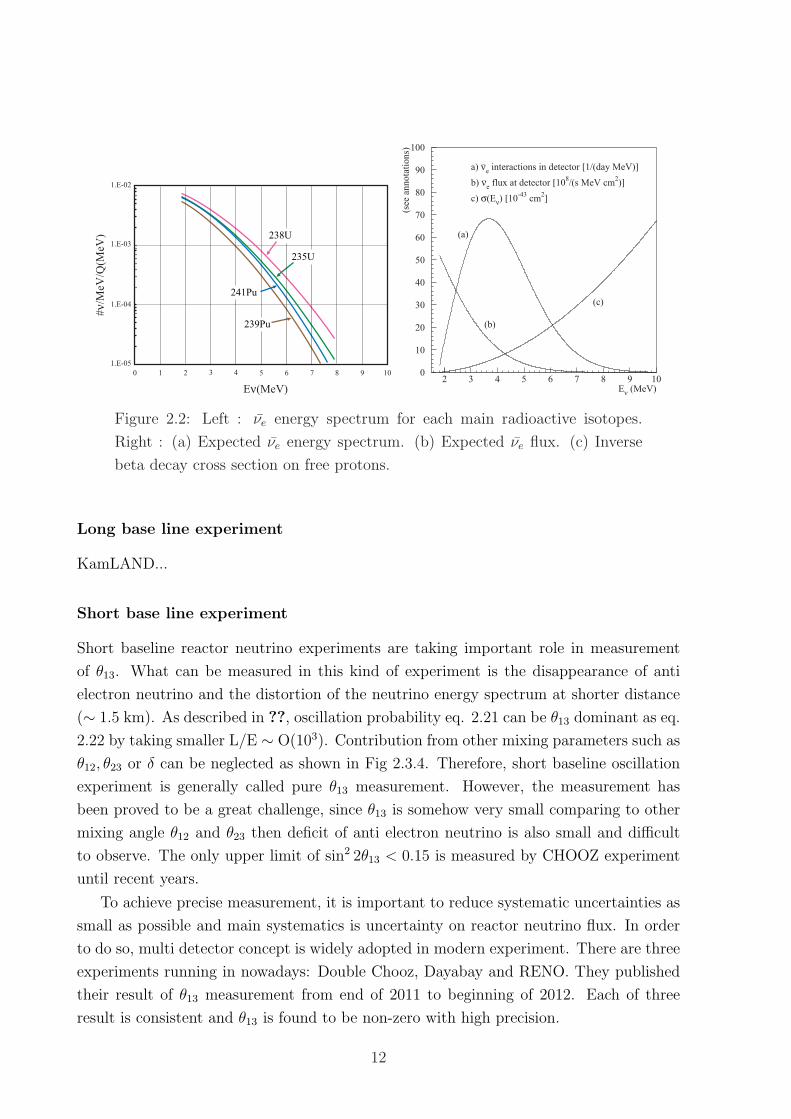
Figure 2.2: Left : νe energy spectrum for each main radioactive isotopes.
Right : (a) Expected νe energy spectrum. (b) Expected νe flux. (c) Inverse
beta decay cross section on free protons.
Long base line experiment
KamLAND...
Short base line experiment
Short baseline reactor neutrino experiments are taking important role in measurement
of θ13. What can be measured in this kind of experiment is the disappearance of anti
electron neutrino and the distortion of the neutrino energy spectrum at shorter distance
(∼ 1.5 km). As described in ??, oscillation probability eq. 2.21 can be θ13 dominant as eq.
2.22 by taking smaller L/E ∼ O(103). Contribution from other mixing parameters such as
θ12, θ23 or δ can be neglected as shown in Fig 2.3.4. Therefore, short baseline oscillation
experiment is generally called pure θ13 measurement. However, the measurement has
been proved to be a great challenge, since θ13 is somehow very small comparing to other
mixing angle θ12 and θ23 then deficit of anti electron neutrino is also small and difficult
to observe. The only upper limit of sin2 2θ13 < 0.15 is measured by CHOOZ experiment
until recent years.
To achieve precise measurement, it is important to reduce systematic uncertainties as
small as possible and main systematics is uncertainty on reactor neutrino flux. In order
to do so, multi detector concept is widely adopted in modern experiment. There are three
experiments running in nowadays: Double Chooz, Dayabay and RENO. They published
their result of θ13 measurement from end of 2011 to beginning of 2012. Each of three
result is consistent and θ13 is found to be non-zero with high precision.
12

L [km]-110 1 10 210
) eν → eν
P(
0
0.2
0.4
0.6
0.8
1
12θ + 13θ13θ12θ
= 0.113θ22, sin2 eV-310× = 2.5312m∆
= 0.8612θ22, sin2 eV-510× = 8.0212m∆
Reactor neutrino energy = 3 MeV
Nea
r de
tect
or
Far
det
ecto
r
Figure 2.3: Survival provability of 3 MeV anti electron neutrino as a function
of flight length. θ13 contribution is dominant up to few kilo meters. Detector
position of near and far are example of the Double Chooz.
Neutrino energy [MeV]2 4 6 8 10
) eν → eν
P(
0.8
0.85
0.9
0.95
1
12θ + 13θ13θ12θ
= 0.113θ22, sin2 eV-310× = 2.5312m∆
= 0.8612θ22, sin2 eV-510× = 8.0212m∆
Flight length = 1.05 km
Figure 2.4: Survival probability of anti electron neutrino as a function of neu-
trino energy at 1050 m from generation point. Distortion of neutrino energy
spectrum can be observed by oscillation effect.
Double Chooz
Double Chooz is subsequent experiment to CHOOZ experiment using two 4.2 GWth Chooz
reactor power plant. Using 102 days running data from single detector located at 1050 m
13

from reactor, first indication of reactor anti-neutrino disappearance is reported in Novem-
ber 2011 [15]. Rate and shape analysis are performed and sin2 2θ13 is found to be
sin2 2θ13 = 0.086± 0.041 (stat.)± 0.030 (syst.)
0.015 < sin2 2θ13 < 0.16 (90%C.L.)
The detail of the experiment is presented in Sec. 3.
DayaBay
The DayaBay nuclear power plant is located on the southern coast of China, 55 km to the
north-east of Hong Long. Anti electron neutrino generated from six reactors of 2.9 GWth
are detected by six detectors deployed in two near (flux-weighted baseline of 470 m and
576 m) and one far (1648 m) underground experimental halls. Each six identical detector
have 20 tons target volume filled with Gd doped liquid scintillator. Three of them are
placed at near experimental hall and others are at far hall.
Data taking with six detectors at both near and far site was started at Dec. 2011. The
first near-far cancellation analysis was performed and published in Mar. 2012[?]. Data
set and analysis was updated in May 2012 and the value of sin2 2θ13 is found to be
sin2 2θ13 = 0.089± 0.010 (stat.)± 0.005 (syst.)
(Ratiofar/near = 0.944± 0.007 (stat.)± 0.003 (syst.))
RENO
The RENO experiment observes anti electron neutrino from six 2.8 GWth reactors at the
Yonggwang nuclear power plant in Korea. Two identical detectors are located at near
(294 m) and far (1383 m) from the center of the reactors. Each detector has 16.5 tons
target volume of Gd loaded liquid scintillator. The data taking with both detectors is
started on August 2011. The first physics results based on 228 days of data was released
on April 2012 [?]. The result is obtained as,
sin2 2θ13 = 0.113± 0.013 (stat.)± 0.019 (syst.)
(2.36)
14
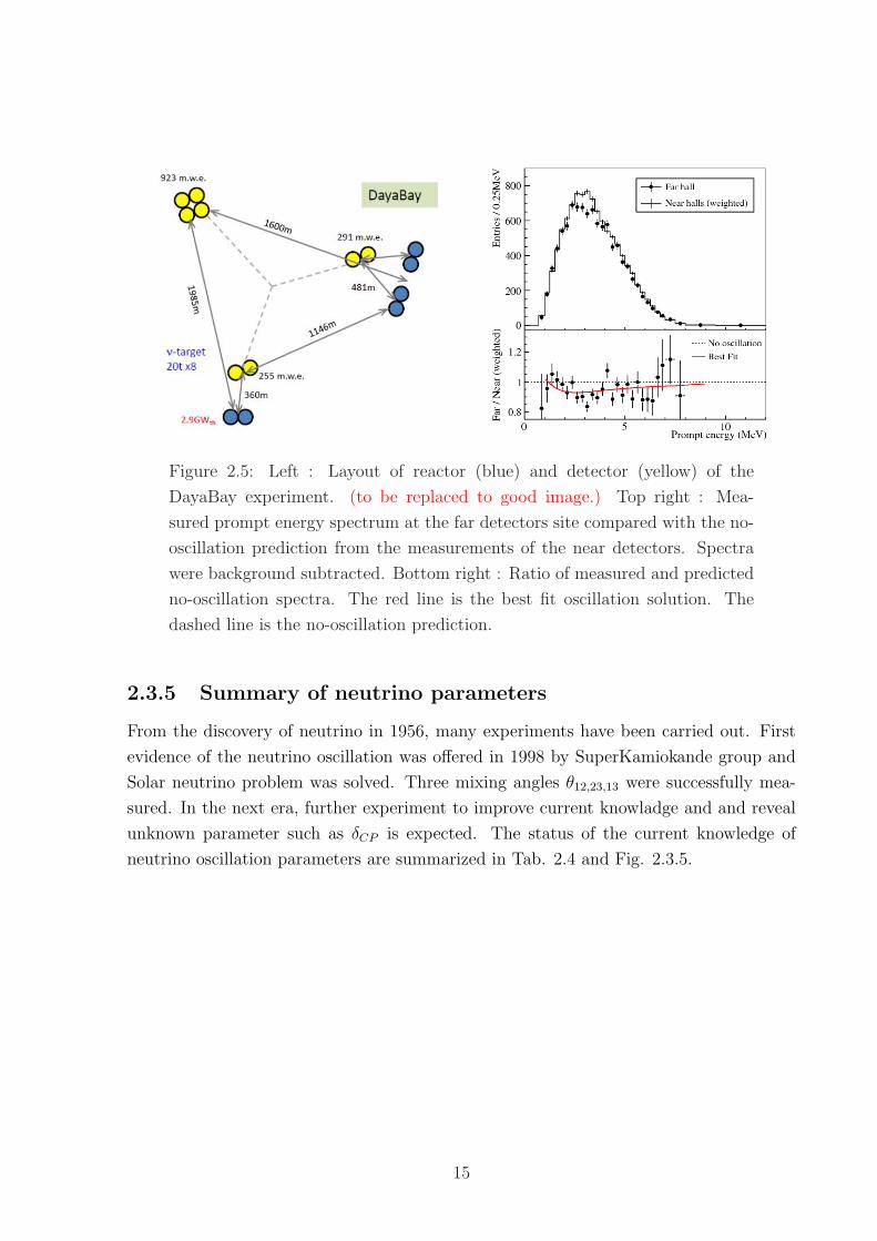
Figure 2.5: Left : Layout of reactor (blue) and detector (yellow) of the
DayaBay experiment. (to be replaced to good image.) Top right : Mea-
sured prompt energy spectrum at the far detectors site compared with the no-
oscillation prediction from the measurements of the near detectors. Spectra
were background subtracted. Bottom right : Ratio of measured and predicted
no-oscillation spectra. The red line is the best fit oscillation solution. The
dashed line is the no-oscillation prediction.
2.3.5 Summary of neutrino parameters
From the discovery of neutrino in 1956, many experiments have been carried out. First
evidence of the neutrino oscillation was offered in 1998 by SuperKamiokande group and
Solar neutrino problem was solved. Three mixing angles θ12,23,13 were successfully mea-
sured. In the next era, further experiment to improve current knowladge and and reveal
unknown parameter such as δCP is expected. The status of the current knowledge of
neutrino oscillation parameters are summarized in Tab. 2.4 and Fig. 2.3.5.
15

Figure 2.6: Left : Layout of reactor (blue) and detector (yellow) of the RENO
experiment. (to be replaced to good image.) Top right : Measured prompt
energy spectrum at the far detector compared with the no-oscillation prediction
from the measurements of the near detectors. The backgrounds shown in the
inserted figure are subtracted. Bottom right : Ratio of measured and predicted
no-oscillation spectra. The dashed line is the no-oscillation prediction.
Parameter best-fit (±1σ) 3σ
∆m221 [10−5eV2] 7.58+0.22
−0.26 6.99 - 8.18
∆m231 [10−3eV2] 2.35+0.12
−0.09 2.06 - 2.67
sin2 θ12 0.306 (0.312)+0.018−0.015 0.259 (0.265) - 0.359 (0.364)
sin2 θ23 0.42+0.08−0.03 0.34 - 0.64
sin2 θ13 0.251±0.0034 0.015 - 0.036
δCP to be measured to be measured
Table 2.4: The best-fit values and 3σ allowed ranges of the neutrino oscillation parameters,
derived from a global fit of the current neutrino oscillation data, including the Daya Bay
and RENO [?]. The values (in brackets) and no-brackets of sin2 θ12 are obtained using
(“new” [?]) and “old” [?] reactor νe fluxes in the analysis.
16

Cl 95%
Ga 95%
νµ↔ν
τ
νe↔ν
X
100
10–3
∆m
2 [
eV
2]
10–12
10–9
10–6
10210010–210–4
tan2θ
CHOOZ
Bugey
CHORUSNOMAD
CHORUS
KA
RM
EN
2
νe↔ν
τ
NOMAD
νe↔ν
µ
CDHSW
NOMAD
KamLAND
95%
SNO
95%Super-K
95%
all solar 95%
http://hitoshi.berkeley.edu/neutrino
SuperK 90/99%
All limits are at 90%CL
unless otherwise noted
LSND 90/99%
MiniBooNE
K2KMINOS
Figure 2.7: The regions of squared-mass splitting and mixing angle favored
or excluded by various experiments based on two-flavor neutrino oscillation
analysis[?]. The results from recent three reactor experiment (Double Chooz,
Daya Bay, RENO) are not included.
17

18

Chapter 3
The Double Chooz experiment
Double Chooz is one of the reactor neutrino experiments which aims to measure the
neutrino mixing angle θ13 with two identical detector concept. The experiment utilizes
the Chooz reactor power plant located at the boundary of France and Belgium. The
power plant has two pressurized water reactors which have a thermal power of 4.27 GW
for each. Figure 3.1 shows a bird’s-eye view of the CHOOZ power plant.
Construction of the far detector finished in 2010. After the detector commissioning,
physics data taking was started in 2011 spring. The expected sensitivity is 0.06 with 1.5
year running of only far detector and 0.03 with five years running of near and far detector
for the sin22θ13.
In this chapter, the experimental concept and detector design of the Double Chooz
experiment are described.
3.1 Neutrino detection principle
Reactor anti-neutrino is detected through inverse beta decay interaction with protons in
the detector,
νe + p→ e+ + n. (3.1)
The detection method called delayed coincidence technique is used from the first detection
of neutrino in 1953 by Reines and Cowan[3]. The inverse beta decay produce a positron
and a neutron. The positron annihilates with an electron immediately after energy de-
posit and produce two γ-rays (prompt signal). On the other hand, neutron is thermalized
through repeating elastic scattering with protons and captured by Gadolinium (Gd) nu-
cleon doped in liquid scintillator. After an average of ∼30 µs from the prompt signal,
The captured neutron then produces 8MeV γ-rays in total (delayed signal). The 8 MeV
signal is well-higher than the natural radioactive γ-rays which have maximum energy
of 2.6 MeV. Therefore, the background from natural radioactivities can be dramatically
19

Figure 3.1: Bird’s-eye view of the CHOOZ reactor power plant.
reduced. Neutrino signals are identified by those two signals and its time correlation.
The illustration of the detection scheme is shown in Figure 3.2. The threshold of in-
verse beta decay is calculated by assuming negligible neutrino mass and proton at rest.
Consequently:
Ethresholdβ =
(me+ +Mn)2 −M2p
2Mp
' 1.8 MeV, (3.2)
where me+ , Mp and Mp are the positron, neutron and proton masses, respectively.
The positron takes most of neutrino energy because the mass is so small comparing
to a proton. Hence, the neutron recoil can be neglected and neutrino energy can be
approximated from prompt signal as:
Eνe = Eprompt + Ethresholdβ − 2me = Eprompt + 1.8− 1.022 (MeV). (3.3)
3.2 Detector
The structure of the Double Chooz detector [?] is designed to accomplish better efficiency
for neutrinos and lower background comparing with the previous CHOOZ experiment[?].
Those improvements contribute to suppress systematic uncertainties in the experiment.
Figure 3.3 shows a schematic view of the Double Chooz detector.
20
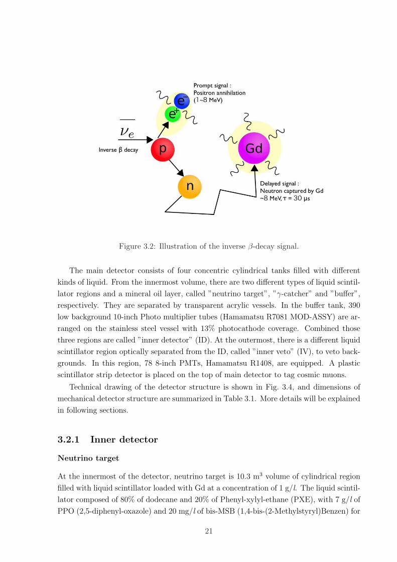
Figure 3.2: Illustration of the inverse β-decay signal.
The main detector consists of four concentric cylindrical tanks filled with different
kinds of liquid. From the innermost volume, there are two different types of liquid scintil-
lator regions and a mineral oil layer, called ”neutrino target”, ”γ-catcher” and ”buffer”,
respectively. They are separated by transparent acrylic vessels. In the buffer tank, 390
low background 10-inch Photo multiplier tubes (Hamamatsu R7081 MOD-ASSY) are ar-
ranged on the stainless steel vessel with 13% photocathode coverage. Combined those
three regions are called ”inner detector” (ID). At the outermost, there is a different liquid
scintillator region optically separated from the ID, called ”inner veto” (IV), to veto back-
grounds. In this region, 78 8-inch PMTs, Hamamatsu R1408, are equipped. A plastic
scintillator strip detector is placed on the top of main detector to tag cosmic muons.
Technical drawing of the detector structure is shown in Fig. 3.4, and dimensions of
mechanical detector structure are summarized in Table 3.1. More details will be explained
in following sections.
3.2.1 Inner detector
Neutrino target
At the innermost of the detector, neutrino target is 10.3 m3 volume of cylindrical region
filled with liquid scintillator loaded with Gd at a concentration of 1 g/l. The liquid scintil-
lator composed of 80% of dodecane and 20% of Phenyl-xylyl-ethane (PXE), with 7 g/l of
PPO (2,5-diphenyl-oxazole) and 20 mg/l of bis-MSB (1,4-bis-(2-Methylstyryl)Benzen) for
21

Figure 3.3: Schematic view of the Double Chooz detector.
Detector Inner Inner Vessel Filled Liquid Weight
volume diameter [mm] height [mm] thickness [mm] with volume [m3] [tons]
Target 2,300 2,458 8 Gd-LS 10.3 0.35
γ-catcher 3,392 3,574 12 LS 22.6 1.1-1.4
Buffer 5,516 5,674 3 Oil 114.2 7.7
Inner veto 6,590 6,640 10 LS 90 20
Shielding 6,610 6,660 170 Steel - 300
Pit 6,950 7,000 - - - -
Table 3.1: Dimensions of the mechanical detector structure.
the wavelength shifters. PXE and dodecane are ionized and excited by energy depositions.
Then the energy is transferred non-radiatively to a PPO molecule and finally to bis-MSB
22

Figure 3.4: Technical drawing of the Double Chooz detector.
that shifts the emission light frequency. The re-emission wavelength is peaked around 430
nm, which matches a peak of quantum efficiency of the PMT used in this experiment. This
type of Gd-loaded scintillator is developed and used in various reactor neutrino experi-
ment. However, some experiments like CHOOZ and Palo Verde [?] observed degradation
of their liquid scintillator due to material incompatibility with detector. Hence, long-term
stability of scintillator at least 5 years is an important requirement for our the experiment.
Liquid scintillator for the Double Chooz experiment is developed by Max Planck Institute
for nuclear physics (MPI-K) group. Material compatibilities, optical properties, safeness
and its long-term stability were tested. Figure 3.5 shows transmission as a function of the
wavelength measured in MPI-K.
23

300 400 500 600 700 8000
10
20
30
40
50
60
70
80
90
100
! (nm)
Tra
nsm
issio
n (
%)
0 day
33 days
60 days
130 days
174 days
214 days
242 days
350 days
398 days
20 % PXE 80 % Dodecane& Fluors
Gd!carbox sample 3
Closed cell control test @ 20 oC
300 400 500 600 700 8000
10
20
30
40
50
60
70
80
90
100
! (nm)
Tra
nsm
issio
n (
%)
0 day
33 days
60 days
130 days
174 days
214 days
242 days
350 days
398 days
20 % PXE 80 % Dodecane& Fluors
Gd!carbox sample 3
Closed cell control test @ 40 oC
Tra
nsm
issio
n (
%)
Figure 3.5: Transmission as a function of the wavelength for various time elapsed sample.
Left: Accelerated aging test with 40C. Right: stored at room temperature.
γ-catcher
The γ-catcher is a 55 cm-thick volume surrounding neutrino target filled with 22.3 m3 of
non-Gd scintillator. Neutrino target and γ-catcher vessels are built from acrylic plastic
material, transparent to UV and visible photons with wavelengths above 400 nm. The
volume intends to detect the γ-ray escaped from target region to ensure the energy recon-
struction. The scintillator composition is 30% of dodecane, 66% of ondina 909 and 4% of
PXE with 2 g/l of PPO and 20 mg/l of bis-MSB. In order to keep detector uniformity,
the LS was produced as same light yield per deposit energy.
Non-scintillating buffer
A 105 cm-thick region encloses the γ-catcher and Neutrino target. Buffer vessel is made
from stainless steel and 390 10-inch PMTs are arranged on inside of vessel to detect
scintillation light. 114.2 m3 of non-scintillating mineral oil is filled in this region in order
to reduce natural radioactivity background which mainly come from PMT glass.
3.2.2 Inner veto
At the outermost of the detector, there is a region of 50 cm thickness called Inner Veto,
which is optically separated from the buffer. Inner veto filled with a liquid scintillator
made of 50% decane to tridecane (decane, undecane, dodecane, tridecane) and 50% LAB
(lineares alkylbenzene) with 2g/l of PPO and 20 mg/l of bis-MSB. Composition of liquids
used in Double Chooz detector are summarized in Table 3.2. The main purpose of the
Inner veto is to detect cosmic muon passing through or near the Inner detector moreover,
detect muon-induced background like fast-neutron coming from outside of the detector
24

with very high efficiency. In order to maximize the light correction efficiency, VM2000
high reflective foils and paint have respectively been used on the outer buffer wall and on
the inner veto tank wall. Those coatings increase the light collection by more than factor
2. Inner veto PMTs are 8-inch Hamamatsu R1048 [?] encapsulated in a stainless steel
cone, these PMTs were used in IMB [?] and SuperKamiokande experiments. A combined
quantum and collection efficiency is 20% in the relevant wavelength. In order to maximize
an efficiency and minimize a cost, arrangement of IV PMTs was studied by Monte Carlo
simulation [?]. Due to the rather small space between these two walls, total 78 PMTs
are oriented parallel to the surface with 0.6% photo coverage and > 99.9% efficiency.
Arrangements of 78 PMTs are shown in Fig. 3.6.
Outside of Inner veto vessel, a low activity steel shielding 170 mm-thick is protecting
the detector from the natural radioactivity of the rocks around the pit.
Figure 3.6: Transparent view of detector showing arrangement of Inner veto PMTs.
3.2.3 Outer veto
Additional muon tagging and tracking detector so called Outer Veto (OV) is installed on
the top of the main cylindrical detector. OV has upper and lower planes. Lower plane
is paved with 36 modules and 8 modules for upper plane. Each module consists of two
25

Components Solvent Primary solution Secondary solution Gd(dpm)3Target Dodecane (80 %) PPO (7 g/l) bis-MSB (20mg/l) 4.5 g/l
PXE (20 %)
γ-catcher Dodecane (30 %) PPO (2 g/l) bis-MSB (20mg/l) -PXE (4 %)
Mineral oil (66 %)
Buffer Mineral oil (∼50%) - - -Tetradecane (∼50%)
Inner veto LAB (38 %) PPO (2 g/l) bis-MSB (20mg/l) -Tetradecane (62%)
Table 3.2: Compositions of Double Chooz liquids.
layers of 32 plastic scintillator strips (5 × 2 × 320 cm) with wavelength-shifting fibers.
Scintillation lights generated in a scintillator strip is collected through fibers and detected
by multi-anode PMTs. Figure 3.7 and 3.8 show schematic views of OV module and its
arrangement. OV detector can reconstruct vertices where muons interact by coincidences
of different layers and different X-Y dimensional modules with very high resolution (∼few cm). Furthermore, muon track can be reconstructed by coincidence of upper and
lower plane. Total dimension is 6.4 × 12.8 m2 for the lower plane and 3.2 × 6.4 m2 for
upper plane. In addition to IV detected muons, this extended detector provide efficiency
for near-miss muons which could not be detected by IV whereas cause fast neutrons from
interaction with surrounding rock. For the near detector, larger area of OV detector with
11.0 × 12.8 m2 will be implemented because of higher rate muons due to the shallow
depth at the near detector laboratory. In this thesis, only lower plane of OV detector was
in operation. The trigger rate of OV lower plane is ∼2.7 kHz.
3.2.4 Calibration system
The calibration system plays an important role in precise experiments. We must accu-
rately know neutrino signal efficiency and its energy since the θ13 is measured by observing
a few percent of deficit in neutrino rate and it energy distortion with respect to the pre-
diction. Several calibration systems are implemented in the Double Chooz detector to
achieve the precise measurement of θ13, as follows:
Light injection system
Inner Detector Light Injection system (IDLI) is embedded on the Inner-detector PMT
and used for PMT gain and timing calibration. The light from LEDs are transported into
26

6 March 2009 Double Chooz Meeting 2
3225 mm
3625 mm
Mirrored fiber ends
Scintillator strips
Fiber routing
Al skin for module
Fiber holder
M64
FE card
Figure 3.7: A schematic view of the layout of scintillator strip in a OV module.
X layer
Y layer
Figure 3.8: Arrangement of OV modules. Top : X layer modules which provides vertex
position of Y. Bottom : Y layer modules laying on X layer modules provides vertex
position of X.
the detector through an optical fiber arranged along edge of µ-metal (Fig. 3.9). We drive
three types of LEDs emitting different wavelength; λ =385, 425 and 475 nm. Light with
λ =385 nm will be absorbed by the scintillator and then re-emitted. Light with λ =425
27

and 475 nm can pass through the scintillator and reach directory to the PMTs. Intensity
of light is monitored by PIN photodiode and can be controlled from one photoelectron to
several hundred photoelectron level. At the end of fiber, there is a diffuser which spread
the light over the angle of about 22 degrees, or a quartz fibers providing a more narrow
light (about 7 degrees) called pencilh beam. Diffused light is used for PMT gain and
timing calibration and the stability check.
Figure 3.9: Picture of IDLI fiber.
Figure 3.10: Illustration of diffused light. Figure 3.11: Illustration of pencil light.
Radioactive source and deployment system
Response of liquid scintillator and detector are depending on various factors such as
energy, kind of particles (α, β, γ), or vertex of the interaction. Hence, several kind of
28

radioactive sources with deployment system are embedded in the Double Chooz detector.
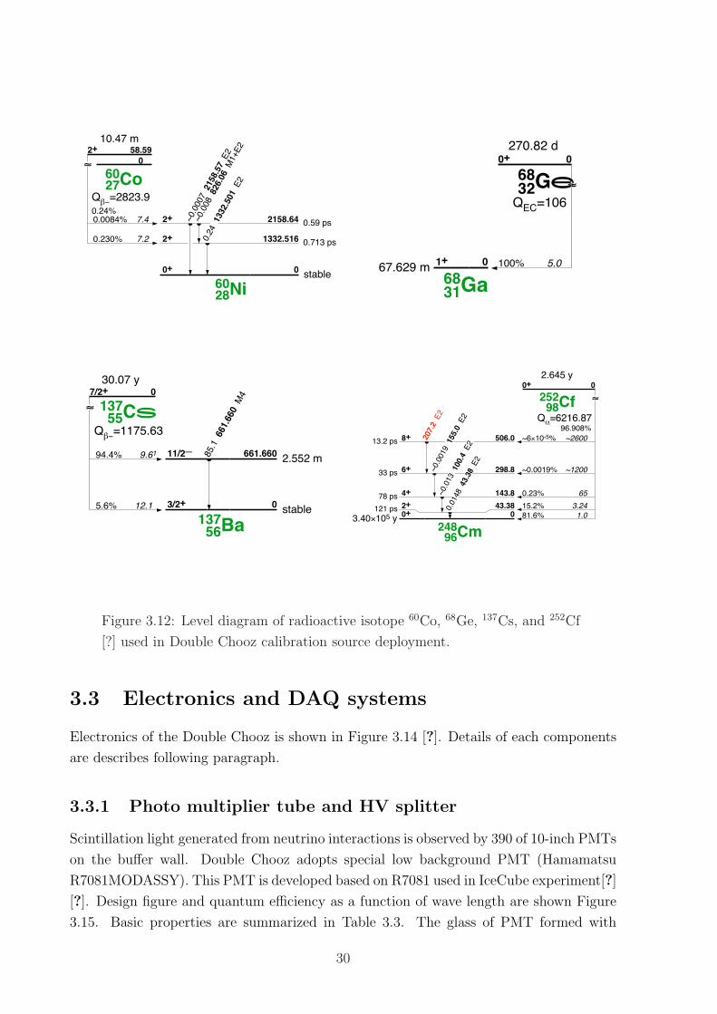
• 68Ge
68Ge decays by the electron capture to 68Ga, then which decays to stable 68Zn
by e+-decay. Finally, two annihilation gammas which has 1.022 MeV in total are
produced. This energy corresponds to the minimum prompt signal for IBD reaction,
thus allowing to calibrate the efficiency of the trigger threshold at different positions
to make sure all IBD positrons are accepted.
• 252Cf
252Cf emits several neutrons with average multiplicity of 3.76. It can be used to
study neutron efficiency and position dependence of that, in particular close to the
boundary between target and gamma catcher which is called spill-in-out effect. The
neutron energy spectrum of 252Cf is softer than the one of the AmBe source and has
an average of approximately 2.1 MeV.
• 137Cs
137Cs emits 0.662 MeV mono-energetic γ-ray that can be used to calibrate scintil-
lator energy scale with half-life of 30.07 years.
• 60Co
60Co emits 1.17 and 1.33 MeV γ-rays with half-life of 5.27 years.
Level diagram of each isotopes are shown in Fig 3.2.4.
Z-axis deployment system
The Z-axis deployment system allows the radioactive sources to be deployed in the target
along the central axis of the detector from the glove box. This system is used to calibrate
energy response in the target.
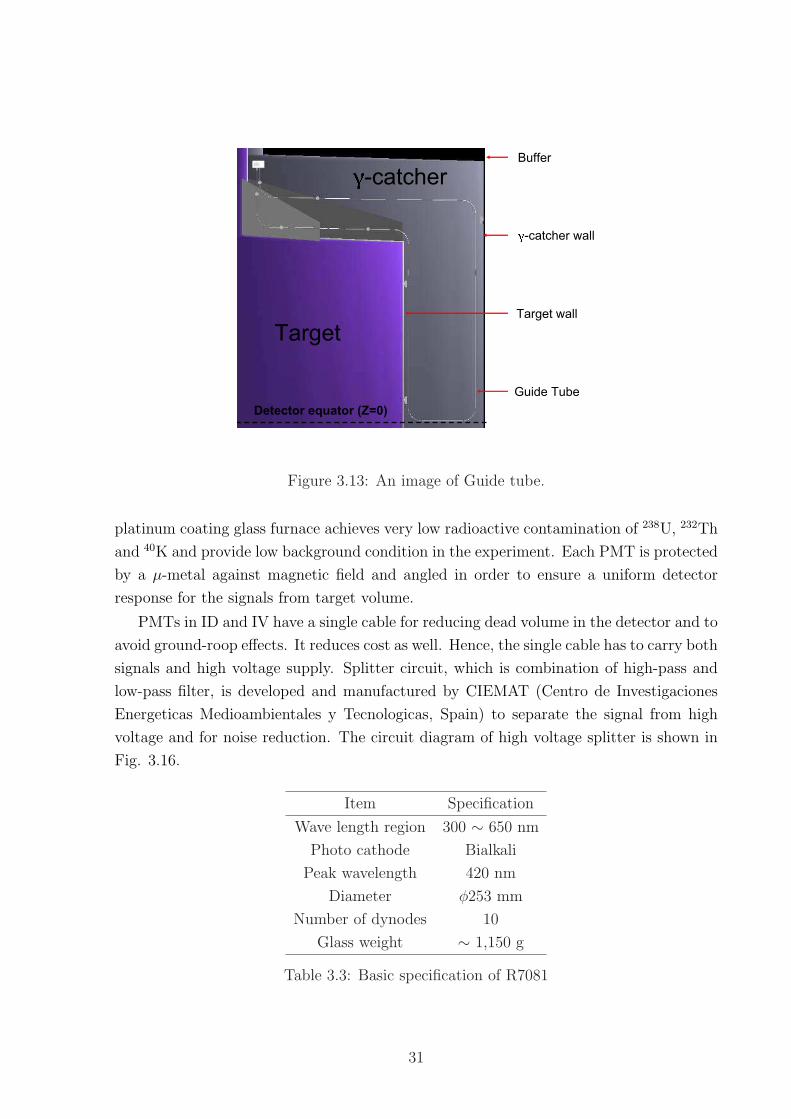
Guide tube system
Guide tube is a double teflon tube to deploy a radioactive sources into the Gamma-catcher
region. The tube is installed along with ν-target and γ-catcher acrylic vessels (Fig. 3.13).
At the boundary of the ν-target region, spill-in effect, which the IBD interaction occurs
in γ-catcher region but neutron got into the target region and produce 8MeV gammas,
should be take into account. This system is used for the study of energy response in the
γ-catcher and spill-in effect.
29
60 28Ni
00+
1332.5162+
2158.642+ ~0.0
007 2158.5
7 E
2
~0.0
08 826.0
6 M
1+E
2
0.2
4 1332.5
01 E
2
stable
0.713 ps
0.59 ps
60 27Co
0!
0.230% 7.2
0.0084% 7.4
2+ 58.59
10.47 m
Q"#=2823.90.24%
68 31Ga
01+ 67.629 m
68 32Ge !
100% 5.0
0+ 0
270.82 d
QEC
=106
137 56Ba
03/2+
661.66011/2Ð 85.1
661.6
60 M
4
stable
2.552 m
137 55Cs!
5.6% 12.1
94.4% 9.61
7/2+ 0
30.07 y
Q"#=1175.63
248 96Cm
00+43.382+
143.84+
298.86+
506.08+ 207.2
E
2
~0.0
019 155.0
E
2
~0.0
13 100.4
E
2
0.0
148 43.3
8 E
2
3.40!105 y 121 ps
78 ps
33 ps
13.2 ps
252 98Cf "
81.6% 1.0
15.2% 3.24
0.23% 65
~0.0019% ~1200
~6!10-5% ~2600
0+ 0
2.645 y
Q#=6216.87
96.908%
Figure 3.12: Level diagram of radioactive isotope 60Co, 68Ge, 137Cs, and 252Cf
[?] used in Double Chooz calibration source deployment.
3.3 Electronics and DAQ systems
Electronics of the Double Chooz is shown in Figure 3.14 [?]. Details of each components
are describes following paragraph.
3.3.1 Photo multiplier tube and HV splitter
Scintillation light generated from neutrino interactions is observed by 390 of 10-inch PMTs
on the buffer wall. Double Chooz adopts special low background PMT (Hamamatsu
R7081MODASSY). This PMT is developed based on R7081 used in IceCube experiment[?]
[?]. Design figure and quantum efficiency as a function of wave length are shown Figure
3.15. Basic properties are summarized in Table 3.3. The glass of PMT formed with
30
Target
-catcher
Detector equator (Z=0)
Target wall
-catcher wall
Buffer
Guide Tube
Figure 3.13: An image of Guide tube.
platinum coating glass furnace achieves very low radioactive contamination of 238U, 232Th
and 40K and provide low background condition in the experiment. Each PMT is protected
by a µ-metal against magnetic field and angled in order to ensure a uniform detector
response for the signals from target volume.
PMTs in ID and IV have a single cable for reducing dead volume in the detector and to
avoid ground-roop effects. It reduces cost as well. Hence, the single cable has to carry both
signals and high voltage supply. Splitter circuit, which is combination of high-pass and
low-pass filter, is developed and manufactured by CIEMAT (Centro de Investigaciones
Energeticas Medioambientales y Tecnologicas, Spain) to separate the signal from high
voltage and for noise reduction. The circuit diagram of high voltage splitter is shown in
Fig. 3.16.
Item Specification
Wave length region 300 ∼ 650 nm
Photo cathode Bialkali
Peak wavelength 420 nm
Diameter φ253 mm
Number of dynodes 10
Glass weight ∼ 1,150 g
Table 3.3: Basic specification of R7081
31

Energy deposit
ID-PMTHamamatsu
R7081MODASSY390 PMTs (10Ó)
IV-PMTHamamatsu R1408
78PMTs (8Ó)(from IMB)
HV-SplitterCIEMAT(custom)
HV-SupplyCAEN
SY1527LCA1535P
FEEgain~7
(custom)
VME Crate~16 FADC cards
DAQ software in Ada
Trigger & Clock SystemID: Energy
IV: Energy & pattern62.5MHz clock
MVME3100
22m ID26m IV
18m
ID 16:1IV !6:1
PMT Splitter FEE
HV Trigger
!-FADC500MHz
CAEN-V1721
"-FADC125MHz(custom)
Computers
Figure 3.14: Electronics of the Double Chooz.
Figure 3.15: Design of Hamamatsu R7081 MOD-ASSY and its quantum efficiency as a
function of wave length.
3.3.2 High voltage system
Double Chooz adopted an universal multichannel power supply system manufactured
by CAEN [?]. Figure 3.17 shows the picture of HV main frame SY1527LC and A1535P
module. This HV is used for 390 PMTs for the Inner detector and 78 PMTs for Inner veto.
Thus, total 468 channel of HV are needed. The SY1527 frame has 16 slots for module input
and A1535 has 24 channels for high voltage output. Main properties are summarized in
Table 3.4. In order to uniform the gain of PMTs, the HV system have to provide different
32

Figure 3.16: The circuit diagram of the splitter. Combination of high-pass and low-pass
filter separate signal and HV. Additionally, noise from HV system can be reduced.
voltages to PMTs individually. In Double Chooz, precise measurement of neutrino energy
is a essential to improve the sensitivity and realize the precise measurement of θ13. The
energy is reconstructed from the signal charge of PMTs, hence the high voltage which
directly affects PMT gain is taking an important role in the experiment.
The precision of the output voltage, long term stability of that and HV produced noise
level have been tested. CAEN high voltage system shows good performance to use for
Double Chooz experiment[?].
Figure 3.17: Picture of High Voltage crate and module.
33

Polarity Positive
Output Voltage 0∼3.5 kV
Max. Output Current 3 mA
Voltage Set/Monitor Resolution 0.5 V
Current Set/Monitor Resolution 500 nA
Hardware Voltage Max 0∼3.5 kV
Hardware Voltage Max accuracy ±2 % of Full Scale Range
Software Voltage Max 3.5 kV
Software Voltage Max accuracy 1 V
Ramp Up/Down 1 ∼ 500 V/sec, 1 V/sec step
Voltage Ripple <20 mV typical; 30 mV max
Voltage Monitor vs. Output Voltage Accuracy typical: ±0.3 % ±0.5 V
max:±0.3 % ±2V
Voltage Set vs. Voltage Monitor Accuracy typical: ±0.3 % ±0.5 V
max:±0.3 % ±2V
Current Monitor vs. Output Current Accuracy typical: ±2 % ±1 µA
max:±2 % ±5 µA
Current Set vs. Current Monitor Accuracy typical: ±3 % ±1 µA
max:±2 % ±5 µA
Maximum output power 8W(per channel, soft ware limit)
Power consumption 310 W @ full power
Table 3.4: Properties of CAEN A1535P module
34

3.3.3 Front End Electronics and Flash ADC
Signals from PMTs are separated from high voltage by splitter then sent to front end
electronics (FEE). The FEEs amplify the signals from the Inner detector by a factor of
7.8 to match the dynamic range of following Waveform digitizers(Flash ADC). On the
other hand, signals from the Inner veto events are amplified by a factor of 0.55. The
gain factor is smaller than that of ID since muon events emit large amount of scintillation
lights in IV. In addition, FEE reduces noise in the incoming signal and keep the baseline
voltage stable.
The FEE also sums up analog signals for 8 channels and send stretcher signal to the
trigger system. The stretcher signal has a pulse height proportional to the charge sum of
analog signals.
Signals from FEE are send to CAEN VX1721 flash ADCs shown in Figure 3.18, those
were developed by CAEN SpA with APC (Astro Particule et Cosmologie, Paris)[?].
Each module houses eight channels for input with dynamic range of 1000 mV (8 bit
resolution). The 500 MHz sampling rate provides 2 ns timing resolution. Each channel has
2 MB memory split into pages. The number of pages is adjustable. In case of 1024 pages,
each one can store 2048 samples for a total of 4 µs of digitized data. In the experiment,
time window is set to 256 ns for extra data reduction.
Figure 3.18: Picture of CAEN VX1721 flash ADC board.
3.3.4 Trigger system
ID trigger system consists of three trigger boards (TB) and one trigger master board
(TMB)[?]. Two identical trigger board named TB-A and TB-B are implemented for
inner detector (ID) and one trigger board (TB-IV) is implemented for the inner veto (IV).
Figure 3.19 shows a schematic overview of the system. TB-A and TB-B has 13 inputs,
with each input being an analog sum of 16 PMTs formed by the Front End Electronics
(only one input has 3 PMTs signal sum). TB-IV has 18 inputs with 3 ∼ 6 PMTs signal
sum.
In each input, trigger condition is checked at the end of each 32 ns clock cycle and
to release a trigger signal in case of a fulfilled condition. Discrimination is performed by
35
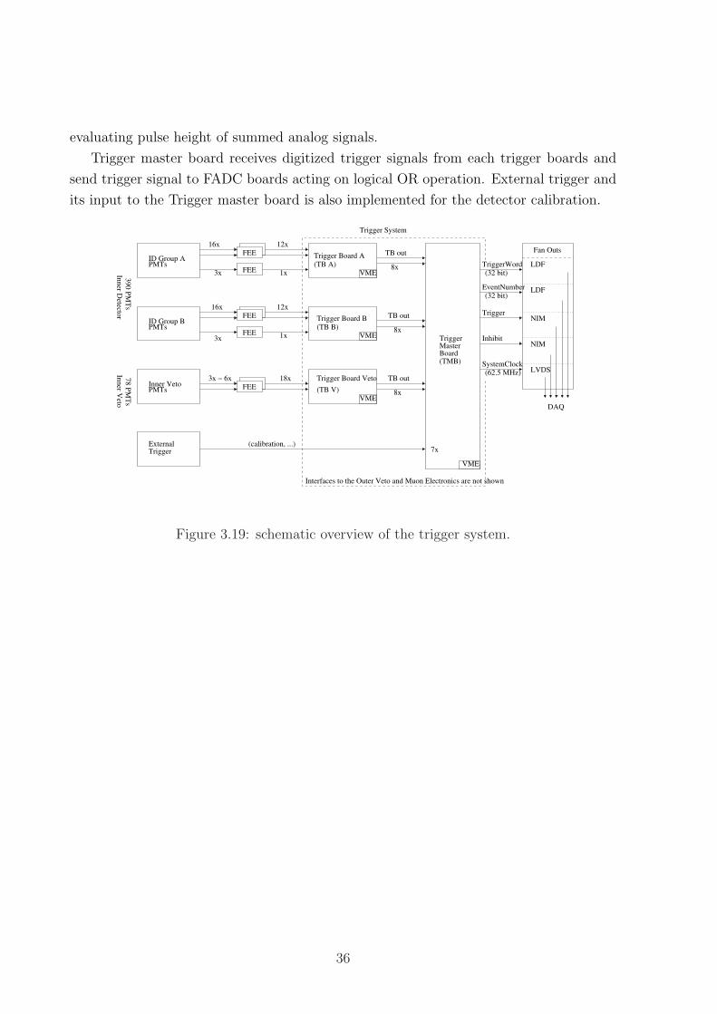
evaluating pulse height of summed analog signals.
Trigger master board receives digitized trigger signals from each trigger boards and
send trigger signal to FADC boards acting on logical OR operation. External trigger and
its input to the Trigger master board is also implemented for the detector calibration.
ID Group APMTs
ID Group B
Inner Veto
PMTs
PMTs
ExternalTrigger
FEE
FEE
FEE
FEE
FEE
VME
VME
VME
Trigger Board A
Trigger Board B
Trigger Board Veto
TriggerMasterBoard
Fan Outs
EventNumber
TriggerWord
Trigger
Inhibit
SystemClock
LDF
LDF
NIM
NIM
LVDS
VME
(62.5 MHz)
(32 bit)
(32 bit)
(TMB)
16x
18x
TB out
TB out
8x
8x
TB out
8x
7x(calibration, ...)
16x
3x
12x
1x
12x
3x 1x
3x − 6x
Trigger System
Interfaces to the Outer Veto and Muon Electronics are not shown
(TB A)
(TB B)
(TB V)
Inn
er Veto
78 P
MT
s390
PM
Ts
Inn
er Detecto
r
DAQ
Figure 3.19: schematic overview of the trigger system.
36

Chapter 4
Event Reconstruction and Detector
Calibration
In this chapter, event reconstruction for the Double Chooz is presented. In Double Chooz,
390 PMTs detects scintilaltion light generated from energy deposit inside the detector.
Signals from PMT are amplified and digitized by FADCs. Firstry, we sums up digitysed
pulses from each PMTs by impremented pulse reconstruction algorithm. Secondary, in-
tegrated charge is converted to number of photo-electrons by deviding total charge by
calibrated PMT gains. Reconstructed P. E. is finaly transrated to reconstructed energy
considering event vertex, non-linearity of FADC, and stability. Overview of event re-
construction flow is shown in Fig. 4.1. The detail of each reconstructions and detector
calibration method is presented in this chapter. Additionally, muon track reconstruction
method is also presanted.
Energy deposit
PMTs
MeV P. E. Charge
ChargeP. E.
FADCElectronics
Pulse reconstruction
PMT gain
MeV
Energy reconstruction - non linearity - vertex - stability
TrueReconstructed
Figure 4.1: Schematic view of event reconstruction flow.
37

4.1 Pulse reconstruction
Pulse resonstruction and charge calculation tool for DC is impremented and called DCRe-
coPulse[?]. The main purpous of this tool is to provide us total charge and timing infor-
mation of the pulses that we observed. The DCRecoPulse performs following functions.
Baseline calculation
This is the first step to get correct charge and timing information. Two method for baseline
calculation are impremented. One is performed by making use of external triggere event
produced every second(1Hz clock cicle). The mean of all ADC values is computed and
then the sample with the largest deviation from the mean is removed, thus pushing the
mean of the remaining ADC values to the attest region of the readout. This process is
iterated until largest and lowest ADC values have same deviation, within a tolerance of 1
ADC count (or DUI). This method is called External baseline method. Another method
called Floating baseline method is also impremented. In this method, baseline calculation
is performed every self-triggered physics events by taking baseline samples in the biggining
of readout window. Only 10 bins of FADC (20ns) are used for calculation. Both of those
methods have cirtain advantage and also disadvantage.
The External baseline method allows more precise estimation in a typical, however
suffers from baseline shift occures after huge muon-like signals. On the other hand, the
Floating baseline method is more stable against baseline fluctuation but has some draw-
back in accuracy of calculation due to its smallness of integrated window. For example, if
some pre-pulse or dark noise arise in this region, baseline could not be calculated correctly.
Moreover, large pulse get across the FADC time window also hide baseline in integrated
part.
We adopt hibrid method extracting good point of both methods. Namely, the numbers
of both method, mean and RMS value of the baseline, are calculated, then the values of
Floating method is adopted by default. However, if RMS of Floating method is more
than 0.5 DUQ2 larger than that of Extrnal method, former one is considered unreliable,
and the number of External method is adopted.
Pulse charge calculation
After the baseline subtraction, total charge is calculated by integrating ADC counts inside
the fixed-size time window. The time window slides to analyse another part of waveform.
The window position that has the maximum integral is assumed to contain the pulse.
In principle, the algorithm then reiterates and searches for possible other pulses in the
38

Mean 244.5RMS 0.1093
Amp (DUI)243 243.5 244 244.5 245 245.5 246
Ent
ries
0
100
200
300
400
500
600
700
Mean 244.5RMS 0.1093
Mean 125RMS 0.9086
Num. samples120 122 124 126 128 130
Ent
ries
0
100
200
300
400
Mean 125RMS 0.9086
Figure 4.2: Pedestal mean estimation of a sample of 1000 simulated 1PE pulses
with a pedestal level of 244.5 DUI. Left: pedestal mean estimation according to
the External baseline method (solid line), and to the Floating baseline method
assuming a 40 ns window (dashed line). Right: number of time samples used
for the pedestal estimation when using the External baseline method.
waveform, until the the maximum integral in a window falls below the threshold.
Qmin = nσ · σped ·√WS; (4.1)
where nσ is the constant number defined by user, σped is RMS of baseline and WS is the
size of time window set to 112ns by default.
Pulse timing analysis
The DCRecoPulse compute the following timing caracteristics for each found pulse.
• Start time
Time corresponds to 30% of the maximum amplitude before it is reached.
• End time
Time corresponds to 20% of the maximum amplitude, after it was reached.
• Maximum amplitude time
Time corresponding to maximum of the pulse
• Rise time
Time defined as the difference between the maximum amplitude and start times.
39

• Fall time
The fall time is defined as the difference between the end and maximum amplitude
times
4.2 Vertex reconstruction
Vertex reconstruction for the Double Chooz detector is performed by maximum likelihood
method using charge and timing information[?, ?]. Events will be reconstructed is assumed
to be a point-like source produces isotropic light of strength per solid angle Φ (photon/sr).
The expected light at any given PMT can be calculated with simple imaging detector
model, where light propagation is only affected by pure attenuation.
µi = εi × Φ× Ωi × exp(−ri/λ), (4.2)
where εi is quantum efficiency, Ωi is the solid angle subtended by the PMT, ri is the
distance from the source, and λ is the characteristic attenuation length. Assuming the
angular responce function of the ith PMT to be f(cos ηi), where ηi is the angle of incidence
of the light with respect to the ith PMT normal. The solid angle subtended by the ith
PMT with radious R can be written with a approximation (R ¿ ri) as
Ωi = πR2 × f(cos ηi)
r2i
. (4.3)
The optical model is used to predict the amount of light the PMTs see. It is fully
characterized λ and f cos(η). These allow then to calculate the total amount of light
created in an event, which is basically proportional to its total energy. They are essentially
the probability of µi measuring a certain charge where is expected. The timing likelihood
is also obtained simplified detector model as
tpredi = t0 +
ri
cn(4.4)
where cn is the effective speed of light in the scintillator. The event likelihood is defined
as
L(X) =∏qi=0
fq(0;µi)∏qi>0
fq(qi;µi)ft(ti; tpredi , µi) (4.5)
where the first product goes over the PMTs that have not been hit, while the second
product goes over the remaining PMTs that have been hit (i.e., have a non-zero recorded
charge qi at the registered time ti ). fq(qi;µi)is the probability to measure a charge qi
given an expected charge µi, and ft(ti; tpredi , µi) is the probability to measure a time ti
given a prompt arrival time tpredi and predicted charge µi. These are obtained from MC
40

simulations. The task of the event reconstruction is to find the best possible set of event
parameters Xmin which maximizes the event likelihood L(X).
The ideally simplified concept and method of vertex reconstruction is presanted so far,
however, the responce of real detector is complicated in fact. For the cahrge likelihood
function, quantum efficiency of PMTs are not uniform even on their own photocathode
and must be depending on incident angle of photons. Collection efficiency (efficiency of
first diode for generated photoelectron) is also have PMT dependence. Moreover, PMT,
electronics, readout systems have finite energy resolutions of cource. For the timing
function, the situation is much more complicated. The pulses from individual PMTs may
take different time to propagate through the different lengths cables and internal delays
in the electronic circuits. So that, it is required so called “T0 calibration”, which would
equalize the time offsets of individual PMTs and correct the raw pulse time reported by
the RecoPulse. In addition, the time profile of the light emission by a scintillator is not a
delta-function, and has a sharp rise and then decays exponentially with one or more time
constants. The light propagation itself suffers from exponential attenuation, reflections or
scattering at the boundaries between different media inside the detector. To make things
worse, the speed of light is wave-length dependent and may generally differ in different
media. Those parameter in Monte Carlo should be tuned from real calibration data. The
UV laser calibration system with multiple intensities is under preparation. The system
can be used for detector calibration and MC tuning in future.
Figure 4.3, 4.2 shows performance of vertex reconstruction on calibration source data.
As it mentioned at bigging of this section, this algorithm construct with point like source
assumption hence can reconstruct only point like energy deposit events. Events which
widely depositting energy, like muon crossing the detector could not be reconstructed
correctry. Other reconstruction algorithms for muon track reconstruction are also impre-
mented in DC and described in next section.
4.3 Energy reconstruction
4.3.1 PMT gain calibration
PMT gain calibration is a first step for the energy reconstruction and important for all
analysis. This gives a number of photo-electron(P.E.) reconstructed from charge observed
by each PMTs. Due to the uncertainty on the baseline of FADC, observed gain is differs
according to amount of signals. This behavior is called “gain non-linearity”. In order to
resolve this problem, two method for extract the gain for both low-charge and high-charge
signals are performed. After that, two method are combined to obtain so-called linearized
P.E.. The PMT gain calibration is performed using diffused light from lightinjection
41

[mm] true - XrecX-1000 -500 0 500 1000
Eve
nts
0
2000
4000
6000
8000 MC
DATA
Figure 4.3: The vertex destribution for Co-60 events. Source was positioned at the
detector center. Data histogram is background-subtracted.
Z position[mm] -1500 -1000 -500 0 500 1000 1500
Bia
s [m
m]
-50
0
50
100
DATA
MC
Z position [mm] -1500 -1000 -500 0 500 1000 1500
Res
olut
ion
[mm
]
60
80
100
120
140
160DATA
MC
Figure 4.4: Reconstruction bias and resolution are defined as mean and sigma
oftained by gaussian fitting of Figure 4.3. Left: Reconstruction bias as a
function of Z position. Right: Resolution of vertex reconstruction as a function
of Z positoin.
system (IDLI) with low and high intensity.
Single P.E. calibration
The diffused light of IDLI system is useful for illuminate all PMTs. Wavelength of emitted
light is set to 425nm optimesed for allowing PMTs to give a maximum quantum efficiency.
The Single P.E. calibration is performed by fitting the obtained single P.E. peaks(Fig. 4.5).
Hence, in order to obtain pure single P.E. peak, very low intencity light which produce
much lower signal than single P.E. level in avalage is used. The charge distribution
is considered to obey a Poisson and Gaussian distribution. Poisson component models
42

the PMT behavior and Gaussian component, which includes PMT gain, cames from the
resolution of PMT.
F (x) =2∑
n=1
Ne−µµn
√2πnσ1n!
exp
−1
2
(x− na
σ1
√n
)2, (4.6)
where, N is number of single P.E. signals, a is single P.E. peak (= gain), σ1 is single peak
resolution, µ is the expected number of occurrences based on Poisson statistics and n is a
number of P.E.. In this case, only one and two P.E. signals are taken into account. Fig.
4.5 is a example of single P.E. fitting.
Figure 4.5: Example of PMT Gain extraction from single P.E. peak fitting. Four free
parameters (N, µm Gain, σ), one and two P.E. signals are taken into account.(Abe-kun
ni kireina plot wo morau)
Multi P.E. calibration
The Multi P.E. calibration method can provide the gain from higher light signals[?].
Several advantages can be expected by making use of this method; it is not necessary to
know the precise form of the single P.E. spectrum, and it can be used in all light level.
Furthermore, higher signals is less affected by noise contaminating signals and reduce the
FADC non-linearlity.
This is a classic method to calculate the gain of PMT uses a constant avarage number
of photpelectrons N per injection. The gain is obtained from only the variance of charge
distribution. Square of standerd deviation σ of charge distribution is composed of several
kinds of factors.
σ2 = σ2poisson + σ2
spe + σ2noise + ... (4.7)
43

where, σpoisson is fluction of the number of P.E. emitted per light injection which
follows the Poisson distribution, σspe is variation of chrge obtained from each photp-
electron namely it denotes resolution of a PMT, and σnoise is a facter came from noises.
If the signal level is high, that is to say, photon and photo-electron statistics is high,
Poisson distribution can be approximated by Gaussian distribution and noise level can be
negrected.
σ2poisson ' k2N, σ2
spe ' α2k2N,
The gain of PMT(k) is obtained as,
σ2 = σ2poisson + σ2
spe + σ2noise + ...
= k2N(1 + α2)
k =σ2
µ
1
1 + α2(µ = kN)
where µ is a mean number of observed charge and α is a constant relating property of
PMT. The constant parameter α cauld not be derived by this method itself, but can be
determined from Single P.E. calibration.
Linearized P.E. calibration
Combining Single P.E and Multi P.E. calibration, PMT gain as a function of observed
charge is obtained as shown in Fig. 4.6.
The distribution is functionalize with three parameters slope, intersection and con-
stant. The gain is obtained as a function of observed charge by this function.
4.3.2 Time offset calibration
Each channel has different time offset coused by the acquisition system such as; transit
time of each PMT, slightly different length of sinal cables. Relative time offset of each
channel is important information for event reconstruction and especially for the vertex
reconstruction. By applying time offset calibration, the hit time of the PMTs can be
estimated more precisely and more precise reconstruction can be obtained.
Time offset is measured using IDLI calibration system with 425 and 475 nm light,
which dose not exite the scintillator, to avoide the uncertainties of light emmition time
of the scintillator. High intensity light from 8 LEDs is injected periodicaly to cover all
PMTs in the detector.
The pulse time with maximum amplitude is defined as observed time and is corrected
for event-to-event trigger differences using external trigger signals (T obsi −T ext
i ). By fitting
the observed time distribution, mean observed time for given PMTs are extracted. After
44
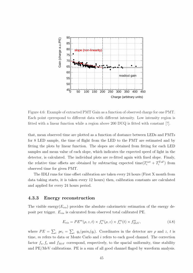
Charge (arbitrary units)
0 50 100 150 200 250 300 350 400 450
Gai
n (c
harg
e a.
u./P
E)
45
50
55
60
65
70
75
80
85
90
readout gain
slope (non-linearity)slope (non-linearity)
Figure 4.6: Example of extracted PMT Gain as a function of observed charge for one PMT.
Each point cprrespond to different data with different intensity. Low intensity region is
fitted with a linear function while a region above 200 DUQ is fitted with constant [?].
that, mean observed time are plotted as a function of dostance between LEDs and PMTs
for 8 LED sample, the time of flight from the LED to the PMT are estimated and by
fitting the plots by linear function. The slopes are obtained from fitting for each LED
samples and mean value of each slope, which indicates the expected speed of light in the
detector, is calculated. The individual plots are re-fitted again with fixed slope. Finaly,
the relative time offsets are obtained by subtracting expected time(T exti + T ToF
i ) from
observed time for given PMT.
The IDLI runs for time offset calibration are taken every 24 hours (First X month from
data taking starts, it is taken every 12 hours) then, calibration constants are calculated
and applied for every 24 hours period.
4.3.3 Energy reconstruction
The visible energy(Evis) provides the absolute calorimetric estimation of the energy de-
posit per trigger. Evis is calcurated from observed total calibrated PE.
Evis = PEm(ρ, z, t)× fmu (ρ, z)× fm
s (t)× fmMeV , (4.8)
where PE =∑
i pei =∑
i qi/gaini(qi). Coordinates in the detector are ρ and z, t is
time, m refers to data or Monte Carlo and i refers to each good channel. The correction
factor fu, fs and fMeV correspond, respectively, to the spacial uniformity, time stability
and PE/MeV calibrations. PE is a sum of all good channel flaged by waveform analysis.
45

Figure 4.7: Left : Distribution of pulse observed time from external trigger. Right :
Observed time distribution as a function of distance between LED ans PMT.(Abe-kun ni
kireina plot wo morau)
Few channels are flagged not good sporadically and are excluded from the visible energy
calculation. Four stages of calibration are carried out to render Evis. Absolute energy
scale factor fmMeV is determined usong 252Cf source deployed at detector center. Neutrons
emitted from 252Cf source are captured by hydrogen and several number of γ-rays are
emitted. Then, PE/MeV factor is obtained by matching this peak to 2.223MeV energy
deposit. The absolute energy scale are found to be 229.9 PE/MeV and 227.7 PE/MeV
for the data and MC respectively. Each step for correction factor is described in next
paragraph.
Non-uniformity correction
The PE responce is position dependent for both MC and data due to several factors such
as; acceptance of PMTs, detector structure non-uniformity (chimney, acrylic vessel and
its support structure) and difference of attenuation length of liquid in different region.
Detector responce map is applied to cancel the PE bias depending on the interaction
vetex position in the detector. The capture peak on H of neutrons from spallation and
antibutrino interactions provides, for data and for MC respectively, a precise and copious
calibration souorce to charactarize the response non-uniformity over full volume. Correc-
tion factor is defined as fractional responce for each position with respect to the detector
center.
fmu (ρ, z) =
PEmHcapture(0, 0)
PEmHcapture(ρ, z)
. (4.9)
46

Figure 4.8 is the detector responce map applied to data. A 2D-interpolation method was
developed to provide a smooth application of the calibration map at any point (ρ, z).
(m)ρ0 0.2 0.4 0.6 0.8 1 1.2 1.4 1.6 1.8 2
z (m
)
-2
-1.5
-1
-0.5
0
0.5
1
1.5
2
0.84
0.86
0.88
0.9
0.92
0.94
0.96
0.98
1
Target
GC
Figure 4.8: Detector responce map, in cylindrical coordinates(ρ, z) as sampled with spal-
lation neutrons capturing in H across the ID. Responce variations are quantified as the
fractional responce with respect to the detector center. Largest deviation in ν-target are
up to 5%. (Bernd ni MC plot wo moratte naraberu)
Syatematic uncertainty relative to MC is estimated using Gd-captured events. After
the Non-uniformity correction, detector responce map is recomputed using Gd-captured
events and the relative difference between each detector map is defined as
2× EMCi − Edata
i
EMCi + EData
i
, (4.10)
where i is a bin number of the detector map. The RMS deviation of the relative difference
distribution is used as the estimator of the non-uniformity systematic uncertainty, and is
0.43%.
Stability correction
The detector responce was found to vary in time due to two effects, which are accounted
for and corrected by the term fms (t). First, the detector responce can change due to
variation in readout gain or scintillator responce. This effect has been observed as a +2.2%
monotonic increase over 1 year using the responce of the spalaltion neutrons capturing
on Gd within the ν-target, shown in Fig 4.9. Stability correction factor is defined as,
fs(t) =PEm(t0)
PEm(t). (4.11)
47

where t0 is defined as the day of the first Cf source deployment, during August 2011. This
factor is applied to only data since MC is stable.
Elapsed Days0 50 100 150 200 250 300
Ene
rgy
Dev
iatio
n (%
)
-5-4-3-2-1012345
Pea
k en
ergy
(M
eV)
7.6
7.8
8
8.2
Figure 4.9: Time evolution of Gd captured peak position.
After the stability correction using Gd-capture peaks, H-capture peak shows remaining
instability. Systematc uncertainty in stability correction is estimated from flactuation of
H-capture peak from soalation neutrons shown Fig 4.10. RMS in distribution of relative
energy variation is defined as instability syatematics and the value is 0.61%.
Elapsed day0 50 100 150 200 250 300
Ene
rgy
devi
atio
n [%
]
-5-4-3-2-1012345
Pea
k en
ergy
[MeV
]
2.15
2.2
2.25
2.3
Energy variation (%)-4 -3 -2 -1 0 1 2 3 4
Ent
ries
/ 5 d
ays
0
2
4
6
8
10
12
14
16 Mean : -0.349
RMS : 0.606
Figure 4.10: Stability of the reconstructed energy as sampled by the evolution in responce
of the spallation neutron H-capture after Gd stability correction. Left:Time evolution
plot. Right: 1-D projection histogram. Systematics in tability correction is estimated
from RMS deviation of right histogram.
48

Non linearity systematics
After the all energy correction, data/MC discrepancies in the absolute energy scale can
still arise from the relative non-linearity across the prompt energy spectrum. This possi-
bility was explored by using all calibration sources in the energy range 0.7 - 8 MeV with
deployments along the z-axis and guide tube. Some relative non-linearity was observed (¡
0.2% / MeV) but the pattern diminished when integrated over the fill volume. A 0.85%
variation consistent with this non-linearity was measured with the z-axis calibration sys-
tem, and this is used as the systematic uncertainty for relative non-linearity. Systematic
uncertainties in energy scale are summarised in Table 4.1.
Error (%)
Relative Non-Uniformity 0.43
Relative Instability 0.61
Relative Non-Linearity 0.85
Total 1.13
Table 4.1: Systematic uncertainties on energy scale.
4.4 Muon track reconstruction
Muon tracks are reconstructed by different algorithm from point like events. Several
methods using information from the different detector are deveropped.
4.4.1 ID muon reconstruction
Muon reconstruction algorithm based on ID information is deveropped by Hamburg uni-
versity. The muon track is reconstructed by PMT hit timing assuming straight trajectory
inside the detector and spherical light fronts emitted along the muon track. Maximum
likelihood method determins most probabli tracks and outputs muon entry point(θin, φin)
and exit point(θout, φout). This algorithm requires the muon passes at least γ-catcher
volume and deposit large energy. Therefore, buffer or IV clipping muon caould not be
reconstructed by this algorithm and need to rely on other reconstruction method. Figure
4.11 shows reconstruction performance using OV hit information as a reference.
4.4.2 IV muon reconstruction
Another reconstruction algorithm using only IV information reconstruct muons more
higher efficiency. Even OV or IV clipping muons can be reconstructed. The method
49
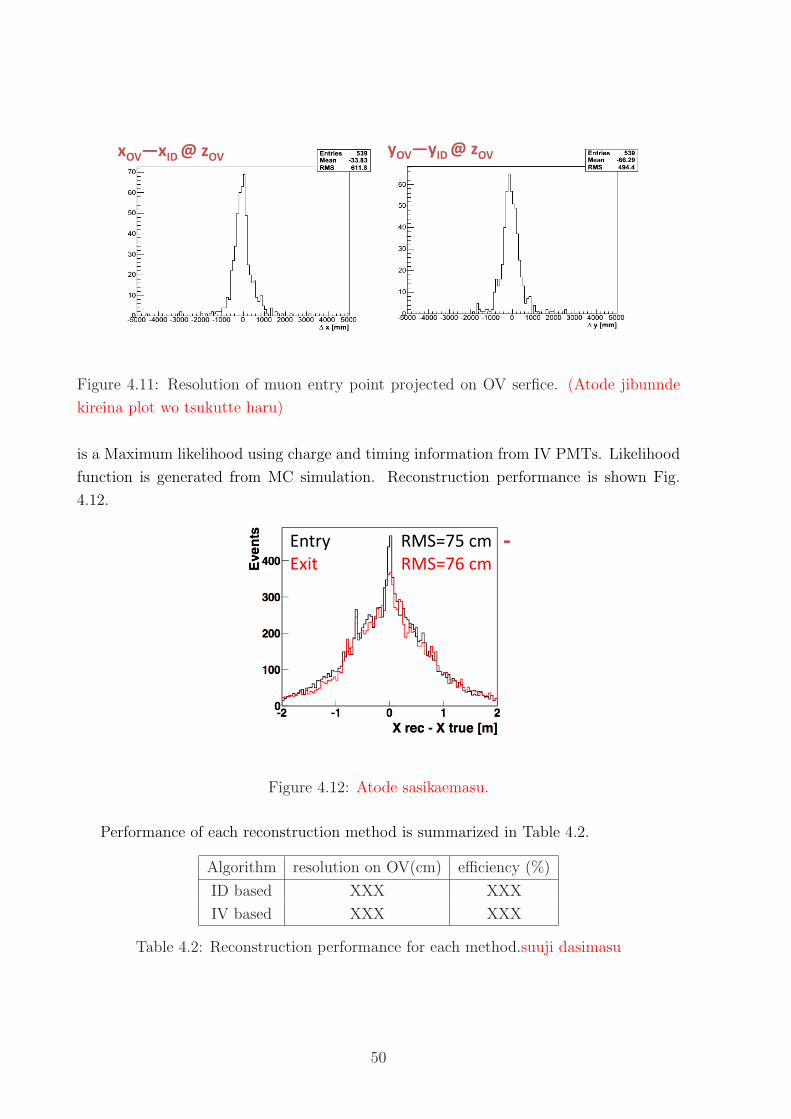
FDEGF*+,>,HDE, IDEGI*+,>,HDE,
Figure 4.11: Resolution of muon entry point projected on OV serfice. (Atode jibunnde
kireina plot wo tsukutte haru)
is a Maximum likelihood using charge and timing information from IV PMTs. Likelihood
function is generated from MC simulation. Reconstruction performance is shown Fig.
4.12.
K*5/+(
K:$5
P>QRNH(70(
P>QRNS(70
Figure 4.12: Atode sasikaemasu.
Performance of each reconstruction method is summarized in Table 4.2.
Algorithm resolution on OV(cm) efficiency (%)
ID based XXX XXX
IV based XXX XXX
Table 4.2: Reconstruction performance for each method.suuji dasimasu
50

Chapter 5
Monte Carlo simulation
5.1 Electron anti-neutrino generation
5.2 Detector simulation
5.3 Readout system simulation
51

52
Chapter 6
Selection of neutrino candidates
In order to select neutrino candidates, we require the delayed coincidence, which satisfies
two signals (prompt and delayed) and the time correlation. Derivation of θ13 is performed
by comparing data and MC spectrum. Hence, the discrepancy between data and MC
becomes mandatory parameter for oscillation analysis as described in Chap. 8. The selec-
tion efficiency and those systematic uncertainties were estimated using calibration source
data.
6.1 Strategy for neutrino selection
The event characteristics of neutrino interactions by the inverse beta decay are two in-
dependent signals by a positron and a neutron, respectively, and the time correlation
between those. As presented in Sec. 3.1, selection criteria are based on the following
requirements:
• Energy of prompt signal is to be produced by neutron energy and positron annihi-
lation,
• Energy of delayed signal is to be 8 MeV from neutron capture on Gd.
• Time correlation is to be 30 µs in average.
For event selection, we veto all signals within 1 ms after a muon, since many un-
expected effects occur. Moreover, additional cuts to reduce backgrounds, such as light
emitted by PMT itself, are required. The selection criteria based on these characteristics
are described in the Sec. 6.4.
53

6.2 Data sample
Double Chooz started the official data taking in April 2011. Figure 6.1 shows the data
taking history since data taking start. The data sample collected with the Double Chooz
far detector during the period from April 2011 to March 2012 are used in this thesis. The
total amount of run time is 251.27 days, as shown in Tab. 6.1. For a few weeks in August
to September 2011, the radioactive source data were taken for the detector calibration,
so that the corresponding runs in this period were excluded from the neutrino analysis.
Moreover, data with different configrations for several detector studies, such as PMT noise
test, were not used. In addition, the data sets are limited to those in which the electronics
have been operating properly. In the beginning of September 2011, one PMT produced
the PMT noise with high rate, and we turned off the HV for the PMT. Data with the
high rate noise before turning off HV were also removed from the analysis.
Double Chooz catches neutrino from two reactors only. Both reactors sometimes are
down for the mentainance. This oppotunity gives us to estimate backgrounds purely, by
assuming no neutrino signal. During the period used in this thesis, there were twice of
such a chance, which corresponds to Oct 2011 and May-June 2012. The backgground
analysis using such a data set is described in Chap. 7.
2011Jul.
2011Oct.
2012Jan.
2012Apr.
Dat
a ta
kin
g t
ime
(day
s)
0
50
100
150
200
250
300
350
Dat
a ta
kin
g e
ffic
ien
cy
0
0.2
0.4
0.6
0.8
1
2011Jul.
2011Oct.
2012Jan.
2012Apr.
Dat
a ta
kin
g t
ime
(day
s)
0
50
100
150
200
250
300
350Analysed Physics Others
TotalPhysicsAnalysed
Figure 6.1: Histograms (right axis) representing data taking efficiency. Solid lines corre-
spond to integrated data taking time.
54

Run time (day) Live time (day) Live time* (day)
for ν 251.27 240.17 228.25
Rector off 7.53 7.19 6.84
Table 6.1: Run time and live time used for this analysis. Reactor-off data was used for
background study described in Chap. 7. * : after additional 9Li and OV veto were applied.
6.3 Online selection
6.3.1 Double Chooz trigger system
As briefly decribed in Sec. 3.3.4, Double Chooz trigger system consists of three trigger
boards (TB-A, TB-B, TB-IV) and one trigger master board (TMB). All PMT signals are
decoupled from the high voltage at the HV splitters. After decoupling, the PMT signals
are transmitted to the Front End Electronics (FEE) module. Up to eight PMTs are
connected to one FEE module. Signals are amplified by FEE and are sent to the FADCs
for the channel by channel. The amplification factor of the FEE out put is adopted to
the dinamic range of the FADCs and factor is apploximately 8.
On the other hand, each FEE modules provides an analogue sum of all connected
16 PMTs correspond to two FEE modules input (except for two FEE with only three
connected PMTs). Those signals are transmitted to the so-called “stretcher circuit” on the
FEE modules. The circuit integrate the incoming charge of the PMTs over a time window
of 100 ns. This time is adapted to the arrival time of photons which is determined by the
detector geometry and the decay time of the scintillator as determined from dedicated
MC simulation studies [16]. The amplitude of the group signal is proportional to the
charge seen by the connected PMTs, collected within the time window of 100 ns. The
resulting output signals from the “stretcher circuit” are transmitted continuously to the
each trigger boards. The ID PMTs grouped to each trigger boards (TB-A and TB-B)
observe the same detector volume to introduce redundancy of the system. For the IV
PMTs, each grouped 3 ∼ 6 PMTs represents a certain region of the IV volume. The
grouping of the ID and IV PMTs are shown in Fig. 6.2.
For the input of the stretcher signals, each trigger bords discriminate the amplitude of
those grouped signals and sent digital trigger signals to TMB. Schimatic diagram of the
Double Chooz read out is shown in Fig. 6.3. Trigger logic of each bords are described in
next section.
55

Figure 6.2: Left : Grouping of the ID PMTs. Red and blue PMTs are connected to each
trigegr boards A and B. Both boards observe the same volume of the detector. Right :
Schimatic drawing of the PMT grouping for the IV. There are 18 different PMT groups,
each of them monitoring a certain region of the IV.
Fan Outs
LDF
LDF
NIM
NIM
LVDS
DAQ
ID Group APMTs
ID Group B
Inner Veto
PMTs
PMTs
ExternalTrigger
FEE
FEE
FEE
FEE
FEE
VME
VME
VME
Trigger Board A
Trigger Board B
Trigger Board Veto
TriggerMasterBoard
VME
(TMB)
(calibration, ...)
Trigger System
(TB A)
(TB B)
(TB V)
Inn
er Veto
78 P
MT
s390 P
MT
s
Inn
er Detecto
r
IV
ID
1x3
12x16
1x3
1x3
12x16
18x(3 ! 6) 18x(3 ! 6)
1x3
24x8
24x8
(# x #PMTs) (# x #PMTs)
Inhibit (INH)
Clock (Clk)
(62.5 MHz)
(32 bit)
(32 bit)
TriggerWord (TW)
EventNumber (EvNo)
TB output
TB output
TB output
Inhibit (INH)
Inhibit (INH)
Inhibit (INH)
Trig Ack (TA)
Trig Ack (TA)
Trig Ack (TA)
OV DAQOV sync signal7x
Trigger signal (TR1)
Figure 6.3: Schimatic diagram of the Double Chooz read out system. FEE modules
together 16 PMTs signals and build one input signal of an ID trigger board (except for
two FEE with only three connected PMTs).
56
Trigger boards and trigger logic
For the discrimination of the stretcher signal inputs and trigger release determination,
two kind of the trigger logic are impremented which are the thresholds of the summed
all groupe signals and a multiplicity condition on the single group thresholds. In the ID
trigger board, threshold for each input is set to 0.25 MeV and discreminated.
In addition, all the 13 input signals are summed up and the four thresholds called
“prescaled, neutrino, high, very high threshold” are discreminated by the pulse height of
summed signal in every 32 ns cycle clock. The prescaled threshold is lowest threshold
which set to approximatelly 0.2 MeV that delivers a rate of 1,000/s scaled by a factor of
1/1,000. The neutrino threshold is the physics threshold of the ID with no prescale factor.
It is set to approximately 0.35 MeV well below the minimum energy of the inverse beta
decay of 1.02 MeV by which neutrinos are detected. It runs at a rate of approximately
130 Hz. The two highest thresholds are used as flags for the event classification and set to
approximately 6 MeV and 50 MeV for neutron event and muons event like, respectively.
Trigger signal is generated if one of four threshold is fired. Only for the neutrino threshold
of 0.35 MeV, at least 2 of the 13 group threshold are required to be satisfied for noise
reduction.
The IV trigger board has three threshold for summed signal so-called “prescaled, low
and high” and also has threshold for group signals. Prescaled trigger is scaled by a factor
of 1/1,000 same as that of ID. Trigger is fired if the one of trigger condition is fullfilled.
Moreover, external trigger input is impremented in the trigger master board. Fixed rate
trigger signals are generated and used for monitoring. The threshold level impremented
for each trigger boards are summrised in Tab. 6.2.
Output of each trigger boards are 8-bit digital signal represanting the information of
all sum threshold condition.
Trigger master board
Figure 6.4 shows the schematic diagram of the circuit in trigger master board. Trigger
master board recieves the output of all trigger boards including the external trigger signals
and taking following function,
• Applie scalling factor of 1/1,000 to the prescale trigger bit.
• Put the event number to the trigger.
• Combine the each output of trigger board and make Trigger Word (TW).
• Send the trigger signal to the FADC.
57

Detector Name threshold (MeV)
ID prescaled 0.2
neutrino 0.35
high 5
very high 50
group-low 0.25
group-high 0.25
IV prescaled set to 1 Hz after 1/1000
low 10
high 50
group 10/number of connected PMTs
Table 6.2: Thresholds impremented to ID and IV trigger board.
All the trigger condition of each trigger bit of each trigger boards are summarized to 32
bit TW after scalling factor is applied. If FADC recieves trigger signal, that opens 256 ns
window and records digitized waveform information in this window.
Figure 6.4: Scheme of the TMB firmware implemented in the FPGA.
58

6.3.2 Trigger efficiency estimation
Trigger efficiency must be estimated precisely since it can affect directly to the number of
observed neutrinos. As described previous section, the physics trigger threshold of ID is
set to approximately 0.35 MeV. If events which deposit energy above this threshold can
be triggered perfectlly, trigger efficiency as a function of energy should be step function
ideally. However, it is ideal case but efficiency curve is observed due to resolution of
electronics. The main goal of this study that we have to determine is the trigger efficiency
at the neutrino selection energy range of 0.7 < Eprompt <12.2 MeV (Next section).
The efficiency of the neutrino threshold is estimated using prescaled trigger event
sample as,
εIDNeutrino =
Nprescaled ∧NNeutrino
Nprescaled
. (6.1)
where, denominator correspond to the number of events which prescaled trigger is fired
and numerator is the number of events which neutrino and prescaled trigger are fired.
Unfortunatelly, the problem is found in the event classification due to wideness of the
pulse rise time.
Figure 6.5 shows the trigger descrimination for the wide strecher pulse. Trigger condi-
tion is determined every 32 ns clock cycle. In Fig. 6.5, low and high threshold are fulfilled
at trigger release time. Then, once the trigger condition fulfilled, dead time of 128 ns
is produced and very high threshold could not be fired in spite of signal is larger than
threshold. This problem is occure if stretcher pulse has wide rise time. In fact, due to
the timing of the scintillator, diffrent transit times of the PMTs, the shape of the PMT
pulses and the stretcher time of 100 ns, the corresponding sum stretcher signals have a rise
time in the order of a clock cycle. This effect cause wrong event classication for neutrino
threshold if prescaled threshold is fulfilled before.
In order to solve this problem, trigger efficiency is firstry evaluated as a function of
the amplitude of stretcher signals at the trigger release time. After that, amplitude of
stretcher signals are converted to the energy. Correction factor is obtained by fitting the
distribution of energy vs stretcher amplitude.
6.3.3 Systrematic uncertainty
We considered several systematic uncertainties on the trigger efficiency explained following
section.
59

32 ns 32 ns 32 nst
ID neutrino−like thresholdID neutron−like threshold
ID muon−like threshold
ID stretcher signal
32 ns
trigger condition fulfilled
clock cycles
threshold - lowthreshold - high
threshold - very high
trigger release timeDead time for ns
Could not be fulÞlled
Figure 6.5: Schimatic example of trigger threshold discrimination.
energy [MeV*t]0 0.2 0.4 0.6 0.8 1 1.2 1.4
ma
x s
tre
tch
er
am
plitu
de (
TB
A +
TB
B)
[DU
I]
0
50
100
150
200
250
300
350
400
1
10
210
Figure 6.6: Observed charge sum vs stretcher signal amplitude.
6.4 Offline selection
Neutrino candidates are selected by following three steps. Firstly, several cuts are applied
to ensure the data quality.
• Muon veto : Reject all triggers within 1 ms from muon events. Muon events : EIV
> 5 MeV or EID > 30 MeV.
60

Figure 6.7: Errors on trigger efficiency as a function of energy. Left : Errors on upper
side. Right : Errors on lower side.
energy [MeV]0.2 0.4 0.6 0.8 1.0 1.2 1.4
trig
ger
eff
icie
ncy
0.0
0.2
0.4
0.6
0.8
1.0
Figure 6.8: .
• Noise rejection : Signals to be Qmax/Qtotal > 0.09, RMSTstart > 40 ns is rejected for
light noise (sec. 6.4.2).
• Artificial trigger rejection : Reject signals taken by external trigger.
The signals which pass those cuts are defined as “Valid triggers”. Secondly, the delayed
coincidence is required to Valid triggers for neutrino event selection as following:
• Prompt energy : 0.7 < Eprompt < 12.2 MeV in the ID.
• Delayed energy : 6 < Edelayed < 12MeV in the ID, Qmax/Qtotal < 0.055.
• ∆ T : 2 µs< ∆T < 100 µs
• Multiplicity cut : No valid trigger in [Tp− 100;Tp + 400]µs but prompt and delayed
signals.
61

In addition, following cuts for background reduction are required.
• Additional 9Li veto : Reject all events within 500 ms from high energy muon events.
High energy muon : EID >600 MeV.
• OV coincidence veto : No OV trigger coincidence to prompt signal.
The details and motivation of each cut, are described in the following section.
6.4.1 Muon veto
Cosmic muon can produce spallation neutron or radioactive isotopes by interacting with
nuclei in the detector or surrounding rock. Those spallation products can mimic prompt
or delayed signals moreover both of them by only itself. One example of such a coinci-
dence background is so-called fast neutron background describing in 7.2. In addition, as
described in Sec. 4.1, the baseline of electronics can be fluctuated after the large energy
deposit by muons. Hence, all triggers within 1ms after muon events are vetoed from anal-
ysis. Muon tagging is performed by ID and IV information respectively. Energy deposit
> 30MeV is selected as ID muon tagging and EIV > 5 MeV is applied for IV tagging.
Inner veto Muon tagging
Muon tagging using IV is performed by evaluating observed charge from IV. Tagging
efficiency is estimated using ID triggered event sample with higher energy deposit more
than 50 MeV since such large energy events must be muon and should be coming passing
though IV detector. Figure 6.9 shows a distribution of observed IV charge and estimated
muon tagging efficiency as a function of IV charge. For the neutrino selection, 10,000
DUQ threshold is used for muon tagging with over 99.8 % tagging efficiency.
Inner detector Muon tagging
What causes inefficiency of IV detector is muons which come from chimney hence do
not pass trough IV. Such muons could not identified by IV however should deposit large
energy in ID. ID muon tagging threshold of 30 MeV is adopted for neutrino selection.
Nonetheless, muons came from chimney and do not across the detector but stop at top of
detector are observed as low energy event. This kind of muon is difficult to identify and
cause so-called Stopping muon background (sec. 7.2).
Veto time
Main background source from cosmic muon is spallation neutron which can produce 8
MeV delayed like event after captured by Gd. Otherwise, captured by hydrogen and
62
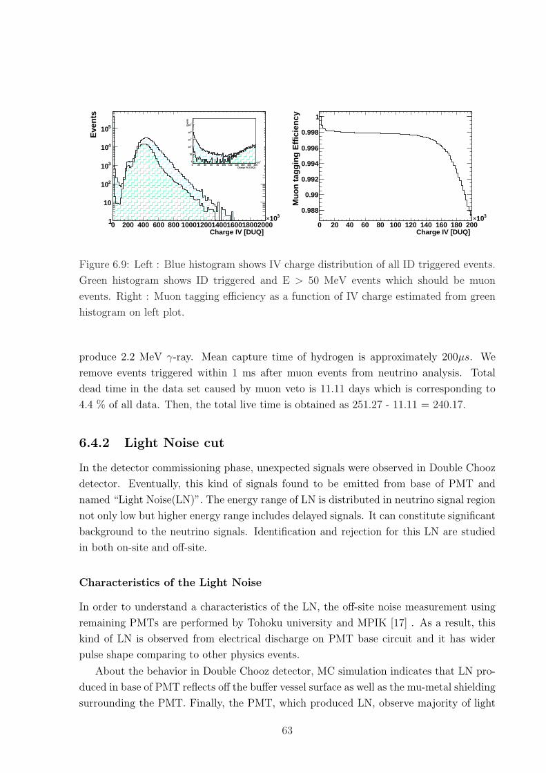
Charge IV [DUQ] 0 200 400 600 800 100012001400160018002000
310×
Eve
nts
1
10
210
310
410
510
Charge IV [DUQ] 0 20 40 60 80 100 120 140 160 180 200
310×
Eve
nts
1
10
210
310
410
510
Charge IV [DUQ] 0 20 40 60 80 100 120 140 160 180 200
310×
Mu
on
tag
gin
g E
ffic
ien
cy
0.988
0.99
0.992
0.994
0.996
0.998
1
Figure 6.9: Left : Blue histogram shows IV charge distribution of all ID triggered events.
Green histogram shows ID triggered and E > 50 MeV events which should be muon
events. Right : Muon tagging efficiency as a function of IV charge estimated from green
histogram on left plot.
produce 2.2 MeV γ-ray. Mean capture time of hydrogen is approximately 200µs. We
remove events triggered within 1 ms after muon events from neutrino analysis. Total
dead time in the data set caused by muon veto is 11.11 days which is corresponding to
4.4 % of all data. Then, the total live time is obtained as 251.27 - 11.11 = 240.17.
6.4.2 Light Noise cut
In the detector commissioning phase, unexpected signals were observed in Double Chooz
detector. Eventually, this kind of signals found to be emitted from base of PMT and
named “Light Noise(LN)”. The energy range of LN is distributed in neutrino signal region
not only low but higher energy range includes delayed signals. It can constitute significant
background to the neutrino signals. Identification and rejection for this LN are studied
in both on-site and off-site.
Characteristics of the Light Noise
In order to understand a characteristics of the LN, the off-site noise measurement using
remaining PMTs are performed by Tohoku university and MPIK [17] . As a result, this
kind of LN is observed from electrical discharge on PMT base circuit and it has wider
pulse shape comparing to other physics events.
About the behavior in Double Chooz detector, MC simulation indicates that LN pro-
duced in base of PMT reflects off the buffer vessel surface as well as the mu-metal shielding
surrounding the PMT. Finally, the PMT, which produced LN, observe majority of light
63
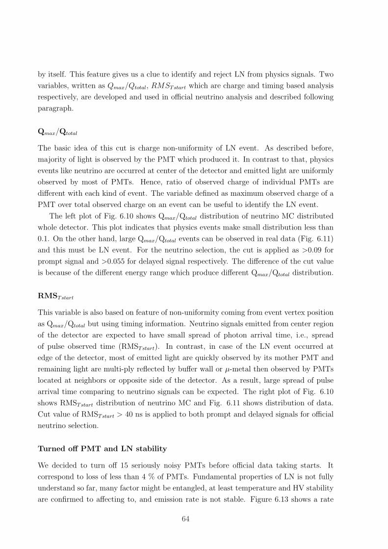
by itself. This feature gives us a clue to identify and reject LN from physics signals. Two
variables, written as Qmax/Qtotal, RMSTstart which are charge and timing based analysis
respectively, are developed and used in official neutrino analysis and described following
paragraph.
Qmax/Qtotal
The basic idea of this cut is charge non-uniformity of LN event. As described before,
majority of light is observed by the PMT which produced it. In contrast to that, physics
events like neutrino are occurred at center of the detector and emitted light are uniformly
observed by most of PMTs. Hence, ratio of observed charge of individual PMTs are
different with each kind of event. The variable defined as maximum observed charge of a
PMT over total observed charge on an event can be useful to identify the LN event.
The left plot of Fig. 6.10 shows Qmax/Qtotal distribution of neutrino MC distributed
whole detector. This plot indicates that physics events make small distribution less than
0.1. On the other hand, large Qmax/Qtotal events can be observed in real data (Fig. 6.11)
and this must be LN event. For the neutrino selection, the cut is applied as >0.09 for
prompt signal and >0.055 for delayed signal respectively. The difference of the cut value
is because of the different energy range which produce different Qmax/Qtotal distribution.
RMSTstart
This variable is also based on feature of non-uniformity coming from event vertex position
as Qmax/Qtotal but using timing information. Neutrino signals emitted from center region
of the detector are expected to have small spread of photon arrival time, i.e., spread
of pulse observed time (RMSTstart). In contrast, in case of the LN event occurred at
edge of the detector, most of emitted light are quickly observed by its mother PMT and
remaining light are multi-ply reflected by buffer wall or µ-metal then observed by PMTs
located at neighbors or opposite side of the detector. As a result, large spread of pulse
arrival time comparing to neutrino signals can be expected. The right plot of Fig. 6.10
shows RMSTstart distribution of neutrino MC and Fig. 6.11 shows distribution of data.
Cut value of RMSTstart > 40 ns is applied to both prompt and delayed signals for official
neutrino selection.
Turned off PMT and LN stability
We decided to turn off 15 seriously noisy PMTs before official data taking starts. It
correspond to loss of less than 4 % of PMTs. Fundamental properties of LN is not fully
understand so far, many factor might be entangled, at least temperature and HV stability
are confirmed to affecting to, and emission rate is not stable. Figure 6.13 shows a rate
64

total / QmaxQ0 0.02 0.04 0.06 0.08 0.1
Eve
nts
1
10
210
310
Prompt signal
Delayed signal
TstartRMS0 10 20 30 40 50 60 70 80 90 100
Eve
nts
1
10
210
310
410Prompt signal
Delayed signal
Figure 6.10: Distribution of Light Noise cut variables for Neutrino Monte Carlo. Left
: Distribution of Qmax/Qtotal for prompt (blue) and delayed (green) signals. Right :
RMSTstart distribution.
tot/QmaxQ
0.00 0.05 0.10 0.15 0.20 0.25 0.30
RM
S(T
sta
rt)
[ns]
0
10
20
30
40
50
60
70
80
Preliminary
-610
-510
-410
Preliminary
Figure 6.11: RMSTstart vs Qmax/Qtotal for gamma and neutron source calibration data
deployed along the central axis of the target. The red lines indicate the light noise cuts
used for the prompt event in the neutrino selection [18].
stability plot since data taking started. This instability is taken into account to accidental
background estimation.
65
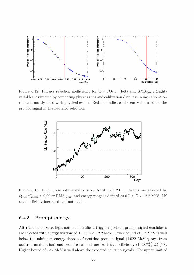
tot/QmaxQ
0.00 0.02 0.04 0.06 0.08 0.10 0.12 0.14 0.16
Ph
ys
ics
Re
jec
tio
n I
ne
ffic
ien
cy
-310
-210
-110
1
RMS(Tstart) [ns]
0 10 20 30 40 50
Ph
ys
ics
Re
jec
tio
n I
ne
ffic
ien
cy
-310
-210
-110
1
Figure 6.12: Physics rejection inefficiency for Qmax/Qtotal (left) and RMSTstart (right)
variables, estimated by comparing physics runs and calibration data, assuming calibration
runs are mostly filled with physical events. Red line indicates the cut value used for the
prompt signal in the neutrino selection.
Days0 100 200 300
Lig
ht-
no
ise
Ra
te [
Hz]
15
20
25
Figure 6.13: Light noise rate stability since April 13th 2011. Events are selected by
Qmax/Qtotal > 0.09 or RMSTstart and energy range is defined as 0.7 < E < 12.2 MeV. LN
rate is slightly increased and not stable.
6.4.3 Prompt energy
After the muon veto, light noise and artificial trigger rejection, prompt signal candidates
are selected with energy window of 0.7 < E < 12.2 MeV. Lower bound of 0.7 MeV is well
below the minimum energy deposit of neutrino prompt signal (1.022 MeV γ-rays from
positron annihilation) and promised almost perfect trigger efficiency (100.0+0.0−0.1 %) [19].
Higher bound of 12.2 MeV is well above the expected neutrino signals. The upper limit of
66

expected energy deposit from neutrino event is ∼8 MeV, hence events in an energy range
of 9 < E < 12.2 MeV are background dominant. However, events in this higher energy
region can be useful to constrain the background signals at low energy region when the
final fitting will perform.
6.4.4 Delayed energy
Delayed signal candidates are chosen with energy window of 6 < E < 12 MeV and tighter
light noise cut of Qmax/Qtotal. The presence of a gamma catcher ensures that the energy
from neutron capture events on Gd is fully absorbed most of the time. However, the
delayed event neutron capture on Gd visible energy distribution for neutrino candidates
has a tail that extends down to energies of 5 MeV and below. The lower limit of the
delayed energy window was chosen to be a relatively flat part of the energy spectrum
with relatively good agreement between data and MC (see Sec. ). The upper limit of the
delayed energy window was conservatively chosen to be 12 MeV. This is well above the
full absorption peak of neutron capture on Gadolinium and has negligible inefficiency for
neutrino selection.
6.4.5 DeltaT
Neutrons produced from inverse beta decay are thermalized by proton scattering in the
detector and finally captured by Gd or Hydrogen. Mean captured time on Gd is ap-
proximately 30 µs. Time coincidence between prompt and delayed signal candidate are
selected as 2 < ∆ T< 100µs. Upper limit is over three times larger than expected mean
capture time on Gd. Lower limit is selected to eliminate background contamination such
as light noise or stopping muon. Moreover, uncertainty related to neutron thermalization
model in lower ∆T region is also can be suppressed.
6.4.6 Multiplicity cut
Finally, multiplicity cut is applied to remove correlated background. This cut requires no
varied trigger events existing in 100 µs proceeding to prompt event and 400 µs following
prompt event except for only one delayed event candidate. Varied trigger event is defined
as E > 0.5 MeV after the muon veto, light noise and artificial trigger rejection.
Schematic image of neutrino selection is shown in Fig. 6.14.
6.4.7 Additional 9Li veto
Cosmogenic 9Li background is largest background in Double Chooz detector. 9Li isotope
is produced from spallation interaction by very high energy muon with 12C. Such a high
67

Prompt signal0.7 < E < 12.2 MeV
2~100!s from prompt
time
No other trigger in [Tp - 100 ; Tp + 400 !s]
Neutrino selection
Multiplicity cut
"T
Delayed signal6 < E < 12 MeV
Figure 6.14: Schismatic image of neutrino selection.
energy muon is no longer a MIP but deposit huge energy in the detector. Moreover,
it produce a lot of spallation products not only 9Li but mainly neutron and so-called
showering muon. We apply additional longer muon veto for 9Li background reduction.
That is, reject all events within 500 ms from showering muon events. Showering muon is
defined by : EIDµ >600 MeV.
E vs track length no Plot haru.
6.4.8 OV coincidence veto
No OV signal coincidence is required for prompt signal for cosmogenic correlated back-
ground rejection. OV coincidence is defined as 224 ns proceeding to prompt signal. Trigger
rate of OV is ∼ 2.7 kHz, hence dead time produced by this cut is 0.062 %.
6.4.9 Neutrino selection summary and MC comparison
In summary for neutrino selection, several control plots are shown in this section. In
the standard neutrino selection (no additional 9Li veto and OV veto), 9021 neutrino
candidate events are found in 251.27 days data. It becomes 8347 and 8249 candidates
after additional 9Li veto and OV veto is applied. Following plots contain 9021 candidates
selected by standard neutrino selection. Neutrino Monte Carlo sample of no-oscillation
hypothesis (no background events) are superimposed in each plot.
The delayed energy distribution is shown in Fig. 6.16. A few percents of shift can
be seen in the distribution. This discrepancy is considered in the extraction of θ13 in the
energy spectrum fitting. Figure 6.17 and Fig. 6.18 shows Delta T and Delta R distribution,
respectively. They are in good agreement between data and MC, except for high ∆R
due to no background in MC. Moreover, distributions of Qmax/Qtotal and RMSTstart are
68

plotted in Fig. 6.19 and 6.20, respectively. Qmax/Qtotal distribution shows good agreement
and background events of higher Qmax/Qtotal can be seen.
Standard + 9Li veto + OV veto
Run Time (days) 251.27 251.27 251.27
Veto time (days) 11.11 (4.4%) 23.02 (9.2 %) 23.11 (9.2 %)
Live time (days) 240.17 228.25 228.16
νe candidates 9021 8347 8249
Table 6.3: Neutrino selection summary.
Prompt E (MeV)0 2 4 6 8 10 12 14
Del
ayed
E (
MeV
)
0
2
4
6
8
10
12
14
Figure 6.15: Correlation between prompt and delayed event candidate. Red line indicates
selected neutrino candidates.
69

Delayed Energy (MeV)6 7 8 9 10 11 12
Eve
nts
/ 0.
25 M
eV
0
500
1000
1500
2000
2500
DATA
MC
Figure 6.16: Delayed energy distribution of selected neutrino candidate events.
s)µDelta T (0 10 20 30 40 50 60 70 80 90 100
sµE
ven
ts /
2
10
210
310
DATA
MC
Figure 6.17: Delta T distribution
70

R (cm)∆0 50 100 150 200 250
Eve
nts
/ 5 c
m
-210
-110
1
10
210
310DATA
MC
Figure 6.18: Distance between prompt and delayed signal reconstructed position.
total / Q
maxPrompt Q
0 0.02 0.04 0.06 0.08 0.1
Eve
nts
-210
-110
1
10
210
310DATA
MC
total / Q
maxDelayed Q
0 0.02 0.04 0.06 0.08 0.1
Eve
nts
-210
-110
1
10
210
310DATA
MC
Figure 6.19: Distribution of Qmax/Qtotal for Prompt (left) and Delayed (right) signal.
71

(ns)Tstart
Prompt RMS0 5 10 15 20 25 30 35 40 45 50
Eve
nts
/ ns
-210
-110
1
10
210
310
DATA
MC
(ns)Tstart
Delayed RMS0 5 10 15 20 25 30 35 40 45 50
Eve
nts
/ ns
-110
1
10
210
310DATA
MC
Figure 6.20: Distribution of RMSTstart for Prompt (left) Delayed (right) signal.
)2 (m2ρPrompt 0 0.5 1 1.5 2 2.5
2E
ven
ts /
500
cm
0
100
200
300
400
500DATA
MC
)2 (m2ρDelayed 0 0.5 1 1.5 2 2.5
2E
ven
ts /
500
cm
0
100
200
300
400
500DATA
MC
Figure 6.21: Vertex distribution of ρ for Prompt (left) and Delayed (right) signal.
72

Prompt Z (m)-2.5 -2 -1.5 -1 -0.5 0 0.5 1 1.5 2 2.5
Eve
nts
/ 10
cm
0
100
200
300
400
500
600
DATA
MC
Delayed Z (m)-2.5 -2 -1.5 -1 -0.5 0 0.5 1 1.5 2 2.5
Eve
nts
/ 10
cm0
100
200
300
400
500
600
DATA
MC
Figure 6.22: Vertex distribution of Z for Prompt (left) and Delayed (right) signal.
X position (m)-2 -1.5 -1 -0.5 0 0.5 1 1.5 2
Y p
ositi
on (
m)
-2
-1.5
-1
-0.5
0
0.5
1
1.5
2
0
5
10
15
20
25-targetν
-catcherγ
X position (m)-2 -1.5 -1 -0.5 0 0.5 1 1.5 2
Y p
ositi
on (
m)
-2
-1.5
-1
-0.5
0
0.5
1
1.5
2
0
5
10
15
20
25
30
35-targetν
-catcherγ
Figure 6.23: Vertex distribution of X-Y plane for Prompt (left) and Delayed Signal.
73
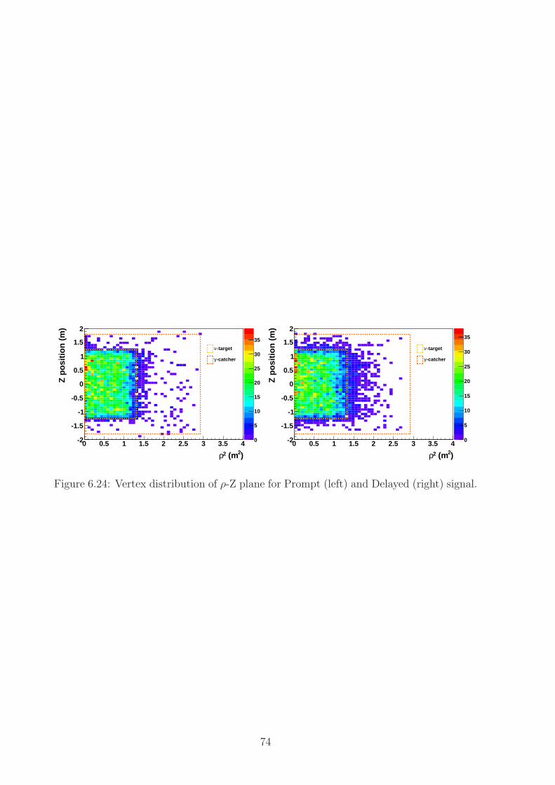
)2 (m2ρ0 0.5 1 1.5 2 2.5 3 3.5 4
Z p
ositi
on (
m)
-2
-1.5
-1
-0.5
0
0.5
1
1.5
2
0
5
10
15
20
25
30
35
-targetν
-catcherγ
)2 (m2ρ0 0.5 1 1.5 2 2.5 3 3.5 4
Z p
ositi
on (
m)
-2
-1.5
-1
-0.5
0
0.5
1
1.5
2
0
5
10
15
20
25
30
35
-targetν
-catcherγ
Figure 6.24: Vertex distribution of ρ-Z plane for Prompt (left) and Delayed (right) signal.
74

6.5 Estimation of selection efficiencies and systemat-
ics
6.5.1 Neutron detection efficiency and systematics
Discrepancy between data and MC in neutrino selection is mainly coming from neutron
thermalization model and capture fraction of Gd and hydrogen. The estimation of the cut
efficiency and systematic check is studied using 252Cf source deployment data and tuned
MC. The neutron detection efficiency εneutron consists of three efficiency components and
defined as,
εneutron = εGd × ε∆T × εE, (6.2)
where, εGd is the fraction of neutron captures on gadolinium, ε∆T is the fraction of neutron
captures within desired time interval 2 < ∆T < 100µs and εE is the fraction of neutron
captures within energy range 6 < Edelayed < 12 MeV. Energy distribution of neutron
capture events obtained from 252Cf source deployment data is shown in Fig. 6.5.1 and
delta T distribution is shown Fig. 6.5.1. One can see small discrepancy between data and
MC in distribution. This relative uncertainty between data and MC must be estimated.
Visible Energy(MeV)5 10 15 20 25
Ev
en
ts(a
rb.
un
its
)
1
10
210
310
410Cf_Data
252
Cf_MC252
Normalized Delayed Signal
Figure 6.25: Energy distribution of neutron capture events from 252Cf calibra-
tion source deployment data (black) and MC (red).
Neutron capture fraction
Thermalized neutrons produced from inverse beta-decay are captured by Gd with high
cross section but some of them are captured by H. εGd is defined as a ratio of Gd capture
to total neutron emission and estimated as,
75

s]µ T from Prompt event [∆0 20 40 60 80 100 120 140 160 180 200
s]µA
rea
norm
aliz
ed r
ate
[bin
/ 2
-510
-410
-310
-210
-110
Figure 6.26: Delta T distribution of neutron capture events from 252Cf cali-
bration source deployment data (black) and MC (red).
εGd =N(Gd)
N(Gd) +N(H), (6.3)
where N(Gd) is total number of neutron captured event on Gd and N(H) is captured
on H. The number of each kind of event are calculated by fitting a capture peak. Four
peaks are observed in energy distribution composed of H capture (2.2 MeV), Gd capture
(8MeV), Gd + H double capture (12.2 MeV) and Gd + Gd double capture (16 MeV).
Other effects that could result in a loss of a neutron, such as capture on carbon and
neutron decay, are ignored as sub-dominant here. H capture peak of 2.2 MeV is fitted
by Gaussian and exponential function indicates background from low energy region. The
Gd capture peak of 8MeV consists of two Gaussian, which correspond to Gd-155 and Gd-
157 capture respectively, and an error function representing edge of compton scattering.
Example of fitting for data and MC is shown in Fig. 6.5.1.
Delta T cut efficiency
Delta T cut efficiency is defined as ratio of number of neutron capture events within
2 < ∆T < 100µs to number of neutron capture events within 0 < ∆T < 200µs.
ε∆T =N(6 < Edelayed < 12[MeV ])
N(4 < Edelayed < 12[MeV ]), (6.4)
The efficiency is calculated for each z-axis position respectively (Fig. 6.5.1). Central value
of each data sample is obtained as ε∆T = 0.9645 ± 0.0024 for data and ε∆T = 0.9692 ±0.001 for MC. Relative uncertainty between data and MC
δε =ε(data)− ε(MC)
ε(data)(6.5)
76
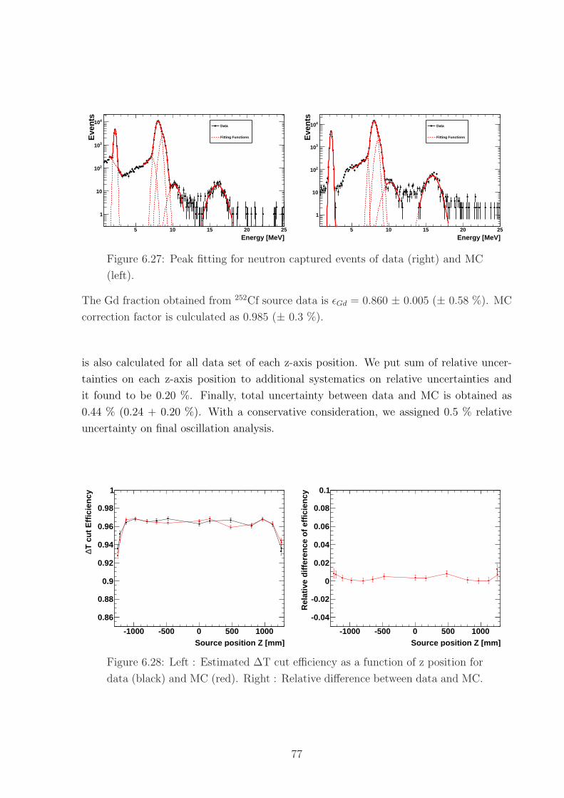
Energy [MeV]5 10 15 20 25
Eve
nts
1
10
210
310
410Data
Fitting Functions
Energy [MeV]5 10 15 20 25
Eve
nts
1
10
210
310
410 Data
Fitting Functions
Figure 6.27: Peak fitting for neutron captured events of data (right) and MC
(left).
The Gd fraction obtained from 252Cf source data is εGd = 0.860 ± 0.005 (± 0.58 %). MC
correction factor is culculated as 0.985 (± 0.3 %).
is also calculated for all data set of each z-axis position. We put sum of relative uncer-
tainties on each z-axis position to additional systematics on relative uncertainties and
it found to be 0.20 %. Finally, total uncertainty between data and MC is obtained as
0.44 % (0.24 + 0.20 %). With a conservative consideration, we assigned 0.5 % relative
uncertainty on final oscillation analysis.
Source position Z [mm]-1000 -500 0 500 1000
T c
ut E
ffici
ency
∆
0.86
0.88
0.9
0.92
0.94
0.96
0.98
1
Source position Z [mm]-1000 -500 0 500 1000
Rel
ativ
e di
ffere
nce
of e
ffici
ency
-0.04
-0.02
0
0.02
0.04
0.06
0.08
0.1
Figure 6.28: Left : Estimated ∆T cut efficiency as a function of z position for
data (black) and MC (red). Right : Relative difference between data and MC.
77

Delayed energy cut efficiency
Delayed energy cut efficiency is defined as fraction of number of event included in different
energy range,
εE =N(6 < Edelayed < 12[MeV ])
N(4 < Edelayed < 12[MeV ]), (6.6)
Calculation is performed each z-axis data sample and we got ε = 0.9643 ± 0.2%2. Same
method to estimate total uncertainty as ε∆T case is applied as well. Total uncertainty is
estimated to be 0.6 %. Systematics in neutron capture are summarized in Tab. 6.4.
Efficiency Relative uncertainty (%)
Gd fraction 0.860 ± 0.005 0.3
∆ T 0.9645 ± 0.0024 0.5
Delayed E cut 0.9640 ± 0.0022 0.6
Table 6.4: Efficiency and systematic uncertainties on neutron capture.
Multiplicity cut efficiency
The multiplicity cut introduces an inefficiency to the neutrino selection due to the random
coincidence of a trigger with E> 0.5 MeV within 100 µs before and 400 µs after the prompt
event. This inefficiency can be accurately determined from the data by measuring the
rate of triggers which satisfy the isolation cut energy threshold and multiplying by the
500 µs window. For the given time window ∆T , the probability that singles of trigger
rate R would come into the window is given by Poisson statistics:
Prob. = 1− exp(−R ·∆T ). (6.7)
The multiplicity cut efficiency for the data is found to be 99.5% with negligible uncertainty.
Therefore, the neutrino MC must be corrected to account for this inefficiency since it
contains no backgrounds.
6.5.2 Spill-in/out
Neutrino signal is recognized by coincidence of two signals, which are positron annihilation
with neutrino energy (prompt) and neutron capture (delayed) event, produced by inverse
beta-decay. Positron immediately deposit their energy and annihilate, on the other hand,
neutron randomly walk around until it will be captured, by kicking proton, in the detector.
MC simulation indicates that neutron could walk about 10 ∼ 30 cm from interaction point
of inverse beta-decay. When neutrino interaction occurs at γ-catcher volume, this event
78

could not be counted the neutrino event since neutron will captured on H. However, if
neutron wander into target volume, neutron will be captured on Gd. This kind of event
is called Spill-in. The opposite effect called Spill-out effect is also happen when neutrino
interaction occurs at target volume and neutron escape from target. Those opposite two
effect could not compensate with each other.
In fact, Spill-in effect is expected to be bit larger than Spill-out, since the capture
time of neutron on Gd (∼ 30µs) is shorter than that of on H (∼ 100µs). In addition,
the volume surrounding target acrylic vessel is also asymmetry with target and γ-catcher
volume.
This Spill-in/out effect is estimated using MC simulation. Figure 6.5.2 shows neutron
leakage around the acrylic wall. The total Spill-in/out correction factor is obtained as +
1.347 ± 0.035 %. Some MC models and conditions are varied for the systematic check.
The varied conditions are,
• Neutron thermalization model.
• Gd concentration of target scintillator.
• Hydrogen concentration of γ-catcher scintillator.
• Acrylic target vessel geometry and thickness.
Finally, the Spill-in/out correction factor is found to be + 1.347 ± 0.295 (syst.) ± 0.035
% (stat.).
Figure 6.29: Neutron detection efficiency leakage as a function of distance from
acrylic wall of the target.
Systematic uncertainties related to detector components and selection criteria is sum-
marised in 6.5.
79

MC correction factor uncertainty (%)
Muon veto 0.955 Negligible
Gd fraction 0.985 0.3
∆ T cut 1 0.5
Delayed E cut 1 0.6
Spill in/out 1 0.3
Np measurement 1 0.3
Multiplicity cut 0.995 Negligible
Trigger threshold 1 Negligible
Total 0.936 0.94
Table 6.5: MC correction factor and its systematic uncertainties to the neutrino number
related to detector and selection criteria.
80

Chapter 7
Background estimation
In Double Chooz, four kind of backgrounds are expected to contaminate neutrino selec-
tion. They are so-called Accidentals, Fast neutron, Stopping muon and 9Li/8He isotopes,
respectively. Those backgrounds should be rejected as much as possible, for example ap-
plying muon time coincidence veto, but it is impossible to eliminate them perfectly. In
this section, background estimation for Double Chooz detector is presented.
Especially, 9Li/8He isotope background is a largest background in Double Chooz and
yields largest uncertainty in neutrino energy spectrum. Estimation of 9Li background will
be described particularly in the next chapter.
7.1 Accidental background
Most of events we triggered are uncorrelated signals so-called singles, like environmen-
tal radiation γ-ray or cosmogenic spallation products coming from outside the detector.
Those singles are randomly triggered and do not make neutrino mimic signals by it selves.
However, if two singles come in 2-100 µs time window, they make neutrino like signals
and so-called Accidentals. Prompt like signals are mainly caused by radiative γ-ray from
impurities in acrylic vessels or PMT glass. Delayed like signals are created by spallation
neutron captured on Gd or 12B radioactive isotope. 12B beta decay (Q value = 13.4 MeV)
can be mimic delayed like signals but difficult to reject by muon 1 ms coincidence, because12B has longer live tome of of 29.14±0.03 [?].
The rate and shape of accidental background are estimated by off-time method. In
order to select accidental coincidence in the neutrino energy window, delayed coincidence
search same as neutrino selection but different time window are applied to all data. Time
window is defined by [ 1s+2µs, 1s + 100µs ] after prompt candidate signals. Buffer time
taken to be 1 s is long enough to remove correlated signals even long lived isotopes, thus
the coincidence signals in this separated time window are completely uncorrelated events.
81

Moreover, 198 additional off-time windows are opened at 1 s + 500×n µs (n = 0,1,...197)
after prompt event to improve statistics. By this multi off-time window method, statistical
uncertainty on estimation can be Finally less than 1 %.
In this case, multiplicity cut, described in 6.4.6, is applied to both around prompt
events and also around off-time window. Hence, we have to note that multiplicity cut is
doubly applied in this estimation. The probability that singles of trigger rate R would
come into the time window ∆T is given in sec. 6.5.1. The correction factor applied to
the obtained Accidental background is obtained as
εcorr =exp(−RTwin)
exp(−2RTwin)= 100.5% (7.1)
where R is the trigger rate of the varied trigger events and Twin is time window size of
multiplicity cut = 500 µs. Numerator represents the probability that signal coincidence
does not come in the window of Twin (Neutrino selection) and denominator is that of time
window 2Twin (off-time Accidental background selection).
Figure ?? shows prompt energy spectrum of accidental background superimposed to
scaled single spectrum. Accidental spectrum is consistent with singles spectrum. Low
energy events up to 3 MeV is produced by radiative γ-ray mainly from 232Th (Q =
2.614 MeV), 40K (Q = 1.505 MeV) and 238U (Q = 4.27 MeV α) containing the glass
of PMTs. Delta T distribution obtained from off-time method is shown in left plot of
Fig. 7.1 and the distribution is flat as expected. In the right plot of Fig. 7.1, delta R
distribution of Neutrino candidate events selected from data and MC is superimposed to
that of Accidentals. Neutrino candidate events have space correlation between prompt and
delayed signals, while delta R distribution of accidental backgrounds are widely distributed
up to 5 m and well explain large delta R region of neutrino data.
The total accidental background rate is obtained as 0.345 ± 0.003 events par day. No
systematic effect has been found moving the time window and repeating the accidental
selection 30 times. The dispersion of such 30 measurements is consistent with statistical
uncertainty only.
7.2 Fast neutron and Stopping muon
7.3 9Li and 8He isotopes
7.4 Reactor OFF analysis
82

E (MeV)0 2 4 6 8 10 12
En
trie
s / 2
00 k
eV
1
10
210
310Singles scaled
Accidental prompt
Figure 7.1: Accidental background spectrum. Black point : Prompt energy
spectrum of accidental background obtained from off-time method. Red his-
togram : Singles energy spectrum scaled to black point. The shoulders at ∼1.4 MeV and ∼ 2.6 MeV are due to decay of 40K and 208Th, respectively.
Day0 50 100 150 200 250 300
)-1
Acc
iden
tal R
ate
(day
0.1
0.15
0.2
0.25
0.3
0.35
0.4
0.45
0.5
Rate per day
Figure 7.2: Accidental event rate par day. Fluctuation is seen due to light
noise instability but almost consistent with error bar.
83

/ ndf 2χ 44 / 30Prob 0.04766p0 148.7± 545.4 p1 1.417e-07± -4.199e-08
T (ns)∆1000 1010 1020 1030 1040 1050 1060 1070 1080 1090
610×
Ent
ries
/ 3m
s
100
200
300
400
500
600
/ ndf 2χ 44 / 30Prob 0.04766p0 148.7± 545.4 p1 1.417e-07± -4.199e-08
r(mm)∆0 500 1000 1500 2000 2500 3000 3500 4000 4500 5000
-210
-110
1
10
210
310Neutrino MC
Accidental back.
IBD candidates
Figure 7.3: Left : Delta T distribution of accidental background obtained
from off-time method. Distribution is flat as expected. Right : Distance
between prompt and delayed signal for Neutrino candidate (black), Accidental
background obtained from off-time method (red) and neutrino MC (yellow).
84

Chapter 8
9Li Background estimation
8.1 9Li signal shape estimation
8.2 Muon and 9Li event Monte Carlo
8.3 Effciency estimation and Cut optimization
8.4 Systematic uncertainties
8.5 Summary and discussion
85

86

Chapter 9
Oscillation analysis
87

88

Chapter 10
Result and Discussion
89

90

Chapter 11
Conclusion
91

92

Bibliography
[1] Huber, Patrick and Schwetz, Thomas, Phys.Rev. D70 (2004) 053011.
[2] R. B. Firestone., Table of Isotopes, (1996).
[3] W. Pauli, Phys. Today 31N9 (1987) 27.
[4] Fermi, E., Z.Phys. 88 (1934) 161–177.
[5] Cowan, C.L. and Reines, F. and Harrison, F.B. and Kruse, H.W. and McGuire, A.D.,
Science 124 (1956) 103–104.
[6] Danby, G. and Gaillard, J.M. and Goulianos, Konstantin A. and Lederman, L.M.
and Mistry, Nari B. and others, Phys. Rev. Lett. 9 (1962) 36–44.
[7] Kodama, K. and others, Phys. Lett. B504 (2001) 218–224.
[8] Davis, Raymond, Jr. and Harmer, Don S. and Hoffman, Kenneth C., Phys. Rev.
Lett. 20 (1968) 1205–1209.
[9] Fukuda, Y. and others, Phys.Rev.Lett. 77 (1996) 1683–1686.
[10] Abdurashitov, J.N. and others, Phys.Rev. C60 (1999) 055801.
[11] Anselmann, P. and others, Phys.Lett. B342 (1995) 440–450.
[12] Helmer, R.L., Nucl.Phys.Proc.Suppl. 98 (2001) 157–164.
[13] Maki, Ziro and Nakagawa, Masami and Sakata, Shoichi, Prog.Theor.Phys.
28 (1962) 870–880.
[14] Fukuda, Y. and others, Phys.Rev.Lett. 81 (1998) 1562–1567.
[15] Guo, Xinheng and others (2007).
[16] Ardellier, F. and others, Double Chooz: A Search for the neutrino mixing angle
theta(13). Preprint hep-ex/0606025, (2006).
93

[17] Abe, Y. and others, Phys.Rev.Lett. 108 (2012) 131801.
[18] Glashow, S.L., Nucl.Phys. 22 (1961) 579–588.
[19] Weinberg, Steven, Phys.Rev.Lett. 19 (1967) 1264–1266.
[20] Mikheev, S.P. and Smirnov, A. Yu., Sov.J.Nucl.Phys. 42 (1985) 913–917.
[21] Bemporad, Carlo and Gratta, Giorgio and Vogel, Petr, Rev.Mod.Phys. 74 (2002) 297.
[22] Kwon, H. and Boehm, F. and Hahn, A.A. and Henrikson, H.E. and Vuilleumier, J.L.
and others, Phys.Rev. D24 (1981) 1097–1111.
[23] Achkar, B. and Aleksan, R. and Avenier, M. and Bagieu, G. and Bouchez, J. and
others, Phys.Lett. B374 (1996) 243–248.
[24] Vogel, P. and Beacom, John F., Phys.Rev. D60 (1999) 053003.
[25] Wilkinson, Denys H., Z.Phys. A348 (1994) 129–138.
[26] Wilkinson, Denys H., Nucl.Phys. A377 (1982) 474–504.
[27] An, F.P. and others, Phys.Rev.Lett. 108 (2012) 171803.
[28] Ahn, J.K. and others, Phys.Rev.Lett. 108 (2012) 191802.
[29] Mueller, Th.A. and Lhuillier, D. and Fallot, M. and Letourneau, A. and Cormon, S.
and others, Phys.Rev. C83 (2011) 054615.
[30] Schreckenbach, K. and Colvin, G. and Gelletly, W. and Von Feilitzsch, F., Phys.Lett.
B160 (1985) 325–330.
[31] H. Murayama, available on
http://hitoshi.berkeley.edu/neutrino.
[32] Cabrera, A., Nucl.Instrum.Meth. A617 (2010) 473–477.
[33] Apollonio, M. and others, Eur.Phys.J. C27 (2003) 331–374.
[34] Boehm, F. and others, Nucl.Phys.Proc.Suppl. 77 (1999) 166–170.
[35] Zbiri, Karim, Note on Drexel tests of the IMB R1408 PMTs used in the inner veto
of both far and near detectors of the Double Chooz experiment. Preprint 1104.4045,
(2011).
[36] McGrew, C. and Becker-Szendy, R. and Bratton, C.B. and Breault, J.L. and Cady,
D.R. and others, Phys.Rev. D59 (1999) 052004.
94

[37] Dietrich, D. and Greiner, D. and Jochum, J. and Lachenmaier, T. and Stokes, L.F.F.
and others, JINST 7 (2012) P08012.
[38] Maeda, J., J.Phys.Conf.Ser. 331 (2011) 022018.
[39] Matsubara, T. and Haruna, T. and Konno, T. and Endo, Y. and Bongrand, M. and
others, Nucl.Instrum.Meth. A661 (2012) 16–25.
[40] Bauer, C. and Borger, E. and Hofacker, R. and Janner, K. and Kaether, F. and
others, JINST 6 (2011) P06008.
[41] CAEN Corporation, available on
http://wwwcaen.it/.
[42] F. Sato et al., Physics Procedia 37 (2012) 1164 – 1170.
[43] T. Akiri. Thesis, (2010). Ph. D. thesis, Universite Paris-Diderot.
[44] Beissel, F. and Cabrera, A. and Cucuanes, A. and Dawson, J.V. and Kryn, D. and
others, The Trigger and Timing System of the Double Chooz Experiment. Preprint
1209.5607, (2012).
[45] P. Novella et al., DCRecoPulse, Software and algorithms for pulse reconstruction.
Double Chooz internal note: DC-doc-649-v2, 2009.
[46] I. Stancu, The Double Chooz Optical Model. Double Chooz internal note: DC-doc-
2897, 2011.
[47] S. M. Habib, Reconstruction of Events in RecoBAMA. Double Chooz internal note:
DC-doc-4331, 2012.
[48] F.J. Lombard and F. Martin, Rev. Sci. Instrum. 32 (1961) 200.
[49] Y. Abe, Linearized-PE calibration technical note. Double Chooz internal note: DC-
doc-4114-v2, 2012.
[50] A. Cucuanes. Thesis, (2009). Ph. D. thesis, RWTH Aachen University.
[51] F. Suekane, Report for the light noise. Double Chooz internal note, DC-doc-2565,
2011.
[52] D. Franco, Light-noise cut test with calibration data. Double Chooz internal note:
DC-doc-2900, 2011.
[53] A. Stueken, Trigger efficiency for 2nd pub. Double Chooz internal note: DC-doc-
3966-v2, 2012.
95

[54] Ajzenberg-Selove, F., Nucl.Phys. A506 (1990) 1–158.
96
Recommended