University of VermontScholarWorks @ UVM
Graduate College Dissertations and Theses Dissertations and Theses
2017
Microwave Bessel-Beam Propagation throughSpatially Inhomogeneous MediaRyan Francis GreccoUniversity of Vermont
Follow this and additional works at: https://scholarworks.uvm.edu/graddis
Part of the Electrical and Electronics Commons, and the Physics Commons
This Thesis is brought to you for free and open access by the Dissertations and Theses at ScholarWorks @ UVM. It has been accepted for inclusion inGraduate College Dissertations and Theses by an authorized administrator of ScholarWorks @ UVM. For more information, please [email protected].
Recommended CitationGrecco, Ryan Francis, "Microwave Bessel-Beam Propagation through Spatially Inhomogeneous Media" (2017). Graduate CollegeDissertations and Theses. 726.https://scholarworks.uvm.edu/graddis/726

Microwave Bessel-Beam Propagation
through Spatially Inhomogeneous Media
A Thesis Presented
by
Ryan F. Grecco
to
The Faculty of the Graduate College
of
The University of Vermont
In Partial Fullfillment of the Requirementsfor the Degree of Master of Science
Specializing in Electrical Engineering
May, 2017
Defense Date: September 21, 2016Thesis Examination Committee:
Kurt E. Oughstun, Ph.D., AdvisorDarren L. Hitt, Ph.D., Chairperson
Tian Xia, Ph.D.Cynthia J. Forehand, Ph.D., Dean of Graduate College
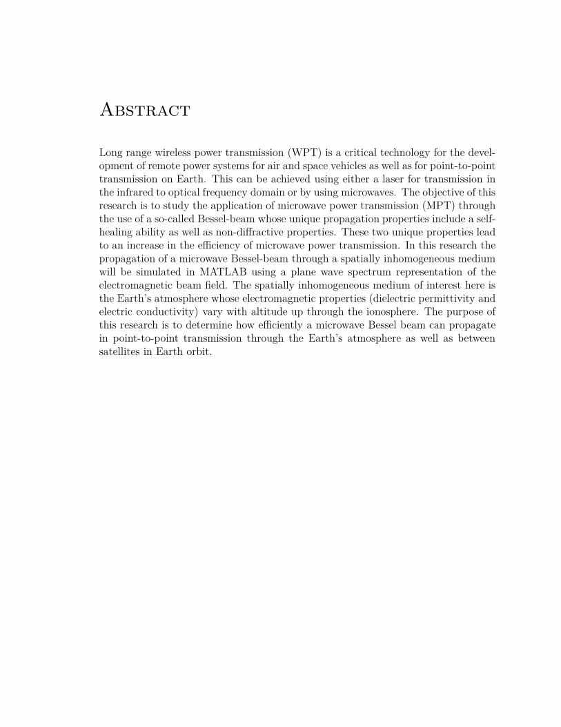
Abstract
Long range wireless power transmission (WPT) is a critical technology for the devel-opment of remote power systems for air and space vehicles as well as for point-to-pointtransmission on Earth. This can be achieved using either a laser for transmission inthe infrared to optical frequency domain or by using microwaves. The objective of thisresearch is to study the application of microwave power transmission (MPT) throughthe use of a so-called Bessel-beam whose unique propagation properties include a self-healing ability as well as non-diffractive properties. These two unique properties leadto an increase in the efficiency of microwave power transmission. In this research thepropagation of a microwave Bessel-beam through a spatially inhomogeneous mediumwill be simulated in MATLAB using a plane wave spectrum representation of theelectromagnetic beam field. The spatially inhomogeneous medium of interest here isthe Earth’s atmosphere whose electromagnetic properties (dielectric permittivity andelectric conductivity) vary with altitude up through the ionosphere. The purpose ofthis research is to determine how efficiently a microwave Bessel beam can propagatein point-to-point transmission through the Earth’s atmosphere as well as betweensatellites in Earth orbit.

Dedication
To my parents who have supported me every step of the way, to my friends for theircontinuous motivation, and to Kenzie for all her love and patience.
ii

Acknowledgements
The research presented here has been supported by the Vermont Space Grant Con-
sortium.
The largest thanks of course to my advisor and mentor, Dr. Kurt E. Oughstun,
who I have worked with throughout the past year.
iii

Table of Contents
Dedication . . . . . . . . . . . . . . . . . . . . . . . . . . . . . . . . . . . . iiAcknowledgements . . . . . . . . . . . . . . . . . . . . . . . . . . . . . . . iiiList of Figures . . . . . . . . . . . . . . . . . . . . . . . . . . . . . . . . . . viiList of Tables . . . . . . . . . . . . . . . . . . . . . . . . . . . . . . . . . . viii
1 Introduction 1
1.1 Motivation . . . . . . . . . . . . . . . . . . . . . . . . . . . . . . . . . 11.2 Historical Overview . . . . . . . . . . . . . . . . . . . . . . . . . . . . 2
1.2.1 Non-Radiative Power Transmission . . . . . . . . . . . . . . . 41.2.2 Radiative Power Transmission . . . . . . . . . . . . . . . . . . 51.2.3 Objective of the Project . . . . . . . . . . . . . . . . . . . . . 6
1.3 Thesis Overview . . . . . . . . . . . . . . . . . . . . . . . . . . . . . . 7
2 Fundamental Theory and Mathematical Preliminaries 9
2.1 Macroscopic Maxwell’s Equations . . . . . . . . . . . . . . . . . . . . 92.2 Transverse Electric and Transverse Magnetic Modes . . . . . . . . . . 11
2.2.1 TE and TM Modes in Rectangular Coordinates . . . . . . . . 142.2.2 TE and TM Modes in Cylindrical Coordinates . . . . . . . . . 17
2.3 Gaussian Beam . . . . . . . . . . . . . . . . . . . . . . . . . . . . . . 20
3 Electromagnetic Characteristics of the Earth’s Atmosphere 23
3.1 Spatially Inhomogeneous Media . . . . . . . . . . . . . . . . . . . . . 233.1.1 Earth’s Atmosphere . . . . . . . . . . . . . . . . . . . . . . . . 243.1.2 Mars’ Atmosphere . . . . . . . . . . . . . . . . . . . . . . . . 24
3.2 Electric Conductivity . . . . . . . . . . . . . . . . . . . . . . . . . . . 253.3 Dielectric Permittivity . . . . . . . . . . . . . . . . . . . . . . . . . . 27
3.3.1 Complex Permittivity . . . . . . . . . . . . . . . . . . . . . . . 273.4 Refractive Index . . . . . . . . . . . . . . . . . . . . . . . . . . . . . . 303.5 Impedance . . . . . . . . . . . . . . . . . . . . . . . . . . . . . . . . . 303.6 Reflection and Transmission Coefficients . . . . . . . . . . . . . . . . 33
4 Electromagnetic Bessel Beam 35
4.1 Scalar Wave Formulation . . . . . . . . . . . . . . . . . . . . . . . . . 354.2 Electromagnetic Formulation . . . . . . . . . . . . . . . . . . . . . . . 374.3 Bessel-Beam Construction . . . . . . . . . . . . . . . . . . . . . . . . 45
iv
5 Microwave Bessel-Beam Propagation 47
5.1 Numerical Simulation of Bessel-Beam . . . . . . . . . . . . . . . . . . 475.2 Transmission in Free Space . . . . . . . . . . . . . . . . . . . . . . . . 485.3 Transmission through Spatially Inhomogeneous Media . . . . . . . . . 535.4 Beam Intensity Comparisons . . . . . . . . . . . . . . . . . . . . . . . 595.5 Power Transmission Comparisons . . . . . . . . . . . . . . . . . . . . 60
6 Conclusions 69
6.1 Future Research . . . . . . . . . . . . . . . . . . . . . . . . . . . . . . 70
APPENDICES . . . . . . . . . . . . . . . . . . . . . . . . . . . . . . . . . . . . . . . . . 72
A Hankel Transform 72A.1 Quasi-Fast Hankel Transform . . . . . . . . . . . . . . . . . . . . . . 73
B Microwave Bessel-Beam Propagation . . . . . . . . . . . . . . . . . . . . . 78
v
References . . . . . . . . . . . . . . . . . . . . . . . . . . . . . . . . . . . . . . . . . 71

List of Figures
1.1 Wireless Power System . . . . . . . . . . . . . . . . . . . . . . . . . . 21.2 Inductive Coupling Wireless Power System . . . . . . . . . . . . . . . 51.3 Resonant Inductive Coupling Wireless Power System . . . . . . . . . 51.4 Microwave Power Transmission System . . . . . . . . . . . . . . . . . 7
2.1 Gaussian Signal . . . . . . . . . . . . . . . . . . . . . . . . . . . . . . 212.2 Gaussian Beam Waist . . . . . . . . . . . . . . . . . . . . . . . . . . 22
3.1 Field-aligned Conductivity . . . . . . . . . . . . . . . . . . . . . . . . 263.2 Complex Permittivity . . . . . . . . . . . . . . . . . . . . . . . . . . . 293.3 Complex Index of Refraction . . . . . . . . . . . . . . . . . . . . . . . 313.4 Magnitude of Complex Impedance . . . . . . . . . . . . . . . . . . . . 323.5 Reflection and Transmission Coefficients . . . . . . . . . . . . . . . . 34
4.1 Radial Electric Field . . . . . . . . . . . . . . . . . . . . . . . . . . . 404.2 Longitudinal Electric Field . . . . . . . . . . . . . . . . . . . . . . . . 414.3 Angular Magnetic Field . . . . . . . . . . . . . . . . . . . . . . . . . 424.4 Comparison of Electric and Magnetic Fields . . . . . . . . . . . . . . 434.5 Scalar and Radial Electromagnetic Waves . . . . . . . . . . . . . . . 444.6 Annular Slit Generation . . . . . . . . . . . . . . . . . . . . . . . . . 464.7 Axicon Generation . . . . . . . . . . . . . . . . . . . . . . . . . . . . 46
5.1 3D Bessel-Beam Free Space Propagation (2,000 meters) . . . . . . . . 495.2 2D Bessel-Beam Free Space Propagation (2,000 meters) . . . . . . . . 505.3 3D Bessel-Beam Free Space Propagation (20,000 meters) . . . . . . . 515.4 2D Bessel-Beam Free Space Propagation (20,000 meters) . . . . . . . 525.5 3D Bessel-Beam Atmospheric Propagation . . . . . . . . . . . . . . . 555.6 2D Bessel-Beam Atmospheric Propagation . . . . . . . . . . . . . . . 565.7 3D Untruncated Bessel-Beam Atmospheric Propagation . . . . . . . . 575.8 2D Untruncated Bessel-Beam Atmospheric Propagation . . . . . . . . 585.9 Untruncated Bessel/Gaussian Comparison 20,000 meters . . . . . . . 595.10 Bessel/Gaussian Comparison 2,000 meters . . . . . . . . . . . . . . . 605.11 Bessel/Gaussian Comparison 20,000 meters . . . . . . . . . . . . . . . 615.12 Untruncated Bessel/Gaussian Comparison Atmosphere . . . . . . . . 615.13 Bessel/Gaussian Comparison Atmosphere . . . . . . . . . . . . . . . . 625.14 One Meter Power Comparison (2,000 meters) . . . . . . . . . . . . . 635.15 One Meter Power Comparison (20,000 meters) . . . . . . . . . . . . . 645.16 Five Meter Power Comparison (2,000 meters) . . . . . . . . . . . . . 65
vi
5.17 Five Meter Power Comparison (20,000 meters) . . . . . . . . . . . . . 665.18 Twenty-five Meter Power Comparison (2,000 meters) . . . . . . . . . 675.19 Twenty-five Meter Power Comparison (20,000 meters) . . . . . . . . . 68
A.1 Unit Step Function . . . . . . . . . . . . . . . . . . . . . . . . . . . . 76A.2 Qusi-Fast Hankel Transform Test . . . . . . . . . . . . . . . . . . . . 77
vii

List of Tables
A.1 Zeroes Comparison . . . . . . . . . . . . . . . . . . . . . . . . . . . . 78
viii

Chapter 1
Introduction
1.1 Motivation
The study of electromagnetic beam propagation through inhomogeneous media is of
central importance to many applications of electromagnetic theory. A complete un-
derstanding of this phenomena may be determined through a study of how efficiently
the power contained in an electromagnetic beam can be propagated through a series
of dielectric slabs. This includes the analysis of spatially dependent electromagnetic
phenomena and the reflection and transmission of an electromagnetic field at an in-
terface across which the dielectric permittivity and electric conductivity change.
The foremost reason for conducting this research is its application to wireless
power transmission (WPT) systems. Specifically, this research investigates the use of
Bessel-beam microwave radiation to transmit electromagnetic power from one point
to another without the use of any material conductors. Advancements in WPT tech-
nology may serve to advance and possibly eliminate the aging power grid.
In general, WPT refers to the transmission of electrical energy from a power source
1

Figure 1.1: Generic block diagram of wireless power system.
to a load without the use of a material conductor. WPT depends on technologies that
transmit and receive an electromagnetic field. A WPT system typically consists of
a power source, a transmitter circuit, transmitting and receiving antennas, coupling
devices, a receiver circuit, and an electrical load. A diagram representing a general
WPT system is shown in Fig. 1.1. Functionally, the transmitter circuit converts
electrical energy provided by the power source into a time-varying electromagnetic
beam field and transmits the power contained in that field to a receiver antenna where
the electrical power is converted and supplied to an electrical load.
The study of long range (over 1,000 meters) WPT systems has additional compli-
cations introduced by the presence of any spatial inhomogeneity in the region between
the transmitter and receiver. This research is focused on the application of so-called
Bessel-beams in order to overcome, at least in part, some of these complications.
Bessel-beams possess both a nondiffractive property and an inherent self-healing abil-
ity [1] which may serve to overcome the aforementioned limiting effects introduced
by spatial inhomogeneities.
1.2 Historical Overview
The basic idea of wireless power transmission was first conceived by Nikola Tesla in
1891. The technique used for the implementation of a WPT system is defined as
being either non-radiative or radiative. Non-radiative WPT, being the most common
2

technique, transfers power using either a magnetic or an electric field. For example, a
magnetic field can be manipulated to achieve magnetic inductive coupling between a
pair of conducting coils. In a similar manner, wireless power may also be transferred
by an electric field using capacitive coupling between metallic electrodes.
Beginning in 1891, Tesla investigated WPT using a radio frequency resonant trans-
former called a Tesla coil. This patented electrical device produced high-voltage (5
to 30 kV) and high-frequency (50 kHz to 10 MHz) alternating currents. This allowed
Tesla to transmit electrical energy wirelessly over short distances (several meters) by
means of resonant magnetic inductive coupling. Throughout this time period Tesla
demonstrated this technology during a series of lectures where he would wirelessly
power several lamps in the demonstration hall [2].
Tesla believed that WPT technology was the future of electrical power distribu-
tion and dedicated the majority of his remaining life to the development of a large
scale WPT system. He moved his laboratory to Colorado Springs in 1899 where he
developed a larger version of the Tesla coil. This device was capable of powering
three incandescent lamps from over 100 feet away through resonant inductive cou-
pling. Next, he set out to develop a system that could assist in transmitting power
globally. In 1901, Tesla began constructing the Wardenclyffe Tower, a high-voltage
WPT system located in Shoreham, New York. However, this project was never com-
pleted as his primary financial backer (J. P. Morgan) withdrew funding when Tesla
informed him of the greater purpose of the project, to wirelessly transmit power long
distances. Tesla spent the remaining years of his life defending his futuristic idea for
a global WPT system.
The technological demands of World War II brought about the practical possi-
3

bility of radiative (far-field) techniques. Radiative techniques refer to power being
transferred by directed beams of electromagnetic radiation. The frequency of the
electromagnetic radiation used in this type of application is either in the microwave
domain or in the optical domain of the spectrum using a laser beam. This technique
is primarily used in systems where the transmitter and receiver are separated by a
large distance.
1.2.1 Non-Radiative Power Transmission
Non-radiative power transmission is the most common technique used in commer-
cial WPT systems today. The technique is most effectively used for relatively small
range applications, including electric toothbrush and cell phone charging. The most
common technique used in commercial applications is inductive coupling. Other tech-
niques related to non-radiative power transfer include capacitive coupling, electrical
conduction and magnetodynamic coupling.
Inductive coupling refers to power being transferred between coils of wire by
a magnetic field. A block diagram of an inductive wireless power system is pre-
sented in Fig 1.2. A power source supplies electrical energy to an oscillator circuit
which converts it to a high frequency alternating current. The transmitter and re-
ceiver together then form a transformer. An alternating current flowing through the
transmitting coil creates an oscillating magnetic field, as described by Ampere’s law,
∇×H = J+∂D/∂t [3]. This oscillating magnetic field then passes through the reciev-
ing coil where it induces an alternating electromotive force as described by Faraday’s
law of induction, ∇ × E = −∂B/∂t [3], which then creates an alternating current
in the receiver. The induced alternating current can then be used to either supply
4
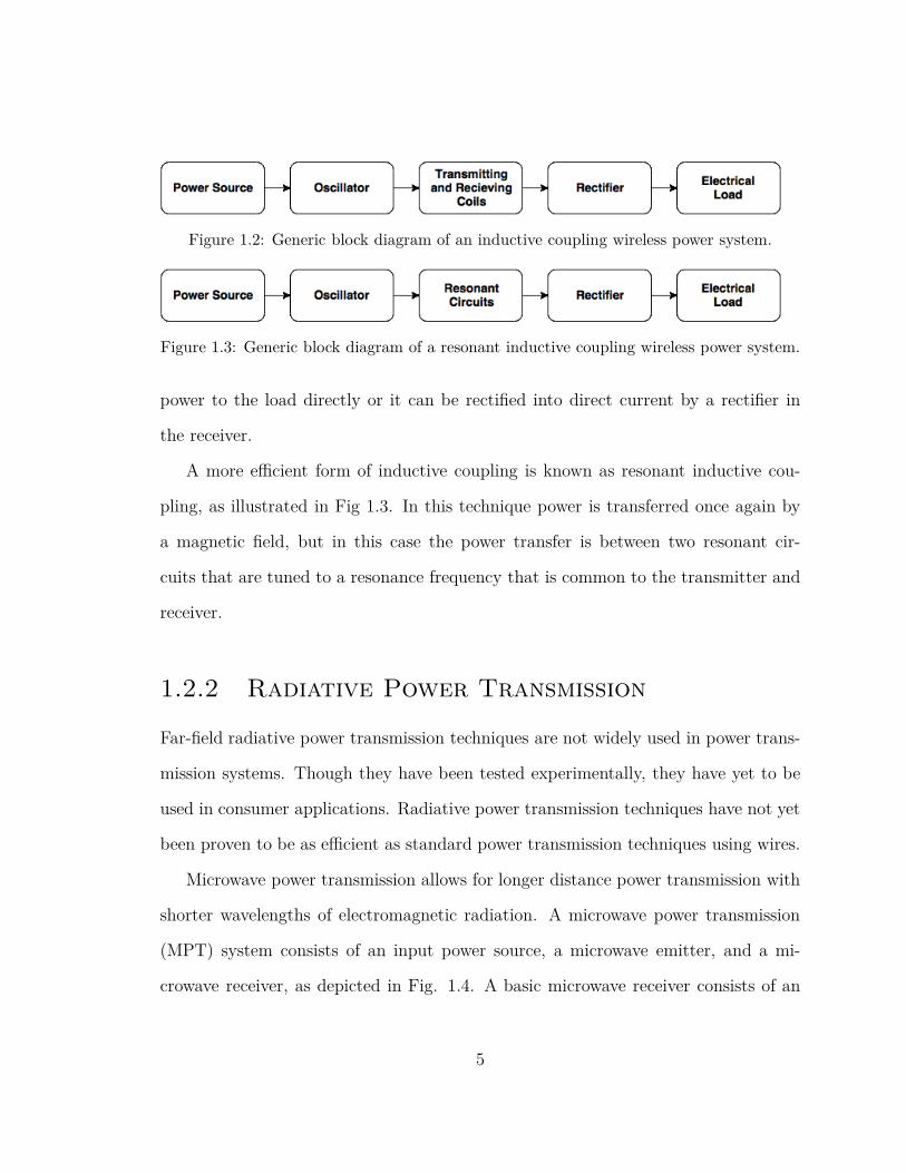
Figure 1.2: Generic block diagram of an inductive coupling wireless power system.
Figure 1.3: Generic block diagram of a resonant inductive coupling wireless power system.
power to the load directly or it can be rectified into direct current by a rectifier in
the receiver.
A more efficient form of inductive coupling is known as resonant inductive cou-
pling, as illustrated in Fig 1.3. In this technique power is transferred once again by
a magnetic field, but in this case the power transfer is between two resonant cir-
cuits that are tuned to a resonance frequency that is common to the transmitter and
receiver.
1.2.2 Radiative Power Transmission
Far-field radiative power transmission techniques are not widely used in power trans-
mission systems. Though they have been tested experimentally, they have yet to be
used in consumer applications. Radiative power transmission techniques have not yet
been proven to be as efficient as standard power transmission techniques using wires.
Microwave power transmission allows for longer distance power transmission with
shorter wavelengths of electromagnetic radiation. A microwave power transmission
(MPT) system consists of an input power source, a microwave emitter, and a mi-
crowave receiver, as depicted in Fig. 1.4. A basic microwave receiver consists of an
5
array of rectifying antennas (a combination of an antenna and a rectifying circuit),
referred to as a rectenna.
The first feasibility study of a MPT system was conducted by William C. Brown
at Raytheon in 1965 [4]. The purpose of this experiment was to power an airborne
microwave supported platform. The platform consisted of a miniature helicopter
equipped with a rectenna array. In this experiment the miniature helicopter was
continuously powered by a microwave beam for ten hours at an altitude of 50 feet,
with an average transmission efficiency that was greater than 90% [4].
A later experiment of note was conducted by the NASA Jet Propulsion Laboratory
in 1975 [5]. This experiment was a "step-up" from Brown’s experiment in regards to
the amount of power being transferred. Specifically, 30 kW of DC output power was
transmitted wirelessly a distance of 1.54 km [5]. The ratio of the total DC power
output to the integrated total available RF power incident on the receiver array was
greater than 80% [5].
1.2.3 Objective of the Project
The primary objective of this research is to investigate a method of propagating a
microwave beam through a spatially inhomogeneous medium more efficiently than
current technologies allow. The method referred to here is the propagation of mi-
crowave power with a so-called Bessel-beam. The unique properties of a Bessel beam
could allow for higher efficiency in MPT. With greater efficiency in MPT, current
aerospace systems and electrical grid infrastructure could be revamped to accommo-
date a global WPT system.
6

Figure 1.4: Microwave power transmission system [5].
1.3 Thesis Overview
This thesis begins with a discussion of the necessary fundamental background from
electromagnetic theory. It includes a brief overview of Maxwell’s equations leading
into the development of electromagnetic wave modes. This pair of orthogonal wave
modes are considered to be either transverse electric or transverse magnetic with
respect to the direction of propagation. Following this development, the description
of a spatially inhomogeneous medium is considered. The inhomogeneous medium
investigated in this thesis is the Earth’s atmosphere. The electromagnetic properties
considered include the electric conductivity σ(ω), the dielectric permittivity ǫ(ω), the
magnetic permeability µ(ω), the refractive index n(ω), and the impedance Z(ω). An
electromagnetic Bessel-beam is then introduced and applied, through a numerical
7
simulation, to microwave beam propagation through the Earth’s atmosphere. The
numerical results presented include an assessment of how well a microwave Bessel-
beam propagates through Earth’s atmosphere and point-to-point in free space.
8

Chapter 2
Fundamental Theory and
Mathematical Preliminaries
2.1 Macroscopic Maxwell’s Equations
The macroscopic Maxwell equations describe the interdependence of the electric field
EEE (r, t) and the magnetic field BBB(r, t) vectors through a set of coupled equations given,
in differential form, by [6]
∇ · DDD(r, t) = ρ(r, t), (2.1a)
∇ · BBB = 0, (2.1b)
∇ × EEE = − ∂
∂tBBB(r, t), (2.1c)
∇ × HHH =∂
∂tDDD(r, t) + JJJ (r, t). (2.1d)
9

in MKS units, where DDD(r, t) is the displacement vector (in coloumb/m2), ρ(r, t) is
the charge density (in coloumb/m3), EEE (r, t) is the electric field intensity vector (in
volt/m), BBB(r, t) is the magnetic induction vector (in tesla), HHH (r, t) is the magnetic
field intensity vector (in ampere/m), and JJJ (r, t) is the current density vector (in
ampere/m2). The two divergence relations are know as Gauss’s law for the electric
and magnetic fields, respectively. The first curl relation is derived from Faraday’s
law and the second from Ampére’s law [3]. This self-consistent set of equations was
first formulated by Maxwell [3] through the inclusion of the displacement current
∂DDD(r, t)/∂t in Ampére’s law.
The charge and current densities appearing in Maxwell’s equations are not in-
dependent quantities. From the physical law of conservation of charge, the charge
density ρ(r, t) and current density JJJ (r, t), which describes the flow of charge, are
related by the equation of continuity
∇ · JJJ (r, t) +∂
∂tρ(r, t) = 0. (2.2)
This equation of continuity is contained in Maxwell’s equations, as can be seen by the
substitution of Eq. (2.1a) into the divergence of Eq. (2.1d). Finally, this set of field
equations is connected to physical measurement through the Lorentz force relation
FFF (r, t) = q(
EEE (r, t) + v(r, t) × BBB(r, t)
)
, (2.3)
where FFF (r, t) is the force acting on a point charge q moving with velocity v(r, t) in
vacuum.
10
2.2 Transverse Electric and Transverse
Magnetic Modes
Consider the propagation of a time-harmonic electromagnetic field in an unbounded
homogeneous, isotropic, conducting region of space. Maxwell’s equations in source-
free regions of space are given by [6]
∇ · EEE = 0, (2.4a)
∇ · HHH = 0, (2.4b)
∇ × EEE = −∂BBB
∂t, (2.4c)
∇ × HHH =∂DDD
∂t+ JJJ , (2.4d)
in MKS units, where
BBB(r, t) =∫ t
−∞
µ(t− t′)HHH (r, t′)dt′ (2.5)
is the magnetic induction field vector,
DDD(r, t) =∫ t
−∞
ǫ(t− t′)EEE (r, t′)dt′ (2.6)
is the electric displacement vector, and
JJJ c(r, t) =∫ t
−∞
σ(t− t′)EEE (r, t′)dt′ (2.7)
11

is the conduction current density. For a strictly monochromatic field of angular
frequency ω, one sets
EEE (r, t) = ℜ
E(r)eiωt
, (2.8a)
HHH (r, t) = ℜ
H(r)eiωt
, (2.8b)
where E and H are the complex phasor representations of the electric and magnetic
field vectors. With this substitution, Maxwell’s equations (2.4) assume their time-
harmonic (or phasor) form
∇ · E = 0, (2.9a)
∇ · H = 0, (2.9b)
∇ × E = −iωµ(ω)H, (2.9c)
∇ × H = iωǫc(ω)E, (2.9d)
after application of the convolution theorem, where
µ(ω) =∫
∞
−∞
µ(t)eiωtdt, (2.10a)
ǫ(ω) =∫
∞
−∞
ǫ(t)eiωtdt, (2.10b)
σ(ω) =∫
∞
−∞
σ(t)eiωtdt, (2.10c)
12

are the magnetic permeability, dielectric permittivity and electric conductivity, re-
spectfully. The complex permittivity appearing in Eq. (2.9d) is defined as
ǫc(ω) = ǫ(ω) + iσ(ω)
ω(2.11)
and will be touched upon again in Chapter 3. Upon taking the curl of Eq. (2.9c) and
using Eqs. (2.9a) and (2.9d), one obtains
∇ × (∇ × E)︸ ︷︷ ︸
∇(∇ · E)︸ ︷︷ ︸
0
−∇2E
= −iµω∇ × H︸ ︷︷ ︸
iǫcωE
∴ ∇2E + µǫcω2E = 0. (2.12)
Similarly, upon taking the curl of Eq. (2.9d) and using (2.9b) and (2.9c), there results
∇ × (∇ × H)︸ ︷︷ ︸
∇(∇ · H)︸ ︷︷ ︸
0
−∇2H
= iωǫc ∇ × E︸ ︷︷ ︸
iµωH
∴ ∇2H + µǫω2H = 0. (2.13)
The wavenumber of the monochromatic field is given by
k(ω) = ω[
µǫ(ω)
]1/2
=ω
cn(ω)
(2.14)
13

where n(ω) is the refractive index of the medium defined as
n(ω) =
[
µǫ(ω)
µ0ǫ0
]1/2
, (2.15)
where c = 1/√µ0ǫ0 is the speed of light in a vacuum. With these identifications,
Eqs. (2.13) and (2.14) become
∇2E + k2(ω)E = 0 (2.16)
∇2H + k2(ω)H = 0. (2.17)
These equations are known as the Helmholtz equations [3].
2.2.1 TE and TM Modes in Rectangular
Coordinates
The phasor electric and magnetic field vectors in rectangular coordinates for a time-
harmonic electromagnetic wave propagating in the z-direction may then be repre-
sented in component form as
E = 1xEx + 1yEy + 1zEz, (2.18a)
H = 1xHx + 1yHy + 1zHz. (2.18b)
14

With this substitution the field equations (2.9) become
∂Ex
∂x+
∂Ey
∂y+∂Ez
∂z= 0 (2.19a)
∂Hx
∂x+∂Hy
∂y+∂Hz
∂z= 0 (2.19b)
∂Ez
∂y− ∂Ey
∂z= −iµωHx (2.19c)
∂Ex
∂z− ∂Ez
∂x= −iµωHy (2.19d)
∂Ey
∂x−∂Ex
∂y= −iµωHz (2.19e)
∂Hz
∂y− ∂Hy
∂z= iǫωEx (2.19f)
∂Hx
∂z− ∂Hz
∂x= iǫωEy (2.19g)
∂Hy
∂x−
∂Hx
∂y= iǫωEz (2.19h)
In order to simplify the analysis, attention is now turned to "two dimensional" di-
electric regions in which there is no spatial variation of the field vectors along the
y-direction, so that ∂/∂y = 0 for each component of each field vector. The above set
of equations then separates into two distinct groups as follows:
∂Hx
∂x+∂Hz
∂z= 0
∂Ey
∂z= iµωHx
∂Ey
∂x= −iµωHz
∂Hx
∂z− ∂Hz
∂x= iǫωEy
E = 1yEy
H = 1xHx + 1zHz
(2.20)
15

and∂Ex
∂x+∂Ez
∂z= 0
∂Ex
∂z− ∂Ez
∂x= −iµωHy
∂Hy
∂z= −iǫωEx
∂Hy
∂x= iǫωEz
E = 1xEx + 1zEz
H = 1yHy
(2.21)
Upon differentiating the second relation in Eq. (2.20) with respect to z and the third
with respect to x and adding the two results yields, after use of the the first and
fourth relations in Eq. (2.20),
∂2Ey
∂x2+∂2Ey
∂z2+ω2
c2n2Ey = 0
Hx = − i
µω
∂Ey
∂z
Hz =i
µω
∂Ey
∂x
TE Modes (2.22)
where
ETE = 1yEy,
HTE = 1xHx + 1zHz.
(2.23)
These are called TE modes because the electric field vector does not have a component
along the propagation direction (the z-direction).
In a similar manner, differentiation of the third relation in Eq. (2.21) with respect to
z and the fourth with respect to x and adding the two results together yields, after
16

use of the first and second relations in Eq. (2.21),
∂2Hy
∂x2+∂2Hy
∂z2+ω2
c2n2Hy = 0
Ex =i
ǫω
∂Hy
∂z
Ez = − i
ǫω
∂Hy
∂x
TM Modes (2.24)
where
ETM = 1xEx + 1zEz
HTM = 1yHy.
(2.25)
These are called TM modes because the magnetic field vector does not have a z-
component. Notice that ETE · ETM = HTE · HTM = 0 so that they are mutually
orthogonal fields.
2.2.2 TE and TM Modes in Cylindrical
Coordinates
In cylindrical coordinates (ρ, φ, z) the field vectors are expressed in the form
E = 1ρEρ + 1φEφ + 1zEz (2.26a)
H = 1ρHρ + 1φHφ + 1zHz (2.26b)
where ρ =√x2 + y2 is the radial distance perpendicular to and from the z-axis and
φ = tan−1(y/x) is the azimuthal angle measured from the positive x-axis. With this
17
substitution the field equations (2.9) take on the component form
1
ρ
∂(ρEρ)
∂ρ+
1
ρ
∂Eφ
∂φ+∂Ez
∂z= 0 (2.27a)
1
ρ
∂(ρHρ)
∂ρ+
1
ρ
∂Hφ
∂φ+∂Hz
∂z= 0 (2.27b)
1
ρ
∂Ez
∂φ− ∂Eφ
∂z= −iµωHρ (2.27c)
∂Eρ
∂z− ∂Ez
∂ρ= −iµωHφ (2.27d)
1
ρ
∂(ρEφ)
∂ρ−
1
ρ
∂Eρ
∂φ= −iµωHz (2.27e)
1
ρ
∂Hz
∂φ− ∂Hφ
∂z= iǫωEρ (2.27f)
∂Hρ
∂z− ∂Hz
∂ρ= iǫωEφ (2.27g)
1
ρ
∂(ρHφ)
∂ρ−
1
ρ
∂Hρ
∂φ= iǫωEz (2.27h)
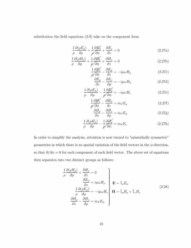
In order to simplify the analysis, attention is now turned to "azimuthally symmetric"
geometries in which there is no spatial variation of the field vectors in the φ-direction,
so that ∂/∂φ = 0 for each component of each field vector. The above set of equations
then separates into two distinct groups as follows:
1
ρ
∂(ρHρ)
∂ρ+∂Hz
∂z= 0
∂Eφ
∂z= iµωHρ
1
ρ
∂(ρEφ)
∂ρ= −iµωHz
∂Hρ
∂z− ∂Hz
∂ρ= iǫωEφ
E = 1φEφ
H = 1ρHρ + 1zHz
(2.28)
18
1
ρ
∂(ρEρ)
∂ρ+∂Ez
∂z= 0
−∂Hφ
∂z= iǫωEρ
1
ρ
∂(ρHφ)
∂ρ= −iǫωEz
∂Eρ
∂z− ∂Ez
∂ρ= iµωEφ
E = 1ρEρ + 1zEz
H = 1φHφ
(2.29)
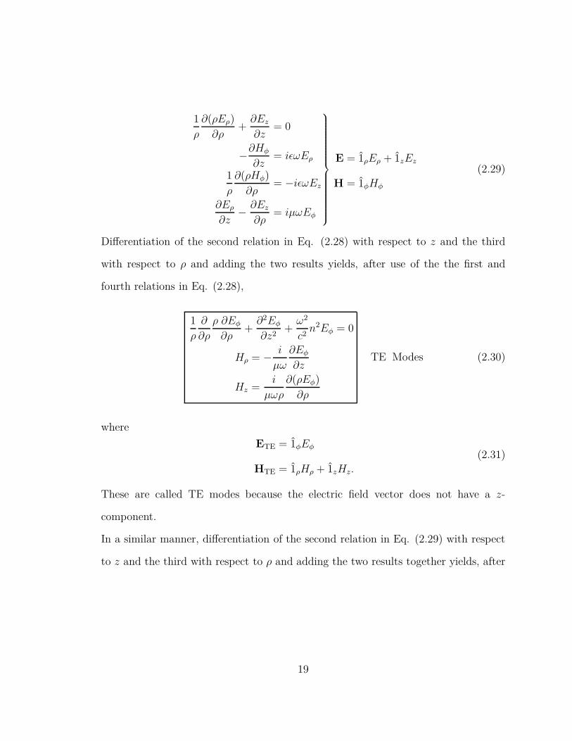
Differentiation of the second relation in Eq. (2.28) with respect to z and the third
with respect to ρ and adding the two results yields, after use of the the first and
fourth relations in Eq. (2.28),
1
ρ
∂
∂ρ
ρ ∂Eφ
∂ρ+∂2Eφ
∂z2+ω2
c2n2Eφ = 0
Hρ = − i
µω
∂Eφ
∂z
Hz =i
µωρ
∂(ρEφ)
∂ρ
TE Modes (2.30)
where
ETE = 1φEφ
HTE = 1ρHρ + 1zHz.
(2.31)
These are called TE modes because the electric field vector does not have a z-
component.
In a similar manner, differentiation of the second relation in Eq. (2.29) with respect
to z and the third with respect to ρ and adding the two results together yields, after
19
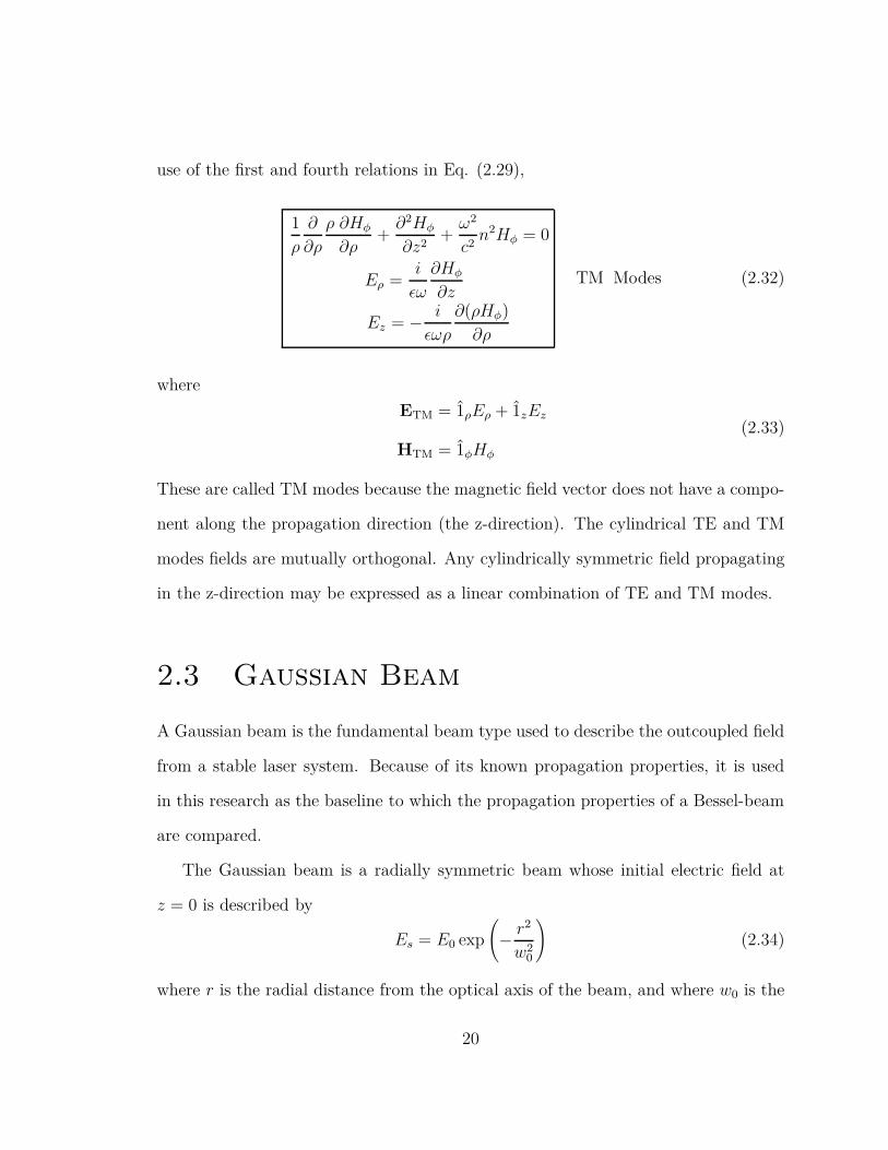
use of the first and fourth relations in Eq. (2.29),
1
ρ
∂
∂ρ
ρ ∂Hφ
∂ρ+∂2Hφ
∂z2+ω2
c2n2Hφ = 0
Eρ =i
ǫω
∂Hφ
∂z
Ez = − i
ǫωρ
∂(ρHφ)
∂ρ
TM Modes (2.32)
where
ETM = 1ρEρ + 1zEz
HTM = 1φHφ
(2.33)
These are called TM modes because the magnetic field vector does not have a compo-
nent along the propagation direction (the z-direction). The cylindrical TE and TM
modes fields are mutually orthogonal. Any cylindrically symmetric field propagating
in the z-direction may be expressed as a linear combination of TE and TM modes.
2.3 Gaussian Beam
A Gaussian beam is the fundamental beam type used to describe the outcoupled field
from a stable laser system. Because of its known propagation properties, it is used
in this research as the baseline to which the propagation properties of a Bessel-beam
are compared.
The Gaussian beam is a radially symmetric beam whose initial electric field at
z = 0 is described by
Es = E0 exp
(
− r2
w20
)
(2.34)
where r is the radial distance from the optical axis of the beam, and where w0 is the
20
0 0.5 1 1.5 2 2.5 3 3.5 4
Normalized Radius (r/w0)
0
0.1
0.2
0.3
0.4
0.5
0.6
0.7
0.8
0.9
1E
s/E0
Gaussian Beam Signal Intensity
e-1 ⇓
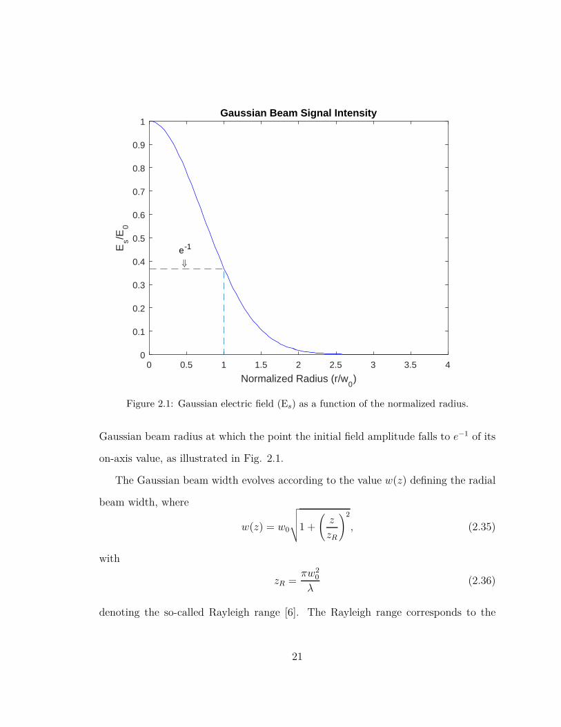
Figure 2.1: Gaussian electric field (Es) as a function of the normalized radius.
Gaussian beam radius at which the point the initial field amplitude falls to e−1 of its
on-axis value, as illustrated in Fig. 2.1.
The Gaussian beam width evolves according to the value w(z) defining the radial
beam width, where
w(z) = w0
√√√√1 +
(
z
zR
)2
, (2.35)
with
zR =πw2
0
λ(2.36)
denoting the so-called Rayleigh range [6]. The Rayleigh range corresponds to the
21

Figure 2.2: Gaussian beam width ω(z) as a function of the distance z along the beam.
distance zR from the beam waist at z = 0 where the beam width w(z) has increased
to√
2 times larger than its value w(0) = w0 at z = 0. At this point the on-axis
intensity has decreased to half of its peak value at z = 0.
As z becomes much greater than the Rayleigh range, the beam half-width w(z)
increases linearly with z. The angle describing the divergence of the beam is given
by
θ =λ
πw0, (2.37)
as illustrated in Fig. 2.2. The full angular spread of the beam far from the beam waist
is then given by Θ = 2θ. Notice that the beam divergence is inversely proportional
to the spot size for a given wavelength, so that a decrease in the beam waist size w0
results in an increase of the beam divergence Θ = 2θ accompanied by a decrease in
the Rayleigh range zR.
22

Chapter 3
Electromagnetic Characteristics
of the Earth’s Atmosphere
3.1 Spatially Inhomogeneous Media
Electromagnetic wave propagation is directly effected by the properties of the medium
it is traveling through. The electromagnetic properties characterizing any given
medium include the electric conductivity σ(ω) (in Siemens/meter or mhos/meter
/m), the dielectric permittivity ǫ(ω) (in Farads/meter), and the magnetic perme-
ability µ(ω) (in Henries/meter). The refractive index n(ω) =√
ǫ(ω)µ(ω)/ǫ0µ0, which
is dimensionless, and impedance Z(ω) =√
µ(ω)/ǫ(ω) (in ohms (Ω)), are derived from
these fundamental material parameters.
23

3.1.1 Earth’s Atmosphere
With regards to its electromagnetic characteristics, the Earth’s atmosphere is par-
titioned into three distinct vertical regions: a non-ionized region, an ionized region,
and free-space. The non-ionized region extends from sea level up to approximately
90km above sea level. In this region, the electromagnetic characteristics are primar-
ily affected by temperature, water vapor pressure and atmospheric pressure. The
ionized region extends from 90km up to 1,000km above sea level. In this region
the electromagnetic characteristics are primarily affected by the electron density, the
electron and ion temperatures, and the ionic composition. The uppermost portion
of the atmosphere is referred to as free-space, extending from 1,000km to 35,700km
(geosynchronous orbit) above sea level. The properties in this region are defined to
be those in a vacuum. The region above free-space is known as interplanetary space.
3.1.2 Mars’ Atmosphere
The Martian atmosphere consists of a four regions, all of which are much less dense
than the Earth’s Atmosphere. The layers of Mars’s atmosphere are known as the ex-
osphere, thermosphere, middle atmosphere, and lower atmosphere [7]. The exosphere
starts at about 200km above the surface of Mars and extends upwards to where the
atmosphere merges with the vacuum of space. There is no distinct region where the
atmosphere ends. The thermosphere is the region below the exosphere with very
high temperatures caused by heating from the sun. In this region atmospheric gases
start to separate from each other rather than forming the even mixture that exists
at lower atmospheric layers. The middle atmosphere is the region in which Mars’ jet
24
stream flows. The lower atmosphere is a relatively warm region affected by heat from
airborne dust and the ground.
With regards to the electromagnetic properties of Mars’s atmosphere, they can
be deemed negligible. The Martian atmosphere is approximately 0.6% as dense as
Earth’s atmosphere [7]. Knowing this it can be assumed when running electromag-
netic simulations of Mars’s atmosphere that it can have the same properties as a
vacuum.
3.2 Electric Conductivity
Electric conductivity σ(ω) is a measure of a materials ability to accommodate the
transport of electric charge. This material parameter is measured in either Siemens
per meter (S/m) or mhos per meter (/m).
In the case of the Earth’s atmosphere, the electric conductivity possesses three
components, each dependent upon altitude. The parallel or field-aligned conductivity
σ0(z) describes the conductivity in the direction parallel to the Earth’s magnetic field.
The field-aligned conductivity is by far the largest of the three Earth’s conductivity
components. The Pedersen conductivity σ1(z) is in the direction vertical to the
Earth’s magnetic field and parallel to the electric field originating at the magnetic
poles. Finally, the Hall conductivity σ2(z) is in the direction vertical to both of these
magnetic and electric fields. A comparison of the field-aligned conductivity σ0(z) and
Pedersen conductivity σ1(z) as a function of altitude z above sea level is shown in
Fig. 3.1. As can be seen, σ1(z) is at least 12 orders of magnitude down from σ0(z)
throughout the Earth’s atmosphere.
25

100 200 300 400 500 600 700 800 900 1000
Altitude z (km)
10-20
10-15
10-10
10-5
100
105
Con
duct
ivity
(S
/m)
Conductivity vs. Altitude
σ0
σ1
Figure 3.1: Field-aligned and Pedersen conductivity measured in S/m corresponding to spe-cific altitudes in the first 1,000km of the Earth’s atmosphere. Notice that the conductivityvanishes in the non-ionized region and in free space at altitudes higher than 1,000km. Dataprovided by Dao et al [8].
26
3.3 Dielectric Permittivity
The dielectric permittivity is a measure of the ability of a medium to capacitively
store electric field energy and is accordingly measured in Farads per meter (F/m).
The permittivity of free space is given by ǫ0 = 8.845 × 10⁻¹² F/m. The permittivity
ǫ(z, ω) in a spatially inhomogeneous medium such as the Earth’s atmosphere can be
represented as
ǫ(z, ω) = ǫ0ǫr(z, ω) (3.1)
where ǫr(z, ω) = ǫ(z, ω)/ǫ0 is the relative permittivity of the medium [6]. The de-
pendence of ǫ on the frequency of the electromagnetic field is known as temporal
dispersion and its dependence on the distance z above sea-level is referred to as spa-
tial inhomogeneity.
3.3.1 Complex Permittivity
The complex permittivity combines to dielectric permittivity ǫ(z, ω) and electric con-
ductivity into a single quantity that characterizes the frequency dependent electrical
properties of the material. This was defined in Eq. (2.11) in connection with the
phasor form of Ampére’s law as
ǫc(ω) = ǫ(ω) + iσ(ω)
ω. (3.2)
If the static conductivity σ0 = σ(0) is nonzero, then the complex permittivity has a
simple pole at the origin ω = 0. Furthermore this equation can be broken down into
27

real and imaginary parts as
ǫc(ω) =(
ǫr(ω) − σi(ω)
ω
)
+ i(
ǫi(ω) +σr(ω)
ω
)
, (3.3)
where ǫr(ω) = ℜǫ(ω) is the real part of the permittivity, which is related to the
reactively stored energy within the medium, and ǫi(ω) = ℑǫ(ω) is the imaginary
part of the permittivity, which is related to the dissipation of energy within the
medium [6]. Since the conductivity through the Earth’s atmosphere is purely real the
complex dielectric permittivity can be calculated, in this case, using
ǫc(ω) = ǫr(ω) + i(
ǫi(ω) +σr(ω)
ω
)
. (3.4)
Using the previously shown values for the field-aligned conductivity and values for
the permittivity from Dao et al. [8] the relative complex permittivity was calculated.
The results are shown with respect to the altitude z in Fig. 3.2. It can be seen in
Fig. 3.2 that because the conductivity is, within the approximation of the present
analysis, purely real, the conductivity only has an effect on the imaginary part of the
complex permittivity, as seen in Fig. 3.2 where the imaginary part and magnitude of
the relative complex permittivity are overlapping.
28

0 100 200 300 400 500 600 700 800 900 1000
Altitude z (km)
10-1
100
101
102
103
104
Rel
ativ
e C
ompl
ex P
erm
ittiv
ity
Relative Complex Permittivity vs. Altitude
ℜ(ǫc)/ǫ
0
ℑ(ǫc)/ǫ
0
|ǫc|/ǫ
0
Figure 3.2: Complex permittivity (in F/m) corresponding to specific altitudes in the first1,000km of the Earth’s atmosphere. Notice that the magnitude and imaginary part of therelative complex permittivity are overlapping in the ionized region. Beyond the ionizedregion, the permittivity is that of free space. Data calculated using data published by Daoet al. [8].
29
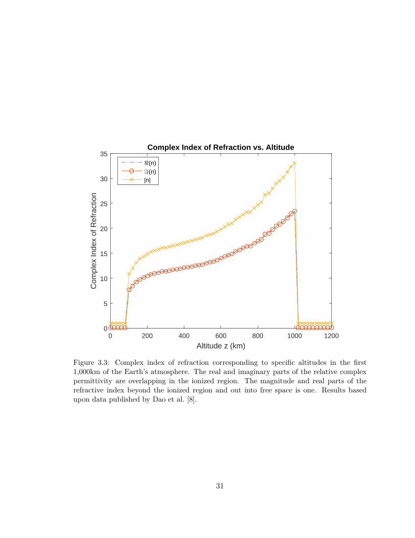
3.4 Refractive Index
The refractive index is defined in terms of the complex dielectric permittivity and
relative magnetic permeability as
n(z, ω) =
√
µrǫc(z, ω)
ǫ0(3.5)
where µr is the relative magnetic permeability [6]. In the case of the Earth’s atmo-
sphere, µr∼= 1. The calculated index of refraction corresponding to altitude is shown
in Fig 3.3. Notice that the real and imaginary parts of the index of refraction are
overlapping because the conductivity is purely real, having an equal effect on the real
and imaginary parts.
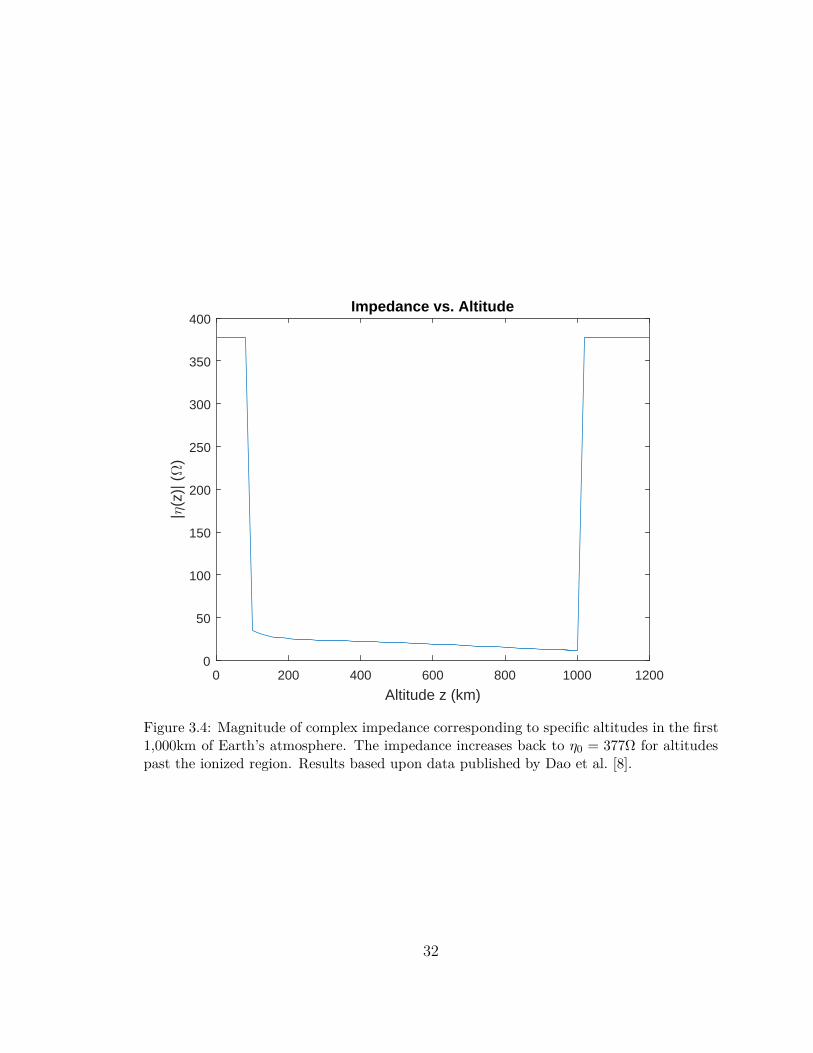
3.5 Impedance
The impedance η(z, ω) of each layer of the atmosphere is related to its permittivity
by the relation
η(z, ω) =
√
µr
ǫc(ω)/ǫ0η0 (3.6)
where η0 =√
µ0/ǫ0 = 377Ω is the impedance of free space [9]. A plot of the com-
plex intrinsic impedance of the Earth’s atmosphere versus altitude z is illustrated in
Fig. 3.4.
30
0 200 400 600 800 1000 1200
Altitude z (km)
0
5
10
15
20
25
30
35
Com
plex
Inde
x of
Ref
ract
ion
Complex Index of Refraction vs. Altitude
ℜ(n)ℑ(n)|n|
Figure 3.3: Complex index of refraction corresponding to specific altitudes in the first1,000km of the Earth’s atmosphere. The real and imaginary parts of the relative complexpermittivity are overlapping in the ionized region. The magnitude and real parts of therefractive index beyond the ionized region and out into free space is one. Results basedupon data published by Dao et al. [8].
31
0 200 400 600 800 1000 1200
Altitude z (km)
0
50
100
150
200
250
300
350
400
|η(z
)| (Ω
)
Impedance vs. Altitude
Figure 3.4: Magnitude of complex impedance corresponding to specific altitudes in the first1,000km of Earth’s atmosphere. The impedance increases back to η0 = 377Ω for altitudespast the ionized region. Results based upon data published by Dao et al. [8].
32

3.6 Reflection and Transmission
Coefficients
The reflection and transmission coefficients are determined by the impedance change
from one layer to another. At each interface there is a corresponding reflection and
transmission coefficient. The reflection coefficient Γ describes what fraction of the
electric field amplitude is reflected back. The transmission coefficient τ describes
what fraction of the electric field amplitude is transmitted in the forward direction.
With regard to the layered atmosphere model considered here,
Γij =ηj − ηi
ηj + ηi
(3.7)
and
τij =2ηj
ηj + ηi(3.8)
where ηi is the impedance of the medium where the incident wave field resides and ηj
is the impedance of the medium where the transmitted wave field resides [9]. A plot
of the reflection and transmission coefficients is shown in Fig. 3.5 as a function of the
interference number j. The vertical thickness of each layer is given by ∆z = 20km so
that the height of each layer above the Earth’s surface is given by zj = j∆z.
33

0 5 10 15 20 25 30 35 40 45 50
Interface Number
0
0.2
0.4
0.6
0.8
1
1.2
Ref
lect
ion
and
Tra
nsm
issi
on C
oeffi
cien
ts
Reflection and Transmission Coefficients at Interfaces
|Γ||τ|
Figure 3.5: Reflection and Transmission coefficients corresponding to impedance interfacesin the first 1,000km of Earth’s atmosphere. The large dip at interface 5 is due to a largeimpedance change from the non-ionized region to the ionized region of the Earth’s atmo-sphere. At all other interfaces, practically all of the field is transmitted at each layer.Results based upon data published by Dao et al. [8].
34
Chapter 4
Electromagnetic Bessel Beam
4.1 Scalar Wave Formulation
The goal in this section is to deduce the form of a cylindrically symmetric plane wave
that propagates in a vacuum, known as a Bessel beam. This is done based upon the
derivation given by K. T. McDonald [10]. A scalar, azimuthally symmetric wave of
frequency ω that propagates in the z-direction may be written as
ψ(r, t) = f(ρ)ei(kzz−ωt), (4.1)
where ρ =√x2 + y2. The problem is then to deduce the form of the radial function
f(ρ) together with any relevant condition on the wave number kz, and then to relate
Eq. (4.1) to a complete set of Maxwell’s equations.
The first step is to determine the precise form of the radial function f(ρ) that
35

satisfies the scalar wave equation
∇2ψ =1
c2
∂2ψ
∂t2. (4.2)
Substitution of Eq. (4.1) into this wave equation then yields
d2f
dρ2+
1
ρ
df
dρ+ (k2 − k2
z) = 0. (4.3)
This is precisely the differential equation defining Bessel functions of order 0, so that
f(ρ) = J0(kρρ), (4.4)
where
k2ρ + k2
z = k2. (4.5)
The form of (4.5) suggests that we introduce a real parameter α such that
kρ = k sinα, (4.6a)
kz = k cosα. (4.6b)
The desired cylindrical plane wave then assumes the form
ψ(r, t) = J0(kρ sinα)ei(kz cos α−ωt), (4.7)
which is referred to as a Bessel beam [10].
36

4.2 Electromagnetic Formulation
The next step in the analysis is to determine each component of the electric and
magnetic fields of a Bessel beam through Maxwell’s equations. This is accomplished
through the determination of the vector potential A from the scalar wave function
ψ(r, t) given in Eq. (4.7). This analysis is performed in the Lorenz gauge where the
scalar potential Φ is related to the vector potential A through the Lorenz condition
∇ · A + ǫ0µ0∂Φ
∂t= 0. (4.8)
The vector potential can therefore have a nonzero divergence. The electric and mag-
netic fields are then determined by the vector and scalar potentials as
E = −∇Φ − ∂A
∂t, (4.9)
and
B = ∇ × A. (4.10)
The scalar potential is then determined from the vector potential using the Lorenz
condition and the electric field then follows from Eq. (4.9). For a wave-field with
constant frequency ω and time dependence of the form e−iωt, so that ∂Φ/∂t = −iωΦ.
The Lorenz condition then yields
Φ = −i ck
∇ · A, (4.11)
37
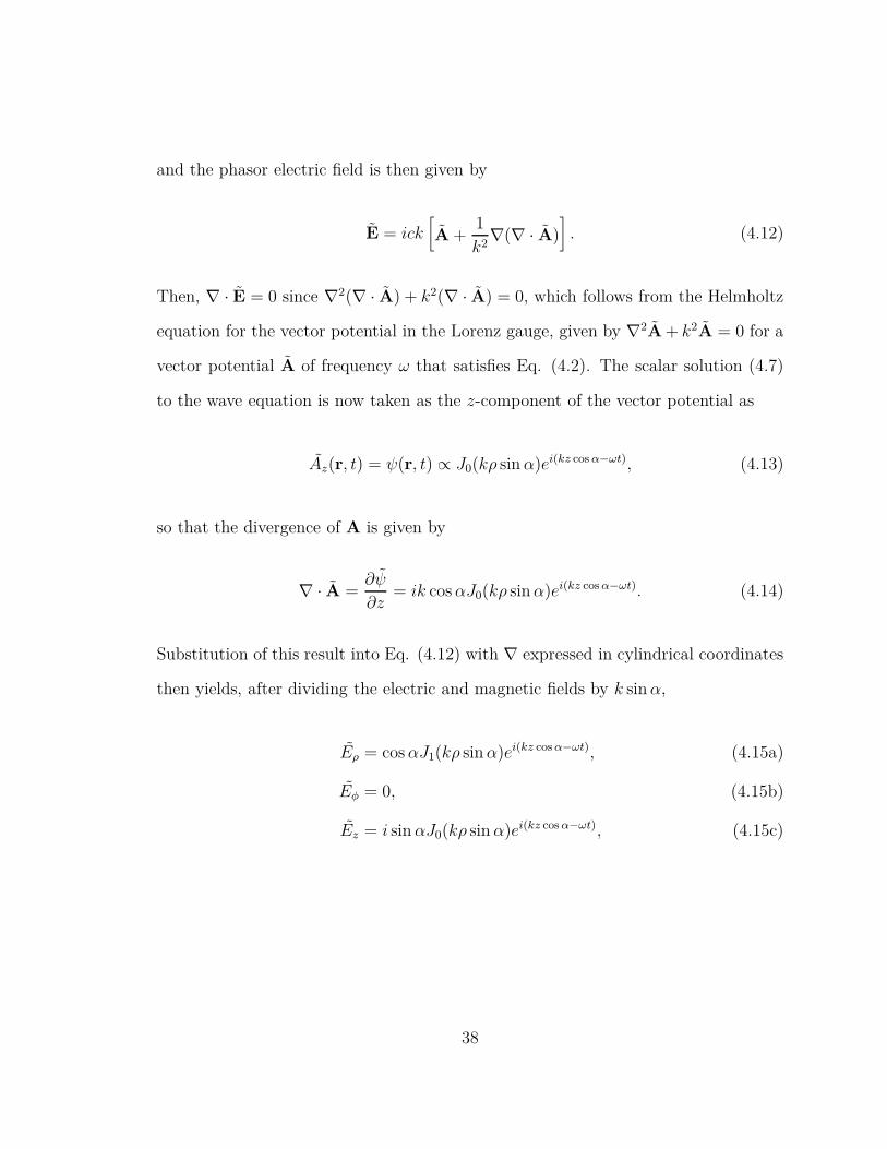
and the phasor electric field is then given by
E = ick[
A +1
k2∇(∇ · A)
]
. (4.12)
Then, ∇ · E = 0 since ∇2(∇ · A) + k2(∇ · A) = 0, which follows from the Helmholtz
equation for the vector potential in the Lorenz gauge, given by ∇2A + k2A = 0 for a
vector potential A of frequency ω that satisfies Eq. (4.2). The scalar solution (4.7)
to the wave equation is now taken as the z-component of the vector potential as
Az(r, t) = ψ(r, t) ∝ J0(kρ sinα)ei(kz cos α−ωt), (4.13)
so that the divergence of A is given by
∇ · A =∂ψ
∂z= ik cosαJ0(kρ sinα)ei(kz cos α−ωt). (4.14)
Substitution of this result into Eq. (4.12) with ∇ expressed in cylindrical coordinates
then yields, after dividing the electric and magnetic fields by k sinα,
Eρ = cosαJ1(kρ sinα)ei(kz cos α−ωt), (4.15a)
Eφ = 0, (4.15b)
Ez = i sinαJ0(kρ sinα)ei(kz cos α−ωt), (4.15c)
38
and
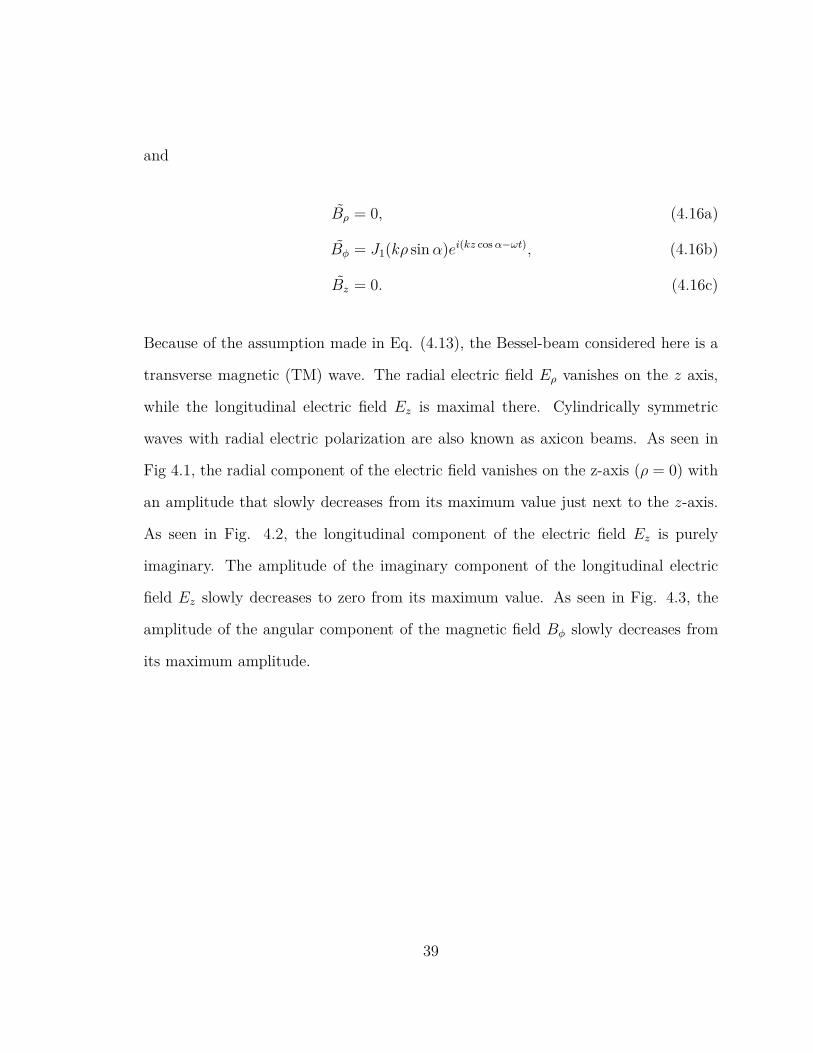
Bρ = 0, (4.16a)
Bφ = J1(kρ sinα)ei(kz cos α−ωt), (4.16b)
Bz = 0. (4.16c)
Because of the assumption made in Eq. (4.13), the Bessel-beam considered here is a
transverse magnetic (TM) wave. The radial electric field Eρ vanishes on the z axis,
while the longitudinal electric field Ez is maximal there. Cylindrically symmetric
waves with radial electric polarization are also known as axicon beams. As seen in
Fig 4.1, the radial component of the electric field vanishes on the z-axis (ρ = 0) with
an amplitude that slowly decreases from its maximum value just next to the z-axis.
As seen in Fig. 4.2, the longitudinal component of the electric field Ez is purely
imaginary. The amplitude of the imaginary component of the longitudinal electric
field Ez slowly decreases to zero from its maximum value. As seen in Fig. 4.3, the
amplitude of the angular component of the magnetic field Bφ slowly decreases from
its maximum amplitude.
39

0 5 10 15 20 25
ρ (meters)
-0.4
-0.3
-0.2
-0.1
0
0.1
0.2
0.3
0.4
0.5
0.6
Am
plitu
de o
f Eρ
Radial Electric Field at t=0
Figure 4.1: Radial electric field (Eρ) as a function of the radial distance ρ from the z-axis.
40

0 5 10 15 20 25
ρ (meters)
-0.04
-0.02
0
0.02
0.04
0.06
0.08
0.1
Am
plitu
de o
f Ez
Longitudinal Electric Field at t=0
ℜ(Ez)
ℑ(Ez)
Figure 4.2: Longitudinal electric field (Ez) as a function of the radial distance ρ from thez-axis.
41
0 5 10 15 20 25
ρ (meters)
-0.4
-0.3
-0.2
-0.1
0
0.1
0.2
0.3
0.4
0.5
0.6
Am
plitu
de o
f Bφ
Angular Magnetic Field at t=0
Figure 4.3: Angular magnetic field component (Bφ) as a function of the radial distance ρ
from the z-axis.
42
0 5 10 15 20 25
ρ (meters)
-0.4
-0.3
-0.2
-0.1
0
0.1
0.2
0.3
0.4
0.5
0.6
Am
plitu
de o
f E a
nd B
fiel
ds
E and B field comparison at t=0
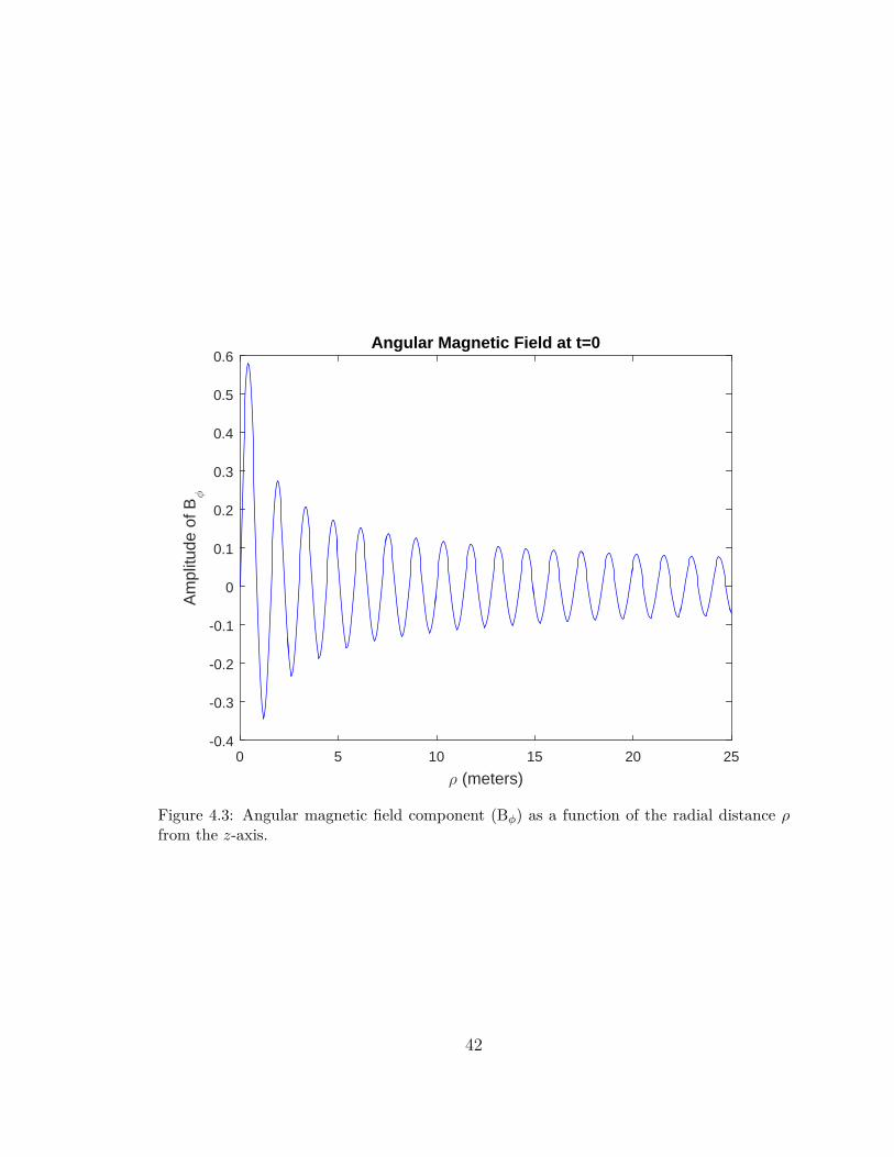
Eρ
ℑ(Ez)
Bφ
Figure 4.4: Comparison of the amplitudes of the radial electric field, imaginary part of thelongitudinal electric field and the angular magnetic field as a function of the radius. Theradial electric field and the angular magnetic field are overlapping.
43
0 5 10 15 20 25
ρ (meters)
-0.4
-0.2
0
0.2
0.4
0.6
0.8
1
Sig
nal
Scalar and Radial Electromagnetic Waves
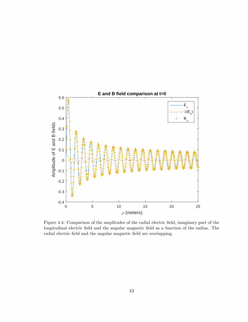
Eρ
ψ(r,t)
Figure 4.5: Comparison of the scalar wave equation and the radial electromagnetic fields.
44

4.3 Bessel-Beam Construction
The physical realization of a Bessel-beam has been achieved using a variety of ex-
perimental methods. Some of these methods produce what is considered a pseudo-
Bessel-beam [1] and others a true Bessel-beam [1]. In the present research only the
true mathematical model of a Bessel beam was considered and simulated.
The first Bessel-beam launcher reported in open literature consists of a diffracting
ring placed at the focal distance of a convergent lens and illuminated by a plane wave
[1], as shown in Fig. 4.6. Light diffracts as it passes through the ring. After passing
through the lens, the diffracted rays interfere with each other and thereby form form
a pseudo-Bessel-beam. This launcher suffers from very low efficiency because most of
the beam power is blocked by the diaphragm. This problem can be overcome using
an axicon lens, shown in Fig. 4.7, which is more commonly used today. An axicon
lens has a flat entrance surface and an output volume shaped into a cone. When a
plane wave is incident upon the conic surface, the light refracts into a converging conic
beam and thereby forms a pseudo-Bessel-beam over the region of overlap illustrated
in the figure.
45
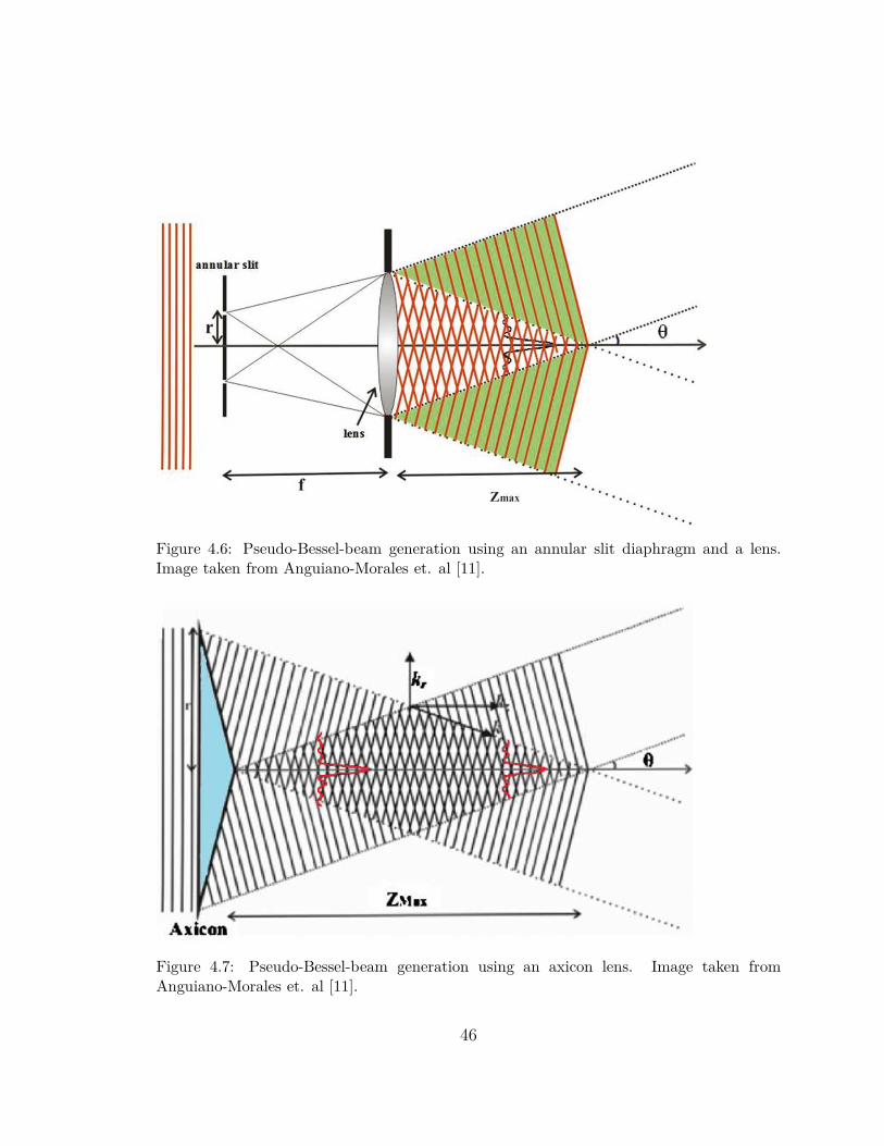
Figure 4.6: Pseudo-Bessel-beam generation using an annular slit diaphragm and a lens.Image taken from Anguiano-Morales et. al [11].
Figure 4.7: Pseudo-Bessel-beam generation using an axicon lens. Image taken fromAnguiano-Morales et. al [11].
46
Chapter 5
Microwave Bessel-Beam
Propagation
5.1 Numerical Simulation of Bessel-Beam
In order to investigate the propagation of a microwave Bessel-beam, one must first
model the plane wave spectrum representation of the electromagnetic beam field in
MATLAB. Creating the plane wave spectrum representation of the electromagnetic
beam field of a Bessel-beam in cylindrical coordinates requires the implementation of
several mathematical procedures related to the proper numerical implementation of
the Quasi-fast Hankel transform (QFHT) and its inverse Quasi-fast Hankel transform
(IQFHT) described in Appendix A. These include the application of a so-called guard
band to minimize numerical aliasing errors.
The numerical implementation of a guard band is vital when creating the plane
wave spectrum representation of an electromagnetic beam field. The purpose of the
guard band is to pad zeros at the end of a signal out a certain distance in order
47

to minimize the effects of numerical aliasing. This distance measured is relative to
the radius of the source aperture as well as the electromagnetic characteristics of
the region into which the signal is propagated, taking into account the transverse
spreading of the electromagnetic beam field as it propagates.
The QFHT algorithm is used here instead of the rectangular coordinate FFT
in order to take advantage of the cylindrical symmetry of the Bessel-beam. The
QFHT algorithm transforms a radially dependent field into an angular spectrum
representation of plane waves. Each spectral component can then be propagated
the distance z through multiplication by an exponential phase factor. The resulting
spectrum is then transformed back into the radial space domain using the IQFHT.
This propagation algorithm is described in Appendix B.
5.2 Transmission in Free Space
The primary effect that effects propagation through vacuum is diffraction and this is
most conveniently described through the Fresnel number
N =a2
λ∆z, (5.1)
where a is the beam radius, λ is the wavelength, and ∆z is the propagation distance.
The simulations done in this research correspond to an aperture with a 25 meter
radius and 1 degree structure angle corresponding to α in Eqs. (4.15 - 4.16). The
following figures show the evolution of the radial electric field strength as the Bessel-
beam propagates away from the initial plane through a vacuum.
48

02000
0.2
0.4
1500 50
Inte
nsity 0.6
Bessel Beam Propagation
Propagation Distance (meters)
1000
0.8
Radius (meters)
1
0500
0 -50
0.1
0.2
0.3
0.4
0.5
0.6
0.7
0.8
0.9
1
Figure 5.1: Surface plot depicts the relative intensity of the radial electric field (Eρ) of aBessel-beam as a function of the radius as the beam propagates over 2,000 meters from thesource aperture in free-space.
49

Bessel Beam Intensity
-50 0 50
Radius (meters)
0
200
400
600
800
1000
1200
1400
1600
1800
2000
Pro
paga
tion
Dis
tanc
e (m
eter
s)
0.1
0.2
0.3
0.4
0.5
0.6
0.7
0.8
0.9
1
Figure 5.2: Contour plot depicting the intensity of the radial electric field (Eρ) as a functionof the radius as the beam is propagated 2,000 meters from the source aperture in free space.The largest contribution of constructive interference which creates this beam is shown at500 and 1,000 meters.
50

02
0.2
0.4
1.5 50
Inte
nsity 0.6
Bessel Beam Propagation
×104
Propagation Distance (meters)
0.8
1
Radius (meters)
1
00.5
0 -50
0.1
0.2
0.3
0.4
0.5
0.6
0.7
0.8
0.9
1
Figure 5.3: Surface plot depicting the relative intensity of the radial electric field (Eρ) ofa Bessel-beam as a function of the radius as the beam propagates over 20,000 meters fromthe source aperture in free-space.
51

Bessel Beam Intensity
-50 0 50
Radius (meters)
0
0.2
0.4
0.6
0.8
1
1.2
1.4
1.6
1.8
2
Pro
paga
tion
Dis
tanc
e (m
eter
s)
×104
0.1
0.2
0.3
0.4
0.5
0.6
0.7
0.8
0.9
1
Figure 5.4: Contour depicting the amplitude of the radial electric field (Eρ) as a function ofthe radius as the beam propagates over 20,000 meters from the source aperture in free-space.
52

The numerical results presented in Figs. 5.1-5.4 show that the distance the mi-
crowave Bessel-beam is propagated in free space has a very noticeable impact on the
signal amplitude. The signal strength begins to rapidly deteriorate when it is prop-
agated over 2,000 meters through a vacuum. The natural spreading of this beam
over relatively long distances is the reason for this rapid decay. An aperture with
a larger radius could overcome this problem theoretically, but in reality would cost
much more.
5.3 Transmission through Spatially
Inhomogeneous Media
The transmission of a microwave Bessel-beam through a spatially inhomogeneous
medium is the central problem arising in atmospheric propagation. The dominant
effect appearing in propagation in the vertical direction is the dependence of the
dielectric permittivity ǫ(z) and electric conductivity σ(z) on the altitude z. This de-
pendence is described in Chapter 3. This variation has two effects on the transmitted
electromagnetic field, particularly when it is discretized into a series of homogeneous
slabs. The first is that only a fraction of the wave energy is transmitted at each
interface between neighboring slabs, given by the normal incidence transmission co-
efficient τij given in Eq. (3.8). The second part is given by the field contributions
that are first reflected and then transmitted. This second part contains a countably
infinite number of contributions with decreasing amplitude determined, in part, by
the number of reflections that are experienced.
53

The zeroth-order approximation to the transmitted beam field is then given by
E(0)
=N∑
j=1
τj,j+1Ej (5.2)
where Ej is the propagated wave field through the jth slab due to the field Ej−1. The
first order correction to this zeroth-order wavefield is given by the field contribution
which experiences one pair of reflections in the kth slab, so that
E(1)
=(
∑Nk=1 Γk,k+1Γk−1,kδEj
)(
∑Nj=1 τj,j+1Ej
)
(5.3)
where δEj describes the field propagated one round trip through the kth slab. Because
|Γj,j+1| ≪ |τj,j+1|, this contribution is small compared to E(0)
. Higher-order contri-
butions E(2)
, E(3)
, ... corresponding to two, three, ... reflected round trips through a
given slab will likewise be even smaller.
The numerical simulations that were performed in this research correspond to an
aperture with a 25 meter radius and a 1 degree structure angle. Figs. 5.5-5.8 illustrate
the zeroth-order radial electric field strength after the Bessel-beam was propagated
through the Earth’s atmosphere. These numerical results show that as the Bessel-
beam is propagated a large distance its field intensity decays as the beam spreads
radially. Notice that the electromagnetic characteristics of the ionized region of the
Earth’s atmosphere cause increased spreading of the Bessel-beam as compared to that
in a vacuum. This is due to the conductivity in the ionized region.
54

010
0.2
0.4
Inte
nsity 0.6
200
Bessel Beam Propagation
Propagation Distance (meters)
×105
0.8
5
Radius (meters)
1
0
-2000
0
0.1
0.2
0.3
0.4
0.5
0.6
0.7
0.8
0.9
Figure 5.5: Surface plot depicting the intensity of the radial electric field (Eρ) as a functionof the radius corresponding to the distance the field is from the origin (1,000km above sealevel) through the Earth’s atmosphere to sea level.
55

Bessel Beam Intensity
-300 -200 -100 0 100 200 300
Radius (meters)
0
1
2
3
4
5
6
7
8
9
10
Pro
paga
tion
Dis
tanc
e (m
eter
s)
×105
0
0.1
0.2
0.3
0.4
0.5
0.6
0.7
0.8
0.9
Figure 5.6: Contour plot depicting the intensity of the radial electric field (Eρ) as a functionof the radius corresponding to the distance the field is from the origin (1,000km above sealevel) through the Earth’s atmosphere to sea level.
56

010
0.2
0.4
Inte
nsity 0.6
200
Bessel Beam Propagation
Propagation Distance (meters)
×105
0.8
5
Radius (meters)
1
0
-2000
0
0.1
0.2
0.3
0.4
0.5
0.6
0.7
0.8
0.9
1
Figure 5.7: Surface plot depicting the intensity of the radial electric field (Eρ) as a functionof the radius corresponding to the distance the field is from the origin (1,000km above sealevel) through the Earth’s atmosphere to sea level. The aperture radius of the Bessel-beamwas set at the guard band (325 meters).
57

Bessel Beam Intensity
-300 -200 -100 0 100 200 300
Radius (meters)
0
1
2
3
4
5
6
7
8
9
10
Pro
paga
tion
Dis
tanc
e (m
eter
s)
×105
0
0.1
0.2
0.3
0.4
0.5
0.6
0.7
0.8
0.9
1
Figure 5.8: Contour plot depicting the intensity of the radial electric field (Eρ) as a functionof the radius corresponding to the distance the field is from the origin (1,000km above sealevel) through the Earth’s atmosphere to sea level. The aperture radius of the Bessel-beamwas set at the guard band (325 meters).
58

Bessel Beam Intensity
-20 -10 0 10 20
Radius (meters)
0
0.2
0.4
0.6
0.8
1
1.2
1.4
1.6
1.8
2P
ropa
gatio
n D
ista
nce
(met
ers)
×104
0.1
0.2
0.3
0.4
0.5
0.6
0.7
0.8
0.9
1
(a) Bessel-Beam
Gaussian Beam Intensity
-300 -200 -100 0 100 200 300
Radius (meters)
0
0.2
0.4
0.6
0.8
1
1.2
1.4
1.6
1.8
2
Pro
paga
tion
Dis
tanc
e (m
eter
s)
×104
0.2
0.3
0.4
0.5
0.6
0.7
0.8
0.9
1
(b) Gaussian Beam
Figure 5.9: Comparison of an Bessel-beam and Gaussian Beam truncated at the guardband (325 meters) after being propagated 20,000 meters in free space. Comparing the twoplots it is clear that the Bessel beam intensity is much more concentrated in the center incomparison to the Gaussian Beam over this relatively small distance.
5.4 Beam Intensity Comparisons
The originating purpose of this research was to determine how well a microwave
Bessel-beam can propagate with negligible diffractive spreading over some finite dis-
tance through a spatially inhomogeneous medium. This is done by comparing the
Bessel-beam with an equivalent size Gaussian beam in each simulation. This equiv-
alence was made by choosing an identical initial beam width for both beams. It
is seen in Figs. 5.9-5.12 that this Gaussian beam has seemingly better propagation
characteristics than does the Bessel-beam over long distances. Although neither of
the beams maintain their signal intensity throughout the full propagation distance,
the Gaussian beam does appear to "maintain" its intensity over a longer propagation
distance.
59
Bessel Beam Intensity
-50 0 50
Radius (meters)
0
200
400
600
800
1000
1200
1400
1600
1800
2000P
ropa
gatio
n D
ista
nce
(met
ers)
0.1
0.2
0.3
0.4
0.5
0.6
0.7
0.8
0.9
1
(a) Bessel-Beam
Gaussian Beam Intensity
-50 0 50
Radius (meters)
0
200
400
600
800
1000
1200
1400
1600
1800
2000
Pro
paga
tion
Dis
tanc
e (m
eter
s)
0.1
0.2
0.3
0.4
0.5
0.6
0.7
0.8
0.9
1
(b) Gaussian Beam
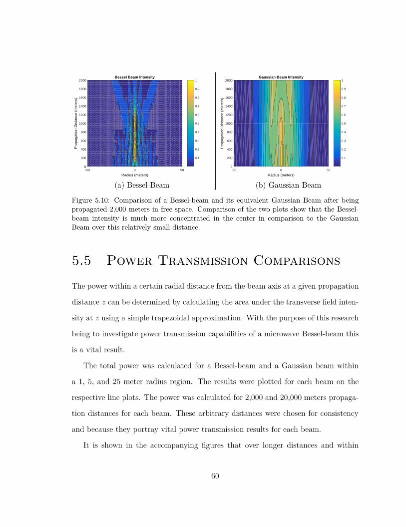
Figure 5.10: Comparison of a Bessel-beam and its equivalent Gaussian Beam after beingpropagated 2,000 meters in free space. Comparison of the two plots show that the Bessel-beam intensity is much more concentrated in the center in comparison to the GaussianBeam over this relatively small distance.
5.5 Power Transmission Comparisons
The power within a certain radial distance from the beam axis at a given propagation
distance z can be determined by calculating the area under the transverse field inten-
sity at z using a simple trapezoidal approximation. With the purpose of this research
being to investigate power transmission capabilities of a microwave Bessel-beam this
is a vital result.
The total power was calculated for a Bessel-beam and a Gaussian beam within
a 1, 5, and 25 meter radius region. The results were plotted for each beam on the
respective line plots. The power was calculated for 2,000 and 20,000 meters propaga-
tion distances for each beam. These arbitrary distances were chosen for consistency
and because they portray vital power transmission results for each beam.
It is shown in the accompanying figures that over longer distances and within
60

Bessel Beam Intensity
-50 0 50
Radius (meters)
0
0.2
0.4
0.6
0.8
1
1.2
1.4
1.6
1.8
2
Pro
paga
tion
Dis
tanc
e (m
eter
s)
×104
0.1
0.2
0.3
0.4
0.5
0.6
0.7
0.8
0.9
1
(a) Bessel-Beam
Gaussian Beam Intensity
-50 0 50
Radius (meters)
0
0.2
0.4
0.6
0.8
1
1.2
1.4
1.6
1.8
2
Pro
paga
tion
Dis
tanc
e (m
eter
s)
×104
0.1
0.2
0.3
0.4
0.5
0.6
0.7
0.8
0.9
1
(b) Gaussian Beam
Figure 5.11: Comparison of Bessel-beam and Gaussian Beam after being propagated 20,000meters in free space. Comparison of the two plots show that the Gaussian beam intensitydoes not decay nearly as fast as the Bessel-beam does in regards to distance propagated.
Bessel Beam Intensity
-300 -200 -100 0 100 200 300
Radius (meters)
0
1
2
3
4
5
6
7
8
9
10
Pro
paga
tion
Dis
tanc
e (m
eter
s)
×105
0
0.1
0.2
0.3
0.4
0.5
0.6
0.7
0.8
0.9
1
(a) Bessel-Beam
Gaussian Beam Intensity
-300 -200 -100 0 100 200 300
Radius (meters)
0
1
2
3
4
5
6
7
8
9
10
Pro
paga
tion
Dis
tanc
e (m
eter
s)
×105
0.1
0.2
0.3
0.4
0.5
0.6
0.7
0.8
0.9
1
(b) Gaussian Beam
Figure 5.12: Comparison of a Bessel-beam and Gaussian Beam after being propagated fromthe origin (1,000km above sea level) through the Earth’s atmosphere to sea level. In thissimulation both beams were truncated at the guard band (325 meters). As the beamstransitions from the ionized region to the non-ionized region they lose almost all of therebeam intensity.
61

Bessel Beam Intensity
-300 -200 -100 0 100 200 300
Radius (meters)
0
1
2
3
4
5
6
7
8
9
10P
ropa
gatio
n D
ista
nce
(met
ers)
×105
0
0.1
0.2
0.3
0.4
0.5
0.6
0.7
0.8
0.9
(a) Bessel-Beam
Gaussian Beam Intensity
-300 -200 -100 0 100 200 300
Radius (meters)
0
1
2
3
4
5
6
7
8
9
10
Pro
paga
tion
Dis
tanc
e (m
eter
s)
×105
0.1
0.2
0.3
0.4
0.5
0.6
0.7
0.8
0.9
1
(b) Gaussian Beam
Figure 5.13: Comparison of Bessel-beam and Gaussian Beam after being propagated fromthe origin (1,000km above sea level) through the Earth’s atmosphere to sea level. As theGaussian beam transitions from the ionized region to the non-ionized region it loses almostall of its beam intensity.
larger radial regions, the Gaussian beam delivers more power than does a truncated
Bessel-beam. The only instance where a Bessel-beam performs better then a Gaussian
beam is within a 1 meter radial region over propagation distances within the Bessel-
beams non-diffractive region.
62

0 200 400 600 800 1000 1200 1400 1600 1800 2000
Propagation Distance (meters)
0.2
0.3
0.4
0.5
0.6
0.7
0.8
0.9
1
1.1
1.2
Pow
er
Power Transmission within 1 Meter Region
Bessel BeamGaussian Beam
Figure 5.14: Comparison of a Bessel-beam and Gaussian beam power transmission quanti-ties within a 1 meter radius area over a propagation distance of 2,000 meters.
63

0 0.2 0.4 0.6 0.8 1 1.2 1.4 1.6 1.8 2
Propagation Distance (meters) ×104
0
0.2
0.4
0.6
0.8
1
1.2
Pow
er
Power Transmission within 1 Meter Region
Bessel BeamGaussian Beam
Figure 5.15: Comparison of a Bessel-beam and Gaussian beam power transmission quanti-ties within a 1 meter radius area over a propagation distance of 20,000 meters.
64

0 200 400 600 800 1000 1200 1400 1600 1800 2000
Propagation Distance (meters)
0.5
1
1.5
2
2.5
3
3.5
4
4.5
5
Pow
er
Power Transmission within 5 Meter Region
Bessel BeamGaussian Beam
Figure 5.16: Comparison of a Bessel-beam and Gaussian beam power transmission quanti-ties within a 5 meter radius area over a propagation distance of 2,000 meters.
65
0 0.2 0.4 0.6 0.8 1 1.2 1.4 1.6 1.8 2
Propagation Distance (meters) ×104
0
0.5
1
1.5
2
2.5
3
3.5
4
4.5
5
Pow
er
Power Transmission within 5 Meter Region
Bessel BeamGaussian Beam
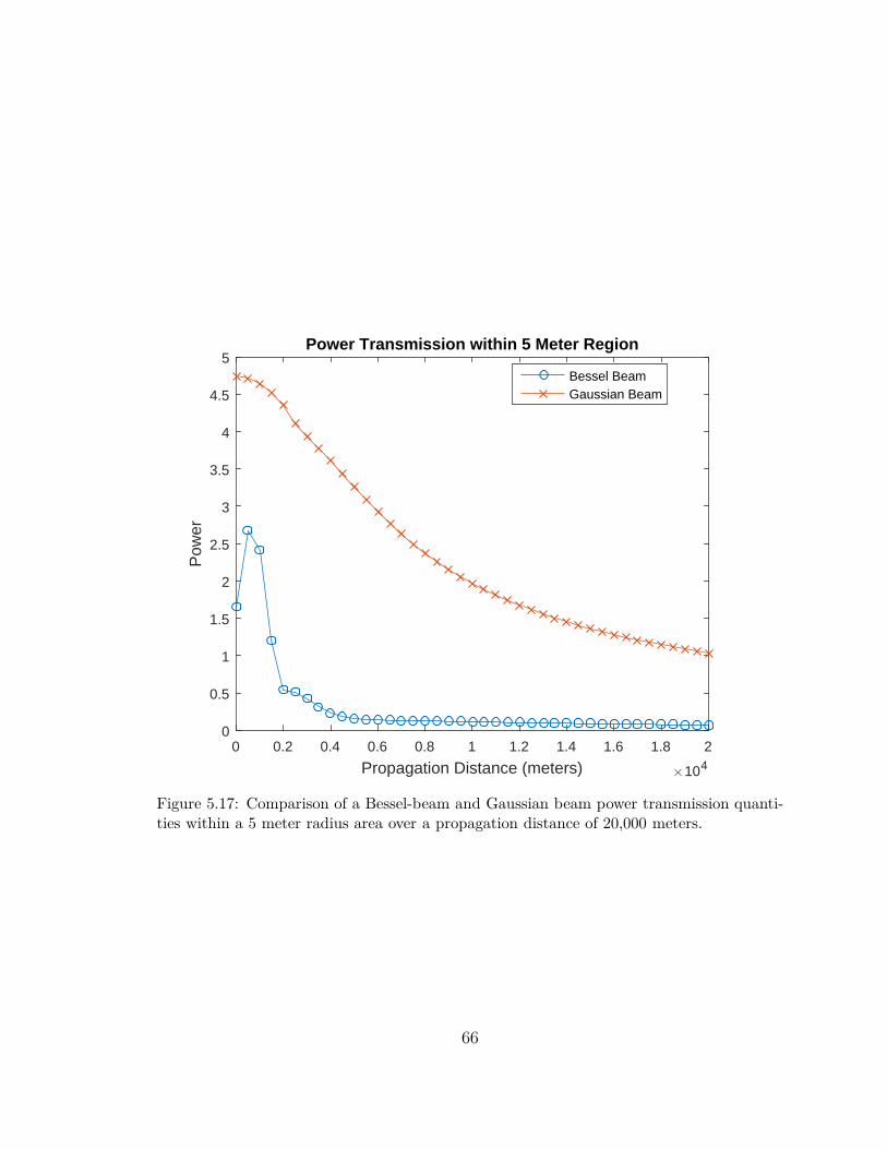
Figure 5.17: Comparison of a Bessel-beam and Gaussian beam power transmission quanti-ties within a 5 meter radius area over a propagation distance of 20,000 meters.
66

0 200 400 600 800 1000 1200 1400 1600 1800 2000
Propagation Distance (meters)
2
3
4
5
6
7
8
9
10
11
12
Pow
er
Power Transmission within 25 Meter Region
Bessel BeamGaussian Beam
Figure 5.18: Comparison of a Bessel-beam and Gaussian beam power transmission quanti-ties within a 25 meter radius area over a propagation distance of 2,000 meters.
67

0 200 400 600 800 1000 1200 1400 1600 1800 2000
Propagation Distance (meters)
2
3
4
5
6
7
8
9
10
11
12
Pow
er
Power Transmission within 25 Meter Region
Bessel BeamGaussian Beam
Figure 5.19: Comparison of a Bessel-beam and Gaussian beam power transmission quanti-ties within a 25 meter radius area over a propagation distance of 20,000 meters.
68

Chapter 6
Conclusions
The numerical results presented in this research lead to the following conclusions:
1. Propagation Properties through Free Space
(a) The Bessel-beam with an aperture radius equal to the guard band (325
meters) has a beam intensity more concentrated at the radial origin than
the equivalent size Gaussian beam over the same propagation distance.
The Gaussian beam also spreads faster than the Bessel-beam over the
same propagation distance.
(b) The Bessel-beam truncated at 25 meters has a beam intensity more con-
centrated at the radial origin than the Gaussian beam over a 2,000 meter
propagation distance. However, in this same instance the Bessel-beam
intensity rapidly decays to zero past approximately 2,000 meters. In com-
parison, the Gaussian beam maintains its beam intensity over this same
distance.
69

(c) In conclusion, a Bessel-beam with a 25 meter aperture would only be more
effective then a like Gaussian beam within its non-diffractive region in free
space.
2. Propagation Properties through a Spatially Inhomogeneous Medium
(a) The Bessel-beam truncated at the guard band (325 meters) has a beam
intensity that is more concentrated at the radial origin than the Gaussian
beam as they are propagated through the Earth’s atmosphere. The beam
intensity’s decay within the ionized region.
(b) In conclusion, propagation through the ionized region of the Earth’s at-
mosphere only causes both beams to decay more rapidly. Wireless power
transmission using either of these two beams through the Earth’s atmo-
sphere would not be efficient.
6.1 Future Research
Two things need to be done:
1. Small scale experiments.
2. More detailed calculations of atmospheric propagation.
70

References
[1] J. Durnin, “Exact solutions for nondiffracting beams. i. the scalar theory,”J. Opt. Soc. Am., 1987.
[2] N. Tesla, “Experimants with alternate currents of high potential and highfrequency,” in lecture before the Institution of Electrical Engineers.
[3] D. J. Griffiths, Introduction to Electrodynamics Fourth Edition. Pearson,2013.
[4] W. C. Brown, “Experimental airborne microwave supported platform,”tech. rep., Air Force Systems Command, 1965.
[5] R. M. Dickinson, “Evaluation of microwave high-power reception-conversion array for wireless power transmission,” tech. rep., National Aero-nautics and Space Administration, 1975.
[6] K. E. Oughstun, Electromagnetic and Optical Pulse Propagation 1 SpectralRepresentations in Temporally Dispersive Media. Springer, 2006.
[7] S. J. Robbins, “Elemental composistion of mars’ atmosphere,” tech. rep.,Case Western Reserve University Depeartment of Astronomy, 2006.
[8] K. A. Dao, V. P. Tran, and C. D. Nguyen, “The wireless transmissionenvironment from geo to the earth and numerical estimation of relativepermittivity vs the altitude in the neutral and ionized layers of the earthatmosphere,” in Proceeding of The 2014 International Conference on Ad-vanced Technologies for Communications (ATC-14).
[9] R. A. Chipman, Schaum’s Outline of Theory and Problems of TransmissionLines. McGraw-Hill, 1968.
[10] K. T. McDonald, “Bessel beams,” tech. rep., Joseph Henry Laboratories,Priceton University, 2000.
[11] M. Anguiano-Morales, “Generation of a spiral wave by modified annularslit,” Opt. Eng. 50(7), 2011.
[12] E. W. Weisstein, “Hankel transform,” tech. rep., From MathWorl–A Wol-fram Web Resource, 2016.
[13] A. E. Seigman, “Quasi fast hankel transform,” Opt. Lett. 1, 13, 1977.
71

Appendix A
Hankel Transform
The Hankel transform is derived here from the 2D-Fourier transform in (x, y) coordi-
nates through a coordinate change to polar coordinates (r, θ). The Hankel transform
of order zero is an integral transform equivalent to a 2D-Fourier transform with a
radially symmetric integral kernel. This is defined as [12]
g(u, v) =∫
∞
−∞
∫∞
−∞
f(r)e−2πi(ux+vy)dxdy. (A.1)
Let
x+ iy = reiθ, (A.2)
and
u+ iv = qeiφ, (A.3)
so that x = r cos θ, y = r sin θ, where
r =√
x2 + y2, (A.4)
72

and u = q cosφ, v = q sin φ, where
q =√u2 + v2. (A.5)
Then
g(q) =∫
∞
0
∫ 2π
0f(r)e−2πirq cos θrdrdθ (A.6)
so that
g(q) = 2π∫
∞
0f(r)J0(2πqr)rdr (A.7)
where J0(z) is the zeroth order Bessel function of the first kind.
A.1 Quasi-Fast Hankel Transform
Testing the Quasi-fast Hankel transform (QFHT) was necessary in order to prove it
yields correct results when applied to the Bessel-beam. This was done by comparing
the results of two different mathematical procedures performed on specific functions.
One mathematical procedure being the integration of the zeroth order Bessel function
and the other performing the QFHT on the unit step function. If the QFHT is working
properly these will yield the same results, possibly with some correction constant.
The Hankel transform of the circle function f(r) = 1 for r ≤ 1 and f(r) = 0 for
r > 0 is given by
2π∫ 1
0J0(2πkr)rdr = 2π
J1(2πk)
2πk(A.8)
where the limits 0 and 1 in the integral are determined by the Hankel transform itself
(the lower bound) and by the circle function (both lower and upper bounds). The
73

code used to perform the QFHT is shown below:
1 % Quasi-Fast Hankel Transform
2 K = w/c0; % maximum spatial frequency
3 R = 25; % maximum radius
4 n=0;
5 M=7;
6 m=5;
7 a=K*R/2/pi;
8 N=pow2(ceil(1 + log2(a*m*log(a*M))));
9 a=1/a/m;
10 ro=R*exp(-a*N/2);
11 ko=K*exp(-a*N/2);
12 I=exp(a*(0:N-1));
13 k=ko*I(1:N/2); % samplings
14 r=ro*I(1:N/2);
15 I=ifft(a*ko*ro*I.*besselj(n,ko*ro*I)); % kernel
16
17 h = [ones(1,4900), zeros(1,3292)]; % unit step function
18
19 H=fft(fft(h.*r,N).*I); % transform
20 H=real(H);
21 H=2*pi*H(1:N/2)./k;
A radial plot of the unit circle function is shown in Fig. A.1. Using the resulting
spatial frequency (k) values computed in the algorithm the QFHT calculation of
the spectrum (H) of this unit circle function can then be compared to the analytic
integration result given in Eq. A.7 in order to demonstrate its degree of accuracy.
The comparison is given in Fig. A.2. The zeroes of the Bessinc function in Eq. (A.8)
occur at the zeroes of the J1(ρ) Bessel function excluding the zero at the origin. A
comparison of the zeroes for the QFHT calculation with these analytic values along
with the accompanying percent differences are given in table A.1, showing that the
error is below 0.5%.
74
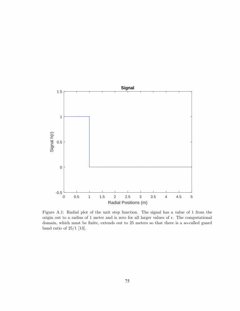
0 0.5 1 1.5 2 2.5 3 3.5 4 4.5 5
Radial Positions (m)
-0.5
0
0.5
1
1.5
Sig
nal h
(r)
Signal
Figure A.1: Radial plot of the unit step function. The signal has a value of 1 from theorigin out to a radius of 1 meter and is zero for all larger values of r. The computationaldomain, which must be finite, extends out to 25 meters so that there is a so-called guardband ratio of 25/1 [13].
75

0 1 2 3 4 5 6 7 8 9
Spatial Frequency (cycles/m)
-0.5
0
0.5
1
1.5
2
2.5
3
3.5
Spe
ctru
m H
(k)
Numerical Verification of QFHT
IntegrationQFHT
Figure A.2: Plot depicting the results and comparison of the QFHT to direct integration. Itis seen that the integration results overlap the QFHT results. A comparison of the QFHTzeros the the integration zeros along with the percent difference are given in table A.1. Thenonlinear radial spacing used in the QFHT is equivalent in the figure
76

Table A.1: Zeroes Comparison
nJ1(xn) = 0
xn
Integrationxn/2π
QFHTPercent
Difference1 3.832 0.609835 0.612349 0.411388%2 7.016 1.116565 1.121391 0.431275%3 10.173 1.619158 1.625748 0.406191%4 13.323 2.120531 2.129798 0.436083%5 16.470 2.621382 2.631958 0.402637%6 19.612 3.121961 3.135691 0.438819%7 22.760 3.62238 3.636885 0.399629%8 25.903 4.122697 4.140943 0.44158%9 29.047 4.622971 4.641339 0.396529%10 32.190 5.123147 5.145943 0.443984%11 35.332 5.623311 5.645556 0.394805%12 38.475 6.123449 6.150828 0.446118%13 41.617 6.623566 6.649634 0.392786%14 44.759 7.123667 7.155656 0.448054%15 47.901 7.623754 7.653616 0.390922%
77

Appendix B
Microwave Bessel-Beam
Propagation
In order to create the plane wave spectrum representation of a microwave Bessel-
beam, several specific steps need to be taken. Because the radial component of the
electric field, given by
Eρ = cosαJ1(kρ sinα)ei(kz cos α−ωt) (B.1)
is the focus of this research, numerical values for the initial beam parameters must
first be defined. The angle (α) and radius (r) of the aperture were chosen to be 1
degree and 25 meters, respectively. The frequency of the beam was chosen to be
2.45 GHz. The wave number can then be calculated from these values. The code
implementing these mathematical steps is given below:
1 % Initial Beam Parameters
2 c0 = 299792458; % speed of light in a vacuum
3 f = 2.45*10^9; % microwave frequency
78
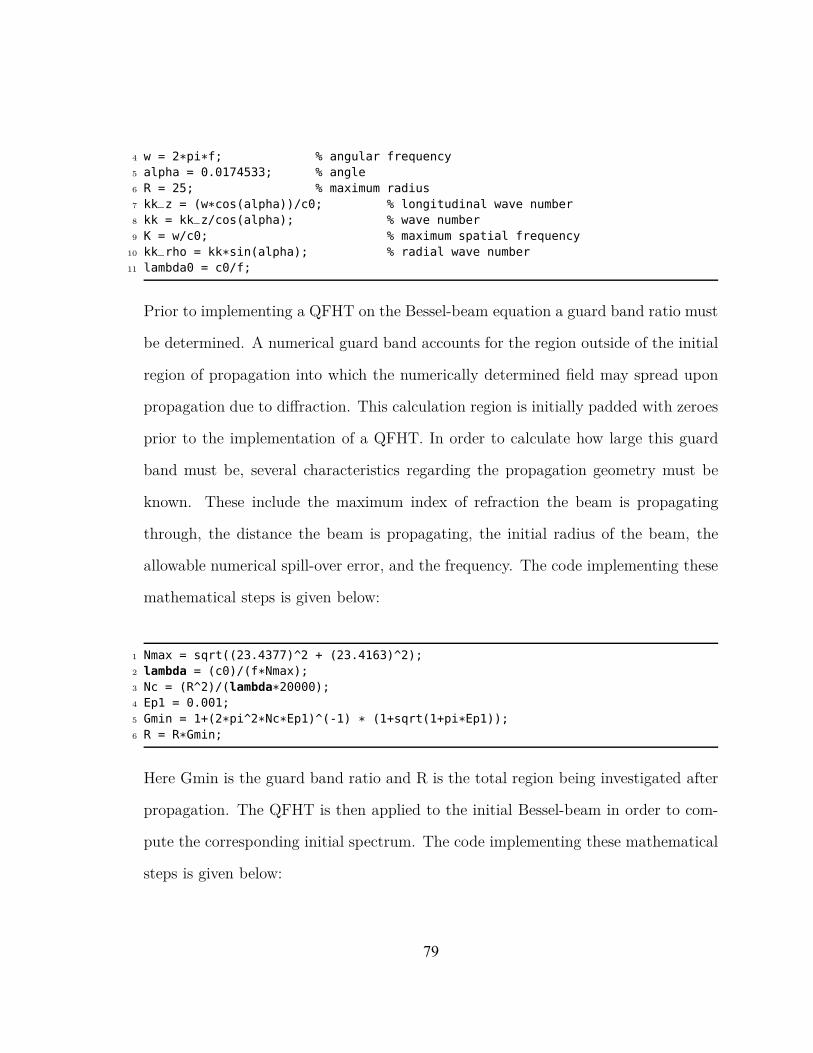
4 w = 2*pi*f; % angular frequency
5 alpha = 0.0174533; % angle
6 R = 25; % maximum radius
7 kk_z = (w*cos(alpha))/c0; % longitudinal wave number
8 kk = kk_z/cos(alpha); % wave number
9 K = w/c0; % maximum spatial frequency
10 kk_rho = kk*sin(alpha); % radial wave number
11 lambda0 = c0/f;
Prior to implementing a QFHT on the Bessel-beam equation a guard band ratio must
be determined. A numerical guard band accounts for the region outside of the initial
region of propagation into which the numerically determined field may spread upon
propagation due to diffraction. This calculation region is initially padded with zeroes
prior to the implementation of a QFHT. In order to calculate how large this guard
band must be, several characteristics regarding the propagation geometry must be
known. These include the maximum index of refraction the beam is propagating
through, the distance the beam is propagating, the initial radius of the beam, the
allowable numerical spill-over error, and the frequency. The code implementing these
mathematical steps is given below:
1 Nmax = sqrt((23.4377)^2 + (23.4163)^2);
2 lambda = (c0)/(f*Nmax);
3 Nc = (R^2)/(lambda*20000);
4 Ep1 = 0.001;
5 Gmin = 1+(2*pi^2*Nc*Ep1)^(-1) * (1+sqrt(1+pi*Ep1));
6 R = R*Gmin;
Here Gmin is the guard band ratio and R is the total region being investigated after
propagation. The QFHT is then applied to the initial Bessel-beam in order to com-
pute the corresponding initial spectrum. The code implementing these mathematical
steps is given below:
79

1 % Define electric field equation
2 h=@(r)( cos(alpha).*besselj(1,r*kk*sin(alpha)) );
3
4 n=0;
5 M=7;
6 m=5;
7
8 a=K*R/2/pi;
9 N=pow2(ceil(1 + log2(a*m*log(a*M))));
10 a=1/a/m;
11 ro=R*exp(-a*N/2);
12 ko=K*exp(-a*N/2);
13 I=exp(a*(0:N-1));
14 k=ko*I(1:N/2); % samplings
15 r=ro*I(1:N/2);
16 I=ifft(a*ko*ro*I.*besselj(n,ko*ro*I)); % kernel
17 h=feval(h,r);
18 h = h(1:end-34000);
19 h = [h, zeros(1,34000)]; % zero padding guard band
20 H=fft(fft(h.*r,N).*I); % transform
21 H=real(H);
22 H=2*pi*H(1:N/2)./k;
23
24 k = k./(2*pi);
Once the initial spectrum has been computed, the beam spectrum is then propagated
a specific distance ∆z=dis through the medium with index of refraction (nc) through
multiplication by the exponential factor e(iβ∆z). An example of this calculation for a
distance of 1,000 meters is provided in the code below:
1 lambda = lambda0/n_c(1);
2 beta = (2*pi/real(lambda))*(1-real(lambda)^2.*k.^2).^(1/2);
3 alpha = 1i*((2*pi/imag(lambda))*(1-imag(lambda)^2.*k.^2).^(1/2));
4 Beta = beta + alpha;
5 dis = 1000;
6 H = H.*exp(1i*Beta*dis);
This propagation process then results in an altered spectrum. The IQFHT is then
applied to this propagated beam spectrum, resulting in the propagated field at the
specified distance.
80
Recommended
![Propagation of Bessel and Airy beams through atmospheric ... · modify the propagation of laser beams through atmosphere [1-7]. In weak atmospheric turbulence, the modifications can](https://img.pdfslide.net/doc/110x75/5f30f0d7fc73d56e2278b679/propagation-of-bessel-and-airy-beams-through-atmospheric-modify-the-propagation.jpg)