Sengupta, M. and Dalwani, R. (Editors). 2008 Proceedings of Taal2007: The 12th World Lake Conference: 799-811

Modelling the Eutrophication Sven Erik Jørgensen, Copenhagen University, Institute A, Environmental Chemistry Section, University Park 2, 2100 Copenhagen Ø, Denmark Email: sej@farma.ku.dk

ABSTRACT After a short overview of the spectrum of eutrophication models available to day, three core submodels are discussed. The three submodels are considered in all models with a medium to high complexity. The data requirement to develop a model with a medium to high complexity is discussed. It is possible to conclude that reasonable reliable prognoses can be developed by eutrophication models to day, provided that a reasonable good data base is available. The challenge of modelling the biomanipulation is discussed and the conclusion is that structurally dynamic models can explain the success and failure of biomanipulation. A general use of structurally dynamic models is discussed and particularly for eutrophication modelling they offer a good solution to the problem associated with development of reliable prognoses. It is also recommended to use the structurally dynamic approach by calibration of eutrophication models as most lakes have a seasonal shift in the species composition.

INTRODUCTION: Model Overview Eutrophication models represent a particularly wide spectrum of complexity. Table 1 reviews various eutrophication models representing the spectrum of complexity and the characteristics of the models (i.e., the number of state variables, the nutrients considered, the number of lake segments or number of water layers, whether constant stoichiometric or independent nutrient cycles were applied, whether the model has been calibrated and validated, the number of case studies to which the model has been applied, etc.). The table is far from being complete, but give a good overview of spectrum of model complexity. It is assumed, particularly for more complex models, that some modifications from case to case to reflect specific lake conditions or properties should be reflected in the model.

The simple calculation modelling approach is exemplified by the relation between phosphorus, which can easily be calculated on the basis of the relation between the phosphorus load (corrected by the fraction trapped in the sediment) and chlorophyll. (e.g., see OECD, 1982; Ryding and Rast, 1989; Rast and Thornton, 1996). Such empirical relations do have shortcomings They are far from being general and, therefore, should be used with proper caution. The differences between the various empirical relationships indicates that a high standard deviation can be expected by application of empirical relationships.

As seen in Table 1, the dynamic models represent a wide range of complexity, given that the different models include a different number of sub-models. Three possible core sub-models that should be considered for inclusion in models of medium to

high complexity are presented below. The characteristics of each case study should determine whether these three sub-models should be included or not and with which complexity. They represent typical considerations for selecting the complexity for eutrophication models. Three important submodels For the medium and complex eutrophication models particularly three submodels are usually under discussion. The three submodels are:

1) phytoplankton growth with or without independent nutrient cycling

2) sediment water exchange of nutrients 3) grazing and predation

1) The application of independent nutrient cycles inevitably increases the complexity of a model, as this situation requires that nitrogen, phosphorus, carbon and perhaps silica may be included as state variables in each trophic level. In most models that include independent nutrient cycles, however, only one state variable is considered for zooplankton and fish. The application of independent nutrient cycles implies that the growth of phytoplankton is described as a two-step process, as follows: • Phytoplankton nutrient uptake, in accordance

with Monod's kinetics, • Phytoplankton growth determined by the

internal substrate concentration. This complication obviously requires that the

underlying data are of sufficient quality and quantity. Di Toro (1980) has shown that the application of independent nutrient cycles is particularly important when the model is used for shallow, very eutrophic lakes. In contrast, this complication can be omitted for deep, mesotrophic or oligotrophic lakes.

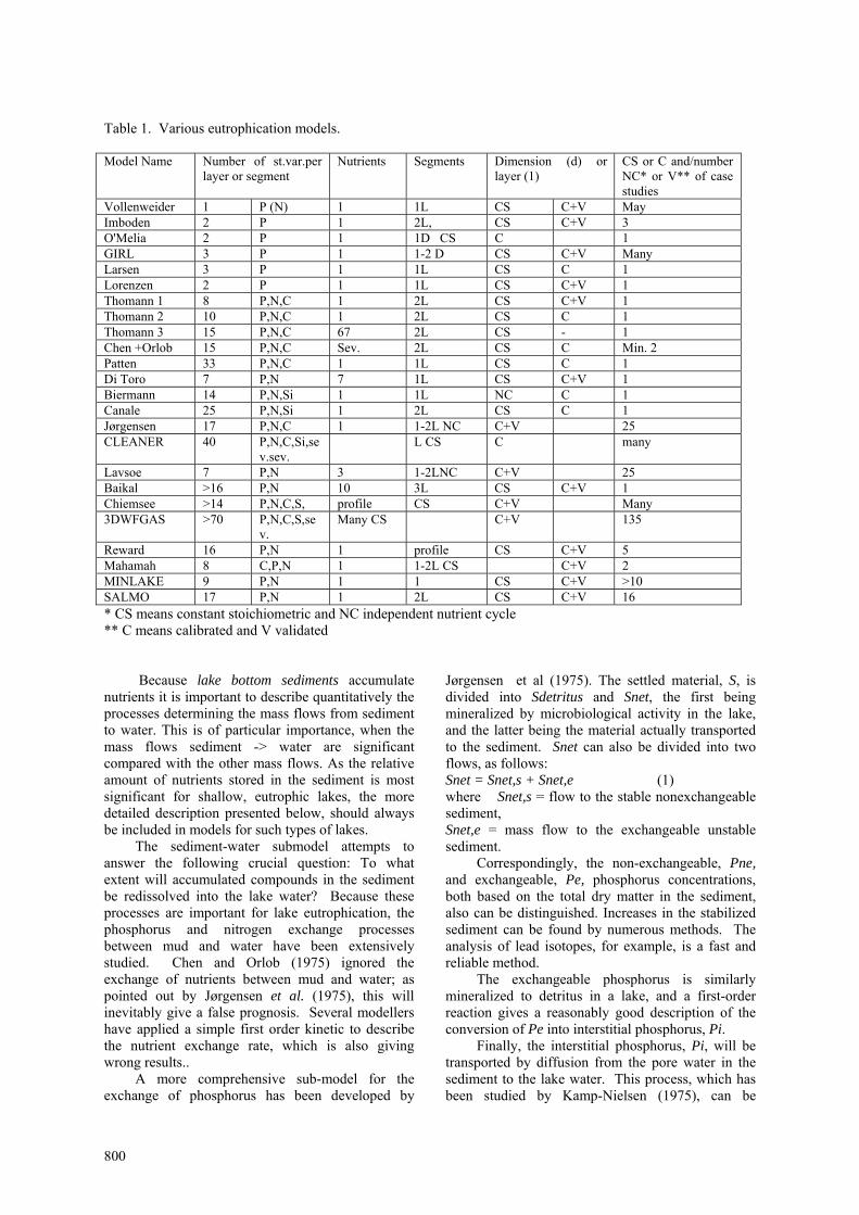
Table 1. Various eutrophication models. Model Name Number of st.var.per

layer or segment Nutrients Segments Dimension (d) or

layer (1) CS or C and/number NC* or V** of case studies

Vollenweider 1 P (N) 1 1L CS C+V May Imboden 2 P 1 2L, CS C+V 3 O'Melia 2 P 1 1D CS C 1 GIRL 3 P 1 1-2 D CS C+V Many Larsen 3 P 1 1L CS C 1 Lorenzen 2 P 1 1L CS C+V 1 Thomann 1 8 P,N,C 1 2L CS C+V 1 Thomann 2 10 P,N,C 1 2L CS C 1 Thomann 3 15 P,N,C 67 2L CS - 1 Chen +Orlob 15 P,N,C Sev. 2L CS C Min. 2 Patten 33 P,N,C 1 1L CS C 1 Di Toro 7 P,N 7 1L CS C+V 1 Biermann 14 P,N,Si 1 1L NC C 1 Canale 25 P,N,Si 1 2L CS C 1 Jørgensen 17 P,N,C 1 1-2L NC C+V 25 CLEANER 40 P,N,C,Si,se

v.sev. L CS C many

Lavsoe 7 P,N 3 1-2LNC C+V 25 Baikal >16 P,N 10 3L CS C+V 1 Chiemsee >14 P,N,C,S, profile CS C+V Many 3DWFGAS >70 P,N,C,S,se

v. Many CS C+V 135

Reward 16 P,N 1 profile CS C+V 5 Mahamah 8 C,P,N 1 1-2L CS C+V 2 MINLAKE 9 P,N 1 1 CS C+V >10 SALMO 17 P,N 1 2L CS C+V 16 * CS means constant stoichiometric and NC independent nutrient cycle ** C means calibrated and V validated

Because lake bottom sediments accumulate

nutrients it is important to describe quantitatively the processes determining the mass flows from sediment to water. This is of particular importance, when the mass flows sediment -> water are significant compared with the other mass flows. As the relative amount of nutrients stored in the sediment is most significant for shallow, eutrophic lakes, the more detailed description presented below, should always be included in models for such types of lakes.

The sediment-water submodel attempts to answer the following crucial question: To what extent will accumulated compounds in the sediment be redissolved into the lake water? Because these processes are important for lake eutrophication, the phosphorus and nitrogen exchange processes between mud and water have been extensively studied. Chen and Orlob (1975) ignored the exchange of nutrients between mud and water; as pointed out by Jørgensen et al. (1975), this will inevitably give a false prognosis. Several modellers have applied a simple first order kinetic to describe the nutrient exchange rate, which is also giving wrong results..

A more comprehensive sub-model for the exchange of phosphorus has been developed by

Jørgensen et al (1975). The settled material, S, is divided into Sdetritus and Snet, the first being mineralized by microbiological activity in the lake, and the latter being the material actually transported to the sediment. Snet can also be divided into two flows, as follows: Snet = Snet,s + Snet,e (1) where Snet,s = flow to the stable nonexchangeable sediment, Snet,e = mass flow to the exchangeable unstable sediment.

Correspondingly, the non-exchangeable, Pne, and exchangeable, Pe, phosphorus concentrations, both based on the total dry matter in the sediment, also can be distinguished. Increases in the stabilized sediment can be found by numerous methods. The analysis of lead isotopes, for example, is a fast and reliable method.

The exchangeable phosphorus is similarly mineralized to detritus in a lake, and a first-order reaction gives a reasonably good description of the conversion of Pe into interstitial phosphorus, Pi.

Finally, the interstitial phosphorus, Pi, will be transported by diffusion from the pore water in the sediment to the lake water. This process, which has been studied by Kamp-Nielsen (1975), can be

800

described by means of the following empirical equation (valid at 7°C): Phosphorus release = 1.21 (Pi - Ps) - 1.7 (mg P/m2.day) (2) where Ps = the dissolved phosphorus in the lake water.

This submodel of water-sediment exchange was validated in three case studies (Jørgensen et al., 1975), based on examining sediment cores in the laboratory. Kamp-Nielsen (1975) has added an adsorption term to these equations.

A similar sub-model for sediment nitrogen release has been developed by Jacobsen and Jørgensen (1975). The nitrogen release from sediment is expressed as a function of the nitrogen concentration in the sediment and the temperature, under both aerobic and anaerobic conditions.

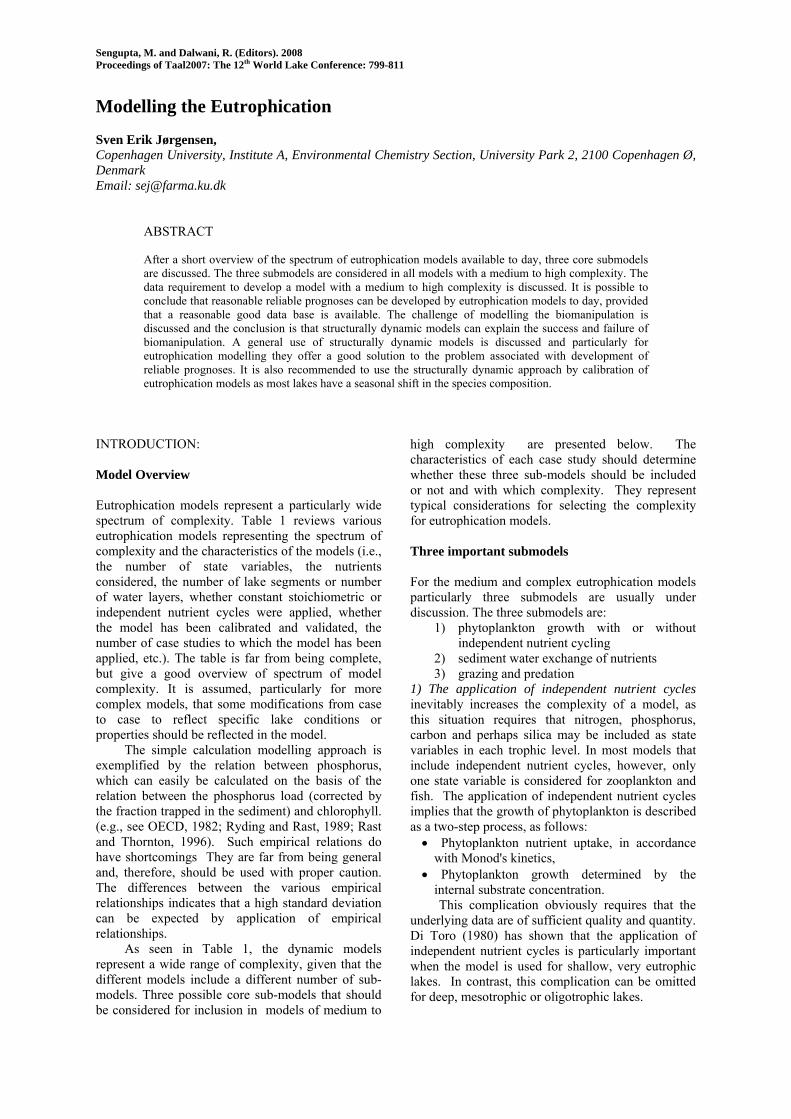
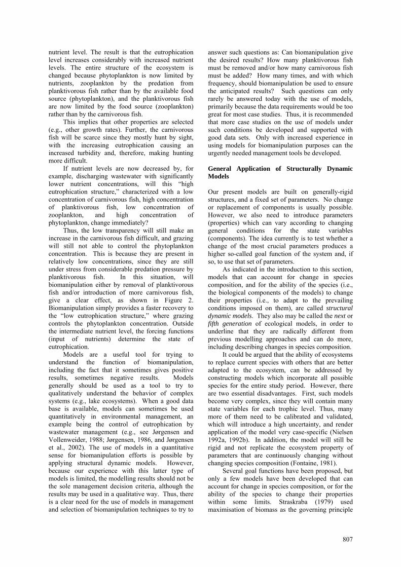
Figure 1 shows a sediment profile from these examinations, illustrating the interpretation of the profile that can be used in the model to distinguish between exchangeable and non-exchangeable sediment phosphorus.

+++

+

+

+

+

+

+

+

A B

LUL

0

5

10

15

0 1 2 3 4 5 6

g P / kg D:M:

Dep

th (

cm)

C

Figure 1. Analysis of sediment core from Lake Esrom. Phosphorus concentration (mg P/g dry matter) is plotted against the depth. The area C represents exchangeable phosphorus. The fraction of exchangeable P to total P at the sediment surface = (B / (B+A)), LUL is the unstabilized layer.

Grazing of phytoplankton by zooplankton (Z), and the predation of zooplankton by fish (F) are both expressed by a modified Monod expression, which considers a threshold concentration, KT, below which grazing or the predation does not occur. The expression for phytoplankton grazing by zooplankton (Steele, 1974) is expressed as follows: µZ = µZmax . (Phyt -KT) / (Phyt + KM) (3) where KM = Michaelis-Menten constant.

A zooplankton carrying-capacity often must be

introduced to give a better simulation of zooplankton and phytoplankton. Although carrying capacities are often observed in ecosystems, the need to introduce them in this case may be due to a too-simple representation of the grazing process. Phytoplankton might not be grazed, for example, by all the zooplankton species present, and some zooplankton species might use detritus as a food source. The zooplankton growth rate, mZ, is computed in accordance with these modifications as: µZ = µZmax . FPH . FT2 . F2CK (4) where FPH = the expression in equation (5.4), FT2 = a temperature regulation expression, F2CK = accounts for the carrying capacity,

Now, F2CK = (CK - ZOO) / CK (5) where CK = carrying capacity.

Data If the data are not sufficient to include the three important sub-models presented above, or other relevant sub-models, that an individual case study might require, it is recommended that the needed data be obtained with an intensive measuring effort that can provide high-quality data for the specific time period when the eutrophication processes are most dynamic.

An intensive measuring period, with several sets of measurements each week during the spring and summer bloom period, can first of all be applied to improve parameter estimation, which is often a focal problem in developing ecological models. The experience from conducting intensive measuring periods has identified the following advantages :

• Different optional expressions of simultaneously-limiting factors were tested, and only two gave an acceptable maximum growth rate for phytoplankton and an acceptable low standard deviation. These were (i) multiplication of the limiting factors, and (ii) averaging the limiting factors.

• The previously applied expression for the influence of temperature on phytoplankton growth gave unacceptable parameters, with standard deviations that were too high. A better expression (Equation 1) was introduced as a result of the intensive measuring period.

• It was possible to improve the parameter estimation, which gives more realistic values for some parameters. Whether this would give an improved validation when observations from a period with drastic changes in the nutrients loading are available could not be determined.

• The other expressions applied for process descriptions were confirmed.

Validation

801

It is important to validate models against independent set of measurements. Table 2 gives the results of a typical validation for a model with a medium to high complexity, developed on basis of good data. R and A are the standard deviations for the mean and maximum value, respectively, of the considered state variables. Y, R and A give the errors in relative terms. Multiplying them by 100 gives the errors expressed as percentages (%). As shown in the table, the standard deviation, Y, for all measured state variables is 16%. It is the standard deviation for one comparison of modelled and measured values. As the standard deviation for a comparison of n sets of modelled and measured values is ûn times smaller, and n is in the order of 200, the average picture of the lake is provided, with a very acceptable standard deviation of about 1%. Y is generally 5-10 times larger, for example, for hydrological models (WMO, 1975). Table 2. Numerical validation of the described model. Validation Criterion

State Variable Value

Y all 0.16 R Ptotal 0.18 R Psoluble 0.16 R Ntotal 0.02 R Nsoluble 0.14 R Phytoplankton 0.08 R Zooplankton 0.20 R Production 0.03 A Ptotal 0.12 A Psoluble 0.15 A Ntotal 0.07 A Nsoluble 0.03 A Phytoplankton 0.15 A Zooplankton 0.00 A Production 0.08

The relative errors of the mean values, R, are 3% for production, 8% for phytoplankton and 2% for nitrogen, all of which are very acceptable values. The relative error for total phosphorus, however, is 18%, and that for zooplankton is 20%, both of which must be considered as being too large. The relative errors of the maximum values, A, range from 0% to 15%, an acceptable range. The ability of the model to predict maximum production and maximum phytoplankton concentrations has special interest within the context of a eutrophication model, with the relative errors being 8% and 15%, respectively – both of which are very acceptable. Prognoses A prognosis for the development of eutrophication in Lake Glumsø (the validation results referred to in

Table 2 are based on this case study) by different removal efficiencies for phosphorus, nitrogen, or phosphorus and nitrogen simultaneously, have been made. The validation of this prognosis is presented here to illustrate the reliability of prognoses made on the basis of well-developed eutrophication models.

It was previously stated that nitrogen removal had little or no effect on the lake, while phosphorus removal would give substantial reductions in the phytoplankton concentration. The results of two cases are summarized in Table 3, as follows:

Case A: The treated waste water has a concentration of 0.4 mg P/L, corresponding to about 92% removal efficiency, which should be achieved with proper chemical precipitation.

Case B: The treated wastewater has a concentration of 0.1 mg P/L, corresponding to about 98% removal efficiency, which will require chemical precipitation, for example, in combination with ion exchange.

As seen in Table 3, the water quality will improve significantly, in accordance with the predictions. Case B, with a 98% removal of phosphorus, is obviously preferred. In the third year, Case B will give a reduction in production from 1,100 g C/m2.yr to 500 g C/m2.yr, with the water transparency increasing from a minimum value of 20 - 60 cm. The 9th year would even result in reduction of the production to 320 g C/m2.yr, corresponding to a mesotrophic lake, which is an acceptable improvement for a shallow lake situated in an agricultural area. Table 3. Model predictions in two cases for concentrations of treated wastewater: Case A: 0.4 mg P/L; Case B: 0.1 mg P/L.

THIRD YEAR NINTH YEAR Case A Case B Case A

Case B

g C/m2.yr 650 500* 500 320* Minimum transparency (cm)

50 60 60 75

* an error of 3% on this value could be expected if the validation results hold, see R for production in Table 5.7.

The prognosis gives a pronounced effect of 98% phosphorus removal, which could therefore be recommended to the appropriate environmental authorities. Further improvements after nine years should not be expected with this case study.

Conveyance of the wastewater also was considered, but has the following disadvantages:

• It is slightly more expensive than the Case B solution, taking interests, depreciation and running costs into consideration,

• The phosphorus is not removed but only transported to the downstream Susaa River, where its effects not have been considered,

802

• The sludge produced at the biological treatment plant will be less valuable as a soil conditioner, since the phosphorus concentration will be lower than when phosphorus removal is included.

• The freshwater is not retained in the lake, from which it could have been reclaimed, if needed, after storage for some time. Freshwater is not presently a problem in this area, but it is foreseen that it might be in 20 - 40 years.

In spite of these observations, the community in this case study chose to convey its wastewater to the Susaa River, due to a preference for traditional methods. The pipeline was constructed in 1980 and began operation in April 1981, which has enabled a validation of the presented prognosis.

Lake Glumsø was ideal for these studies due to its limited depth and size, but also because a reduced nutrient input to the lake could be foreseen. The limited retention time (about six months) makes it realistic to obtain a validation of a prognosis within a relatively short time interval (a few years). On April 1, 1981, the direct input of wastewater to the lake was stopped. Because the capacity of the sewage system is still too small, however, a minor input of mixed rain water and wastewater is discharged into the lake from time to time through an upstream tributary. Thus, the phosphorus loading is not reduced by 98%, but rather only by 88% (determined by a phosphorus balance). The prognosis in Case A, therefore, can be used for comparison.

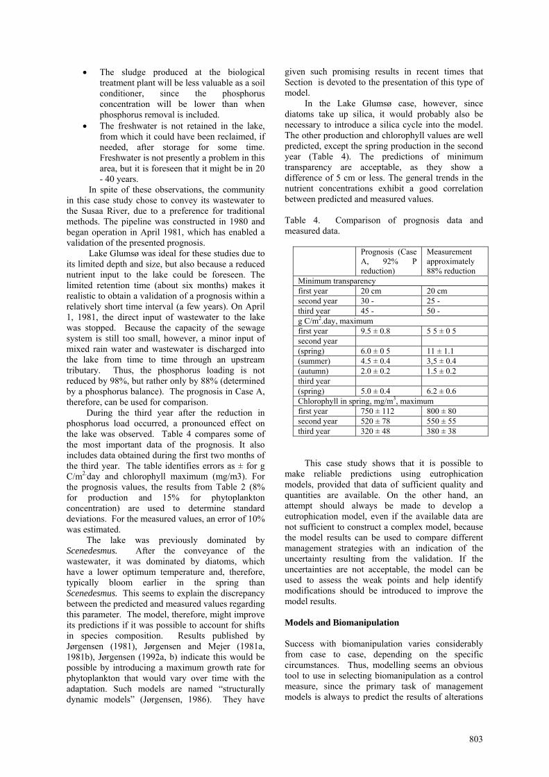
During the third year after the reduction in phosphorus load occurred, a pronounced effect on the lake was observed. Table 4 compares some of the most important data of the prognosis. It also includes data obtained during the first two months of the third year. The table identifies errors as ± for g C/m2.day and chlorophyll maximum (mg/m3). For the prognosis values, the results from Table 2 (8% for production and 15% for phytoplankton concentration) are used to determine standard deviations. For the measured values, an error of 10% was estimated.

The lake was previously dominated by Scenedesmus. After the conveyance of the wastewater, it was dominated by diatoms, which have a lower optimum temperature and, therefore, typically bloom earlier in the spring than Scenedesmus. This seems to explain the discrepancy between the predicted and measured values regarding this parameter. The model, therefore, might improve its predictions if it was possible to account for shifts in species composition. Results published by Jørgensen (1981), Jørgensen and Mejer (1981a, 1981b), Jørgensen (1992a, b) indicate this would be possible by introducing a maximum growth rate for phytoplankton that would vary over time with the adaptation. Such models are named “structurally dynamic models” (Jørgensen, 1986). They have

given such promising results in recent times that Section is devoted to the presentation of this type of model.

In the Lake Glumsø case, however, since diatoms take up silica, it would probably also be necessary to introduce a silica cycle into the model. The other production and chlorophyll values are well predicted, except the spring production in the second year (Table 4). The predictions of minimum transparency are acceptable, as they show a difference of 5 cm or less. The general trends in the nutrient concentrations exhibit a good correlation between predicted and measured values. Table 4. Comparison of prognosis data and measured data.

Prognosis (Case A, 92% P reduction)

Measurement approximately 88% reduction

Minimum transparency first year 20 cm 20 cm second year 30 - 25 - third year 45 - 50 - g C/m2.day, maximum first year 9.5 ± 0.8 5 5 ± 0 5 second year (spring) 6.0 ± 0 5 11 ± 1.1 (summer) 4.5 ± 0.4 3,5 ± 0.4 (autumn) 2.0 ± 0.2 1.5 ± 0.2 third year (spring) 5.0 ± 0.4 6.2 ± 0.6 Chlorophyll in spring, mg/m3, maximum first year 750 ± 112 800 ± 80 second year 520 ± 78 550 ± 55 third year 320 ± 48 380 ± 38

This case study shows that it is possible to make reliable predictions using eutrophication models, provided that data of sufficient quality and quantities are available. On the other hand, an attempt should always be made to develop a eutrophication model, even if the available data are not sufficient to construct a complex model, because the model results can be used to compare different management strategies with an indication of the uncertainty resulting from the validation. If the uncertainties are not acceptable, the model can be used to assess the weak points and help identify modifications should be introduced to improve the model results.

Models and Biomanipulation Success with biomanipulation varies considerably from case to case, depending on the specific circumstances. Thus, modelling seems an obvious tool to use in selecting biomanipulation as a control measure, since the primary task of management models is always to predict the results of alterations

803

804

in an ecosystem. However, biomanipulation implies that the structure of the ecosystem (i.e., a lake) is changed, which is much more difficult to similate with a model than is a simple change in forcing functions. On the other hand, structural dynamic models are emerging (e.g., see Jørgensen, 1992a, 1992b). Models are increasingly used as an experimental tool that can sometimes also be used to explain ecosystem behaviour (Jørgensen 1992b) associated, for example, with chaos and catastrophe theories.

Models based on case studies with structural changes are still rare. However, we know that ecosystems have the ability to adapt to changed forcing functions, and to shift to species better suited to emerging conditions. Because radical changes are imposed on ecosystems, which inevitably will lead to the most pronounced changes in ecosystem structures, it is particularly interesting to apply models with dynamic structures, which are becoming increasingly important in environmental management. Thus, this type of model is discussed in this section in relation to lake and reservoir biomanipulation.

Biomanipulation is based on changes in ecosystem structure imposed by intentional changes in fish populations. In this context, it is of interest to explain when and why top-down control measures are working (i.e., when the imposed structural

changes can be predicted to work). This is also possible with the use of catastrophe theory on lake eutrophication models.

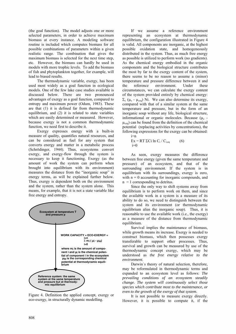
The short-term results of biomanipulation have been encouraging. It is unclear, however, whether or not a manipulated ecosystem will ultimately return to the initial eutrophic and turbid conditions. Some observations suggest that, if low nutrient concentrations are combined with a relatively high concentration of predatory fish, a stable steady state will be attained, while high nutrient concentration and high predatory concentration will lead to an unstable clear water state (see Hosper, 1989; Van Donk et al., 1989). On the other hand, turbid conditions may prevail even at medium nutrient concentrations, provided that the predatory fish concentration is low. By introducing more predatory fish, however, the conditions may improve significantly, even at medium nutrient concentrations. Willemsen (1980) distinguishes in the temperate region into two possible conditions: • A “bream state,” characterized by turbid water,

and a high degree of eutrophication relative to the nutrient concentration. Submerged vegetation is largely absent from such systems. Large amounts of bream are found, while pike are rarely found.

Nutrient concentration

Phy

topl

ankt

on c

onc.

or

prim

ary

prod

uctio

n

Range where biomanipu- lation can be applied

Range where biomanipulation cannot be applied

Faster recovery obtained by bio- manipulation

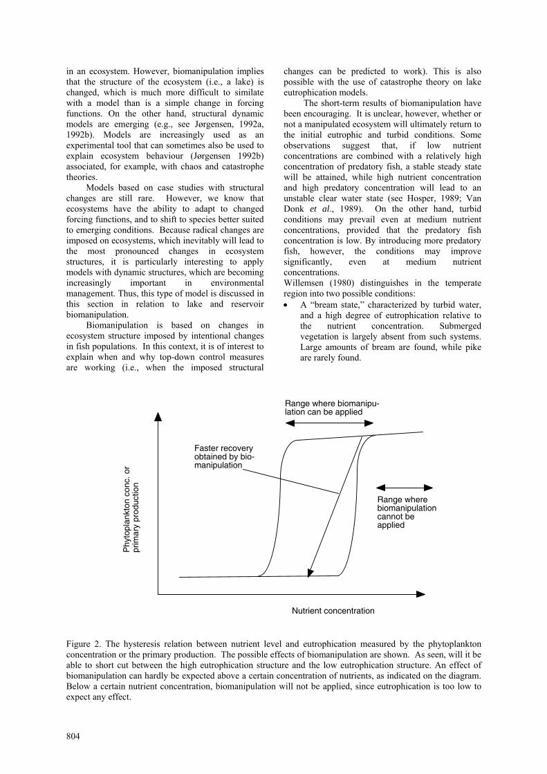
Figure 2. The hysteresis relation between nutrient level and eutrophication measured by the phytoplankton concentration or the primary production. The possible effects of biomanipulation are shown. As seen, will it be able to short cut between the high eutrophication structure and the low eutrophication structure. An effect of biomanipulation can hardly be expected above a certain concentration of nutrients, as indicated on the diagram. Below a certain nutrient concentration, biomanipulation will not be applied, since eutrophication is too low to expect any effect.

• A “pike state,” characterized by clear water, and

a low degree eutrophication relative to the nutrient level. Pike are abundant, while significantly fewer breams are found, compared with the "bream state." Willemsen's work shows that the pike/bream ratio is strongly correlated with water transparency and that the separation between the two states is relatively distinct. This behaviour is clearly analogous to other

examples described by catastrophe theory applied to biological systems (Jørgensen 1992a, 2002). The discontinuous response to increasing and decreasing nutrient levels implies that decreased nutrient levels will not cause a significant decrease in lake or reservoir eutrophication, and a significant increase in water transparency, before a rather low level has been attained. It may be possible, however, to "push" the equilibrium from point 3 to point 1 with the addition of predatory fish. This modelling example illustrates that two different concentrations of planktivorous fish can coexist with a certain nutrient concentration, which explains the hysteresis reaction shown in Figure 2. The general modelling experience is that a given set of forcing functions will give a certain set of state variables, including the concentration of planktivorous fish. However, when the set of equations that describe the ecosystem has a formulation causing catastrophic behavior in the mathematical sense, the reactions described above are observed.

To further explain these observations, models have been used as an experimental tool in the sense that the model description is in accordance with well-working lake models, but for which simulations with forcing functions for which there are no data available to control the model output, are carried out. Only phosphorus is considered as a nutrient in this case, although it is feasible to consider both nitrogen and phosphorus. The model encompasses the entire food chain. The modelling problem in the case of different inputs of nutrients, however, is that the phytoplankton, zooplankton, planktivorous and carnivorous fish are all able to adjust their growth rates within certain ranges. Thus, it is necessary to test a series of simulations with different combinations of growth rates to find which combination can give the highest probability of survival for all four classes of species. The results of these simulations can be summarized in the following points: • Between a total phosphorus (TP) concentration

of 70 – 130 μg/L, two levels of planktivorous fish give a stable situation, with a high probability of survival for all four classes of species. The level with the lowest level of planktivorous fish give the highest concentration of zooplankton and carnivorous fish, while the phytoplankton concentration is lowest. This interval from 70 -130 μg/L is, of course,

dependent on the model descriptions of the lake and must not be taken as fixed values for all lakes. Rather, they only indicate that there is an interval corresponding approximately to mesotrophic conditions are approximately two stable situations.

• The stable situation with the lowest level of planktivorous fish corresponds to the lowest growth rate of zooplankton and phytoplankton, which normally implies species that are larger in size (see Peters, 1983).

• Only one stable level is achieved at total phosphorus concentrations below 70 μg/L or above 130 μg/L. The zooplankton, relative to the level of phytoplankton, are present in highest levels at total phosphorus concentrations below 70 μg/L and relatively low above 130 μg/L.

• When the planktivorous fish are present at low concentrations either below total phosphorus concentrations of 70 μg/L, or between 70 – 130 μg/L, the phytoplankton is controlled by the relatively high zooplankton level (i.e., the grazing pressure), while phytoplankton at a high planktivorous level above total phosphorus concentrations above 70 μg/L is controlled by the nutrient concentration. As already underlined, this exercise should only

be considered qualitatively. However, the results suggest that the use of biomanipulation seems only to be successful at an intermediate nutrient level, which is consistent with the results of many biomanipulation experiments. The range at which biomanipulation can be used successfully is most probably dependent on the specific conditions in the considered lakes, which unfortunately makes it problematic to use results described in this section more qualitatively. The model example here uses a test of many combinations of growth rates to find the best combination of parameters from a survival perspective. This adjustment of the parameters corresponds to adaptation within some ranges, and for more radical changes of the parameters to a change in the species composition in the lake. If models are to be used as management tool in cases where significant changes in nutrient levels will occur, or where biomanipulation is being considered, it is necessary to develop models that can account for structural dynamic changes. However, this model development is still in its infancy. Thus, only limited experience is available.

Our present models have generally rigid structures and a fixed set of parameters, indicating that no changes or replacements of the components are possible. However, it is necessary to introduce parameters (properties) that can change according to changing general conditions for the state variables (components). The current idea is to test if a change of the most crucial parameters produces a higher so-

805

called goal function of the system and, if so, to use that set of parameters.

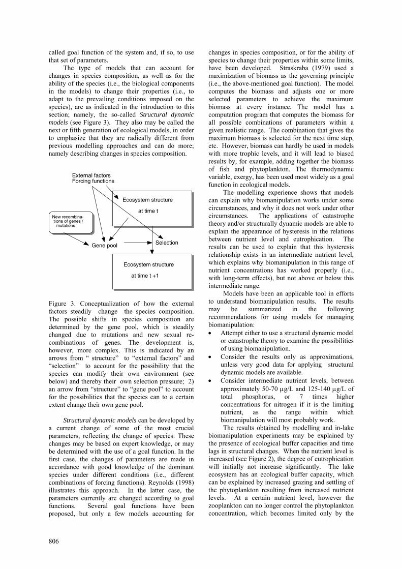
The type of models that can account for changes in species composition, as well as for the ability of the species (i.e., the biological components in the models) to change their properties (i.e., to adapt to the prevailing conditions imposed on the species), are as indicated in the introduction to this section; namely, the so-called Structural dynamic models (see Figure 3). They also may be called the next or fifth generation of ecological models, in order to emphasize that they are radically different from previous modelling approaches and can do more; namely describing changes in species composition.

External factors Forcing functions

Ecosystem structure at time t

Ecosystem structure at time t +1

New recombina- tions of genes / mutations

Gene pool Selection

Figure 3. Conceptualization of how the external factors steadily change the species composition. The possible shifts in species composition are determined by the gene pool, which is steadily changed due to mutations and new sexual re-combinations of genes. The development is, however, more complex. This is indicated by an arrows from “ structure” to “external factors” and “selection” to account for the possibility that the species can modify their own environment (see below) and thereby their own selection pressure; 2) an arrow from “structure” to “gene pool” to account for the possibilities that the species can to a certain extent change their own gene pool.

Structural dynamic models can be developed by a current change of some of the most crucial parameters, reflecting the change of species. These changes may be based on expert knowledge, or may be determined with the use of a goal function. In the first case, the changes of parameters are made in accordance with good knowledge of the dominant species under different conditions (i.e., different combinations of forcing functions). Reynolds (1998) illustrates this approach. In the latter case, the parameters currently are changed according to goal functions. Several goal functions have been proposed, but only a few models accounting for

changes in species composition, or for the ability of species to change their properties within some limits, have been developed. Straskraba (1979) used a maximization of biomass as the governing principle (i.e., the above-mentioned goal function). The model computes the biomass and adjusts one or more selected parameters to achieve the maximum biomass at every instance. The model has a computation program that computes the biomass for all possible combinations of parameters within a given realistic range. The combination that gives the maximum biomass is selected for the next time step, etc. However, biomass can hardly be used in models with more trophic levels, and it will lead to biased results by, for example, adding together the biomass of fish and phytoplankton. The thermodynamic variable, exergy, has been used most widely as a goal function in ecological models.

The modelling experience shows that models can explain why biomanipulation works under some circumstances, and why it does not work under other circumstances. The applications of catastrophe theory and/or structurally dynamic models are able to explain the appearance of hysteresis in the relations between nutrient level and eutrophication. The results can be used to explain that this hysteresis relationship exists in an intermediate nutrient level, which explains why biomanipulation in this range of nutrient concentrations has worked properly (i.e., with long-term effects), but not above or below this intermediate range.

Models have been an applicable tool in efforts to understand biomanipulation results. The results may be summarized in the following recommendations for using models for managing biomanipulation: • Attempt either to use a structural dynamic model

or catastrophe theory to examine the possibilities of using biomanipulation.

• Consider the results only as approximations, unless very good data for applying structural dynamic models are available.

• Consider intermediate nutrient levels, between approximately 50-70 μg/L and 125-140 μg/L of total phosphorus, or 7 times higher concentrations for nitrogen if it is the limiting nutrient, as the range within which biomanipulation will most probably work. The results obtained by modelling and in-lake

biomanipulation experiments may be explained by the presence of ecological buffer capacities and time lags in structural changes. When the nutrient level is increased (see Figure 2), the degree of eutrophication will initially not increase significantly. The lake ecosystem has an ecological buffer capacity, which can be explained by increased grazing and settling of the phytoplankton resulting from increased nutrient levels. At a certain nutrient level, however the zooplankton can no longer control the phytoplankton concentration, which becomes limited only by the

806

nutrient level. The result is that the eutrophication level increases considerably with increased nutrient levels. The entire structure of the ecosystem is changed because phytoplankton is now limited by nutrients, zooplankton by the predation from planktivorous fish rather than by the available food source (phytoplankton), and the planktivorous fish are now limited by the food source (zooplankton) rather than by the carnivorous fish.

This implies that other properties are selected (e.g., other growth rates). Further, the carnivorous fish will be scarce since they mostly hunt by sight, with the increasing eutrophication causing an increased turbidity and, therefore, making hunting more difficult.

If nutrient levels are now decreased by, for example, discharging wastewater with significantly lower nutrient concentrations, will this “high eutrophication structure,” characterized with a low concentration of carnivorous fish, high concentration of planktivorous fish, low concentration of zooplankton, and high concentration of phytoplankton, change immediately?

Thus, the low transparency will still make an increase in the carnivorous fish difficult, and grazing will still not able to control the phytoplankton concentration. This is because they are present in relatively low concentrations, since they are still under stress from considerable predation pressure by planktivorous fish. In this situation, will biomanipulation either by removal of planktivorous fish and/or introduction of more carnivorous fish, give a clear effect, as shown in Figure 2. Biomanipulation simply provides a faster recovery to the “low eutrophication structure,” where grazing controls the phytoplankton concentration. Outside the intermediate nutrient level, the forcing functions (input of nutrients) determine the state of eutrophication.

Models are a useful tool for trying to understand the function of biomanipulation, including the fact that it sometimes gives positive results, sometimes negative results. Models generally should be used as a tool to try to qualitatively understand the behavior of complex systems (e.g., lake ecosystems). When a good data base is available, models can sometimes be used quantitatively in environmental management, an example being the control of eutrophication by wastewater management (e.g., see Jørgensen and Vollenweider, 1988; Jørgensen, 1986, and Jørgensen et al., 2002). The use of models in a quantitative sense for biomanipulation efforts is possible by applying structural dynamic models. However, because our experience with this latter type of models is limited, the modelling results should not be the sole management decision criteria, although the results may be used in a qualitative way. Thus, there is a clear need for the use of models in management and selection of biomanipulation techniques to try to

answer such questions as: Can biomanipulation give the desired results? How many planktivorous fish must be removed and/or how many carnivorous fish must be added? How many times, and with which frequency, should biomanipulation be used to ensure the anticipated results? Such questions can only rarely be answered today with the use of models, primarily because the data requirements would be too great for most case studies. Thus, it is recommended that more case studies on the use of models under such conditions be developed and supported with good data sets. Only with increased experience in using models for biomanipulation purposes can the urgently needed management tools be developed. General Application of Structurally Dynamic Models Our present models are built on generally-rigid structures, and a fixed set of parameters. No change or replacement of components is usually possible. However, we also need to introduce parameters (properties) which can vary according to changing general conditions for the state variables (components). The idea currently is to test whether a change of the most crucial parameters produces a higher so-called goal function of the system and, if so, to use that set of parameters.

As indicated in the introduction to this section, models that can account for change in species composition, and for the ability of the species (i.e., the biological components of the models) to change their properties (i.e., to adapt to the prevailing conditions imposed on them), are called structural dynamic models. They also may be called the next or fifth generation of ecological models, in order to underline that they are radically different from previous modelling approaches and can do more, including describing changes in species composition.

It could be argued that the ability of ecosystems to replace current species with others that are better adapted to the ecosystem, can be addressed by constructing models which incorporate all possible species for the entire study period. However, there are two essential disadvantages. First, such models become very complex, since they will contain many state variables for each trophic level. Thus, many more of them need to be calibrated and validated, which will introduce a high uncertainty, and render application of the model very case-specific (Nielsen 1992a, 1992b). In addition, the model will still be rigid and not replicate the ecosystem property of parameters that are continuously changing without changing species composition (Fontaine, 1981).

Several goal functions have been proposed, but only a few models have been developed that can account for change in species composition, or for the ability of the species to change their properties within some limits. Straskraba (1979) used maximisation of biomass as the governing principle

807

(the goal function). The model adjusts one or more selected parameters, in order to achieve maximum biomass at every instance. A modeling software routine is included which computes biomass for all possible combinations of parameters within a given realistic range. The combination that gives the maximum biomass is selected for the next time step, etc. However, the biomass can hardly be used in models with more trophic levels. To add the biomass of fish and phytoplankton together, for example, will lead to biased results.

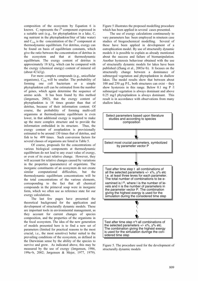
The thermodynamic variable, exergy, has been used most widely as a goal function in ecological models. One of the few lake case studies available is discussed below. There are two pronounced advantages of exergy as a goal function, compared to entropy and maximum power (Odum, 1983). These are that (1) it is defined far from thermodynamic equilibrium, and (2) it is related to state variables which are easily determined or measured. However, because exergy is not a common thermodynamic function, we need first to describe it.

Exergy expresses energy with a built-in measure of quality, quantifies natural resources, and can be considered as fuel for any system that converts energy and matter in a metabolic process (Schrödinger, 1944). Thus, ecosystems convert exergy, and exergy-flow through the system is necessary to keep it functioning. Exergy (as the amount of work the system can perform when brought into equilibrium with its environment) measures the distance from the “inorganic soup” in energy terms, as will be explained further below. Thus, exergy is dependent both on the environment and the system, rather than the system alone. This means, for example, that it is not a state variable like free energy and entropy.

Ecosystem at temperature T and pressure p

Reference system: the same system at the same temperature and pressure but at thermody- mic equilibrium

WORK CAPACITY = ECO-EXERGY = i=n Σ mi ( µi - µio) i=0

where mi is the amount of compo- nent i and µi is the chemical poten- tial of component i in the ecosystem µio is the corresponding chemical potential at thermodynamic equili- brium

Figure 4. Definition the applied concept, exergy or eco-exergy, in structurally dynamic modelling.

If we assume a reference environment representing an ecosystem at thermodynamic equilibrium, the configuration illustrated in Figure 4 is valid. All components are inorganic, at the highest possible oxidation state, and homogeneously distributed in the system. Thus, as much free energy as possible is utilized to perform work (no gradients). As the chemical energy embodied in the organic components and the biological structure contributes the most by far to the exergy content of the system, there seems to be no reason to assume a (minor) temperature and pressure difference between it and the reference environment. Under these circumstances, we can calculate the exergy content of the system provided entirely by chemical energy: Σc (µc - µceq) Ni. We can also determine its exergy, compared with that of a similar system at the same temperature and pressure, but in the form of an inorganic soup without any life, biological structure, informational or organic molecules. Because (µc - µceq) can be found from the definition of the chemical potential (replacing activities by concentrations), the following expressions for the exergy can be obtained:

i=n Ex = RT ΣCi ln Ci / Ci,eq (6) i=0 As seen, exergy measures the difference

between free energy (given the same temperature and pressure) of an ecosystem, and that of the surrounding environment. If the system is in equilibrium with its surroundings, exergy is zero, with n = 0 accounting for inorganic compounds, and n = 1 corresponding to detritus.

Since the only way to shift systems away from equilibrium is to perform work on them, and since the available work in a system is a measure of its ability to do so, we need to distinguish between the system and its environment (or thermodynamic equilibrium alias the inorganic soup). Thus, it is reasonable to use the available work (i.e., the exergy) as a measure of the distance from thermodynamic equilibrium.

Survival implies the maintenance of biomass, while growth means its increase. Exergy is needed to construct biomass, which then possesses exergy transferable to support other processes. Thus, survival and growth can be measured by use of the thermodynamic concept exergy, which may be understood as the free energy relative to the environment.

Darwin`s theory of natural selection, therefore, may be reformulated in thermodynamic terms and expanded to an ecosystem level as follows: The prevailing conditions of an ecosystem steadily change. The system will continuously select those species which contribute most to the maintenance, or even to the growth of the exergy of that system.

It is not possible to measure exergy directly. However, it is possible to compute it, if the

808

composition of the ecosystem by Equation 6 is known. Ci represents the ith component expressed in a suitable unit (e.g., for phytoplankton in a lake, Ci mg nutrient in the phytoplankton/liter of lake water) and Ci,eq is the concentration of the ith component at thermodynamic equilibrium. For detritus, exergy can be found on basis of equilibrium constants, which give the ratio between the concentration of detritus in the ecosystem and that at thermodynamic equilibrium. The exergy content of detritus is approximately 18 kJ/g, which can be compared with the exergy (chemical energy) content of mineral oil (about 42 kJ/g).

For more complex compounds (e.g., unicellular organisms), Ci,eq will be smaller. The probability of forming one coli bacterium or a simple phytoplankton cell can be estimated from the number of genes, which again determine the sequence of amino acids. It has been found by this method (Jørgensen, 2002), that the exergy content of phytoplankton is 18 times greater than that of detritus, because of their information content. Of course, the probability of forming multi-cell organisms at thermodynamic equilibrium is even lower, in that additional exergy is required to make up the more complex structure and to provide the information embedded in its structure. Thus, the exergy content of zooplankton is provisionally estimated to be around 130 times that of detritus, and fish to be 499 times. Such conversion factors for several classes of organisms are listed in Table 5.

Of course, proposals for the concentrations of various biological components at thermodynamic equilibrium do not lead to any exact value of exergy, or even of its exact relative change. However, they will account for relative changes caused by variations in the properties (parameters) of organisms. The inorganic constituents of an ecosystem do not create similar computational difficulties, but the thermodynamic equilibrium concentrations will be the total concentrations of the various elements, corresponding to the fact that all chemical compounds in the primeval soup were in inorganic form, which we often use as reference state for our exergy calculations.

The last few pages have presented the theoretical background for the application and development of structurally dynamic models. These are important tools in environmental management, as they account for current changes of species composition, and the properties of the organisms in the focal ecosystem. The idea of the new generation of models presented here is to find a new set of parameters (limited for practical reasons to the most crucial, i.e., the most sensitive) better suited to the prevailing conditions of the ecosystem, as defined in the Darwinian sense by the ability of the species to survive and grow. As indicated above, this may be measured by the use of exergy (Jørgensen, 1986, 199a+b, 2002; Jørgensen & Mejer, 1977, 1979).

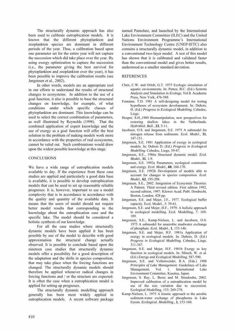
Figure 5 illustrates the proposed modelling procedure which has been applied in several cases presented.

The use of exergy calculations continuously to vary parameters has been employed in nineteen case studies of biogeochemical modelling. Several of these have been applied in development of a eutrophication model. By use of structurally dynamic models it is possible to explain as already mentioned about the success and failure of biomanipulation. Another hysteresis behaviour obtained with the use of structurally dynamic models for lakes have been published (Zhang et al., 2003a+b). It focuses on the structurally change between a dominance of submerged vegetation and phytoplankton in shallow lakes. The model results show that between about 100 and 250 µg P/L, both structures can exist – they show hysteresis in this range. Below 0.1 mg P /l submerged vegetation is always dominant and above 0.25 mg/l phytoplankton is always dominant. This result is in accordance with observations from many shallow lakes.

Select parameters based upon ltierature studies and according to species composition

Select most crucial parameters, symbolized by parameter vector P

Test after time step t all combinations of all the selected parameters +/- x%, y% etc i.e. at least three leves for each parameter. The total number of combinations to be e- xamined is l n, where l is the number of le- vels and n is the number of parameters in the parameter vector P. The combination giving the highest exergy is used for the simulation during the considered time step

Test after time step n*t all combinations of the selected parameters +/- x%, y% etc. The combination giving the highest exergy is used for the simulation duringe the con- sidered time step

Figure 5. The procedure used for the development of structurally dynamic models

809

The structurally dynamic approach has also been used to calibrate eutrophication models. It is known that the different phytoplankton and zooplankton species are dominant in different periods of the year. Thus, a calibration based upon one parameter set for the entire year will not capture the succession which did take place over the year. By using exergy optimization to capture the succession (i.e., the parameter giving the best survival for phytoplankton and zooplankton over the year), it has been possible to improve the calibration results (see Jørgensen et al., 2002).

In other words, models are an appropriate tool in our efforts to understand the results of structural changes to ecosystems. In addition to the use of a goal function, it also is possible to base the structural changes on knowledge, for example, of what conditions under which specific classes of phytoplankton are dominant. This knowledge can be used to select the correct combination of parameters, as well illustrated by Reynolds (1998). That the combined application of expert knowledge and the use of exergy as a goal function will offer the best solution to the problem of making models work more in accordance with the properties of real ecosystems, cannot be ruled out. Such combinations would draw upon the widest possible knowledge at this stage. CONCLUSIONS We have a wide range of eutrophication models available to day. If the experience from these case studies are applied and particularly a good data base is available, it is possible to develop eutrophication models that can be used to set up reasonable reliable prognoses. It is, however, important to use a model complexity that is in accordance in accordance with the quality and quantity of the available data. It means that the users of model should not require better model results that corresponding to the knowledge about the eutrophication case and the specific lake. The model should be considered a holistic synthesis of our knowledge.

For all the case studies where structurally dynamic models have been applied it has been possible by use of the model to describe with good approximation the structural change actually observed. It is possible to conclude based upon the nineteen case studies that structurally dynamic models offer a possibility for a good description of the adaptation and the shifts in species composition, that may take place when the forcing functions are changed. The structurally dynamic models should therefore be applied whenever radical changes in forcing functions and / or the structure are expected. It is often the case when a eutrophication model is applied for setting up prognoses.

The structurally dynamic modelling approach generally has been most widely applied in eutrophication models. A recent software package

named Pamolare, and launched by the International Lake Environment Committee (ILEC) and the United Nations Environment Programme’s International Environment Technology Centre (UNEP-IETC) also contains a structurally dynamic model, in addition to a conventional two-layer model. A test of this model has shown that it is calibrated and validated faster than the conventional model and gives better results, understood as a smaller standard deviation. REFERENCES Chen, C.W. and Orlob, G.T. 1975 Ecologic simulation of

aquatic environments. In: Patten, B.C. (Ed.) Systems Analysis and Simulation in Ecology, Vol.3. Academic Press, New York, 476-588.

Fontaine, T.D. 1981 A self-designing model for testing hypotheses of ecosystem development. In: Dubois, D. (Ed.) Progress in Ecological Modelling. Cebedoc, Liege.

Hosper, S.H.,1989 Biomanipulation, new perspectives for restoring shallow lakes in the Netherlands. Hydrobiol. Bull., 23, 5-11.

Jacobsen, O.S. and Jørgensen, S.E. 1975 A submodel for nitrogen release from sediments. Ecol. Model., 31, 147-151.

Jørgensen, S.E. 1981 Application of exergy in ecological models. In: Dubois D. (Ed.) Progress in Ecological Modelling. Cebedoc, Liege, 39-47.

Jørgensen, S.E., 1986a Structural dynamic model. Ecol. Model., 31, 1-9.

Jørgensen, S.E. 1992a Parameters, ecological constraints and exergy. Ecol. Model., 60, 160-170.

Jørgensen, S.E. 1992b Development of models able to account for changes in species composition. Ecol. Model., 62, 195-208.

Jørgensen, S.E., 2002. Integration of Ecosystem Theories: A Pattern. Third revised edition. First edition 1992, second edition, 1997. Kluwer Acad. Publ. Dordrecht, Boston, London. 428 pp.

Jørgensen, S.E. and Mejer, J.F., 1977. Ecological buffer capacity. Ecol. Model., 3: 39-61.

Jørgensen, S.E. and Mejer, H.F., 1979. A holistic approach to ecological modelling. Ecol. Modelling, 7: 169-189.

Jørgensen, S.E., Kamp-Nielsen, L. and Jacobsen, O.S. 1975 A submodel for anaerobic mudwater exchange of phosphate. Ecol. Model., 1, 133-146.

Jørgensen, S.E. and Mejer, H.F. 1981a Application of exergy in ecological models. In: Dubois, D. (Ed.) Progress in Ecological Modelling. Cebedec, Liege, 311-347.

Jørgensen, S.E. and Mejer, H.F. 1981b Exergy as key function in ecological models. In: Mitsch, W. et al. (Ed.) Energy and Ecological Modelling, 587-590.

Jørgensen, S.E. and Vollenweider, R.A. (Eds.) 1988 Principles of Lake Management. Guidelines of Lake Management, Vol. 1. International Lake Environment Committee, Kusatsu, Japan.

Jørgensen, S. Ray, L. Berec and M. Straskraba, 2002. Improved calibration of a eutrophication model by use of the size variation due to succession. Ecological Modelling, 153: 269-278.

Kamp-Nielsen, L. 1975 A kinetic approach to the aerobic sediment-water exchange of phosphorus in Lake Esrom. Ecological. Modelling., 1, 153-160.

810

811

Nielsen, S.N. 1992a Application of Maximum Energy in Structural Dynamic Models. Ph.D. Thesis. National Environmental Research Institute. Denmark.

Nielsen, S.N. 1992b Strategies for structural-dynamic modelling. Ecological. Modelling., 63, 91-100.

Odum, H.T. 1983. System Ecology. Wiley Interscience, New York. 510 pp.

OECD (Organization for Economic Cooperation and Development). Eutrophicatoin Study (get complete reference).

Peters, R.H. 1983 The Ecological Implications of Body Size. Cambridge Univ. Press, Cambridge.

Rast, W. and Thornton, J.A. 1996. Trends in eutrophication research and control. Hydrological Processes., 10(2), 295-313.

Reynolds, C.S. 1998 What factors influence the species composition of phytoplankton in lakes of different trophic status? Hydrobiologia., 369/370, 11-26

Schrödinger, E., 1944. What is life? Cambridge University Press. 212 pp.

Straskraba, M. 1979 Natural control mechanisms in models of aquatic ecosystems. Ecol. Model., 6, 305-322.

Van Donk, E., Gulati, R.D. and Grimm, M.P. 1989 Food web manipulation in Lake Zwemlust: positive and negative effects during the first two years. Hydrobiol. Bull., 23, 19-35.

Willemsen, J. 1980 Fishery aspects of eutrophication. Hydrobiol. Bull., 14, 12-21.

WMO 1975 Intercomparison of Conceptual Models used in Operational Hydrological Forecasting. Geneva.

Zhang, J., Jřrgensen, S.E., Tan C.O., Beklioglu, M., 2003a. A structurally dynamic modelling - Lake Mogan, Turkey as a case study. Ecological Modelling 164, 103-120.

Zhang, J., Jřrgensen, S.E., Tan C.O., Beklioglu, M., 2003b. Hysteresis in vegetation shift - lake Mogan Prognoses. Ecological Modelling 164, 227-238.