Working Paper n° 15/06 Madrid, February 2015
Monitoring the world business cycle
Máximo Camacho
Jaime Martínez-Martín

1 / 2 www.bbvaresearch.com
15/06 Working Paper
February 2015
Monitoring the world business cycle*
Máximo Camacho1 and Jaime Martínez-Martín
2
Abstract
We propose a Markov-switching dynamic factor model to construct an index of global business cycle
conditions, to perform short-term forecasts of world GDP quarterly growth in real time and to compute real-
time business cycle probabilities. To overcome the real-time forecasting challenges, the model accounts for
mixed frequencies, for asynchronous data publication and for leading indicators. Our pseudo real time
results show that this approach provides reliable and timely inferences of the world quarterly growth and of
the world state of the business cycle on a monthly basis.
Keywords: Real-time forecasting, world economic indicators, business cycles,non-linear dynamic factor
models.
JEL: E32, C22, E27.
* We would like to thank J.J. Cubero, M. Martinez-Alvarez and seminar participants at the Bank of Spain and BBVA Research for their helpful comments. M. Camacho thanks CICYT for its support through grant ECO2013-45698. Part of this research was developed when J. Martinez-Martin was working for BBVA Research. All the remaining errors are our own responsibility. The views in this paper are those of the authors and do not represent the view of the Bank of Spain or the Eurosystem. No part of our compensations were, are or will be directly or indirectly related to the specific views expressed in this paper. Corresponding author: Jaime Martinez-Martin, Bank of Spain, Alcalá 48, 28014, Madrid, Spain E-mail: [email protected] 1: U Murcia & BBVA Research; [email protected] 2: Bank of Spain; [email protected]

1 Introduction
The drastic downturn in the global economy in 2009 led the economic agents to acknowl-
edge the need for new tools to monitor the ongoing world economic developments, which
may especially affect small open economies. Although there is currently no global statis-
tical institute in charge of providing offi cial quarterly national accounts at a global level,
the IMF releases real GDP annual growth rate figures on an annual basis. However, the
IMF only releases its GDP figures twice a year (usually in April and October), although
there are two additional updates in January and July, but these provide much less detail.
Therefore, the target of the recent literature has been focusing on several indicators at
higher frequencies, which are promptly available and are used to construct early estimates
of the world GDP. Rossiter (2010) uses bridge equations to show that PMIs are useful for
forecasting developments in the global growth. Within the bridge equation framework,
Golinelli and Parigi (2014) detect that short-run indicators from advanced and emerging
countries help in predicting the world variables and Drechsel et al. (2014) find that several
monthly leading global indicators improve upon the world forecasts of the IMF. Ferrara
and Marsilli (2014) develop a linear Dynamic Factor Model (DFM) to summarise the
information of a large monthly database into a small numbers of factors and use the
MIDAS framework to show that they improve upon the IMF forecasts, at least at the
beginning of each year.
These approaches suffer from two limitations. The first limitation is that they focus
on GDP on an annual basis while the IMF also releases GDP quarterly growth rates
sampled on a quarterly basis. In spite of the advantage in managing data on a quarterly
basis, the IMF releases its quarterly figures sporadically, with long publication delays (9
months on average) and no fixed starting date. Hence, to the best of our knowledge, its
longest available world GDP quarterly series begins in 2007, which clearly restricts the
econometric analysis. To overcome this drawback, we reproduce the IMF releases of the
world GDP on a quarterly basis by following the same methodology. Both series are the
same from 2007 up to the present, but our series dates back to 1991.
The second limitation of these approaches is that they all rely on linear specifications,
2

which handicaps the models in capturing the nonlinearities that characterise the world
business cycle fluctuations and can be used for detecting turning points. To overcome this
drawback, we propose an extension of the Markov-switching DFM (MS-DFM) suggested
in Camacho et al. (2012). As in their proposal, the MS-DFM advocated by Kim and
Yoo (1995), Chauvet (1998) and Kim and Nelson (1998) is enabled to deal with mixing
frequencies, publication delays and different starting dates in the economic indicators.
In this framework, low-frequency indicators are treated as high-frequency indicators with
missing observations and the model is estimated by using a time-varying nonlinear Kalman
filter. In addition, we extend the model to handle leading indicators, which are very useful
in short-term forecasting (Camacho and Martinez-Martin, 2014) since they usually start
to decline before the economy as a whole declines, and start to improve before the general
economy begins to recover from a slump. We allow the data to select the number of periods
by which the leading indicators lead the broad economic activity, from a minimum of one
quarter to one and a half years.
In the empirical application, we use this extension to evaluate the accuracy of the model
in computing short-term forecasts of world GDP, and to reveal inferences about the state
of the global economy from six economic indicators: the quarterly world GDP and the
monthly global industrial production index, the global manufacturing Purchasing Manager
Index (PMI), the employment index, the new export orders index and the CBOE volatility
index (VIX). For this purpose, we develop a pseudo real-time forecasting exercise, where
data vintages are constructed from successive enlargements of the latest available data set
by taking into account the real-time data flow (and hence the publication lags). Therefore,
the experiment tries to mimic as closely as possible the real-time analysis that would have
been performed by a potential user of the models when forecasting, in each period, on the
basis of different vintages of data sets. In line with the substantial publication delay of
world GDP, in each forecast period we perform backcasts (predict the previous quarters
before data for those quarters are released) nowcasts (predict the current period) and
forecasts (predict the next quarter).
Our main results are as follows. First, the percentage of the variance of world GDP
growth that is explained by our MS-DFM is slightly above 70%, indicating the high poten-
3

tial ability of our extension to explain global growth. Second, our pseudo real-time analysis
shows that our MS-DFM clearly outperforms univariate forecasts, especially when back-
casting and nowcasting. In addition, our MS-DFM also outperforms the forecasts of a
linear DFM. Third, our business cycle indicator is in striking accord with the consensus of
the history of the world business cycle (Grossman et al. 2014). Fourth, we also compare
the performance of the fully non-linear MS-DFM (one-step approach) with the “shortcut”
of using a linear DFM to obtain a coincident indicator which is then used to compute the
Markov-switching probabilities (two-step approach). In line with Camacho et al. (2015),
our results suggest that the one-step approach is preferred to the two-step approach to
compute inferences on the business cycle phases.
The structure of this paper is organised as follows. Section 2 describes the method-
ological considerations of the model. Section 3 contains data descriptions and the main
empirical results. Section 4 concludes.
2 The econometric model
To account for the peculiar characteristics of the data flow in real time, the comovements
across the economic indicators and the business cycles asymmetries, we start from the
approach suggested in Camacho et al. (2012). This model is extended to handle economic
indicators that lead the broad economic activity.
2.1 Mixing frequencies
The approach deals with the problem of mixing monthly and quarterly frequencies of
flow data by treating quarterly series as monthly series with missing observations. Let us
assume that the levels of the quarterly flow variable in the quarter that ends in month t,
Gt, can be decomposed as the sum of three unobservable monthly values Xt, Xt−1, Xt−2,
where t, t− 1 and t− 2 refer to the three months of that quarter
Gt = 3Xt +Xt−1 +Xt−2
3. (1)
Following the linear framework described in Mariano and Murasawa (2003), let us assume
that the arithmetic means can be approximated by geometric means. Hence, the level of
4

the quarterly flow variable becomes
Gt = 3(XtXt−1Xt−2)1/3. (2)
Applying logs and taking the three-period differences for all t
43 lnGt =1
3(43 lnXt +43 lnXt−1 +43 lnXt−2). (3)
Calling 43 lnGt = gt, and 4 lnXt = xt, and after a little algebra
gt =1
3xt +
2
3xt−1 + xt−2 +
2
3xt−3 +
1
3xt−4, (4)
which shows that that quarterly growth rates of the quarterly flow variable can be viewed
as sums of underlying monthly growth rates of the underlying monthly series.
2.2 Dynamic properties
Let us assume that the n indicators included in the model, yit , i = 1., ..., n, admit a
dynamic factor representation. In this case, the indicators can be written as the sum of
two stochastic components: a common component, ft, which represents the overall busi-
ness cycle conditions, and an idiosyncratic component, uit, which refers to the particular
dynamics of the series.
To account for the business cycle asymmetries, we assume that the underlying business
cycle conditions evolve with AR(pf ) dynamics, which is governed by an unobserved regime-
switching state variable, st,
ft = cst + θ1ft−1 + ...+ θpf ft−p + εft, (5)
where εft˜iN(
0, σ2f
). Within this framework, one can label st = 0 and st = 1 as the
expansion and recession states at time t. In addition, it is standard to assume that the
state variable evolves according to an irreducible 2-state Markov chain, whose transition
probabilities are defined by
p(st = j|st−1 = i, st−2 = h, ..., It−1) = p(st = j|st−1 = i) = pij (6)
where i, j = 0, 1 and It is the information set up to period t.
5

Coincident indicators, such as the monthly growth rates of GDP and the monthly
growth rates of industrial production index, the global manufacturing Purchasing Man-
ager Index (PMI) index, the employment index and the new export orders index depend
contemporaneously on ft and on their idiosyncratic dynamics, uit, which evolve as an
AR(pi)
yit = βift + uit, (7)
uit = θi1uit−1 + ...+ θipiut−pi + εit, (8)
where εit˜iN(0, σ2i
), i = 1, ..., 5. However, since leading indicators lead the economy
movements by h periods, VIX is assumed to depend on the h-period future values of the
common factor and its idiosyncratic dynamics, uit, which evolve as an AR(p6)
ylt = βlft+h + ult, (9)
ult = θl1ult−1 + ...+ θ6plut−pl + εlt, (10)
where εlt˜iN(0, σ2l
). Finally, we assume that all the shocks εft and εit, i = 1, ..., 6, are
mutually uncorrelated in cross-section and time-series dimensions.
2.3 State space and missing observations
Assuming that all variables are always observed at a monthly frequency, it is standard
to cast the model in state form. The state-space model represents a set of observed time
series, Yt, as linear combinations of a vector of auxiliary variables, which are collected on
the state vector, ht. This relation is modeled by the measurement equation, Yt = Hξt+Et,
with Et ∼ i.i.d.N (0, R). The Appendix provides more details on the model structure and
the specific forms of these matrices. The dynamics of the state vector are modelled by
the transition equation ht = Λst + Fht−1 + Vt, with Vt ∼ i.i.d.N (0, Q). Maximising the
exact log likelihood function of the associated nonlinear Kalman filter is computationally
burdensome since at each iteration the filter produces a 2-fold increase in the number of
cases to consider. The solution adopted in this paper is based on collapsing some terms
of the former filter as proposed by Kim (1994). In particular, our proposal is based on
collapsing the posteriors h(i,j)t|t and its covariance matrix P (i,j)t|t at the end of each iteration
6

by using their weighted averages for st = j, where the weights are given by the probabilities
of the Markov state
hjt|t
=
1∑st−1=0
p (st = j, st−1 = i|It)h(i,j)t|t
p (st = j|It)(11)
P jt|t
=
1∑st−1=0
p (st = j, st−1 = i|It)(P(i,j)t|t +
(hjt|t− h(i,j)t|t
)(hjt|t− h(i,j)t|t
)′)p (st = j|It)
. (12)
To handle missing data, we use the method used in Camacho et al. (2012). For this
purpose, we substitute missing observations with random draws θt from N(0, σ2θ). This
implies replacing the i-th row of Yt, Ht, Et (denoted by Yit, Hit and wit) and the i-th
element of the main diagonal of Rt (Riit), by Y ∗it , H∗it, E
∗it, and R
∗iit, respectively. The
starred expressions are Yit, Hit, 0, and 0 if the variable Yit is observable at time t, and
θt, 01,n, θt, and σ2θ in case of missing data. Accordingly, this transformation converts the
model in a time-varying state-space model with no missing observations and the nonlinear
version of the Kalman filter can be directly applied to Y ∗t , H∗t , w
∗t , and R
∗t since missing
observations are automatically skipped from the updating recursion.
To conclude this section, let us describe how our model can easily compute world GDP
growth forecasts. Let us assume that GDP growth is placed first Yt and let us call T the
last month for which we have observed this indicator and that we are interested in the
forecast for T + 1. Let us call h(j)T+1|T the collapsed version of h(i,j)T+1|T , and call h
(j)T+1|T (k)
the k-th element of h(j)T+1|T . Taking into account that ht contains ft +h and its lags, as
well as the idiosyncratic components and their lags, the forecasts for month T + 1 when
sT+1 = j can be computed from the model as
y(j)1T+1/T = β1
(1
3h(j)T+1|T (h+ 1) +
2
3h(j)T+1|T (h+ 2) + h
(j)T+1|T (h+ 3) +
2
3h(j)T+1|T (h+ 4) +
1
3h(j)T+1|T (h+ 5)
)+(
1
3h(j)T+1|T (h+ 6) +
2
3h(j)T+1|T (h+ 7) + h
(j)T+1|T (h+ 8) +
2
3h(j)T+1|T (h+ 9) +
1
3h(j)T+1|T (h+ 10)
).
(13)
Using the matrix of transition probabilities, one can easily obtain p (sT+1 = j, sT = i|It),
7

which can be used to compute
p (sT+1 = j|IT ) =2∑i=1
p (sT+1 = j, sT = i|IT ) (14)
Then, the unconditional forecast of GDP is
y1T+1/T =2∑j=1
p (sT+1 = j|χt) y(j)T+1/T . (15)
It is worth noting that these forecasts are easily computed in practice by including missing
observations of GDP growth in the dataset, since the model will automatically replace at
missing observation with a dynamic forecast. Following the same reasoning, forecasts for
longer horizons and forecasts for other indicators can be computed in this way.
3 Empirical results
3.1 Preliminary analysis of the data
In this section, we identify potential indicators that reflect the economic dynamics of the
world, and might therefore be well suited for the prediction of the GDP aggregates and
the business cycle conditions. Indicators should lead or coincide with the macroeconomic
dynamics of the particular aggregate, and should have a wide coverage of the economy as a
whole. In addition, they should have a high frequency, should be released before the GDP
figure for the respective quarter becomes available and must be available in at least one
third of the sample. For the world indicators, we have selected the following five coincident
indicators: the quarterly world GDP and the monthly global industrial production index,
the global manufacturing Purchasing Manager Index (PMI), the employment index and
the new export orders index. In addition, we include the CBOE volatility index (VIX),
which is a key measure of market expectations of near-term volatility conveyed by S&P
500 stock index option prices.
The data set managed in this paper was collected on 15 December, 2014 and the
maximum effective sample spans the period from January 1991 to October 2014. The
indicators used in the empirical analysis, their respective release lag-time, their sources
and the data transformations applied to achieve stationarity are listed in Table 1. GDP
8

enters the model as its quarterly growth rate, industrial production and the VIX enters in
monthly growth rates while other indicators enter with no transformation. All the variables
are seasonally adjusted. Before estimating the model, the variables are standardised to
have a zero mean and a variance equal to one. Therefore, the final forecasts are computed
by multiplying the initial forecasts of the model by the sample standard deviation, and
then adding the sample mean.1
[Insert Table 1 about here]
The IMF releases the quarterly data sporadically, with a long publication delay of
9 months on average. However, the most important limitation is that the historically
available series starts in 2007, which clearly restricts the econometric analysis. To overcome
this drawback, we aim to re-construct the IMF releases of the world GDP on a quarterly
basis by following the same methodology. Our proxy is based on the aggregation of national
quarterly growth rates (offi cial Quarterly National Accounts) of 69 countries, which are
weighted by their share of GDP ppp in the world.2 Both series are the same from 2007
up to the present but our world GDP quarterly growth is dated back to 1991.
3.2 In-sample analysis
We examine in this section the in-sample estimates of the nonlinear dynamic factor model
outlined in Section 2. For the contribution of this paper, the selection of the lead time
profile of the VIX becomes of particular interest, since it is allowed to lead the business
cycle dynamics in h months, with h = 0, 1, ..., 6. To select the optimal number of leads,
we computed the log likelihood values associated with these lead times and we observed
that the maximum of the likelihood function was achieved when the VIX led the common
factor by h = 3 months.
The loading factors, whose estimates appear in Table 2 (standard errors in paren-
theses), allow us to evaluate the correlation between the common factor and each of the
1 In the simulated real-time analysis, the sample means and standard deviations are also computed using
only the observations available up to the forecast jump-off point.2 It covers about 92% of total world GDP ppp.
9

indicators used in the model.3 Apart from GDP (loading factor of 0.22), the economic
indicators with the largest loading factors are industrial production (loading factor of
0.47) and the VIX (loading factor of -0.22). As expected, the loading factors for all of the
indicators except the VIX are positive and statistically significant, indicating that these
series are procyclical, i.e., positively correlated with the common factor that represents the
world overall economic activity. The significant negative sign of the VIX’s loading factor
agrees with the view that it becomes a leading proxy of global financial risk aversion.4 For
the sake of comparison, the table also shows the factor loadings of the linear version of
MS-DFM.
[Insert Table 2 about here]
Although GDP is generally regarded as the most appropriate indicator of economic
activity, global GDP is only available on an annual basis or, sporadically, a quarterly
basis. As such, many important questions cannot be addressed in a satisfactory manner,
especially those related to the analysis of business cycles. One partial solution is found
by constructing aggregate indexes at monthly frequency, which are computed as linear
combinations of meaningful economic indicators, as in Aruoba et al. (2011). However,
these indexes are not related to the particular variable of interest, what makes it diffi cult
to find an economic interpretation of their movements or their reactions to shocks. One
significant contribution of our methodology is that it allows to construct quarterly GDP
growth rates for the world economy on a monthly basis, from both available quarterly
GDP data and global monthly indicators. This time series is plotted in Figure 1.
[Insert Figure 1 about here]
Our model is based on the notion that co-movements among the macroeconomic vari-
ables have a common element, the common factor, that moves in accordance with the
dynamics of the world business cycle. To check whether the business cycle information
3The lag lengths used in the empirical exercise were always set to 2. However, we performed several
exercises to check that our results were robust to other reasonable choices of the lag lengths.4Under the framework of financial publications and business news’ shows on CNBC, Bloomberg TV
and CNN/Money, the VIX is often referred to as the “fear index”.
10

that can be extracted from the common factor agrees with the world business cycle, the
coincident indicator is also plotted in Figure 1.5 According to this figure, the evolution
of the factor is in clear concordance with GDP growth and contains relevant information
of its expansions and recessions. In particular, the common factor is consistent with the
recession of the early 1990s, the expansionary period of the late 1990s and the downturn
of 2001. The evolution of the factor also picks up the short-lived effects of the Asian
financial crisis of 1997 and the Russian default of 1998 as an emerging markets slowdown.
In addition, it also captures the magnitude of the global recession of 2008, which was
unprecedented in scale, and the subsequent (albeit fragile) recovery.
3.3 Pseudo real-time analysis
To begin with, it is worth mentioning that we could not perform the forecast evaluation
in pure real-time, i.e., by using only the information that would have been available at the
time of each forecast. The reason is that the historical records of the time series used in
the analysis were not available to construct all the real-time vintages for all the indicators
in the panel. One feasible alternative, employed frequently in the forecasting literature,
is to develop a pseudo real-time analysis. The method consists of computing forecasts
from successive enlargements of a partition of the latest available data set by taking into
account the typical real-time data flow when constructing the data vintages.6 Therefore,
the method tries to mimic as closely as possible the real-time analysis that would have
been performed by a potential user of the models when forecasting, at each time period.
Our pseudo real-time analysis begins with data of all the time series from the beginning
of the sample until October 2000. Since the average reporting lag of world GDP is three
quarters, we assume that the latest available figure of GDP refers to the first quarter
of 2000. Using this sample, the model is estimated and 15-months-ahead forecasts of
5To facilitate graphing, the coincident indicator has been transformed to exhibit the same mean and
variance as world GDP growth.6Hence, each vintage used at the forecast periods contains missing data at the end of the sample
reflecting the calendar of data releases. We assume that the pattern of data availability is unchanged
throughout the evaluation sample since the timing of data releases varies only slightly from month to
month.
11

quarterly GDP growth are computed. This implies performing backcasts for the first three
quarters of 2000, nowcasts for the last quarter of 2000 and forecasts for the first quarter of
2001. In addition, we collect the probabilities of recession for the first month of the quarter
for which GDP is unavailable. In November 2000, the sample is updated by one month of
each indicator, the model is reestimated and 15-months-ahead forecasts of quarterly GDP
growth and the inferences on the business cycle state for the second month of the quarter
for which GDP is unavailable are computed again. Then, the sample is again updated by
one month and the forecasting exercise is developed similarly in December 2000.
In January 2001, GDP for the first quarter of 2000 is assumed to be released so the
forecast moves forward one quarter. The forecasting procedure continues iteratively until
the final forecast with the last vintage of data that refers to July 2014, with the 15-months-
ahead forecasts moved forward one quarter in accordance with the publication date of
GDP. This procedure ends up with 165 blocks of forecasts. To examine the forecasting
accuracy, we compute the mean-squared forecast errors (MSE), which are the average of
the deviations of the predictions from the final releases of GDP available in the data set.
This paper establishes two naïve benchmark models against which to compare the
results of the MS-DFM model. The first benchmark is a random-walk model, where
the forecasts for the global output growth are equal to the last observed value. The
second benchmark model is an autoregressive model, in which GDP is regressed on its
lags and the forecasts are computed recursively from the in-sample estimates. Since these
types of models traditionally perform reasonably well with macro data, the key challenge
then is to determine whether the addition of global indicator variables can improve the
forecasting performance of the benchmark models. In addition, the paper also establishes
as a benchmark the linear dynamic factor model underlying the nonlinear specification. In
this case, the challenge is to determine whether accounting for the potential nonlinearities
help in improving the forecasting accuracy.
The predictive accuracy of the models is under examination in Table 3. Results for
backcasts, nowcasts and forecasts are summarised in the second, third and fourth columns,
respectively. Remarkably, the multivariate models perform better than the univariate
benchmarks, with largest improvements for shortest forecast horizons. This result rein-
12

forces the view that the monthly global indicators are useful for forecasting the develop-
ments in the global economy. When comparing MS-DFM and the linear DFM, the former
performs better than the latter. This suggests that to obtain accurate forecasts of world
GDP, the nonlinear information on the total economy matters.
[Insert Table 3 about here]
In spite of the good performance in forecasting world GDP, our nonlinear MS-DFM
exhibits a clear advantage with respect to the linear proposals. The model automatically
converts the economic information contained in the global indicators into inferences of the
world business cycle. In particular, the model computes probabilities of global recessions,
which are transparent, objective and free of units of measurement, facilitating business
cycle comparisons with national developments. Figure 2 plots the real-time probabili-
ties whenever the coincident global indicator is under a recessionary state. To facilitate
comparisons, the figure also shows shaded areas that refer to the chronology of global
recessions suggested in Grossman et al. (2014).7 Notably, they are in striking accord: the
probabilities of recession jump quickly around the peaks, remain at high values during
recessions and fall to almost zero after the troughs.
[Insert Figure 2 about here]
As a final check, we compare the performance of our fully nonlinear multivariate spec-
ification (one-step approach) with the ‘shortcut’of using a linear factor model to obtain
a coincident indicator, which is then used to compute the Markov switching probabilities
(two-step approach). We quantify the ability of these procedures to detect the actual state
of the business by computing the Forecasting Quadratic Probability Score (FQPS), i.e.,
the mean squared deviation of the probabilities of recessions from a recessionary indicator
that takes on the value of one in the periods classified by Grossman et al. (2014) as reces-
sions and zero elsewhere. We obtain a FQPS of 0.09 for the two-step approach, which falls
to 0.06 in the case of the one-step approach. Therefore, our results suggest that, in line7These authors date the turning points by using univariate dating algorithms to global aggregates of a
sample of 84 countries.
13

with Camacho et al. (2015), the one-step approach is preferred to the two-step approach
to compute inferences on the business cycle phases.
4 Concluding remarks
Albeit that several approaches have been employed, it has been a recent challenge to con-
struct practical and satisfactory tools to monitor global business cycles. The methodology
we use in this paper has several advantages over existing approaches. First, our measure
of global economic activity captures common movements among a wide range of indicators
that can exhibit different frequencies, different sample start dates and different release lags.
In particular, we include GDP, industrial production, manufacturing PMI, employment,
new export orders and VIX. Second, our framework is useful for computing short-term
forecasts of world GDP in real time. In addition, it combines the information provided
by monthly and quarterly data to obtain a monthly measure of quarterly growth rates
of world GDP. Managing data on a monthly basis has enormous advantages in several
macroeconomic applications, especially those related to business cycle analyses. Third,
our framework is also useful for monitoring global economic activity in real time. The
nonlinear nature of the model proposed in this paper helps it to capture the asymmet-
ric dynamics of the recurrent sequence of expansions and recessions that characterise the
world business cycle.
14
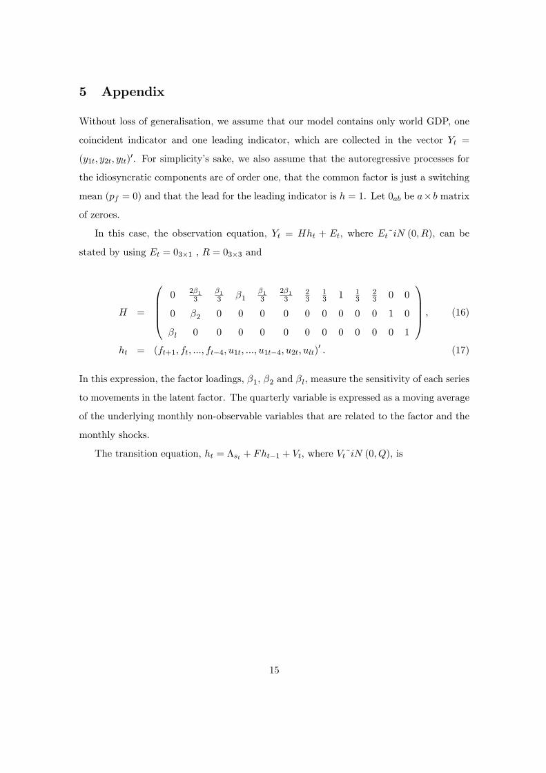
5 Appendix
Without loss of generalisation, we assume that our model contains only world GDP, one
coincident indicator and one leading indicator, which are collected in the vector Yt =
(y1t, y2t, ylt)′. For simplicity’s sake, we also assume that the autoregressive processes for
the idiosyncratic components are of order one, that the common factor is just a switching
mean (pf = 0) and that the lead for the leading indicator is h = 1. Let 0ab be a× b matrix
of zeroes.
In this case, the observation equation, Yt = Hht + Et, where Et˜iN (0, R), can be
stated by using Et = 03×1 , R = 03×3 and
H =
0 2β1
3β13 β1
β13
2β13
23
13 1 1
323 0 0
0 β2 0 0 0 0 0 0 0 0 0 1 0
βl 0 0 0 0 0 0 0 0 0 0 0 1
, (16)
ht = (ft+1, ft, ..., ft−4, u1t, ..., u1t−4, u2t, ult)′ . (17)
In this expression, the factor loadings, β1, β2 and βl, measure the sensitivity of each series
to movements in the latent factor. The quarterly variable is expressed as a moving average
of the underlying monthly non-observable variables that are related to the factor and the
monthly shocks.
The transition equation, ht = Λst + Fht−1 + Vt, where Vt˜iN (0, Q), is
15

Λst = (cst , 01×12)′ , (18)
F =
0 0 0 0 0 0 0 0 0 0 0 0 0
1 0 0 0 0 0 0 0 0 0 0 0 0
0 1 0 0 0 0 0 0 0 0 0 0 0
0 0 1 0 0 0 0 0 0 0 0 0 0
0 0 0 1 0 0 0 0 0 0 0 0 0
0 0 0 0 1 0 0 0 0 0 0 0 0
0 0 0 0 0 0 θ11 0 0 0 0 0 0
0 0 0 0 0 0 1 0 0 0 0 0 0
0 0 0 0 0 0 0 1 0 0 0 0 0
0 0 0 0 0 0 0 0 1 0 0 0 0
0 0 0 0 0 0 0 0 0 1 0 0 0
0 0 0 0 0 0 0 0 0 0 0 θ21 0
0 0 0 0 0 0 0 0 0 0 0 0 θl1
, (19)
Vt = (εft, 01×5, ε1t, 01×5, ε2t, εlt)′ , (20)
Q = diag(σ2f , 01×5, σ
21, 01×5, σ
22, σ
2l
). (21)
The identifying assumption implies that the variance of the common factor, σ2f , is
normalised to a value of one.
16

References
[1] Aruoba, S., Diebold, F., Kose, M., and Terrones, M. 2011. Globalization, the business
cycle, and macroeconomic monitoring. in R. Clarida and F.Giavazzi (eds.), NBER
International Seminar on Macroeconomics. Chicago: University of Chicago Press,
245-302.
[2] Camacho, M., and Martinez-Martin, J. 2014. Real-time forecasting US GDP from
small-scale factor models. Empirical Economics 47: 347-364.
[3] Camacho, M., Perez Quiros, G. and Poncela P. 2012. Markov-switching dynamic
factor models in real time. CEPR Working Paper No. 8866.
[4] Camacho, M., Perez Quiros, G. and Poncela P. 2015. Extracting nonlinear signals
from several economic indicators. Journal of Applied Econometrics, forthcoming.
[5] Chauvet, M. 1998. An econometric characterization of business cycle dynamics with
factor structure and regime switches. International Economic Review 39: 969-96.
[6] Drechsel, K., Giesen, S. and Lindner, A. 2014. Outperforming IMF forecasts by the
use of leading indicators. IWH Discussion Papers No. 4.
[7] Ferrara, L., and Marsilli, C. 2014. Nowcasting global economic growth: a factor-
augmented mixed-frequency approach. Bank of France Working Papers No 515.
[8] Golinelli, R., and Parigi, G. 2014. Tracking world trade and GDP in real time. Inter-
national Journal of Forecasting 30: 847-862.
[9] Grossman, V., Mack, A., and Martinez-Garcia, E. 2014. A contribution to the chronol-
ogy of turning points in global economic activity (1980-2012). Federal Reserve Bank
of Dallas Working Paper No. 169
[10] Kim, C. 1994. Dynamic linear models with Markov-switching. Journal of Economet-
rics 60: 1-22.
17

[11] Kim, C., and Nelson, C. 1998. Business cycle turning points, a new coincident in-
dex, and tests of duration dependence based on a dynamic factor model with regime
switching. Review of Economics and Statistics 80: 188-201.
[12] Kim, C., and Yoo, J.S. 1995. New index of coincident indicators: A multivariate
Markov switching factor model approach. Journal of Monetary Economics 36: 607-
630.
[13] Mariano, R., and Murasawa, Y. 2003. A new coincident index os business cycles based
on monthly and quarterly series. Journal of Applied Econometrics 18: 427-443.
[14] Rossiter, J. (2010). Nowcasting the Global Economy. Bank of Canada Discussion
Paper No. 12.
18

19
Table 1: Variables included in the model
Series Sample Source Publication
delay Data
transformation
Real Gross Domestic Product (GDP, SAAR, Mill. 1993 ARS)
1991.1 2014.1
National accounts
2 to 3 months QGR
Industrial Production Index (IPI) – Global (SA, 2000=100)
1992.01 2014.10
CPB 2.5 months MGR
JP Morgan Global PMI – (+50: Expansion) 1998.01 2014.10
Markit Economics
0 months Level
Employment Index – Global Manufacturing (+50: Expansion)
1998.06 2014.10
Markit Economics
0 months Level
New Export Orders Index – Global Manufacturing (+50: Expansion)
1998.06 2014.10
Markit Economics
0 months Level
VIX – CBOE Market -Volatility Index 1991.01 2014.10
CBOE - Bloomberg
0 months MGR
Notes. SA means seasonally adjusted. MGR and QGR mean monthly growth rates and quarterly growth rates, respectively. CPB: Netherlands Bureau of Economic Analysis. CBOE: Chicago Board Options Exchange.
Table 2: Loading factors
GDP IP PMI EMPL NExO VIX
MS-DFM 0.22
(0.03) 0.47
(0.04) 0.10
(0.01) 0.06
(0.01) 0.10
(0.02) -0.22 (0.09)
DFM 0.06
(0.00) 0.14
(0.01) 0.22
(0.01) 0.16
(0.02) 0.22
(0.02) -0.04 (0.01)
Notes. The loading factors (standard errors are in brackets) measure the correlation between the common factor
and each of the indicators. See notes of Table 1.
Table 3: Predictive accuracy
Backcasts Nowcasts Forecasts Mean Squared Errors
RW 0.31 0.32 0.33 AR 0.21 0.24 0.25
Linear DFM 0.14 0.20 0.25 MS-DFM 0.12 0.19 0.24
Notes. The forecasting sample is 2000.1-2013.3. The top panel shows the Mean Squared Errors of a random walk (RW), an autoregressive model (AR), a linear dynamic factor model and our Markov-snitching dynamic factor model.

20
Figure 1: Common factor and monthly GDP
Notes. Quarterly growth of global GDP at monthly frequency and common factor estimated from 1991.03 to 2014.09.
Figure 2: Probabilities of global recessions
Notes. The figure plots the probabilities of recession in real time from 200.01 to 2014.09. Shaded areas correspond to global recessions as documented by Grossman et al. (2014).
‐3
‐2
‐1
0
1
2
1991.03 1993.04 1995.05 1997.06 1999.07 2001.08 2003.09 2005.1 2007.11 2009.12 2012.01 2014.02
GDP Common factor
0.00
0.25
0.50
0.75
1.00
2000.01 2001.11 2003.09 2005.07 2007.05 2009.03 2011.01 2012.11 2014.09
Global recessions Filtered probabilities

21 / 23 www.bbvaresearch.com
Working Paper
February 2015
Working Papers
2015
15/06 Máximo Camacho and Jaime Martínez-Martín: Monitoring the world business cycle.
15/05 Alicia García-Herrero and David Martínez Turégano: Financial inclusion, rather than size, is the key
to tackling income inequality.
15/04 David Tuesta, Gloria Sorensen, Adriana Haring y Noelia Cámara: Inclusión financiera y sus
determinantes: el caso argentino.
15/03 David Tuesta, Gloria Sorensen, Adriana Haring y Noelia Cámara: Financial inclusion and its
determinants: the case of Argentina.
15/02 Álvaro Ortiz Vidal-Abarca and Alfonso Ugarte Ruiz: Introducing a New Early Warning System
Indicator (EWSI) of banking crises.
15/01 Alfonso Ugarte Ruiz: Understanding the dichotomy of financial development: credit deepening
versus credit excess.
2014
14/32 María Abascal, Tatiana Alonso, Santiago Fernández de Lis, Wojciech A. Golecki: Una unión
bancaria para Europa: haciendo de la necesidad virtud.
14/31 Daniel Aromí, Marcos Dal Bianco: Un análisis de los desequilibrios del tipo de cambio real argentino
bajo cambios de régimen.
14/30 Ángel de la Fuente and Rafael Doménech: Educational Attainment in the OECD, 1960-2010.
Updated series and a comparison with other sources.
14/29 Gonzalo de Cadenas-Santiago, Alicia García-Herrero and Álvaro Ortiz Vidal-Abarca: Monetary
policy in the North and portfolio flows in the South.
14/28 Alfonso Arellano, Noelia Cámara and David Tuesta: The effect of self-confidence on financial
literacy.
14/27 Alfonso Arellano, Noelia Cámara y David Tuesta: El efecto de la autoconfianza en el conocimiento
financiero.
14/26 Noelia Cámara and David Tuesta: Measuring Financial Inclusion: A Multidimensional Index.
14/25 Ángel de la Fuente: La evolución de la financiación de las comunidades autónomas de régimen
común, 2002-2012.
14/24 Jesús Fernández-Villaverde, Pablo Guerrón-Quintana, Juan F. Rubio-Ramírez: Estimating
Dynamic Equilibrium Models with Stochastic Volatility.
14/23 Ana Rubio, Jaime Zurita, Olga Gouveia, Macarena Ruesta, José Félix Izquierdo, Irene Roibas:
Análisis de la concentración y competencia en el sector bancario.
14/22 Ángel de la Fuente: La financiación de las comunidades autónomas de régimen común en 2012.
14/21 Leonardo Villar, David Forero: Escenarios de vulnerabilidad fiscal para la economía colombiana.
14/20 David Tuesta: La economía informal y las restricciones que impone sobre las cotizaciones al régimen
de pensiones en América Latina.
14/19 David Tuesta: The informal economy and the constraints that it imposes on pension contributions in
Latin America.
14/18 Santiago Fernández de Lis, María Abascal, Tatiana Alonso, Wojciech Golecki: A banking union
for Europe: making virtue of necessity.

22 / 23 www.bbvaresearch.com
Working Paper
February 2015
14/17 Angel de la Fuente: Las finanzas autonómicas en 2013 y entre 2003 y 2013.
14/16 Alicia Garcia-Herrero, Sumedh Deorukhkar: What explains India’s surge in outward direct
investment?
14/15 Ximena Peña, Carmen Hoyo, David Tuesta: Determinants of financial inclusion in Mexico based on
the 2012 National Financial Inclusion Survey (ENIF).
14/14 Ximena Peña, Carmen Hoyo, David Tuesta: Determinantes de la inclusión financiera en México a
partir de la ENIF 2012.
14/13 Mónica Correa-López, Rafael Doménech: Does anti-competitive service sector regulation harm
exporters? Evidence from manufacturing firms in Spain.
14/12 Jaime Zurita: La reforma del sector bancario español hasta la recuperación de los flujos de crédito.
14/11 Alicia García-Herrero, Enestor Dos Santos, Pablo Urbiola, Marcos Dal Bianco, Fernando Soto,
Mauricio Hernandez, Arnulfo Rodríguez, Rosario Sánchez, Erikson Castro: Competitiveness in the
Latin American manufacturing sector: trends and determinants.
14/10 Alicia García-Herrero, Enestor Dos Santos, Pablo Urbiola, Marcos Dal Bianco, Fernando Soto,
Mauricio Hernandez, Arnulfo Rodríguez, Rosario Sánchez, Erikson Castro: Competitividad del sector
manufacturero en América Latina: un análisis de las tendencias y determinantes recientes.
14/09 Noelia Cámara, Ximena Peña, David Tuesta: Factors that Matter for Financial Inclusion: Evidence
from Peru.
14/08 Javier Alonso, Carmen Hoyo & David Tuesta: A model for the pension system in Mexico: diagnosis
and recommendations.
14/07 Javier Alonso, Carmen Hoyo & David Tuesta: Un modelo para el sistema de pensiones en México:
diagnóstico y recomendaciones.
14/06 Rodolfo Méndez-Marcano & José Pineda: Fiscal Sustainability and Economic Growth in Bolivia.
14/05 Rodolfo Méndez-Marcano: Technology, Employment, and the Oil-Countries’ Business Cycle.
14/04 Santiago Fernández de Lis, María Claudia Llanes, Carlos López- Moctezuma, Juan Carlos Rojas
& David Tuesta: Financial inclusion and the role of mobile banking in Colombia: developments and
potential.
14/03 Rafael Doménech: Pensiones, bienestar y crecimiento económico.
14/02 Angel de la Fuente & José E. Boscá: Gasto educativo por regiones y niveles en 2010.
14/01 Santiago Fernández de Lis, María Claudia Llanes, Carlos López- Moctezuma, Juan Carlos Rojas
& David Tuesta: Inclusión financiera y el papel de la banca móvil en Colombia: desarrollos y
potencialidades.

23 / 23 www.bbvaresearch.com
Working Paper
February 2015
Click here to access the list of Working Papers published between 2009 and 2012
Click here to access the backlist of Working Papers:
Spanish and English
The analysis, opinions, and conclusions included in this document are the property of the author of the
report and are not necessarily property of the BBVA Group.
BBVA Research’s publications can be viewed on the following website: http://www.bbvaresearch.com
Contact Details: BBVA Research Paseo Castellana, 81 – 7º floor 28046 Madrid (Spain) Tel.: +34 91 374 60 00 y +34 91 537 70 00 Fax: +34 91 374 30 25 [email protected]
www.bbvaresearch.com
Recommended