Numerical Optimization
Shan-Hung [email protected]
Department of Computer Science,National Tsing Hua University, Taiwan
Machine Learning
Shan-Hung Wu (CS, NTHU) Numerical Optimization Machine Learning 1 / 74
Outline1 Numerical Computation2 Optimization Problems3 Unconstrained Optimization
Gradient DescentNewton’s Method
4 Optimization in ML: Stochastic Gradient DescentPerceptronAdalineStochastic Gradient Descent
5 Constrained Optimization6 Optimization in ML: Regularization
Linear RegressionPolynomial RegressionGeneralizability & Regularization
7 Duality*
Shan-Hung Wu (CS, NTHU) Numerical Optimization Machine Learning 2 / 74
Outline1 Numerical Computation2 Optimization Problems3 Unconstrained Optimization
Gradient DescentNewton’s Method
4 Optimization in ML: Stochastic Gradient DescentPerceptronAdalineStochastic Gradient Descent
5 Constrained Optimization6 Optimization in ML: Regularization
Linear RegressionPolynomial RegressionGeneralizability & Regularization
7 Duality*
Shan-Hung Wu (CS, NTHU) Numerical Optimization Machine Learning 3 / 74
Numerical Computation
Machine learning algorithms usually require a high amount ofnumerical computation in involving real numbers
However, real numbers cannot be represented precisely using a finiteamount of memoryWatch out the numeric errors when implementing machine learningalgorithms
Shan-Hung Wu (CS, NTHU) Numerical Optimization Machine Learning 4 / 74
Numerical Computation
Machine learning algorithms usually require a high amount ofnumerical computation in involving real numbersHowever, real numbers cannot be represented precisely using a finiteamount of memory
Watch out the numeric errors when implementing machine learningalgorithms
Shan-Hung Wu (CS, NTHU) Numerical Optimization Machine Learning 4 / 74
Numerical Computation
Machine learning algorithms usually require a high amount ofnumerical computation in involving real numbersHowever, real numbers cannot be represented precisely using a finiteamount of memoryWatch out the numeric errors when implementing machine learningalgorithms
Shan-Hung Wu (CS, NTHU) Numerical Optimization Machine Learning 4 / 74
Overflow and Underflow I
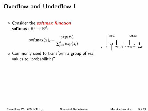
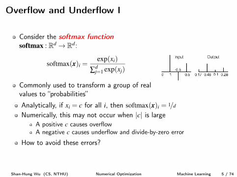
Consider the softmax function
softmax : Rd! Rd:
softmax(x)i =exp(xi)
Âdj=1
exp(xj)
Commonly used to transform a group of realvalues to “probabilities”
Analytically, if xi = c for all i, then softmax(x)i = 1/d
Numerically, this may not occur when |c| is largeA positive c causes overflowA negative c causes underflow and divide-by-zero error
How to avoid these errors?
Shan-Hung Wu (CS, NTHU) Numerical Optimization Machine Learning 5 / 74

Overflow and Underflow I
Consider the softmax function
softmax : Rd! Rd:
softmax(x)i =exp(xi)
Âdj=1
exp(xj)
Commonly used to transform a group of realvalues to “probabilities”Analytically, if xi = c for all i, then softmax(x)i = 1/d
Numerically, this may not occur when |c| is largeA positive c causes overflowA negative c causes underflow and divide-by-zero error
How to avoid these errors?
Shan-Hung Wu (CS, NTHU) Numerical Optimization Machine Learning 5 / 74
Overflow and Underflow II
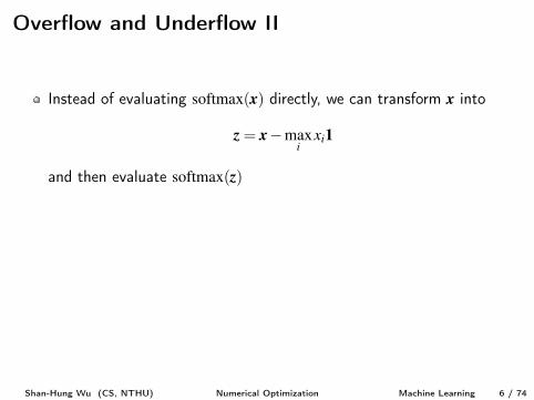
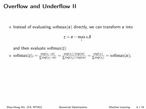
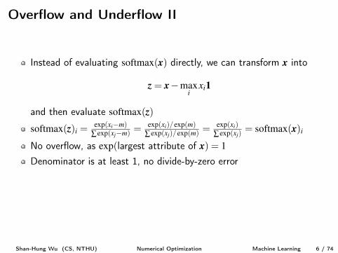
Instead of evaluating softmax(x) directly, we can transform x into
z = x�max
ixi1
and then evaluate softmax(z)
softmax(z)i =exp(xi�m)
Âexp(xj�m) =exp(xi)/exp(m)
Âexp(xj)/exp(m) =exp(xi)
Âexp(xj)= softmax(x)i
No overflow, as exp(largest attribute of x) = 1
Denominator is at least 1, no divide-by-zero errorWhat are the numerical issues of logsoftmax(z)? How to stabilize it?[Homework]
Shan-Hung Wu (CS, NTHU) Numerical Optimization Machine Learning 6 / 74
Overflow and Underflow II
Instead of evaluating softmax(x) directly, we can transform x into
z = x�max
ixi1
and then evaluate softmax(z)softmax(z)i =
exp(xi�m)Âexp(xj�m) =
exp(xi)/exp(m)Âexp(xj)/exp(m) =
exp(xi)Âexp(xj)
= softmax(x)i
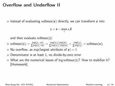
No overflow, as exp(largest attribute of x) = 1
Denominator is at least 1, no divide-by-zero error
What are the numerical issues of logsoftmax(z)? How to stabilize it?[Homework]
Shan-Hung Wu (CS, NTHU) Numerical Optimization Machine Learning 6 / 74
Overflow and Underflow II
Instead of evaluating softmax(x) directly, we can transform x into
z = x�max
ixi1
and then evaluate softmax(z)softmax(z)i =
exp(xi�m)Âexp(xj�m) =
exp(xi)/exp(m)Âexp(xj)/exp(m) =
exp(xi)Âexp(xj)
= softmax(x)i
No overflow, as exp(largest attribute of x) = 1
Denominator is at least 1, no divide-by-zero errorWhat are the numerical issues of logsoftmax(z)? How to stabilize it?[Homework]
Shan-Hung Wu (CS, NTHU) Numerical Optimization Machine Learning 6 / 74
Poor Conditioning I
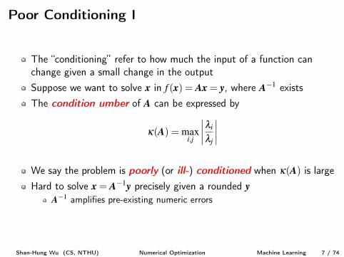
The “conditioning” refer to how much the input of a function canchange given a small change in the output
Suppose we want to solve x in f (x) = Ax = y, where A�1 existsThe condition umber of A can be expressed by
k(A) = max
i,j
����li
lj
����
We say the problem is poorly (or ill-) conditioned when k(A) is largeHard to solve x = A�1y precisely given a rounded y
A�1 amplifies pre-existing numeric errors
Shan-Hung Wu (CS, NTHU) Numerical Optimization Machine Learning 7 / 74
Poor Conditioning I
The “conditioning” refer to how much the input of a function canchange given a small change in the outputSuppose we want to solve x in f (x) = Ax = y, where A�1 exists
The condition umber of A can be expressed by
k(A) = max
i,j
����li
lj
����
We say the problem is poorly (or ill-) conditioned when k(A) is largeHard to solve x = A�1y precisely given a rounded y
A�1 amplifies pre-existing numeric errors
Shan-Hung Wu (CS, NTHU) Numerical Optimization Machine Learning 7 / 74
Poor Conditioning I
The “conditioning” refer to how much the input of a function canchange given a small change in the outputSuppose we want to solve x in f (x) = Ax = y, where A�1 existsThe condition umber of A can be expressed by
k(A) = max
i,j
����li
lj
����
We say the problem is poorly (or ill-) conditioned when k(A) is large
Hard to solve x = A�1y precisely given a rounded yA�1 amplifies pre-existing numeric errors
Shan-Hung Wu (CS, NTHU) Numerical Optimization Machine Learning 7 / 74
Poor Conditioning I
The “conditioning” refer to how much the input of a function canchange given a small change in the outputSuppose we want to solve x in f (x) = Ax = y, where A�1 existsThe condition umber of A can be expressed by
k(A) = max
i,j
����li
lj
����
We say the problem is poorly (or ill-) conditioned when k(A) is largeHard to solve x = A�1y precisely given a rounded y
A�1 amplifies pre-existing numeric errors
Shan-Hung Wu (CS, NTHU) Numerical Optimization Machine Learning 7 / 74
Poor Conditioning II
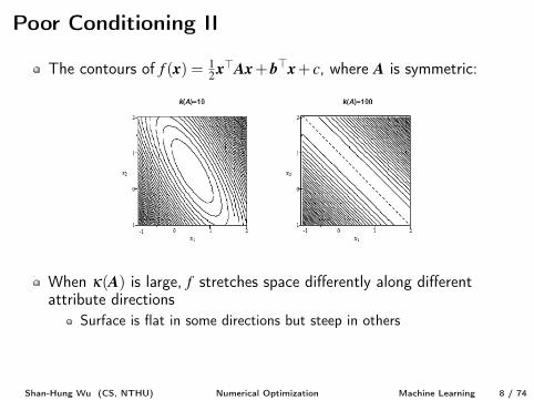
The contours of f (x) = 1
2
x>Ax+b>x+ c, where A is symmetric:
When k(A) is large, f stretches space differently along differentattribute directions
Surface is flat in some directions but steep in others
Hard to solve f 0(x) = 0) x = A�1b
Shan-Hung Wu (CS, NTHU) Numerical Optimization Machine Learning 8 / 74
Poor Conditioning II
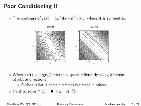
The contours of f (x) = 1
2
x>Ax+b>x+ c, where A is symmetric:
When k(A) is large, f stretches space differently along differentattribute directions
Surface is flat in some directions but steep in others
Hard to solve f 0(x) = 0) x = A�1b
Shan-Hung Wu (CS, NTHU) Numerical Optimization Machine Learning 8 / 74
Outline1 Numerical Computation2 Optimization Problems3 Unconstrained Optimization
Gradient DescentNewton’s Method
4 Optimization in ML: Stochastic Gradient DescentPerceptronAdalineStochastic Gradient Descent
5 Constrained Optimization6 Optimization in ML: Regularization
Linear RegressionPolynomial RegressionGeneralizability & Regularization
7 Duality*
Shan-Hung Wu (CS, NTHU) Numerical Optimization Machine Learning 9 / 74

Optimization Problems
An optimization problem is to minimize a cost function f : Rd!R:
minx f (x)subject to x 2 C
where C✓ Rd is called the feasible set containing feasible points
Or, maximizing an objective function
Maximizing f equals to minimizing �f
If C= Rd, we say the optimization problem is unconstrainedC can be a set of function constrains, i.e., C= {x : g(i)(x) 0}i
Sometimes, we single out equality constrainsC= {x : g(i)(x) 0,h(j)(x) = 0}i,j
Each equality constrain can be written as two inequality constrains
Shan-Hung Wu (CS, NTHU) Numerical Optimization Machine Learning 10 / 74
Optimization Problems
An optimization problem is to minimize a cost function f : Rd!R:
minx f (x)subject to x 2 C
where C✓ Rd is called the feasible set containing feasible points
Or, maximizing an objective function
Maximizing f equals to minimizing �f
If C= Rd, we say the optimization problem is unconstrained
C can be a set of function constrains, i.e., C= {x : g(i)(x) 0}i
Sometimes, we single out equality constrainsC= {x : g(i)(x) 0,h(j)(x) = 0}i,j
Each equality constrain can be written as two inequality constrains
Shan-Hung Wu (CS, NTHU) Numerical Optimization Machine Learning 10 / 74
Optimization Problems
An optimization problem is to minimize a cost function f : Rd!R:
minx f (x)subject to x 2 C
where C✓ Rd is called the feasible set containing feasible points
Or, maximizing an objective function
Maximizing f equals to minimizing �f
If C= Rd, we say the optimization problem is unconstrainedC can be a set of function constrains, i.e., C= {x : g(i)(x) 0}i
Sometimes, we single out equality constrainsC= {x : g(i)(x) 0,h(j)(x) = 0}i,j
Each equality constrain can be written as two inequality constrains
Shan-Hung Wu (CS, NTHU) Numerical Optimization Machine Learning 10 / 74
Optimization Problems
An optimization problem is to minimize a cost function f : Rd!R:
minx f (x)subject to x 2 C
where C✓ Rd is called the feasible set containing feasible points
Or, maximizing an objective function
Maximizing f equals to minimizing �f
If C= Rd, we say the optimization problem is unconstrainedC can be a set of function constrains, i.e., C= {x : g(i)(x) 0}i
Sometimes, we single out equality constrainsC= {x : g(i)(x) 0,h(j)(x) = 0}i,j
Each equality constrain can be written as two inequality constrains
Shan-Hung Wu (CS, NTHU) Numerical Optimization Machine Learning 10 / 74
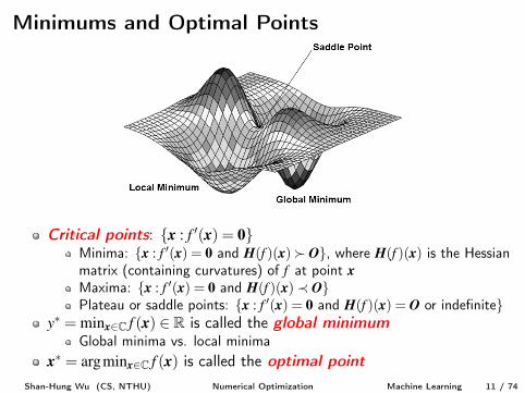
Minimums and Optimal Points
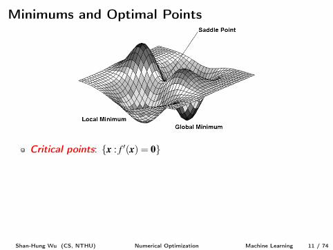
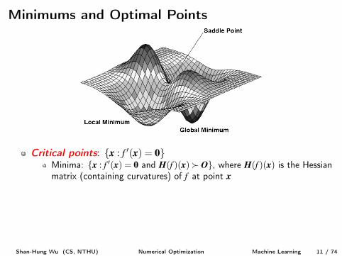
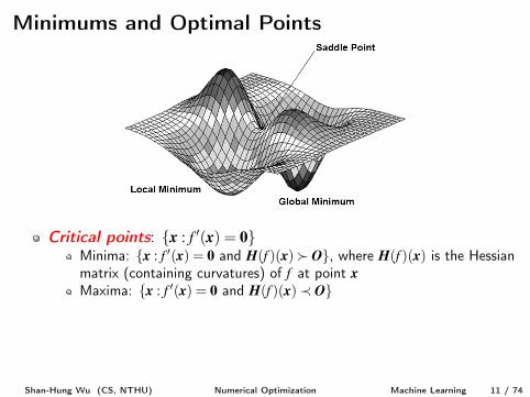
Critical points: {x : f 0(x) = 0}
Minima: {x : f 0(x) = 0 and H(f )(x)� O}, where H(f )(x) is the Hessianmatrix (containing curvatures) of f at point xMaxima: {x : f 0(x) = 0 and H(f )(x)� O}Plateau or saddle points: {x : f 0(x) = 0 and H(f )(x) = O or indefinite}
y⇤ = minx2C f (x) 2 R is called the global minimum
Global minima vs. local minimax⇤ = argminx2C f (x) is called the optimal point
Shan-Hung Wu (CS, NTHU) Numerical Optimization Machine Learning 11 / 74
Minimums and Optimal Points
Critical points: {x : f 0(x) = 0}Minima: {x : f 0(x) = 0 and H(f )(x)� O}, where H(f )(x) is the Hessianmatrix (containing curvatures) of f at point x
Maxima: {x : f 0(x) = 0 and H(f )(x)� O}Plateau or saddle points: {x : f 0(x) = 0 and H(f )(x) = O or indefinite}
y⇤ = minx2C f (x) 2 R is called the global minimum
Global minima vs. local minimax⇤ = argminx2C f (x) is called the optimal point
Shan-Hung Wu (CS, NTHU) Numerical Optimization Machine Learning 11 / 74
Minimums and Optimal Points
Critical points: {x : f 0(x) = 0}Minima: {x : f 0(x) = 0 and H(f )(x)� O}, where H(f )(x) is the Hessianmatrix (containing curvatures) of f at point xMaxima: {x : f 0(x) = 0 and H(f )(x)� O}
Plateau or saddle points: {x : f 0(x) = 0 and H(f )(x) = O or indefinite}y⇤ = minx2C f (x) 2 R is called the global minimum
Global minima vs. local minimax⇤ = argminx2C f (x) is called the optimal point
Shan-Hung Wu (CS, NTHU) Numerical Optimization Machine Learning 11 / 74

Minimums and Optimal Points
Critical points: {x : f 0(x) = 0}Minima: {x : f 0(x) = 0 and H(f )(x)� O}, where H(f )(x) is the Hessianmatrix (containing curvatures) of f at point xMaxima: {x : f 0(x) = 0 and H(f )(x)� O}Plateau or saddle points: {x : f 0(x) = 0 and H(f )(x) = O or indefinite}
y⇤ = minx2C f (x) 2 R is called the global minimum
Global minima vs. local minimax⇤ = argminx2C f (x) is called the optimal point
Shan-Hung Wu (CS, NTHU) Numerical Optimization Machine Learning 11 / 74
Minimums and Optimal Points
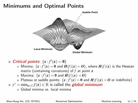
Critical points: {x : f 0(x) = 0}Minima: {x : f 0(x) = 0 and H(f )(x)� O}, where H(f )(x) is the Hessianmatrix (containing curvatures) of f at point xMaxima: {x : f 0(x) = 0 and H(f )(x)� O}Plateau or saddle points: {x : f 0(x) = 0 and H(f )(x) = O or indefinite}
y⇤ = minx2C f (x) 2 R is called the global minimum
Global minima vs. local minima
x⇤ = argminx2C f (x) is called the optimal point
Shan-Hung Wu (CS, NTHU) Numerical Optimization Machine Learning 11 / 74
Minimums and Optimal Points
Critical points: {x : f 0(x) = 0}Minima: {x : f 0(x) = 0 and H(f )(x)� O}, where H(f )(x) is the Hessianmatrix (containing curvatures) of f at point xMaxima: {x : f 0(x) = 0 and H(f )(x)� O}Plateau or saddle points: {x : f 0(x) = 0 and H(f )(x) = O or indefinite}
y⇤ = minx2C f (x) 2 R is called the global minimum
Global minima vs. local minimax⇤ = argminx2C f (x) is called the optimal point
Shan-Hung Wu (CS, NTHU) Numerical Optimization Machine Learning 11 / 74
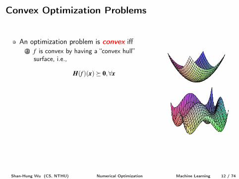
Convex Optimization Problems
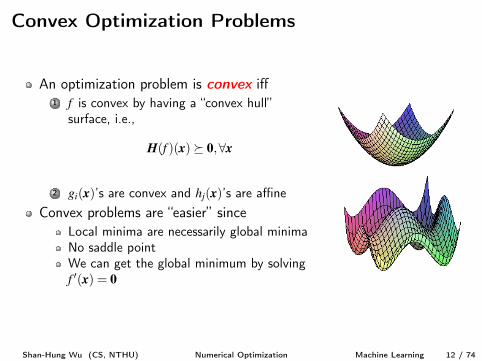
An optimization problem is convex iff1 f is convex by having a “convex hull”
surface, i.e.,
H(f )(x)⌫ 0,8x
2 gi(x)’s are convex and hj(x)’s are affineConvex problems are “easier” since
Local minima are necessarily global minimaNo saddle pointWe can get the global minimum by solvingf 0(x) = 0
Shan-Hung Wu (CS, NTHU) Numerical Optimization Machine Learning 12 / 74
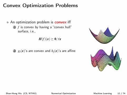
Convex Optimization Problems
An optimization problem is convex iff1 f is convex by having a “convex hull”
surface, i.e.,
H(f )(x)⌫ 0,8x
2 gi(x)’s are convex and hj(x)’s are affine
Convex problems are “easier” sinceLocal minima are necessarily global minimaNo saddle pointWe can get the global minimum by solvingf 0(x) = 0
Shan-Hung Wu (CS, NTHU) Numerical Optimization Machine Learning 12 / 74
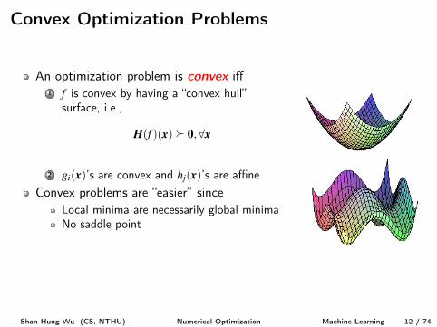
Convex Optimization Problems
An optimization problem is convex iff1 f is convex by having a “convex hull”
surface, i.e.,
H(f )(x)⌫ 0,8x
2 gi(x)’s are convex and hj(x)’s are affineConvex problems are “easier” since
Local minima are necessarily global minimaNo saddle point
We can get the global minimum by solvingf 0(x) = 0
Shan-Hung Wu (CS, NTHU) Numerical Optimization Machine Learning 12 / 74
Convex Optimization Problems
An optimization problem is convex iff1 f is convex by having a “convex hull”
surface, i.e.,
H(f )(x)⌫ 0,8x
2 gi(x)’s are convex and hj(x)’s are affineConvex problems are “easier” since
Local minima are necessarily global minimaNo saddle pointWe can get the global minimum by solvingf 0(x) = 0
Shan-Hung Wu (CS, NTHU) Numerical Optimization Machine Learning 12 / 74
Analytical Solutions vs. Numerical Solutions I
Consider the problem:
argmin
x
1
2
�kAx�bk2 +lkxk2
�
Analytical solutions?
The cost function f (x) = 1
2
x>�A>A+l I
�x�b>Ax+ 1
2
kbk2 is convex
Solving f 0(x) = x>�A>A+l I
��b>A = 0, we have
x⇤ =⇣
A>A+l I⌘�1
A>b
Shan-Hung Wu (CS, NTHU) Numerical Optimization Machine Learning 13 / 74
Analytical Solutions vs. Numerical Solutions I
Consider the problem:
argmin
x
1
2
�kAx�bk2 +lkxk2
�
Analytical solutions?The cost function f (x) = 1
2
x>�A>A+l I
�x�b>Ax+ 1
2
kbk2 is convex
Solving f 0(x) = x>�A>A+l I
��b>A = 0, we have
x⇤ =⇣
A>A+l I⌘�1
A>b
Shan-Hung Wu (CS, NTHU) Numerical Optimization Machine Learning 13 / 74
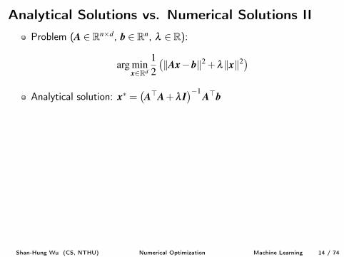
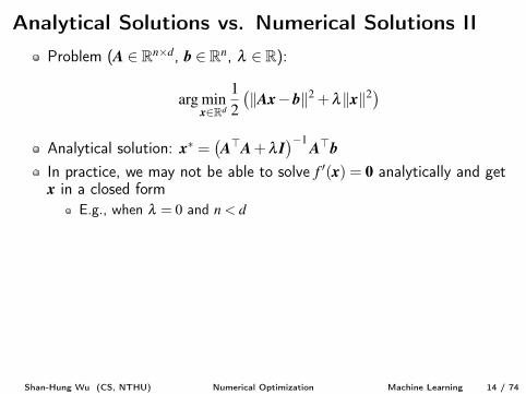
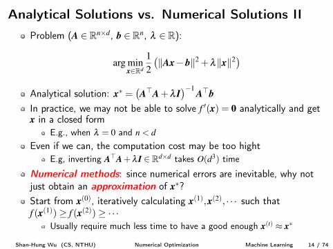
Analytical Solutions vs. Numerical Solutions IIProblem (A 2 Rn⇥d, b 2 Rn, l 2 R):
arg min
x2Rd
1
2
�kAx�bk2 +lkxk2
�
Analytical solution: x⇤ =�A>A+l I
��1 A>b
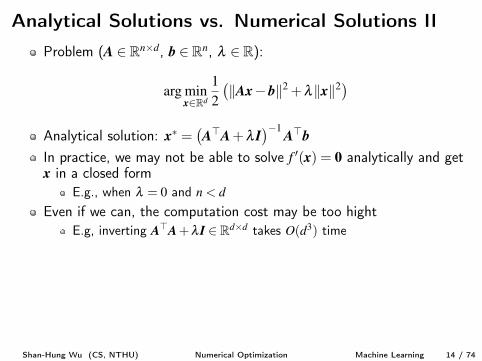
In practice, we may not be able to solve f 0(x) = 0 analytically and getx in a closed form
E.g., when l = 0 and n < d
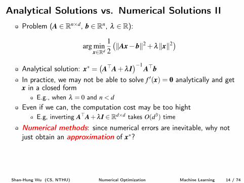
Even if we can, the computation cost may be too hightE.g, inverting A>A+l I 2 Rd⇥d takes O(d3) time
Numerical methods: since numerical errors are inevitable, why notjust obtain an approximation of x⇤?Start from x(0), iteratively calculating x(1),x(2), · · · such thatf (x(1))� f (x(2))� · · ·
Usually require much less time to have a good enough x(t) ⇡ x⇤
Shan-Hung Wu (CS, NTHU) Numerical Optimization Machine Learning 14 / 74
Analytical Solutions vs. Numerical Solutions IIProblem (A 2 Rn⇥d, b 2 Rn, l 2 R):
arg min
x2Rd
1
2
�kAx�bk2 +lkxk2
�
Analytical solution: x⇤ =�A>A+l I
��1 A>bIn practice, we may not be able to solve f 0(x) = 0 analytically and getx in a closed form
E.g., when l = 0 and n < d
Even if we can, the computation cost may be too hightE.g, inverting A>A+l I 2 Rd⇥d takes O(d3) time
Numerical methods: since numerical errors are inevitable, why notjust obtain an approximation of x⇤?
Start from x(0), iteratively calculating x(1),x(2), · · · such thatf (x(1))� f (x(2))� · · ·
Usually require much less time to have a good enough x(t) ⇡ x⇤
Shan-Hung Wu (CS, NTHU) Numerical Optimization Machine Learning 14 / 74
Analytical Solutions vs. Numerical Solutions IIProblem (A 2 Rn⇥d, b 2 Rn, l 2 R):
arg min
x2Rd
1
2
�kAx�bk2 +lkxk2
�
Analytical solution: x⇤ =�A>A+l I
��1 A>bIn practice, we may not be able to solve f 0(x) = 0 analytically and getx in a closed form
E.g., when l = 0 and n < d
Even if we can, the computation cost may be too hightE.g, inverting A>A+l I 2 Rd⇥d takes O(d3) time
Numerical methods: since numerical errors are inevitable, why notjust obtain an approximation of x⇤?Start from x(0), iteratively calculating x(1),x(2), · · · such thatf (x(1))� f (x(2))� · · ·
Usually require much less time to have a good enough x(t) ⇡ x⇤
Shan-Hung Wu (CS, NTHU) Numerical Optimization Machine Learning 14 / 74
Outline1 Numerical Computation2 Optimization Problems3 Unconstrained Optimization
Gradient DescentNewton’s Method
4 Optimization in ML: Stochastic Gradient DescentPerceptronAdalineStochastic Gradient Descent
5 Constrained Optimization6 Optimization in ML: Regularization
Linear RegressionPolynomial RegressionGeneralizability & Regularization
7 Duality*
Shan-Hung Wu (CS, NTHU) Numerical Optimization Machine Learning 15 / 74
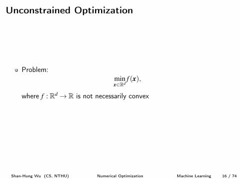
Unconstrained Optimization
Problem:min
x2Rdf (x),
where f : Rd! R is not necessarily convex
Shan-Hung Wu (CS, NTHU) Numerical Optimization Machine Learning 16 / 74
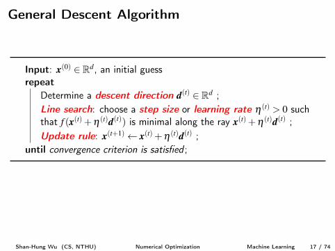
General Descent Algorithm
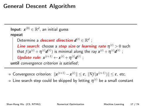
Input: x(0) 2 Rd, an initial guessrepeat
Determine a descent direction d(t) 2 Rd ;Line search: choose a step size or learning rate h(t) > 0 suchthat f (x(t) +h(t)d(t)) is minimal along the ray x(t) +h(t)d(t) ;Update rule: x(t+1) x(t) +h(t)d(t) ;
until convergence criterion is satisfied ;
Convergence criterion: kx(t+1)�x(t)k e , k—f (x(t+1))k e , etc.Line search step could be skipped by letting h(t) be a small constant
Shan-Hung Wu (CS, NTHU) Numerical Optimization Machine Learning 17 / 74
General Descent Algorithm
Input: x(0) 2 Rd, an initial guessrepeat
Determine a descent direction d(t) 2 Rd ;Line search: choose a step size or learning rate h(t) > 0 suchthat f (x(t) +h(t)d(t)) is minimal along the ray x(t) +h(t)d(t) ;Update rule: x(t+1) x(t) +h(t)d(t) ;
until convergence criterion is satisfied ;
Convergence criterion: kx(t+1)�x(t)k e , k—f (x(t+1))k e , etc.Line search step could be skipped by letting h(t) be a small constant
Shan-Hung Wu (CS, NTHU) Numerical Optimization Machine Learning 17 / 74
Outline1 Numerical Computation2 Optimization Problems3 Unconstrained Optimization
Gradient DescentNewton’s Method
4 Optimization in ML: Stochastic Gradient DescentPerceptronAdalineStochastic Gradient Descent
5 Constrained Optimization6 Optimization in ML: Regularization
Linear RegressionPolynomial RegressionGeneralizability & Regularization
7 Duality*
Shan-Hung Wu (CS, NTHU) Numerical Optimization Machine Learning 18 / 74
Gradient Descent I
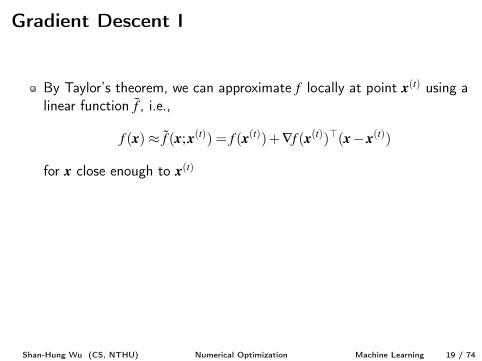
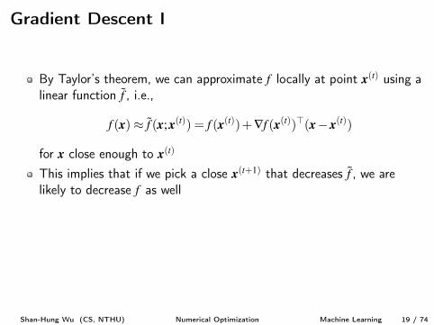
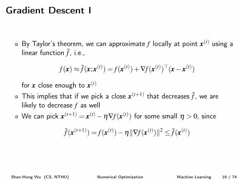
By Taylor’s theorem, we can approximate f locally at point x(t) using alinear function ˜f , i.e.,
f (x)⇡ ˜f (x;x(t)) = f (x(t))+—f (x(t))>(x�x(t))
for x close enough to x(t)
This implies that if we pick a close x(t+1) that decreases ˜f , we arelikely to decrease f as wellWe can pick x(t+1) = x(t)�h—f (x(t)) for some small h > 0, since
˜f (x(t+1)) = f (x(t))�hk—f (x(t))k2 ˜f (x(t))
Shan-Hung Wu (CS, NTHU) Numerical Optimization Machine Learning 19 / 74
Gradient Descent I
By Taylor’s theorem, we can approximate f locally at point x(t) using alinear function ˜f , i.e.,
f (x)⇡ ˜f (x;x(t)) = f (x(t))+—f (x(t))>(x�x(t))
for x close enough to x(t)
This implies that if we pick a close x(t+1) that decreases ˜f , we arelikely to decrease f as well
We can pick x(t+1) = x(t)�h—f (x(t)) for some small h > 0, since
˜f (x(t+1)) = f (x(t))�hk—f (x(t))k2 ˜f (x(t))
Shan-Hung Wu (CS, NTHU) Numerical Optimization Machine Learning 19 / 74
Gradient Descent I
By Taylor’s theorem, we can approximate f locally at point x(t) using alinear function ˜f , i.e.,
f (x)⇡ ˜f (x;x(t)) = f (x(t))+—f (x(t))>(x�x(t))
for x close enough to x(t)
This implies that if we pick a close x(t+1) that decreases ˜f , we arelikely to decrease f as wellWe can pick x(t+1) = x(t)�h—f (x(t)) for some small h > 0, since
˜f (x(t+1)) = f (x(t))�hk—f (x(t))k2 ˜f (x(t))
Shan-Hung Wu (CS, NTHU) Numerical Optimization Machine Learning 19 / 74
Gradient Descent II
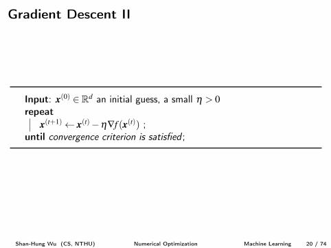
Input: x(0) 2 Rd an initial guess, a small h > 0
repeatx(t+1) x(t)�h—f (x(t)) ;
until convergence criterion is satisfied ;
Shan-Hung Wu (CS, NTHU) Numerical Optimization Machine Learning 20 / 74
Is Negative Gradient a Good Direction? I
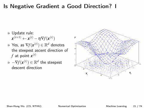
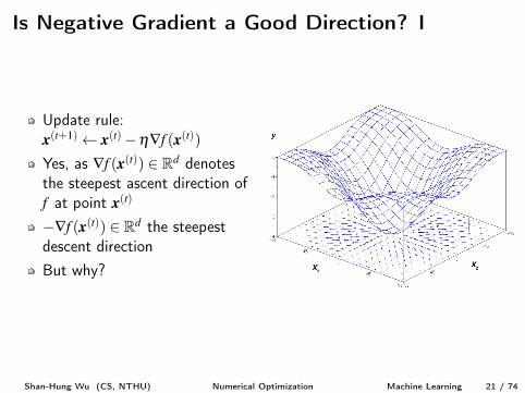
Update rule:x(t+1) x(t)�h—f (x(t))
Yes, as —f (x(t)) 2 Rd denotesthe steepest ascent direction off at point x(t)
�—f (x(t)) 2 Rd the steepestdescent directionBut why?
Shan-Hung Wu (CS, NTHU) Numerical Optimization Machine Learning 21 / 74
Is Negative Gradient a Good Direction? I
Update rule:x(t+1) x(t)�h—f (x(t))Yes, as —f (x(t)) 2 Rd denotesthe steepest ascent direction off at point x(t)
�—f (x(t)) 2 Rd the steepestdescent direction
But why?
Shan-Hung Wu (CS, NTHU) Numerical Optimization Machine Learning 21 / 74
Is Negative Gradient a Good Direction? I
Update rule:x(t+1) x(t)�h—f (x(t))Yes, as —f (x(t)) 2 Rd denotesthe steepest ascent direction off at point x(t)
�—f (x(t)) 2 Rd the steepestdescent directionBut why?
Shan-Hung Wu (CS, NTHU) Numerical Optimization Machine Learning 21 / 74
Is Negative Gradient a Good Direction? II
Consider the slope of f in a given direction u at point x(t)
This is the directional derivative of f , i.e., the derivative of functionf (x(t) + eu) with respect to e , evaluated at e = 0
By the chain rule, we have ∂∂e f (x(t) + eu) = —f (x(t) + eu)>u, which
equals to —f (x(t))>u when e = 0
Theorem (Chain Rule)
Let g : R! Rdand f : Rd! R, then
(f �g)0(x) = f 0(g(x))g0(x) = —f (g(x))>
2
64g0
1
(x).
.
.
g0n(x)
3
75 .
Shan-Hung Wu (CS, NTHU) Numerical Optimization Machine Learning 22 / 74
Is Negative Gradient a Good Direction? III
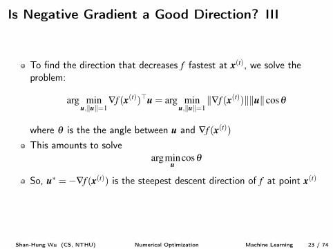
To find the direction that decreases f fastest at x(t), we solve theproblem:
arg min
u,kuk=1
—f (x(t))>u = arg min
u,kuk=1
k—f (x(t))kkukcosq
where q is the the angle between u and —f (x(t))
This amounts to solveargmin
ucosq
So, u⇤ =�—f (x(t)) is the steepest descent direction of f at point x(t)
Shan-Hung Wu (CS, NTHU) Numerical Optimization Machine Learning 23 / 74
Is Negative Gradient a Good Direction? III
To find the direction that decreases f fastest at x(t), we solve theproblem:
arg min
u,kuk=1
—f (x(t))>u = arg min
u,kuk=1
k—f (x(t))kkukcosq
where q is the the angle between u and —f (x(t))This amounts to solve
argmin
ucosq
So, u⇤ =�—f (x(t)) is the steepest descent direction of f at point x(t)
Shan-Hung Wu (CS, NTHU) Numerical Optimization Machine Learning 23 / 74
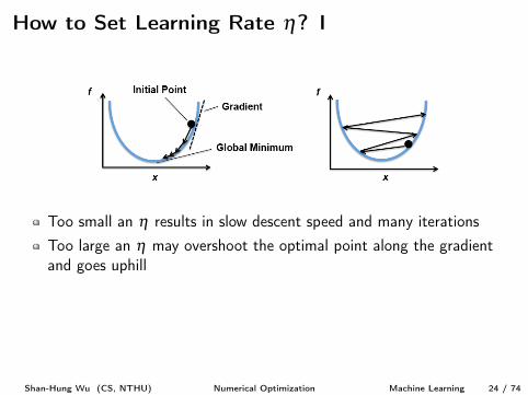
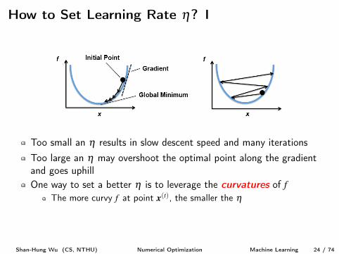
How to Set Learning Rate h? I
Too small an h results in slow descent speed and many iterationsToo large an h may overshoot the optimal point along the gradientand goes uphill
One way to set a better h is to leverage the curvatures of fThe more curvy f at point x(t), the smaller the h
Shan-Hung Wu (CS, NTHU) Numerical Optimization Machine Learning 24 / 74
How to Set Learning Rate h? I
Too small an h results in slow descent speed and many iterationsToo large an h may overshoot the optimal point along the gradientand goes uphillOne way to set a better h is to leverage the curvatures of f
The more curvy f at point x(t), the smaller the h
Shan-Hung Wu (CS, NTHU) Numerical Optimization Machine Learning 24 / 74
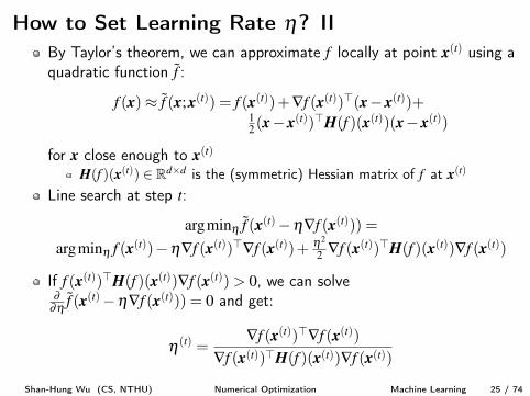
How to Set Learning Rate h? IIBy Taylor’s theorem, we can approximate f locally at point x(t) using aquadratic function ˜f :
f (x)⇡ ˜f (x;x(t)) = f (x(t))+—f (x(t))>(x�x(t))+1
2
(x�x(t))>H(f )(x(t))(x�x(t))
for x close enough to x(t)H(f )(x(t)) 2 Rd⇥d is the (symmetric) Hessian matrix of f at x(t)
Line search at step t:
argminh ˜f (x(t)�h—f (x(t))) =argminh f (x(t))�h—f (x(t))>—f (x(t))+ h2
2
—f (x(t))>H(f )(x(t))—f (x(t))
If f (x(t))>H(f )(x(t))—f (x(t))> 0, we can solve∂
∂h˜f (x(t)�h—f (x(t))) = 0 and get:
h(t) =—f (x(t))>—f (x(t))
—f (x(t))>H(f )(x(t))—f (x(t))
Shan-Hung Wu (CS, NTHU) Numerical Optimization Machine Learning 25 / 74
Problems of Gradient Descent
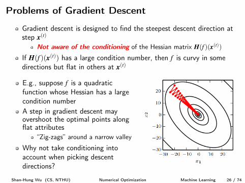
Gradient descent is designed to find the steepest descent direction atstep x(t)
Not aware of the conditioning of the Hessian matrix H(f )(x(t))
If H(f )(x(t)) has a large condition number, then f is curvy in somedirections but flat in others at x(t)
E.g., suppose f is a quadraticfunction whose Hessian has a largecondition numberA step in gradient descent mayovershoot the optimal points alongflat attributes
“Zig-zags” around a narrow valley
Why not take conditioning intoaccount when picking descentdirections?
Shan-Hung Wu (CS, NTHU) Numerical Optimization Machine Learning 26 / 74
Problems of Gradient Descent
Gradient descent is designed to find the steepest descent direction atstep x(t)
Not aware of the conditioning of the Hessian matrix H(f )(x(t))If H(f )(x(t)) has a large condition number, then f is curvy in somedirections but flat in others at x(t)
E.g., suppose f is a quadraticfunction whose Hessian has a largecondition numberA step in gradient descent mayovershoot the optimal points alongflat attributes
“Zig-zags” around a narrow valley
Why not take conditioning intoaccount when picking descentdirections?
Shan-Hung Wu (CS, NTHU) Numerical Optimization Machine Learning 26 / 74
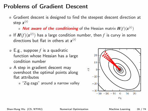
Outline1 Numerical Computation2 Optimization Problems3 Unconstrained Optimization
Gradient DescentNewton’s Method
4 Optimization in ML: Stochastic Gradient DescentPerceptronAdalineStochastic Gradient Descent
5 Constrained Optimization6 Optimization in ML: Regularization
Linear RegressionPolynomial RegressionGeneralizability & Regularization
7 Duality*
Shan-Hung Wu (CS, NTHU) Numerical Optimization Machine Learning 27 / 74
Newton’s Method I
By Taylor’s theorem, we can approximate f locally at point x(t) using aquadratic function ˜f , i.e.,
f (x)⇡ ˜f (x;x(t)) = f (x(t))+—f (x(t))>(x�x(t))+1
2
(x�x(t))>H(f )(x(t))(x�x(t))
for x close enough to x(t)
If f is strictly convex (i.e., H(f )(a)� O,8a), we can find x(t+1) thatminimizes ˜f in order to decrease f
Solving —˜f (x(t+1);x(t)) = 0, we have
x(t+1) = x(t)�H(f )(x(t))�1—f (x(t))
H(f )(x(t))�1 as a “corrector” to the negative gradient
Shan-Hung Wu (CS, NTHU) Numerical Optimization Machine Learning 28 / 74
Newton’s Method II
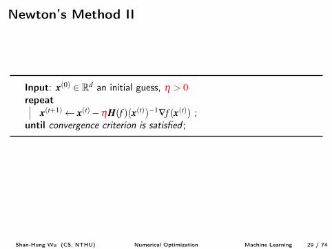
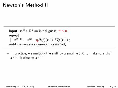
Input: x(0) 2 Rd an initial guess, h > 0
repeatx(t+1) x(t)�hH(f )(x(t))�1—f (x(t)) ;
until convergence criterion is satisfied ;
In practice, we multiply the shift by a small h > 0 to make sure thatx(t+1) is close to x(t)
Shan-Hung Wu (CS, NTHU) Numerical Optimization Machine Learning 29 / 74
Newton’s Method II
Input: x(0) 2 Rd an initial guess, h > 0
repeatx(t+1) x(t)�hH(f )(x(t))�1—f (x(t)) ;
until convergence criterion is satisfied ;
In practice, we multiply the shift by a small h > 0 to make sure thatx(t+1) is close to x(t)
Shan-Hung Wu (CS, NTHU) Numerical Optimization Machine Learning 29 / 74
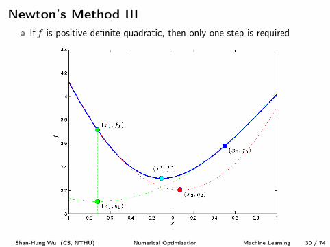
Newton’s Method IIIIf f is positive definite quadratic, then only one step is required
Shan-Hung Wu (CS, NTHU) Numerical Optimization Machine Learning 30 / 74
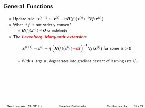
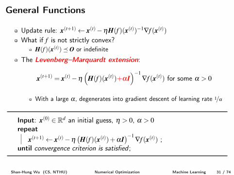
General Functions
Update rule: x(t+1) x(t)�hH(f )(x(t))�1—f (x(t))What if f is not strictly convex?
H(f )(x(t))� O or indefinite
The Levenberg–Marquardt extension:
x(t+1) = x(t)�h⇣
H(f )(x(t))+aI⌘�1
—f (x(t)) for some a > 0
With a large a, degenerates into gradient descent of learning rate 1/a
Input: x(0) 2 Rd an initial guess, h > 0, a > 0
repeatx(t+1) x(t)�h
�H(f )(x(t))+aI
��1 —f (x(t)) ;until convergence criterion is satisfied ;
Shan-Hung Wu (CS, NTHU) Numerical Optimization Machine Learning 31 / 74
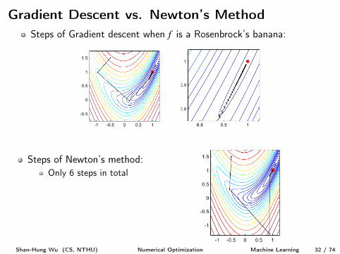
Gradient Descent vs. Newton’s MethodSteps of Gradient descent when f is a Rosenbrock’s banana:
Steps of Newton’s method:Only 6 steps in total
Shan-Hung Wu (CS, NTHU) Numerical Optimization Machine Learning 32 / 74
Problems of Newton’s Method
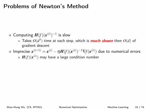
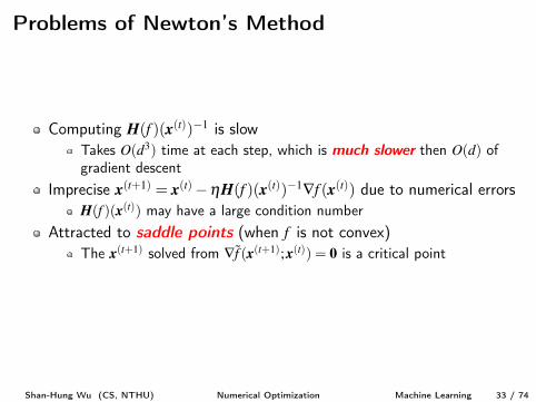
Computing H(f )(x(t))�1 is slowTakes O(d3) time at each step, which is much slower then O(d) ofgradient descent
Imprecise x(t+1) = x(t)�hH(f )(x(t))�1—f (x(t)) due to numerical errorsH(f )(x(t)) may have a large condition number
Attracted to saddle points (when f is not convex)The x(t+1) solved from —˜f (x(t+1)
;x(t)) = 0 is a critical point
Shan-Hung Wu (CS, NTHU) Numerical Optimization Machine Learning 33 / 74
Problems of Newton’s Method
Computing H(f )(x(t))�1 is slowTakes O(d3) time at each step, which is much slower then O(d) ofgradient descent
Imprecise x(t+1) = x(t)�hH(f )(x(t))�1—f (x(t)) due to numerical errorsH(f )(x(t)) may have a large condition number
Attracted to saddle points (when f is not convex)The x(t+1) solved from —˜f (x(t+1)
;x(t)) = 0 is a critical point
Shan-Hung Wu (CS, NTHU) Numerical Optimization Machine Learning 33 / 74
Outline1 Numerical Computation2 Optimization Problems3 Unconstrained Optimization
Gradient DescentNewton’s Method
4 Optimization in ML: Stochastic Gradient DescentPerceptronAdalineStochastic Gradient Descent
5 Constrained Optimization6 Optimization in ML: Regularization
Linear RegressionPolynomial RegressionGeneralizability & Regularization
7 Duality*
Shan-Hung Wu (CS, NTHU) Numerical Optimization Machine Learning 34 / 74
Who is Afraid of Non-convexity?
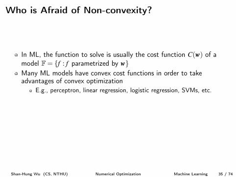
In ML, the function to solve is usually the cost function C(w) of amodel F= {f : f parametrized by w}
Many ML models have convex cost functions in order to takeadvantages of convex optimization
E.g., perceptron, linear regression, logistic regression, SVMs, etc.However, in deep learning, the cost function of a neural network istypically not convex
We will discuss techniques that tackle non-convexity later
Shan-Hung Wu (CS, NTHU) Numerical Optimization Machine Learning 35 / 74
Who is Afraid of Non-convexity?
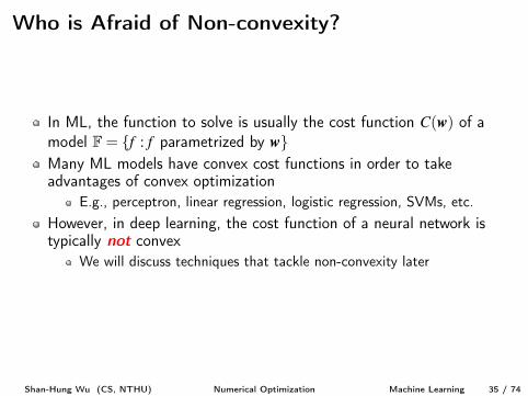
In ML, the function to solve is usually the cost function C(w) of amodel F= {f : f parametrized by w}Many ML models have convex cost functions in order to takeadvantages of convex optimization
E.g., perceptron, linear regression, logistic regression, SVMs, etc.
However, in deep learning, the cost function of a neural network istypically not convex
We will discuss techniques that tackle non-convexity later
Shan-Hung Wu (CS, NTHU) Numerical Optimization Machine Learning 35 / 74
Who is Afraid of Non-convexity?
In ML, the function to solve is usually the cost function C(w) of amodel F= {f : f parametrized by w}Many ML models have convex cost functions in order to takeadvantages of convex optimization
E.g., perceptron, linear regression, logistic regression, SVMs, etc.However, in deep learning, the cost function of a neural network istypically not convex
We will discuss techniques that tackle non-convexity later
Shan-Hung Wu (CS, NTHU) Numerical Optimization Machine Learning 35 / 74
Assumption on Cost Functions
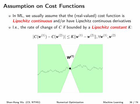
In ML, we usually assume that the (real-valued) cost function isLipschitz continuous and/or have Lipschitz continuous derivativesI.e., the rate of change of C if bounded by a Lipschitz constant K:
|C(w(1))�C(w(2))| Kkw(1)�w(2)k,8w(1),w(2)
Shan-Hung Wu (CS, NTHU) Numerical Optimization Machine Learning 36 / 74
Outline1 Numerical Computation2 Optimization Problems3 Unconstrained Optimization
Gradient DescentNewton’s Method
4 Optimization in ML: Stochastic Gradient DescentPerceptronAdalineStochastic Gradient Descent
5 Constrained Optimization6 Optimization in ML: Regularization
Linear RegressionPolynomial RegressionGeneralizability & Regularization
7 Duality*
Shan-Hung Wu (CS, NTHU) Numerical Optimization Machine Learning 37 / 74
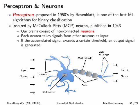
Perceptron & NeuronsPerceptron, proposed in 1950’s by Rosenblatt, is one of the first MLalgorithms for binary classification
Inspired by McCullock-Pitts (MCP) neuron, published in 1943Our brains consist of interconnected neurons
Each neuron takes signals from other neurons as inputIf the accumulated signal exceeds a certain threshold, an output signalis generated
Shan-Hung Wu (CS, NTHU) Numerical Optimization Machine Learning 38 / 74
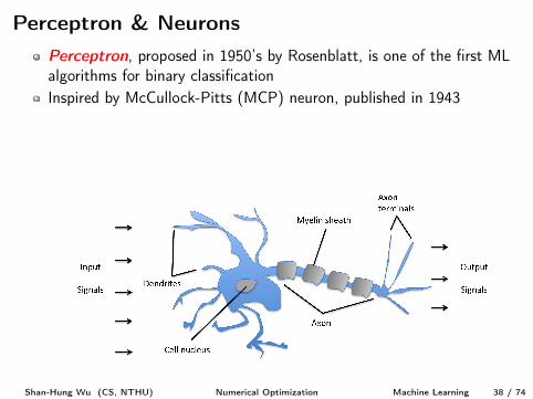
Perceptron & NeuronsPerceptron, proposed in 1950’s by Rosenblatt, is one of the first MLalgorithms for binary classificationInspired by McCullock-Pitts (MCP) neuron, published in 1943
Our brains consist of interconnected neurons
Each neuron takes signals from other neurons as inputIf the accumulated signal exceeds a certain threshold, an output signalis generated
Shan-Hung Wu (CS, NTHU) Numerical Optimization Machine Learning 38 / 74
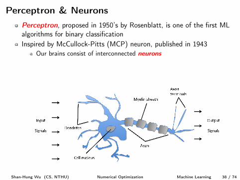
Perceptron & NeuronsPerceptron, proposed in 1950’s by Rosenblatt, is one of the first MLalgorithms for binary classificationInspired by McCullock-Pitts (MCP) neuron, published in 1943
Our brains consist of interconnected neurons
Each neuron takes signals from other neurons as inputIf the accumulated signal exceeds a certain threshold, an output signalis generated
Shan-Hung Wu (CS, NTHU) Numerical Optimization Machine Learning 38 / 74
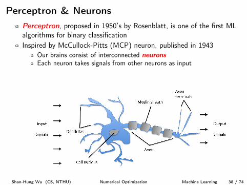
Perceptron & NeuronsPerceptron, proposed in 1950’s by Rosenblatt, is one of the first MLalgorithms for binary classificationInspired by McCullock-Pitts (MCP) neuron, published in 1943
Our brains consist of interconnected neurons
Each neuron takes signals from other neurons as input
If the accumulated signal exceeds a certain threshold, an output signalis generated
Shan-Hung Wu (CS, NTHU) Numerical Optimization Machine Learning 38 / 74
Perceptron & NeuronsPerceptron, proposed in 1950’s by Rosenblatt, is one of the first MLalgorithms for binary classificationInspired by McCullock-Pitts (MCP) neuron, published in 1943
Our brains consist of interconnected neurons
Each neuron takes signals from other neurons as inputIf the accumulated signal exceeds a certain threshold, an output signalis generated
Shan-Hung Wu (CS, NTHU) Numerical Optimization Machine Learning 38 / 74
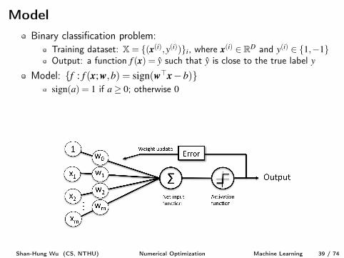
ModelBinary classification problem:
Training dataset: X= {(x(i),y(i))}i, where x(i) 2 RD and y(i) 2 {1,�1}Output: a function f (x) = y such that y is close to the true label y
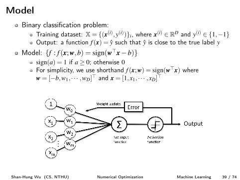
Model: {f : f (x;w,b) = sign(w>x�b)}sign(a) = 1 if a� 0; otherwise 0
For simplicity, we use shorthand f (x;w) = sign(w>x) wherew = [�b,w
1
, · · · ,wD]> and x = [1,x1
, · · · ,xD]>
Shan-Hung Wu (CS, NTHU) Numerical Optimization Machine Learning 39 / 74
ModelBinary classification problem:
Training dataset: X= {(x(i),y(i))}i, where x(i) 2 RD and y(i) 2 {1,�1}Output: a function f (x) = y such that y is close to the true label y
Model: {f : f (x;w,b) = sign(w>x�b)}sign(a) = 1 if a� 0; otherwise 0
For simplicity, we use shorthand f (x;w) = sign(w>x) wherew = [�b,w
1
, · · · ,wD]> and x = [1,x1
, · · · ,xD]>
Shan-Hung Wu (CS, NTHU) Numerical Optimization Machine Learning 39 / 74
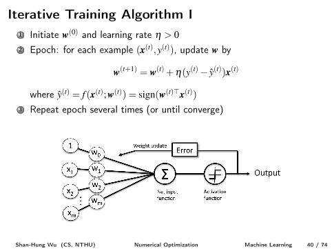
Iterative Training Algorithm I1 Initiate w(0) and learning rate h > 0
2 Epoch: for each example (x(t),y(t)), update w by
w(t+1) = w(t) +h(y(t)� y(t))x(t)
where y(t) = f (x(t);w(t)) = sign(w(t)>x(t))3 Repeat epoch several times (or until converge)
Shan-Hung Wu (CS, NTHU) Numerical Optimization Machine Learning 40 / 74
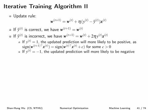
Iterative Training Algorithm IIUpdate rule:
w(t+1) = w(t) +h(y(t)� y(t))x(t)
If y(t) is correct, we have w(t+1) = w(t)
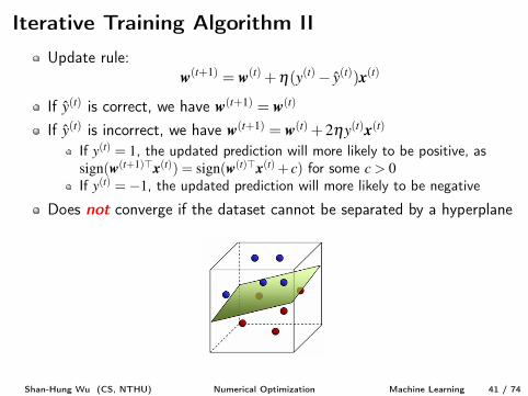
If y(t) is incorrect, we have w(t+1) = w(t) +2hy(t)x(t)If y(t) = 1, the updated prediction will more likely to be positive, assign(w(t+1)>x(t)) = sign(w(t)>x(t) + c) for some c > 0
If y(t) =�1, the updated prediction will more likely to be negative
Does not converge if the dataset cannot be separated by a hyperplane
Shan-Hung Wu (CS, NTHU) Numerical Optimization Machine Learning 41 / 74
Iterative Training Algorithm IIUpdate rule:
w(t+1) = w(t) +h(y(t)� y(t))x(t)
If y(t) is correct, we have w(t+1) = w(t)
If y(t) is incorrect, we have w(t+1) = w(t) +2hy(t)x(t)
If y(t) = 1, the updated prediction will more likely to be positive, assign(w(t+1)>x(t)) = sign(w(t)>x(t) + c) for some c > 0
If y(t) =�1, the updated prediction will more likely to be negative
Does not converge if the dataset cannot be separated by a hyperplane
Shan-Hung Wu (CS, NTHU) Numerical Optimization Machine Learning 41 / 74
Iterative Training Algorithm IIUpdate rule:
w(t+1) = w(t) +h(y(t)� y(t))x(t)
If y(t) is correct, we have w(t+1) = w(t)
If y(t) is incorrect, we have w(t+1) = w(t) +2hy(t)x(t)If y(t) = 1, the updated prediction will more likely to be positive, assign(w(t+1)>x(t)) = sign(w(t)>x(t) + c) for some c > 0
If y(t) =�1, the updated prediction will more likely to be negative
Does not converge if the dataset cannot be separated by a hyperplane
Shan-Hung Wu (CS, NTHU) Numerical Optimization Machine Learning 41 / 74
Iterative Training Algorithm IIUpdate rule:
w(t+1) = w(t) +h(y(t)� y(t))x(t)
If y(t) is correct, we have w(t+1) = w(t)
If y(t) is incorrect, we have w(t+1) = w(t) +2hy(t)x(t)If y(t) = 1, the updated prediction will more likely to be positive, assign(w(t+1)>x(t)) = sign(w(t)>x(t) + c) for some c > 0
If y(t) =�1, the updated prediction will more likely to be negative
Does not converge if the dataset cannot be separated by a hyperplane
Shan-Hung Wu (CS, NTHU) Numerical Optimization Machine Learning 41 / 74
Outline1 Numerical Computation2 Optimization Problems3 Unconstrained Optimization
Gradient DescentNewton’s Method
4 Optimization in ML: Stochastic Gradient DescentPerceptronAdalineStochastic Gradient Descent
5 Constrained Optimization6 Optimization in ML: Regularization
Linear RegressionPolynomial RegressionGeneralizability & Regularization
7 Duality*
Shan-Hung Wu (CS, NTHU) Numerical Optimization Machine Learning 42 / 74
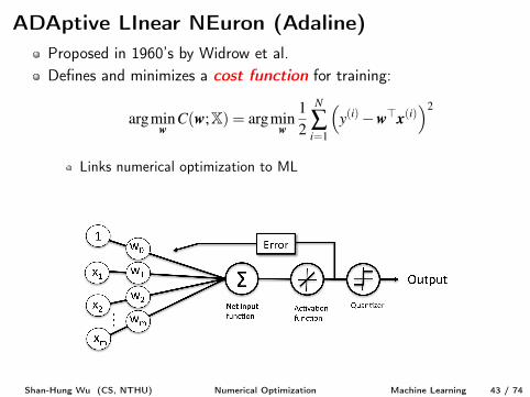
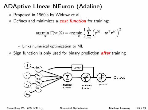
ADAptive LInear NEuron (Adaline)Proposed in 1960’s by Widrow et al.Defines and minimizes a cost function for training:
argmin
wC(w;X) = argmin
w
1
2
N
Âi=1
⇣y(i)�w>x(i)
⌘2
Links numerical optimization to ML
Sign function is only used for binary prediction after training
Shan-Hung Wu (CS, NTHU) Numerical Optimization Machine Learning 43 / 74
Training Using Gradient Descent
Update rule:
w(t+1) = w(t)�h—C(w(t))= w(t) +h Âi(y(i)�w(t)>x(i))x(i)
Since the cost function is convex, the training iterations will converge
Shan-Hung Wu (CS, NTHU) Numerical Optimization Machine Learning 44 / 74
Training Using Gradient Descent
Update rule:
w(t+1) = w(t)�h—C(w(t))= w(t) +h Âi(y(i)�w(t)>x(i))x(i)
Since the cost function is convex, the training iterations will converge
Shan-Hung Wu (CS, NTHU) Numerical Optimization Machine Learning 44 / 74
Outline1 Numerical Computation2 Optimization Problems3 Unconstrained Optimization
Gradient DescentNewton’s Method
4 Optimization in ML: Stochastic Gradient DescentPerceptronAdalineStochastic Gradient Descent
5 Constrained Optimization6 Optimization in ML: Regularization
Linear RegressionPolynomial RegressionGeneralizability & Regularization
7 Duality*
Shan-Hung Wu (CS, NTHU) Numerical Optimization Machine Learning 45 / 74
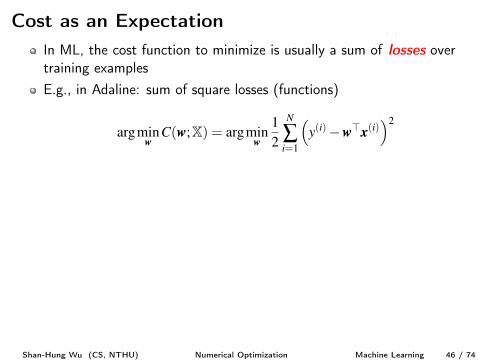
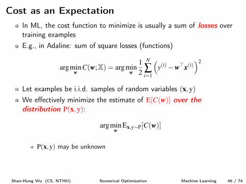
Cost as an ExpectationIn ML, the cost function to minimize is usually a sum of losses overtraining examplesE.g., in Adaline: sum of square losses (functions)
argmin
wC(w;X) = argmin
w
1
2
N
Âi=1
⇣y(i)�w>x(i)
⌘2
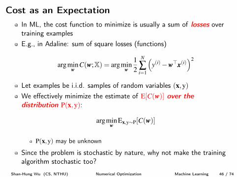
Let examples be i.i.d. samples of random variables (x,y)
We effectively minimize the estimate of E[C(w)] over the
distribution P(x,y):
argmin
wE
x,y⇠P
[C(w)]
P(x,y) may be unknown
Since the problem is stochastic by nature, why not make the trainingalgorithm stochastic too?
Shan-Hung Wu (CS, NTHU) Numerical Optimization Machine Learning 46 / 74
Cost as an ExpectationIn ML, the cost function to minimize is usually a sum of losses overtraining examplesE.g., in Adaline: sum of square losses (functions)
argmin
wC(w;X) = argmin
w
1
2
N
Âi=1
⇣y(i)�w>x(i)
⌘2
Let examples be i.i.d. samples of random variables (x,y)
We effectively minimize the estimate of E[C(w)] over the
distribution P(x,y):
argmin
wE
x,y⇠P
[C(w)]
P(x,y) may be unknown
Since the problem is stochastic by nature, why not make the trainingalgorithm stochastic too?
Shan-Hung Wu (CS, NTHU) Numerical Optimization Machine Learning 46 / 74
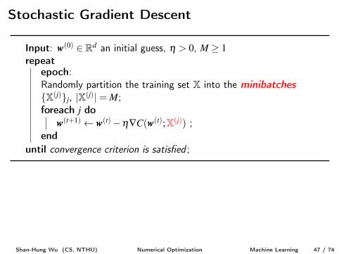
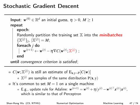
Stochastic Gradient Descent
Input: w(0) 2 Rd an initial guess, h > 0, M � 1
repeatepoch:Randomly partition the training set X into the minibatches
{X(j)}j, |X(j)|= M;foreach j do
w(t+1) w(t)�h—C(w(t);X(j)) ;
enduntil convergence criterion is satisfied ;
C(w;X(j)) is still an estimate of E
x,y⇠P
[C(w)]X(j) are samples of the same distribution P(x,y)
It’s common to set M = 1 on a single machineE.g., update rule for Adaline: w(t+1) = w(t) +h(y(t)�w(t)>x(t))x(t),which is similar to that of Perceptron
Shan-Hung Wu (CS, NTHU) Numerical Optimization Machine Learning 47 / 74
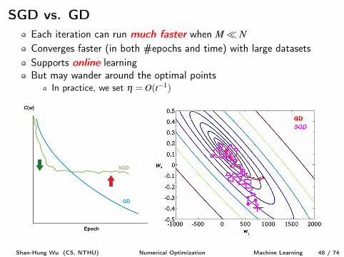
SGD vs. GDEach iteration can run much faster when M⌧ N
Converges faster (in both #epochs and time) with large datasetsSupports online learningBut may wander around the optimal points
In practice, we set h = O(t�1)
Shan-Hung Wu (CS, NTHU) Numerical Optimization Machine Learning 48 / 74
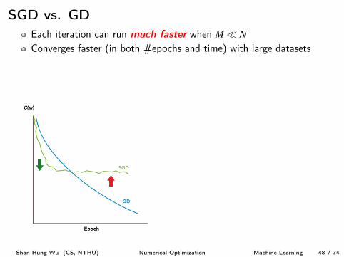
SGD vs. GDEach iteration can run much faster when M⌧ NConverges faster (in both #epochs and time) with large datasets
Supports online learningBut may wander around the optimal points
In practice, we set h = O(t�1)
Shan-Hung Wu (CS, NTHU) Numerical Optimization Machine Learning 48 / 74
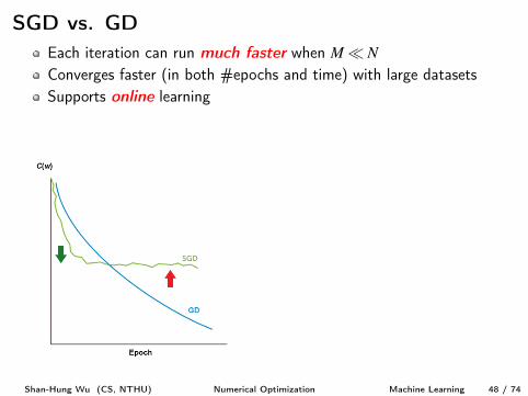
SGD vs. GDEach iteration can run much faster when M⌧ NConverges faster (in both #epochs and time) with large datasetsSupports online learning
But may wander around the optimal pointsIn practice, we set h = O(t�1)
Shan-Hung Wu (CS, NTHU) Numerical Optimization Machine Learning 48 / 74
SGD vs. GDEach iteration can run much faster when M⌧ NConverges faster (in both #epochs and time) with large datasetsSupports online learningBut may wander around the optimal points
In practice, we set h = O(t�1)
Shan-Hung Wu (CS, NTHU) Numerical Optimization Machine Learning 48 / 74
Outline1 Numerical Computation2 Optimization Problems3 Unconstrained Optimization
Gradient DescentNewton’s Method
4 Optimization in ML: Stochastic Gradient DescentPerceptronAdalineStochastic Gradient Descent
5 Constrained Optimization6 Optimization in ML: Regularization
Linear RegressionPolynomial RegressionGeneralizability & Regularization
7 Duality*
Shan-Hung Wu (CS, NTHU) Numerical Optimization Machine Learning 49 / 74
Constrained Optimization
Problem:minx f (x)
subject to x 2 C
f : Rd! R is not necessarily convexC= {x : g(i)(x) 0,h(j)(x) = 0}i,j
Iterative descent algorithm?
Shan-Hung Wu (CS, NTHU) Numerical Optimization Machine Learning 50 / 74
Constrained Optimization
Problem:minx f (x)
subject to x 2 C
f : Rd! R is not necessarily convexC= {x : g(i)(x) 0,h(j)(x) = 0}i,j
Iterative descent algorithm?
Shan-Hung Wu (CS, NTHU) Numerical Optimization Machine Learning 50 / 74
Common Methods
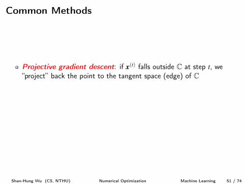
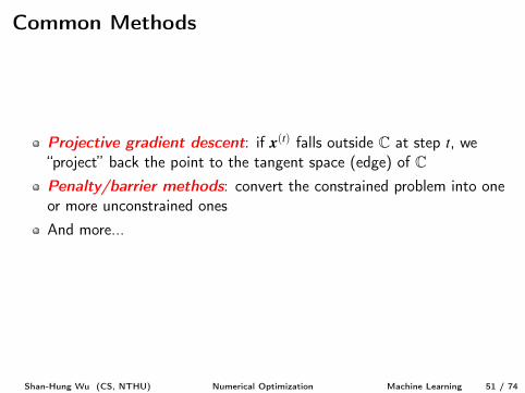
Projective gradient descent: if x(t) falls outside C at step t, we“project” back the point to the tangent space (edge) of C
Penalty/barrier methods: convert the constrained problem into oneor more unconstrained onesAnd more...
Shan-Hung Wu (CS, NTHU) Numerical Optimization Machine Learning 51 / 74
Common Methods
Projective gradient descent: if x(t) falls outside C at step t, we“project” back the point to the tangent space (edge) of CPenalty/barrier methods: convert the constrained problem into oneor more unconstrained onesAnd more...
Shan-Hung Wu (CS, NTHU) Numerical Optimization Machine Learning 51 / 74
Karush-Kuhn-Tucker (KKT) Methods I
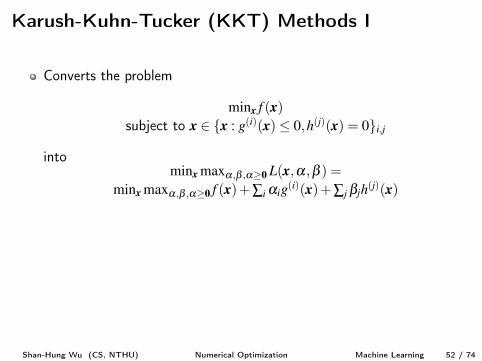
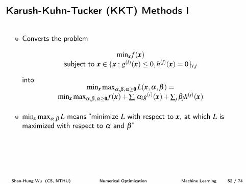
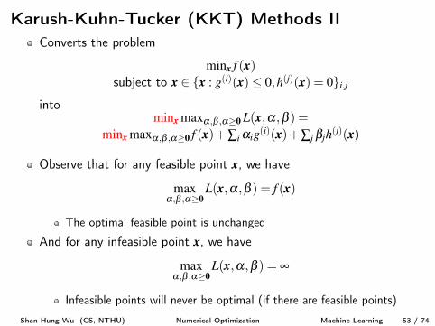
Converts the problem
minx f (x)subject to x 2 {x : g(i)(x) 0,h(j)(x) = 0}i,j
intominx maxa,b ,a�0
L(x,a,b ) =minx maxa,b ,a�0
f (x)+Âi aig(i)(x)+Âj bjh(j)(x)
minx maxa,b L means “minimize L with respect to x, at which L ismaximized with respect to a and b ”The function L(x,a,b ) is called the (generalized) Lagrangian
a and b are called KKT multipliers
Shan-Hung Wu (CS, NTHU) Numerical Optimization Machine Learning 52 / 74
Karush-Kuhn-Tucker (KKT) Methods I
Converts the problem
minx f (x)subject to x 2 {x : g(i)(x) 0,h(j)(x) = 0}i,j
intominx maxa,b ,a�0
L(x,a,b ) =minx maxa,b ,a�0
f (x)+Âi aig(i)(x)+Âj bjh(j)(x)
minx maxa,b L means “minimize L with respect to x, at which L ismaximized with respect to a and b ”
The function L(x,a,b ) is called the (generalized) Lagrangian
a and b are called KKT multipliers
Shan-Hung Wu (CS, NTHU) Numerical Optimization Machine Learning 52 / 74
Karush-Kuhn-Tucker (KKT) Methods I
Converts the problem
minx f (x)subject to x 2 {x : g(i)(x) 0,h(j)(x) = 0}i,j
intominx maxa,b ,a�0
L(x,a,b ) =minx maxa,b ,a�0
f (x)+Âi aig(i)(x)+Âj bjh(j)(x)
minx maxa,b L means “minimize L with respect to x, at which L ismaximized with respect to a and b ”The function L(x,a,b ) is called the (generalized) Lagrangian
a and b are called KKT multipliers
Shan-Hung Wu (CS, NTHU) Numerical Optimization Machine Learning 52 / 74
Karush-Kuhn-Tucker (KKT) Methods I
Converts the problem
minx f (x)subject to x 2 {x : g(i)(x) 0,h(j)(x) = 0}i,j
intominx maxa,b ,a�0
L(x,a,b ) =minx maxa,b ,a�0
f (x)+Âi aig(i)(x)+Âj bjh(j)(x)
minx maxa,b L means “minimize L with respect to x, at which L ismaximized with respect to a and b ”The function L(x,a,b ) is called the (generalized) Lagrangian
a and b are called KKT multipliers
Shan-Hung Wu (CS, NTHU) Numerical Optimization Machine Learning 52 / 74
Karush-Kuhn-Tucker (KKT) Methods IIConverts the problem
minx f (x)subject to x 2 {x : g(i)(x) 0,h(j)(x) = 0}i,j
intominx maxa,b ,a�0
L(x,a,b ) =minx maxa,b ,a�0
f (x)+Âi aig(i)(x)+Âj bjh(j)(x)
Observe that for any feasible point x, we have
max
a,b ,a�0
L(x,a,b ) = f (x)
The optimal feasible point is unchanged
And for any infeasible point x, we have
max
a,b ,a�0
L(x,a,b ) = •
Infeasible points will never be optimal (if there are feasible points)
Shan-Hung Wu (CS, NTHU) Numerical Optimization Machine Learning 53 / 74
Karush-Kuhn-Tucker (KKT) Methods IIConverts the problem
minx f (x)subject to x 2 {x : g(i)(x) 0,h(j)(x) = 0}i,j
intominx maxa,b ,a�0
L(x,a,b ) =minx maxa,b ,a�0
f (x)+Âi aig(i)(x)+Âj bjh(j)(x)
Observe that for any feasible point x, we have
max
a,b ,a�0
L(x,a,b ) = f (x)
The optimal feasible point is unchanged
And for any infeasible point x, we have
max
a,b ,a�0
L(x,a,b ) = •
Infeasible points will never be optimal (if there are feasible points)Shan-Hung Wu (CS, NTHU) Numerical Optimization Machine Learning 53 / 74
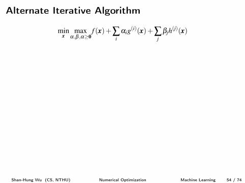
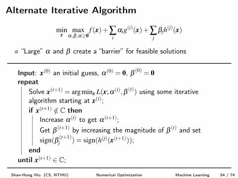
Alternate Iterative Algorithm
min
xmax
a,b ,a�0
f (x)+Âi
aig(i)(x)+Âj
bjh(j)(x)
“Large” a and b create a “barrier” for feasible solutions
Input: x(0) an initial guess, a(0) = 0, b (0) = 0
repeatSolve x(t+1) = argminx L(x;a(t),b (t)) using some iterativealgorithm starting at x(t);if x(t+1) /2 C then
Increase a(t) to get a(t+1);Get b (t+1) by increasing the magnitude of b (t) and setsign(b (t+1)
j ) = sign(h(j)(x(t+1)));end
until x(t+1) 2 C;
Shan-Hung Wu (CS, NTHU) Numerical Optimization Machine Learning 54 / 74

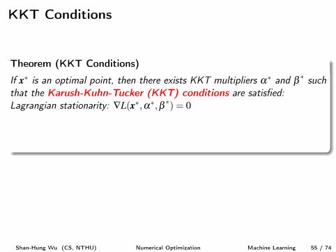
KKT Conditions
Theorem (KKT Conditions)
If x⇤ is an optimal point, then there exists KKT multipliers a⇤ and b ⇤ such
that the Karush-Kuhn-Tucker (KKT) conditions are satisfied:
Lagrangian stationarity: —L(x⇤,a⇤,b ⇤) = 0
Primal feasibility: g(i)(x⇤) 0 and h(j)(x⇤) = 0 for all i and jDual feasibility: a⇤ � 0
Complementary slackness: a⇤i g(i)(x⇤) = 0 for all i.
Only a necessary condition for x⇤ being optimalSufficient if the original problem is convex
Shan-Hung Wu (CS, NTHU) Numerical Optimization Machine Learning 55 / 74
KKT Conditions
Theorem (KKT Conditions)
If x⇤ is an optimal point, then there exists KKT multipliers a⇤ and b ⇤ such
that the Karush-Kuhn-Tucker (KKT) conditions are satisfied:
Lagrangian stationarity: —L(x⇤,a⇤,b ⇤) = 0
Primal feasibility: g(i)(x⇤) 0 and h(j)(x⇤) = 0 for all i and jDual feasibility: a⇤ � 0
Complementary slackness: a⇤i g(i)(x⇤) = 0 for all i.
Only a necessary condition for x⇤ being optimal
Sufficient if the original problem is convex
Shan-Hung Wu (CS, NTHU) Numerical Optimization Machine Learning 55 / 74
KKT Conditions
Theorem (KKT Conditions)
If x⇤ is an optimal point, then there exists KKT multipliers a⇤ and b ⇤ such
that the Karush-Kuhn-Tucker (KKT) conditions are satisfied:
Lagrangian stationarity: —L(x⇤,a⇤,b ⇤) = 0
Primal feasibility: g(i)(x⇤) 0 and h(j)(x⇤) = 0 for all i and jDual feasibility: a⇤ � 0
Complementary slackness: a⇤i g(i)(x⇤) = 0 for all i.
Only a necessary condition for x⇤ being optimalSufficient if the original problem is convex
Shan-Hung Wu (CS, NTHU) Numerical Optimization Machine Learning 55 / 74
Complementary Slackness
Why a⇤i g(i)(x⇤) = 0?For x⇤ being feasible, we have g(i)(x⇤) 0
If g(i) is active (i.e., g(i)(x⇤) = 0) then a⇤i g(i)(x⇤) = 0
If g(i) is inactive (i.e., g(i)(x⇤)< 0), thenTo maximize the aig(i)(x⇤) term in the Lagrangian in terms of aisubject to ai � 0, we have a⇤i = 0
Again a⇤i g(i)(x⇤) = 0
So what?a⇤i > 0 implies g(i)(x⇤) = 0
Once x⇤ is solved, we can quickly find out the active inequalityconstrains by checking a⇤i > 0
Shan-Hung Wu (CS, NTHU) Numerical Optimization Machine Learning 56 / 74
Complementary Slackness
Why a⇤i g(i)(x⇤) = 0?For x⇤ being feasible, we have g(i)(x⇤) 0
If g(i) is active (i.e., g(i)(x⇤) = 0) then a⇤i g(i)(x⇤) = 0
If g(i) is inactive (i.e., g(i)(x⇤)< 0), thenTo maximize the aig(i)(x⇤) term in the Lagrangian in terms of aisubject to ai � 0, we have a⇤i = 0
Again a⇤i g(i)(x⇤) = 0
So what?
a⇤i > 0 implies g(i)(x⇤) = 0
Once x⇤ is solved, we can quickly find out the active inequalityconstrains by checking a⇤i > 0
Shan-Hung Wu (CS, NTHU) Numerical Optimization Machine Learning 56 / 74
Complementary Slackness
Why a⇤i g(i)(x⇤) = 0?For x⇤ being feasible, we have g(i)(x⇤) 0
If g(i) is active (i.e., g(i)(x⇤) = 0) then a⇤i g(i)(x⇤) = 0
If g(i) is inactive (i.e., g(i)(x⇤)< 0), thenTo maximize the aig(i)(x⇤) term in the Lagrangian in terms of aisubject to ai � 0, we have a⇤i = 0
Again a⇤i g(i)(x⇤) = 0
So what?a⇤i > 0 implies g(i)(x⇤) = 0
Once x⇤ is solved, we can quickly find out the active inequalityconstrains by checking a⇤i > 0
Shan-Hung Wu (CS, NTHU) Numerical Optimization Machine Learning 56 / 74
Outline1 Numerical Computation2 Optimization Problems3 Unconstrained Optimization
Gradient DescentNewton’s Method
4 Optimization in ML: Stochastic Gradient DescentPerceptronAdalineStochastic Gradient Descent
5 Constrained Optimization6 Optimization in ML: Regularization
Linear RegressionPolynomial RegressionGeneralizability & Regularization
7 Duality*
Shan-Hung Wu (CS, NTHU) Numerical Optimization Machine Learning 57 / 74
Outline1 Numerical Computation2 Optimization Problems3 Unconstrained Optimization
Gradient DescentNewton’s Method
4 Optimization in ML: Stochastic Gradient DescentPerceptronAdalineStochastic Gradient Descent
5 Constrained Optimization6 Optimization in ML: Regularization
Linear RegressionPolynomial RegressionGeneralizability & Regularization
7 Duality*
Shan-Hung Wu (CS, NTHU) Numerical Optimization Machine Learning 58 / 74
The Regression Problem
Given a training dataset: X= {(x(i),y(i))}Ni=1
x(i) 2 RD, called explanatory variables (attributes/features)y(i) 2 R, called response/target variables (labels)
Goal: to find a function f (x) = y such that y is close to the true label y
Example: to predict the price of a stock tomorrowCould you define a model F= {f} and cost function C[f ]?How about “relaxing” the Adaline by removing the sign function whenmaking the final prediction?
Adaline: y = sign(w>x�b)Regressor: y = w>x�b
Shan-Hung Wu (CS, NTHU) Numerical Optimization Machine Learning 59 / 74
The Regression Problem
Given a training dataset: X= {(x(i),y(i))}Ni=1
x(i) 2 RD, called explanatory variables (attributes/features)y(i) 2 R, called response/target variables (labels)
Goal: to find a function f (x) = y such that y is close to the true label y
Example: to predict the price of a stock tomorrow
Could you define a model F= {f} and cost function C[f ]?How about “relaxing” the Adaline by removing the sign function whenmaking the final prediction?
Adaline: y = sign(w>x�b)Regressor: y = w>x�b
Shan-Hung Wu (CS, NTHU) Numerical Optimization Machine Learning 59 / 74
The Regression Problem
Given a training dataset: X= {(x(i),y(i))}Ni=1
x(i) 2 RD, called explanatory variables (attributes/features)y(i) 2 R, called response/target variables (labels)
Goal: to find a function f (x) = y such that y is close to the true label y
Example: to predict the price of a stock tomorrowCould you define a model F= {f} and cost function C[f ]?
How about “relaxing” the Adaline by removing the sign function whenmaking the final prediction?
Adaline: y = sign(w>x�b)Regressor: y = w>x�b
Shan-Hung Wu (CS, NTHU) Numerical Optimization Machine Learning 59 / 74
The Regression Problem
Given a training dataset: X= {(x(i),y(i))}Ni=1
x(i) 2 RD, called explanatory variables (attributes/features)y(i) 2 R, called response/target variables (labels)
Goal: to find a function f (x) = y such that y is close to the true label y
Example: to predict the price of a stock tomorrowCould you define a model F= {f} and cost function C[f ]?How about “relaxing” the Adaline by removing the sign function whenmaking the final prediction?
Adaline: y = sign(w>x�b)Regressor: y = w>x�b
Shan-Hung Wu (CS, NTHU) Numerical Optimization Machine Learning 59 / 74
Linear Regression I
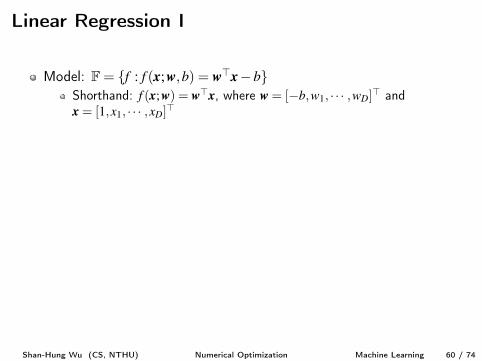
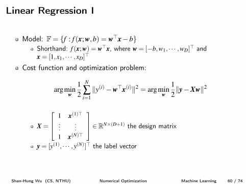
Model: F= {f : f (x;w,b) = w>x�b}Shorthand: f (x;w) = w>x, where w = [�b,w
1
, · · · ,wD]> andx = [1,x
1
, · · · ,xD]>
Cost function and optimization problem:
argmin
w
1
2
N
Âi=1
ky(i)�w>x(i)k2 = argmin
w
1
2
ky�Xwk2
X =
2
641 x(1)>...
...1 x(N)>
3
75 2 RN⇥(D+1) the design matrix
y = [y(1), · · · ,y(N)]> the label vector
Shan-Hung Wu (CS, NTHU) Numerical Optimization Machine Learning 60 / 74
Linear Regression I
Model: F= {f : f (x;w,b) = w>x�b}Shorthand: f (x;w) = w>x, where w = [�b,w
1
, · · · ,wD]> andx = [1,x
1
, · · · ,xD]>
Cost function and optimization problem:
argmin
w
1
2
N
Âi=1
ky(i)�w>x(i)k2 = argmin
w
1
2
ky�Xwk2
X =
2
641 x(1)>...
...1 x(N)>
3
75 2 RN⇥(D+1) the design matrix
y = [y(1), · · · ,y(N)]> the label vector
Shan-Hung Wu (CS, NTHU) Numerical Optimization Machine Learning 60 / 74
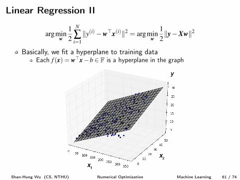
Linear Regression II
argmin
w
1
2
N
Âi=1
ky(i)�w>x(i)k2 = argmin
w
1
2
ky�Xwk2
Basically, we fit a hyperplane to training dataEach f (x) = w>x�b 2 F is a hyperplane in the graph
Shan-Hung Wu (CS, NTHU) Numerical Optimization Machine Learning 61 / 74
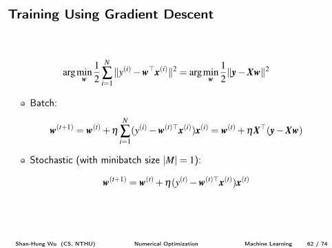
Training Using Gradient Descent
argmin
w
1
2
N
Âi=1
ky(i)�w>x(i)k2 = argmin
w
1
2
ky�Xwk2
Batch:
w(t+1) = w(t) +hN
Âi=1
(y(i)�w(t)>x(i))x(i) = w(t) +hX>(y�Xw)
Stochastic (with minibatch size |M|= 1):
w(t+1) = w(t) +h(y(t)�w(t)>x(t))x(t)
Shan-Hung Wu (CS, NTHU) Numerical Optimization Machine Learning 62 / 74
Evaluation Metrics of Regression Models
Given a training/testing set X= {(x(i),y(i))}Ni=1
How to evaluate the predictions y(i) made by a function f ?
Sum of Square Errors (SSE): ÂNi=1
(y(i)� y(i))2
Mean Square Error (MSE): 1
N ÂNi=1
(y(i)� y(i))2
Relative Square Error (RSE):
ÂNi=1
(y(i)� y(i))2
ÂNi=1
(y(i)� y(i))2
,
where y = 1
N Âi y(i)
What does it mean? Compares f with a dummy prediction y
Coefficient of Determination: R2 = 1�RSE 2 [0,1]Higher the better
Shan-Hung Wu (CS, NTHU) Numerical Optimization Machine Learning 63 / 74
Evaluation Metrics of Regression Models
Given a training/testing set X= {(x(i),y(i))}Ni=1
How to evaluate the predictions y(i) made by a function f ?Sum of Square Errors (SSE): ÂN
i=1
(y(i)� y(i))2
Mean Square Error (MSE): 1
N ÂNi=1
(y(i)� y(i))2
Relative Square Error (RSE):
ÂNi=1
(y(i)� y(i))2
ÂNi=1
(y(i)� y(i))2
,
where y = 1
N Âi y(i)
What does it mean?
Compares f with a dummy prediction y
Coefficient of Determination: R2 = 1�RSE 2 [0,1]Higher the better
Shan-Hung Wu (CS, NTHU) Numerical Optimization Machine Learning 63 / 74
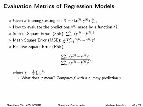
Evaluation Metrics of Regression Models
Given a training/testing set X= {(x(i),y(i))}Ni=1
How to evaluate the predictions y(i) made by a function f ?Sum of Square Errors (SSE): ÂN
i=1
(y(i)� y(i))2
Mean Square Error (MSE): 1
N ÂNi=1
(y(i)� y(i))2
Relative Square Error (RSE):
ÂNi=1
(y(i)� y(i))2
ÂNi=1
(y(i)� y(i))2
,
where y = 1
N Âi y(i)
What does it mean? Compares f with a dummy prediction y
Coefficient of Determination: R2 = 1�RSE 2 [0,1]Higher the better
Shan-Hung Wu (CS, NTHU) Numerical Optimization Machine Learning 63 / 74
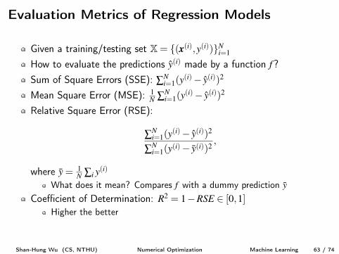
Outline1 Numerical Computation2 Optimization Problems3 Unconstrained Optimization
Gradient DescentNewton’s Method
4 Optimization in ML: Stochastic Gradient DescentPerceptronAdalineStochastic Gradient Descent
5 Constrained Optimization6 Optimization in ML: Regularization
Linear RegressionPolynomial RegressionGeneralizability & Regularization
7 Duality*
Shan-Hung Wu (CS, NTHU) Numerical Optimization Machine Learning 64 / 74
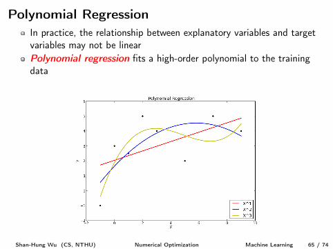
Polynomial RegressionIn practice, the relationship between explanatory variables and targetvariables may not be linearPolynomial regression fits a high-order polynomial to the trainingdata
How?
Shan-Hung Wu (CS, NTHU) Numerical Optimization Machine Learning 65 / 74
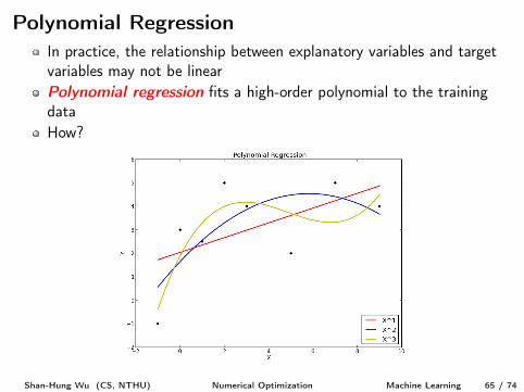
Polynomial RegressionIn practice, the relationship between explanatory variables and targetvariables may not be linearPolynomial regression fits a high-order polynomial to the trainingdataHow?
Shan-Hung Wu (CS, NTHU) Numerical Optimization Machine Learning 65 / 74
Data Augmentation
Suppose D = 2, i.e., x = [x1
,x2
]>
Linear model:
F= {f : f (x;w) = w>x+w0
= w0
+w1
x1
+w2
x2
}
Quadratic model:
F= {f : f (x;w) = w0
+w1
x1
+w2
x2
+w3
x2
1
+w4
x1
x2
+w5
x2
2
}
We can simply augment the data dimension to reduce a quadraticmodel to a linear one
A general technique in ML to “transform” a linear model into anonlinear one
How many variables to solve in w for a polynomial regression problemof degree P? [Homework]
Shan-Hung Wu (CS, NTHU) Numerical Optimization Machine Learning 66 / 74
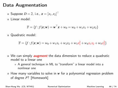
Outline1 Numerical Computation2 Optimization Problems3 Unconstrained Optimization
Gradient DescentNewton’s Method
4 Optimization in ML: Stochastic Gradient DescentPerceptronAdalineStochastic Gradient Descent
5 Constrained Optimization6 Optimization in ML: Regularization
Linear RegressionPolynomial RegressionGeneralizability & Regularization
7 Duality*
Shan-Hung Wu (CS, NTHU) Numerical Optimization Machine Learning 67 / 74
Regularization
There’s another major difference between the ML algorithms andoptimization techniques:
We usually care about the testing performance rather than thetraining performance
E.g., in classification, we report the testing accuracy
Goal: to learn a function that generalizes to unseen data wellRegularization: techniques that improve the generalizability of thelearned functionHow to regularize the linear regression?
argmin
w
1
2
ky�Xwk2
Shan-Hung Wu (CS, NTHU) Numerical Optimization Machine Learning 68 / 74
Regularization
There’s another major difference between the ML algorithms andoptimization techniques:We usually care about the testing performance rather than thetraining performance
E.g., in classification, we report the testing accuracy
Goal: to learn a function that generalizes to unseen data well
Regularization: techniques that improve the generalizability of thelearned functionHow to regularize the linear regression?
argmin
w
1
2
ky�Xwk2
Shan-Hung Wu (CS, NTHU) Numerical Optimization Machine Learning 68 / 74
Regularization
There’s another major difference between the ML algorithms andoptimization techniques:We usually care about the testing performance rather than thetraining performance
E.g., in classification, we report the testing accuracy
Goal: to learn a function that generalizes to unseen data wellRegularization: techniques that improve the generalizability of thelearned function
How to regularize the linear regression?
argmin
w
1
2
ky�Xwk2
Shan-Hung Wu (CS, NTHU) Numerical Optimization Machine Learning 68 / 74
Regularization
There’s another major difference between the ML algorithms andoptimization techniques:We usually care about the testing performance rather than thetraining performance
E.g., in classification, we report the testing accuracy
Goal: to learn a function that generalizes to unseen data wellRegularization: techniques that improve the generalizability of thelearned functionHow to regularize the linear regression?
argmin
w
1
2
ky�Xwk2
Shan-Hung Wu (CS, NTHU) Numerical Optimization Machine Learning 68 / 74
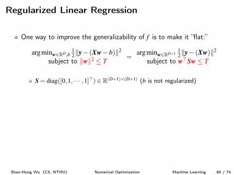
Regularized Linear Regression
One way to improve the generalizability of f is to make it “flat:”
argminw2RD,b1
2
ky� (Xw�b)k2
subject to kwk2 T=
argminw2RD+1
1
2
ky� (Xw)k2
subject to w>Sw T
S = diag([0,1, · · · ,1]>) 2 R(D+1)⇥(D+1) (b is not regularized)
We will explain why this works laterHow to solve this problem?Using the KKT method, we have
argmin
wmax
a,a�0
L(w,a) = argmin
wmax
a,a�0
1
2
⇣ky�Xwk2 +a(w>Sw�T)
⌘
Shan-Hung Wu (CS, NTHU) Numerical Optimization Machine Learning 69 / 74
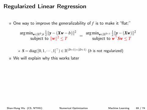
Regularized Linear Regression
One way to improve the generalizability of f is to make it “flat:”
argminw2RD,b1
2
ky� (Xw�b)k2
subject to kwk2 T=
argminw2RD+1
1
2
ky� (Xw)k2
subject to w>Sw T
S = diag([0,1, · · · ,1]>) 2 R(D+1)⇥(D+1) (b is not regularized)
We will explain why this works later
How to solve this problem?Using the KKT method, we have
argmin
wmax
a,a�0
L(w,a) = argmin
wmax
a,a�0
1
2
⇣ky�Xwk2 +a(w>Sw�T)
⌘
Shan-Hung Wu (CS, NTHU) Numerical Optimization Machine Learning 69 / 74
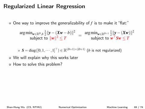
Regularized Linear Regression
One way to improve the generalizability of f is to make it “flat:”
argminw2RD,b1
2
ky� (Xw�b)k2
subject to kwk2 T=
argminw2RD+1
1
2
ky� (Xw)k2
subject to w>Sw T
S = diag([0,1, · · · ,1]>) 2 R(D+1)⇥(D+1) (b is not regularized)
We will explain why this works laterHow to solve this problem?
Using the KKT method, we have
argmin
wmax
a,a�0
L(w,a) = argmin
wmax
a,a�0
1
2
⇣ky�Xwk2 +a(w>Sw�T)
⌘
Shan-Hung Wu (CS, NTHU) Numerical Optimization Machine Learning 69 / 74
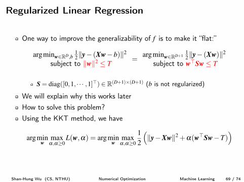
Regularized Linear Regression
One way to improve the generalizability of f is to make it “flat:”
argminw2RD,b1
2
ky� (Xw�b)k2
subject to kwk2 T=
argminw2RD+1
1
2
ky� (Xw)k2
subject to w>Sw T
S = diag([0,1, · · · ,1]>) 2 R(D+1)⇥(D+1) (b is not regularized)
We will explain why this works laterHow to solve this problem?Using the KKT method, we have
argmin
wmax
a,a�0
L(w,a) = argmin
wmax
a,a�0
1
2
⇣ky�Xwk2 +a(w>Sw�T)
⌘
Shan-Hung Wu (CS, NTHU) Numerical Optimization Machine Learning 69 / 74
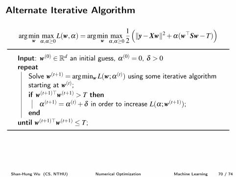
Alternate Iterative Algorithm
argmin
wmax
a,a�0
L(w,a) = argmin
wmax
a,a�0
1
2
⇣ky�Xwk2 +a(w>Sw�T)
⌘
Input: w(0) 2 Rd an initial guess, a(0) = 0, d > 0
repeatSolve w(t+1) = argminw L(w;a(t)) using some iterative algorithmstarting at w(t);if w(t+1)>w(t+1) > T then
a(t+1) = a(t) +d in order to increase L(a;w(t+1));end
until w(t+1)>w(t+1) T;
We could also solve w(t+1) analytically from ∂∂x L(w;a(t)) = 0:
w(t+1) =⇣
X>X+a(t)S⌘�1
X>y
Shan-Hung Wu (CS, NTHU) Numerical Optimization Machine Learning 70 / 74
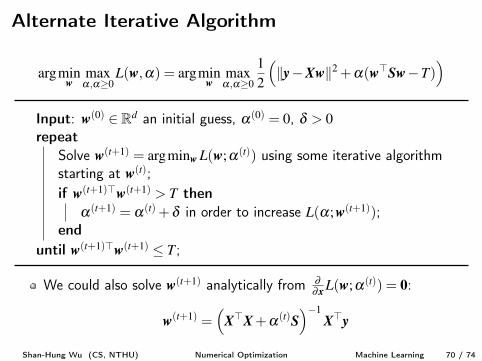
Outline1 Numerical Computation2 Optimization Problems3 Unconstrained Optimization
Gradient DescentNewton’s Method
4 Optimization in ML: Stochastic Gradient DescentPerceptronAdalineStochastic Gradient Descent
5 Constrained Optimization6 Optimization in ML: Regularization
Linear RegressionPolynomial RegressionGeneralizability & Regularization
7 Duality*
Shan-Hung Wu (CS, NTHU) Numerical Optimization Machine Learning 71 / 74
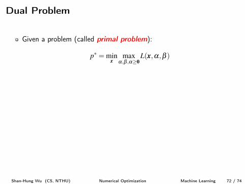
Dual Problem
Given a problem (called primal problem):
p⇤ = min
xmax
a,b ,a�0
L(x,a,b )
We define its dual problem as:
d⇤ = max
a,b ,a�0
min
xL(x,a,b )
By the max-min inequality, we have d⇤ p⇤ [Homework](p⇤ �d⇤) is called the duality gap
p⇤ and d⇤ are called the primal and dual values, respectively
Shan-Hung Wu (CS, NTHU) Numerical Optimization Machine Learning 72 / 74
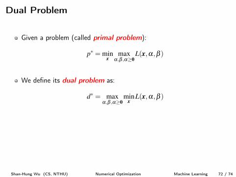
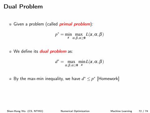
Dual Problem
Given a problem (called primal problem):
p⇤ = min
xmax
a,b ,a�0
L(x,a,b )
We define its dual problem as:
d⇤ = max
a,b ,a�0
min
xL(x,a,b )
By the max-min inequality, we have d⇤ p⇤ [Homework]
(p⇤ �d⇤) is called the duality gap
p⇤ and d⇤ are called the primal and dual values, respectively
Shan-Hung Wu (CS, NTHU) Numerical Optimization Machine Learning 72 / 74
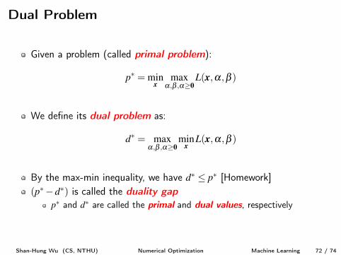
Dual Problem
Given a problem (called primal problem):
p⇤ = min
xmax
a,b ,a�0
L(x,a,b )
We define its dual problem as:
d⇤ = max
a,b ,a�0
min
xL(x,a,b )
By the max-min inequality, we have d⇤ p⇤ [Homework](p⇤ �d⇤) is called the duality gap
p⇤ and d⇤ are called the primal and dual values, respectively
Shan-Hung Wu (CS, NTHU) Numerical Optimization Machine Learning 72 / 74
Strong Duality
Strong duality holds if d⇤ = p⇤
When will it happen?
If the primal problem has solution and convex
Why considering dual problem?
Shan-Hung Wu (CS, NTHU) Numerical Optimization Machine Learning 73 / 74
Strong Duality
Strong duality holds if d⇤ = p⇤
When will it happen?If the primal problem has solution and convex
Why considering dual problem?
Shan-Hung Wu (CS, NTHU) Numerical Optimization Machine Learning 73 / 74
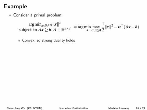
ExampleConsider a primal problem:
argminx2Rd1
2
kxk2
subject to Ax� b, A 2 Rn⇥d = argmin
xmax
a,a�0
1
2
kxk2�a>(Ax�b)
Convex, so strong duality holds
We can get the same solution via the dual problem:
arg max
a,a�0
min
x
1
2
kxk2�a>(Ax�b)
Solving minx L(x,a) analytically, we have x⇤ = A>aSubstituting this into the dual, we get
arg max
a,a�0
�1
2
kA>ak2 +b>a
We now solve n variables instead of d (beneficial when n⌧ d)
Shan-Hung Wu (CS, NTHU) Numerical Optimization Machine Learning 74 / 74
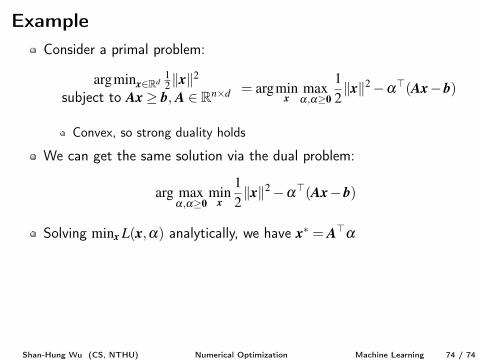
ExampleConsider a primal problem:
argminx2Rd1
2
kxk2
subject to Ax� b, A 2 Rn⇥d = argmin
xmax
a,a�0
1
2
kxk2�a>(Ax�b)
Convex, so strong duality holds
We can get the same solution via the dual problem:
arg max
a,a�0
min
x
1
2
kxk2�a>(Ax�b)
Solving minx L(x,a) analytically, we have x⇤ = A>a
Substituting this into the dual, we get
arg max
a,a�0
�1
2
kA>ak2 +b>a
We now solve n variables instead of d (beneficial when n⌧ d)
Shan-Hung Wu (CS, NTHU) Numerical Optimization Machine Learning 74 / 74
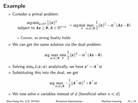
ExampleConsider a primal problem:
argminx2Rd1
2
kxk2
subject to Ax� b, A 2 Rn⇥d = argmin
xmax
a,a�0
1
2
kxk2�a>(Ax�b)
Convex, so strong duality holds
We can get the same solution via the dual problem:
arg max
a,a�0
min
x
1
2
kxk2�a>(Ax�b)
Solving minx L(x,a) analytically, we have x⇤ = A>aSubstituting this into the dual, we get
arg max
a,a�0
�1
2
kA>ak2 +b>a
We now solve n variables instead of d (beneficial when n⌧ d)
Shan-Hung Wu (CS, NTHU) Numerical Optimization Machine Learning 74 / 74
Recommended