Fundamentals of Power Electronics Chapter 13: Basic Magnetics Theory1
Part III. Magnetics
13 Basic Magnetics Theory
14 Inductor Design
15 Transformer Design

Fundamentals of Power Electronics Chapter 13: Basic Magnetics Theory2
Chapter 13 Basic Magnetics Theory
13.1 Review of Basic Magnetics
13.1.1 Basic relationships 13.1.2 Magnetic circuits
13.2 Transformer Modeling
13.2.1 The ideal transformer 13.2.3 Leakage inductances
13.2.2 The magnetizing inductance
13.3 Loss Mechanisms in Magnetic Devices
13.3.1 Core loss 13.3.2 Low-frequency copper loss
13.4 Eddy Currents in Winding Conductors
13.4.1 Skin and proximity effects 13.4.4 Power loss in a layer
13.4.2 Leakage flux in windings 13.4.5 Example: power loss in a
transformer winding
13.4.3 Foil windings and layers 13.4.6 Interleaving the windings
13.4.7 PWM waveform harmonics

Fundamentals of Power Electronics Chapter 13: Basic Magnetics Theory3
Chapter 13 Basic Magnetics Theory
13.5 Several Types of Magnetic Devices, Their B–H Loops, and Core vs.
Copper Loss
13.5.1 Filter inductor 13.5.4 Coupled inductor
13.5.2 AC inductor 13.5.5 Flyback transformer
13.5.3 Transformer
13.6 Summary of Key Points

Fundamentals of Power Electronics Chapter 13: Basic Magnetics Theory4
13.1 Review of Basic Magnetics13.1.1 Basic relationships
v(t)
i(t)
B(t), Φ(t)
H(t), F(t)
Terminalcharacteristics
Corecharacteristics
Faraday’s law
Ampere’s law

Fundamentals of Power Electronics Chapter 13: Basic Magnetics Theory5
Basic quantities
Electric field E
VoltageV = El
Total flux Φ
Flux density B {Surface Swith area Ac
Total current I
Current density J {Surface Swith area Ac
Length l Length l
Magnetic quantities Electrical quantities
Magnetic field H
+ –x1 x2
MMFF = Hl
+ –x1 x2

Fundamentals of Power Electronics Chapter 13: Basic Magnetics Theory6
Magnetic field H and magnetomotive force F
Example: uniform magnetic
field of magnitude H
Magnetomotive force (MMF) F between points x1 and x2 is related to
the magnetic field H according to
Analogous to electric field of
strength E, which induces
voltage (EMF) V:
F = H ⋅⋅dllx1
x2
Length l
Magnetic field H
+ –x1 x2
MMFF = Hl
Electric field E
VoltageV = El
Length l
+ –x1 x2

Fundamentals of Power Electronics Chapter 13: Basic Magnetics Theory7
Flux density B and total flux
Example: uniform flux density of
magnitude B
The total magnetic flux passing through a surface of area Ac is
related to the flux density B according to
Analogous to electrical conductor
current density of magnitude J,
which leads to total conductor
current I:
Φ = B ⋅⋅dAsurface S
Total flux Φ
Flux density B {Surface Swith area Ac
Total current I
Current density J {Surface Swith area Ac

Fundamentals of Power Electronics Chapter 13: Basic Magnetics Theory8
Faraday’s law
Voltage v(t) is induced in a
loop of wire by change inthe total flux (t) passing
through the interior of the
loop, according to
For uniform flux distribution,(t) = B(t)Ac and hence
{Area Ac
Flux Φ(t)
v(t)+
–
v(t) =dΦ(t)
dt
v(t) = AcdB(t)
dt

Fundamentals of Power Electronics Chapter 13: Basic Magnetics Theory9
Lenz’s law
The voltage v(t) induced by the changing flux (t) is of the polarity that
tends to drive a current through the loop to counteract the flux change.
Example: a shorted loop of wire
• Changing flux (t) induces a
voltage v(t) around the loop
• This voltage, divided by the
impedance of the loopconductor, leads to current i(t)
• This current induces a flux(t), which tends to oppose
changes in (t)
Flux Φ(t)
Induced currenti(t)
Shortedloop
Inducedflux Φ′(t)

Fundamentals of Power Electronics Chapter 13: Basic Magnetics Theory10
Ampere’s law
The net MMF around a closed path is equal to the total current
passing through the interior of the path:
Example: magnetic core. Wire
carrying current i(t) passes
through core window.
• Illustrated path follows
magnetic flux lines
around interior of core
• For uniform magnetic field
strength H(t), the integral (MMF)
is H(t)lm. So
H ⋅⋅dllclosed path
= total current passing through interior of path
i(t)
H
Magnetic pathlength lm
F(t) = H(t)lm = i(t)

Fundamentals of Power Electronics Chapter 13: Basic Magnetics Theory11
Ampere’s law: discussion
• Relates magnetic field strength H(t) to winding current i(t)
• We can view winding currents as sources of MMF
• Previous example: total MMF around core, F(t) = H(t)lm, is equal to
the winding current MMF i(t)
• The total MMF around a closed loop, accounting for winding current
MMF’s, is zero

Fundamentals of Power Electronics Chapter 13: Basic Magnetics Theory12
Core material characteristics:the relation between B and H
Free space A magnetic core material
0 = permeability of free space
= 4 · 10–7 Henries per meter
Highly nonlinear, with hysteresis
and saturation
B
Hµ0
B
H
µ
B = µ0H

Fundamentals of Power Electronics Chapter 13: Basic Magnetics Theory13
Piecewise-linear modelingof core material characteristics
No hysteresis or saturation Saturation, no hysteresis
Typical r = 103 to 105 Typical Bsat = 0.3 to 0.5T, ferrite
0.5 to 1T, powdered iron
1 to 2T, iron laminations
B
H
µ = µr µ0
B
H
µ
Bsat
– Bsat
B = µHµ = µrµ0

Fundamentals of Power Electronics Chapter 13: Basic Magnetics Theory14
Units
Table 12.1. Units for magnetic quantities
quantity MKS unrationalized cgs conversions
core material equation B = µ0 µr H B = µr H
B Tesla Gauss 1T = 104G
H Ampere / meter Oersted 1A/m = 4π 10-3
Oe
Weber Maxwell 1Wb = 108 Mx
1T = 1Wb / m2

Fundamentals of Power Electronics Chapter 13: Basic Magnetics Theory15
Example: a simple inductor
Faraday’s law:
For each turn of
wire, we can write
Total winding voltage is
Express in terms of the average flux density B(t) = F(t)/Ac
core
nturns
Core areaAc
Corepermeabilityµ
+v(t)–
i(t)Φ
vturn(t) =dΦ(t)
dt
v(t) = nvturn(t) = ndΦ(t)
dt
v(t) = nAcdB(t)
dt

Fundamentals of Power Electronics Chapter 13: Basic Magnetics Theory16
Inductor example: Ampere’s law
Choose a closed path
which follows the average
magnetic field line around
the interior of the core.
Length of this path is
called the mean magnetic
path length lm.
For uniform field strength
H(t), the core MMF
around the path is H lm.
Winding contains n turns of wire, each carrying current i(t). The net current
passing through the path interior (i.e., through the core window) is ni(t).
From Ampere’s law, we have
H(t) lm = n i(t)
nturns
i(t)
H
Magneticpathlength lm

Fundamentals of Power Electronics Chapter 13: Basic Magnetics Theory17
Inductor example: core material model
Find winding current at onset of saturation:
substitute i = Isat and H = Bsat / into
equation previously derived via Ampere’s
law. Result is
B =
Bsat for H ≥ Bsat/µ
µH for H < Bsat/µ
– Bsat for H ≤ – Bsat/µ
B
H
µ
Bsat
– Bsat
I sat =Bsatlm
µn

Fundamentals of Power Electronics Chapter 13: Basic Magnetics Theory18
Electrical terminal characteristics
We have:
H(t) lm = n i(t)
Eliminate B and H, and solve for relation between v and i. For | i | < Isat,
which is of the form
with
—an inductor
For | i | > Isat the flux density is constant and equal to Bsat. Faraday’s
law then predicts
—saturation leads to short circuit
v(t) = Ldi(t)dt L =
µn2Ac
lm
v(t) = nAcdBsat
dt= 0
v(t) = µnAcdH(t)
dt
B =
Bsat for H ≥ Bsat/µ
µH for H < Bsat/µ
– Bsat for H ≤ – Bsat/µ
v(t) = nAcdB(t)
dt
v(t) =µn2Ac
lm
di(t)dt

Fundamentals of Power Electronics Chapter 13: Basic Magnetics Theory19
13.1.2 Magnetic circuits
Uniform flux and
magnetic field inside
a rectangular
element:
MMF between ends of
element is
Since H = B / and = / Ac, we can express F as
with
A corresponding model:
R = reluctance of element
FluxΦ {
Length lMMF F Area
Ac
Core permeability µ
H
+ –
R = l
µAcF = Hl
F = ΦRR = l
µAc
Φ
F+ –
R

Fundamentals of Power Electronics Chapter 13: Basic Magnetics Theory20
Magnetic circuits: magnetic structures composed ofmultiple windings and heterogeneous elements
• Represent each element with reluctance
• Windings are sources of MMF
• MMF voltage, flux current
• Solve magnetic circuit using Kirchoff’s laws, etc.

Fundamentals of Power Electronics Chapter 13: Basic Magnetics Theory21
Magnetic analog of Kirchoff’s current law
Divergence of B = 0
Flux lines are continuous
and cannot end
Total flux entering a node
must be zero
Physical structure
Magnetic circuit
Φ1
Φ2
Φ3
Node
Φ1
Φ2
Φ3
Node Φ1 = Φ2 + Φ3

Fundamentals of Power Electronics Chapter 13: Basic Magnetics Theory22
Magnetic analog of Kirchoff’s voltage law
Follows from Ampere’s law:
Left-hand side: sum of MMF’s across the reluctances around the
closed path
Right-hand side: currents in windings are sources of MMF’s. An n-turn
winding carrying current i(t) is modeled as an MMF (voltage) source,
of value ni(t).
Total MMF’s around the closed path add up to zero.
H ⋅⋅dllclosed path
= total current passing through interior of path

Fundamentals of Power Electronics Chapter 13: Basic Magnetics Theory23
Example: inductor with air gap
+v(t)–
Air gaplg
nturns
Cross-sectionalarea Ac
i(t)
Φ
Magnetic pathlength lm
Corepermeability µ

Fundamentals of Power Electronics Chapter 13: Basic Magnetics Theory24
Magnetic circuit model
+v(t)–
Air gaplg
nturns
Cross-sectionalarea Ac
i(t)
Φ
Magnetic pathlength lm
Corepermeability µ
+–ni(t) Φ(t)
Rc
Rg
Fc
Fg
+ –
+
–
Fc + Fg = ni Rc =lc
µAc
Rg =lg
µ0Acni = Φ Rc + Rg

Fundamentals of Power Electronics Chapter 13: Basic Magnetics Theory25
Solution of model
Faraday’s law:
Substitute for :
Hence inductance is
+v(t)–
Air gaplg
nturns
Cross-sectionalarea Ac
i(t)
Φ
Magnetic pathlength lm
Corepermeability µ
+–ni(t) Φ(t)
Rc
Rg
Fc
Fg
+ –
+
–
Rc =lc
µAc
Rg =lg
µ0Ac
ni = Φ Rc + Rgv(t) = ndΦ(t)
dt
v(t) = n2
Rc + Rg
di(t)dt
L = n2
Rc + Rg
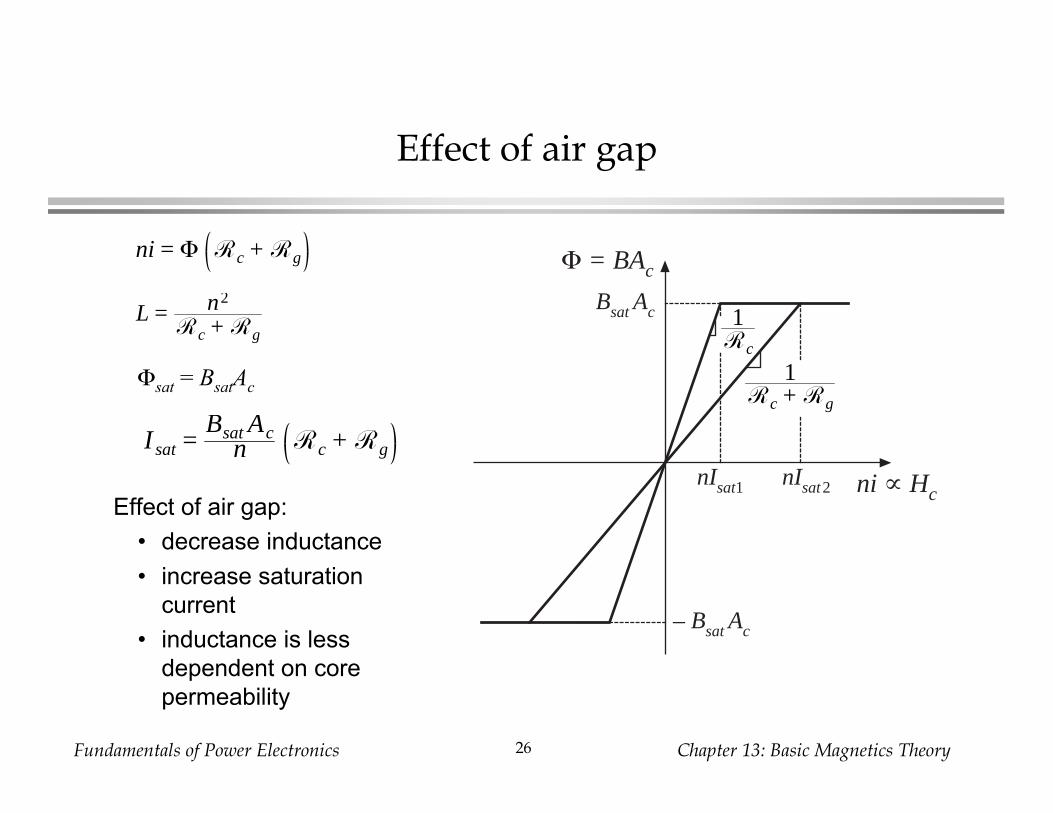
Fundamentals of Power Electronics Chapter 13: Basic Magnetics Theory26
Effect of air gap
Effect of air gap:
• decrease inductance
• increase saturation
current
• inductance is less
dependent on core
permeability
sat = BsatAc1
Rc + Rg
1Rc
Φ = BAc
ni ∝ Hc
Bsat Ac
– Bsat Ac
nIsat1 nIsat2
ni = Φ Rc + Rg
L = n2
Rc + Rg
I sat =Bsat Ac
n Rc + Rg

Fundamentals of Power Electronics Chapter 13: Basic Magnetics Theory27
13.2 Transformer modeling
Two windings, no air gap:
Magnetic circuit model:
Core
Φ
n1turns
+v1(t)
–
i1(t)
+v2(t)
–
i2(t)
n2turns
R =lm
µAc
Fc = n1i1 + n2i2
ΦR = n1i1 + n2i2
+–n1i1
ΦRc
Fc+ –
+–
n2i2

Fundamentals of Power Electronics Chapter 13: Basic Magnetics Theory28
13.2.1 The ideal transformer
In the ideal transformer, the core
reluctance R approaches zero.
MMF Fc = R also approaches
zero. We then obtain
Also, by Faraday’s law,
Eliminate :
Ideal transformer equations:
+–n1i1
ΦRc
Fc+ –
+–
n2i2
Ideal
n1 : n2
+
v1
–
+
v2
–
i1 i2
0 = n1i1 + n2i2
v1 = n1dΦdt
v2 = n2dΦdt
dΦdt
=v1
n1
=v2
n2
v1
n1
=v2
n2
and n1i1 + n2i2 = 0
Fundamentals of Power Electronics Chapter 13: Basic Magnetics Theory29
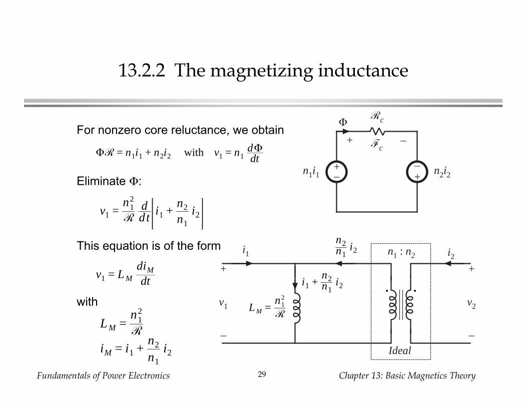
13.2.2 The magnetizing inductance
For nonzero core reluctance, we obtain
Eliminate :
This equation is of the form
with
+–n1i1
ΦRc
Fc+ –
+–
n2i2
Ideal
n1 : n2
+
v1
–
+
v2
–
i1 i2
n2n1
i2
i1 +n2n1
i2
L M =n1
2
R
ΦR = n1i1 + n2i2 with v1 = n1dΦdt
v1 =n1
2
R
ddt
i1 +n2
n1
i2
v1 = L M
diM
dt
L M =n1
2
R
iM = i1 +n2
n1
i2

Fundamentals of Power Electronics Chapter 13: Basic Magnetics Theory30
Magnetizing inductance: discussion
• Models magnetization of core material
• A real, physical inductor, that exhibits saturation and hysteresis
• If the secondary winding is disconnected:
we are left with the primary winding on the core
primary winding then behaves as an inductor
the resulting inductor is the magnetizing inductance, referred to
the primary winding
• Magnetizing current causes the ratio of winding currents to differ
from the turns ratio

Fundamentals of Power Electronics Chapter 13: Basic Magnetics Theory31
Transformer saturation
• Saturation occurs when core flux density B(t) exceeds saturation
flux density Bsat.
• When core saturates, the magnetizing current becomes large, the
impedance of the magnetizing inductance becomes small, and the
windings are effectively shorted out.
• Large winding currents i1(t) and i2(t) do not necessarily lead to
saturation. If
then the magnetizing current is zero, and there is no net
magnetization of the core.
• Saturation is caused by excessive applied volt-seconds
0 = n1i1 + n2i2

Fundamentals of Power Electronics Chapter 13: Basic Magnetics Theory32
Saturation vs. applied volt-seconds
Magnetizing current
depends on the integral
of the applied winding
voltage:
Flux density is
proportional:
Flux density becomes large, and coresaturates, when the applied volt-seconds 1
are too large, where
limits of integration chosen to coincide with
positive portion of applied voltage waveform
Ideal
n1 : n2
+
v1
–
+
v2
–
i1 i2
n2n1
i2
i1 +n2n1
i2
L M =n1
2
R
iM(t) = 1L M
v1(t)dt
B(t) = 1n1Ac
v1(t)dt
λ1 = v1(t)dtt1
t2

Fundamentals of Power Electronics Chapter 13: Basic Magnetics Theory33
13.2.3 Leakage inductances
ΦM
+v1(t)
–
i1(t)
+v2(t)
–
i2(t)
Φl1 Φ
l2
ΦM
+v1(t)
–
i1(t)
+v2(t)
–
i2(t)
Φl2Φ
l1

Fundamentals of Power Electronics Chapter 13: Basic Magnetics Theory34
Transformer model, including leakage inductance
effective turns ratio
coupling coefficient
mutual inductance:
primary and secondary
self-inductances:
Ideal
n1 : n2
+
v1
–
+
v2
–
i1 i2Ll1 L
l2
L M =n1n2
L 12
iMv1(t)v2(t)
=L11 L12L12 L22
ddt
i1(t)i2(t)
Terminal equations can
be written in the form
L12 =n1n2
R
=n2n1
L M
L11 = Ll1 +
n1n2
L12
L22 = Ll2 +
n2n1
L12
ne =L22L11
k =L12
L11L22

Fundamentals of Power Electronics Chapter 13: Basic Magnetics Theory35
13.3 Loss mechanisms in magnetic devices
Low-frequency losses:
Dc copper loss
Core loss: hysteresis loss
High-frequency losses: the skin effect
Core loss: classical eddy current losses
Eddy current losses in ferrite cores
High frequency copper loss: the proximity effect
Proximity effect: high frequency limit
MMF diagrams, losses in a layer, and losses in basic multilayer
windings
Effect of PWM waveform harmonics

Fundamentals of Power Electronics Chapter 13: Basic Magnetics Theory36
13.3.1 Core loss
Energy per cycle W flowing into n-
turn winding of an inductor,
excited by periodic waveforms of
frequency f:
Relate winding voltage and current to core B
and H via Faraday’s law and Ampere’s law:
H(t)lm = ni(t)
Substitute into integral:
core
nturns
Core areaAc
Corepermeabilityµ
+v(t)–
i(t)Φ
W = v(t)i(t)dtone cycle
v(t) = nAcdB(t)
dt
W = nAcdB(t)
dtH(t)lm
n dt
one cycle
= Aclm H dBone cycle

Fundamentals of Power Electronics Chapter 13: Basic Magnetics Theory37
Core loss: Hysteresis loss
(energy lost per cycle) = (core volume) (area of B–H loop)
The term Aclm is the volume of
the core, while the integral is
the area of the B–H loop.
Hysteresis loss is directly proportional
to applied frequency
B
H
Area
H dBone cycle
W = Aclm H dBone cycle
PH = f Aclm H dBone cycle

Fundamentals of Power Electronics Chapter 13: Basic Magnetics Theory38
Modeling hysteresis loss
• Hysteresis loss varies directly with applied frequency
• Dependence on maximum flux density: how does area of B–H loop
depend on maximum flux density (and on applied waveforms)?
Empirical equation (Steinmetz equation):
The parameters KH and are determined experimentally.
Dependence of PH on Bmax is predicted by the theory of magnetic
domains.
PH = KH f Bmaxα (core volume)

Fundamentals of Power Electronics Chapter 13: Basic Magnetics Theory39
Core loss: eddy current loss
Magnetic core materials are reasonably good conductors of electric
current. Hence, according to Lenz’s law, magnetic fields within the
core induce currents (“eddy currents”) to flow within the core. The
eddy currents flow such that they tend to generate a flux whichopposes changes in the core flux (t). The eddy currents tend to
prevent flux from penetrating the core.
Eddy current
loss i2(t)RFluxΦ(t)
Core
i(t)
Eddycurrent

Fundamentals of Power Electronics Chapter 13: Basic Magnetics Theory40
Modeling eddy current loss
• Ac flux (t) induces voltage v(t) in core, according to Faraday’s law.
Induced voltage is proportional to derivative of (t). In
consequence, magnitude of induced voltage is directly proportional
to excitation frequency f.
• If core material impedance Z is purely resistive and independent of
frequency, Z = R, then eddy current magnitude is proportional to
voltage: i(t) = v(t)/R. Hence magnitude of i(t) is directly proportional
to excitation frequency f.
• Eddy current power loss i2(t)R then varies with square of excitation
frequency f.
• Classical Steinmetz equation for eddy current loss:
• Ferrite core material impedance is capacitive. This causes eddy
current power loss to increase as f 4.
PE = KE f 2Bmax2 (core volume)

Fundamentals of Power Electronics Chapter 13: Basic Magnetics Theory41
Total core loss: manufacturer’s data
Empirical equation, at a
fixed frequency:
Ferrite core
material
∆B, Tesla
0.01 0.1 0.3
Pow
er lo
ss d
ensi
ty, W
atts
/cm
3
0.01
0.1
1
20kH
z50
kHz
100k
Hz
200k
Hz
500k
Hz
1MH
z
Pfe = K fe (∆B)β Ac lm

Fundamentals of Power Electronics Chapter 13: Basic Magnetics Theory42
Core materials
Core type Bsat
Relative core loss Applications
Laminationsiron, silicon steel
1.5 - 2.0 T high 50-60 Hz transformers,inductors
Powdered corespowdered iron,molypermalloy
0.6 - 0.8 T medium 1 kHz transformers,100 kHz filter inductors
FerriteManganese-zinc,Nickel-zinc
0.25 - 0.5 T low 20 kHz - 1 MHztransformers,ac inductors

Fundamentals of Power Electronics Chapter 13: Basic Magnetics Theory43
13.3.2 Low-frequency copper loss
DC resistance of wire
where Aw is the wire bare cross-sectional area, and
lb is the length of the wire. The resistivity is equal
to 1.724 10–6 cm for soft-annealed copper at room
temperature. This resistivity increases to2.3 10–6 cm at 100˚C.
The wire resistance leads to a power loss of
R
i(t)
R = ρlb
Aw
Pcu = I rms2 R

Fundamentals of Power Electronics Chapter 13: Basic Magnetics Theory44
13.4 Eddy currents in winding conductors13.4.1 Intro to the skin and proximity effects
i(t)
Wire
Φ(t)
Eddycurrents
i(t)
Wire
Eddycurrents
Currentdensity
δ

Fundamentals of Power Electronics Chapter 13: Basic Magnetics Theory45
For sinusoidal currents: current density is an exponentially decayingfunction of distance into the conductor, with characteristic length
known as the penetration depth or skin depth.
Penetration depth
Frequency
100˚C25˚C
#20 AWG
Wire diameter
#30 AWG
#40 AWG
Penetrationdepth δ, cm
0.001
0.01
0.1
10 kHz 100 kHz 1 MHz
For copper at room
temperature:
δ =ρ
πµ f
δ = 7.5f
cm

Fundamentals of Power Electronics Chapter 13: Basic Magnetics Theory46
The proximity effect
Ac current in a conductor
induces eddy currents in
adjacent conductors by a
process called the proximity
effect. This causes significant
power loss in the windings of
high-frequency transformers
and ac inductors.
A multi-layer foil winding, with
h > . Each layer carries net
current i(t).
i – i i
Currentdensity J
h Φ
Areai
Area– i
Areai
Con
duct
or 1
Con
duct
or 2

Fundamentals of Power Electronics Chapter 13: Basic Magnetics Theory47
Example: a two-winding transformer
Secondary windingPrimary winding
Core
{ {
Lay
er 1
Lay
er 2
Lay
er 3
Lay
er 1
Lay
er 2
Lay
er 3
– i – i – ii i i
Cross-sectional view of
two-winding transformer
example. Primary turns
are wound in three layers.
For this example, let’s
assume that each layer is
one turn of a flat foil
conductor. The
secondary is a similar
three-layer winding. Each
layer carries net current
i(t). Portions of the
windings that lie outside
of the core window are
not illustrated. Each layer
has thickness h > .

Fundamentals of Power Electronics Chapter 13: Basic Magnetics Theory48
Distribution of currents on surfaces ofconductors: two-winding example
Core
Lay
er 1
Lay
er 2
Lay
er 3
Lay
er 1
Lay
er 2
Lay
er 3
– i – i – ii i i
i – i 3i–2i2i 2i –2i i –i–3i
Currentdensity
J
hΦ 2Φ 3Φ 2Φ Φ
Lay
er 1
Lay
er 2
Lay
er 3
Secondary windingPrimary winding
Lay
er 1
Lay
er 2
Lay
er 3
Skin effect causes currents to
concentrate on surfaces of
conductors
Surface current induces
equal and opposite current
on adjacent conductor
This induced current returns
on opposite side of conductor
Net conductor current isequal to i(t) for each layer,
since layers are connected in
series
Circulating currents within
layers increase with the
numbers of layers
Fundamentals of Power Electronics Chapter 13: Basic Magnetics Theory49
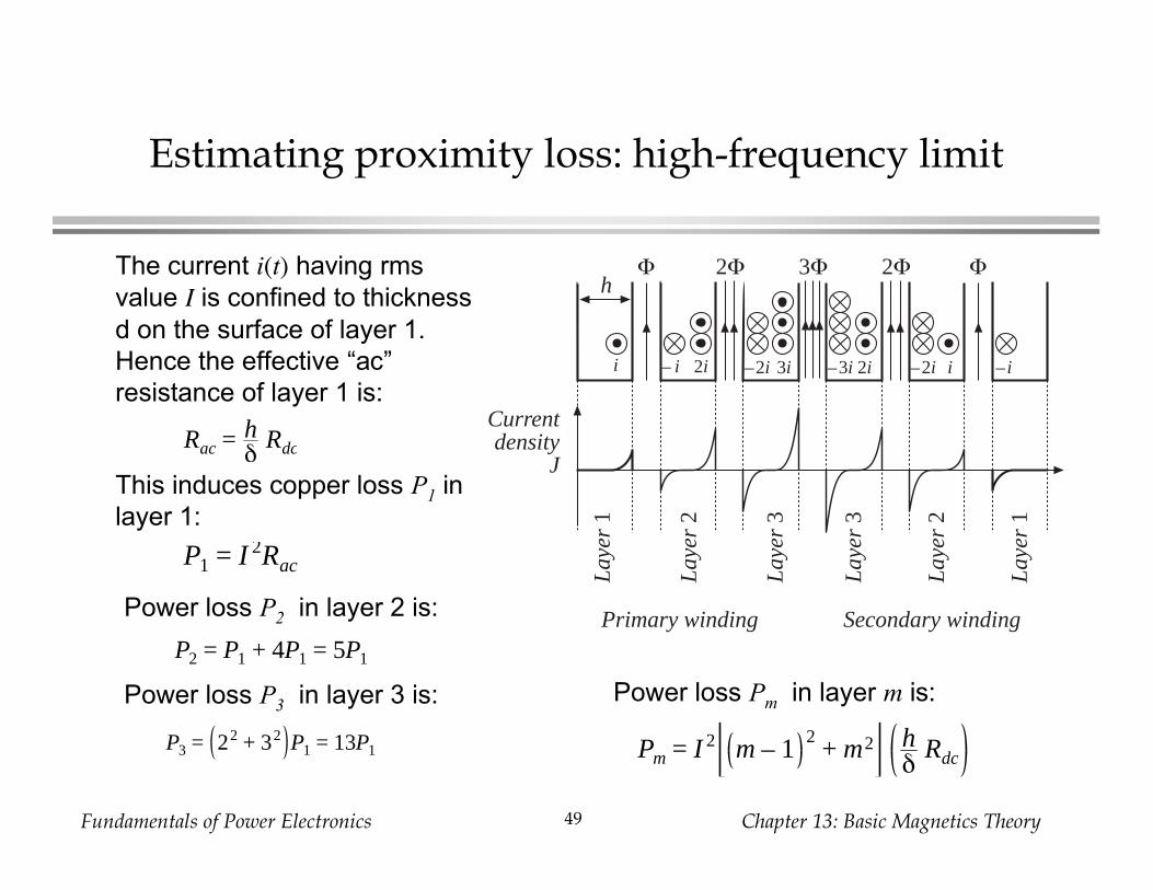
Estimating proximity loss: high-frequency limit
This induces copper loss P1 in
layer 1:
Power loss P2 in layer 2 is:
Power loss P3 in layer 3 is: Power loss Pm in layer m is:
i – i 3i–2i2i 2i –2i i –i–3i
Currentdensity
J
hΦ 2Φ 3Φ 2Φ Φ
Lay
er 1
Lay
er 2
Lay
er 3
Secondary windingPrimary winding
Lay
er 1
Lay
er 2
Lay
er 3
The current i(t) having rms
value I is confined to thickness
d on the surface of layer 1.
Hence the effective “ac”
resistance of layer 1 is:
Rac = hδ Rdc
P1 = I 2Rac
P2 = P1 + 4P1 = 5P1
P3 = 22 + 32 P1 = 13P1 Pm = I 2 m – 12
+ m2 hδ Rdc
Fundamentals of Power Electronics Chapter 13: Basic Magnetics Theory50
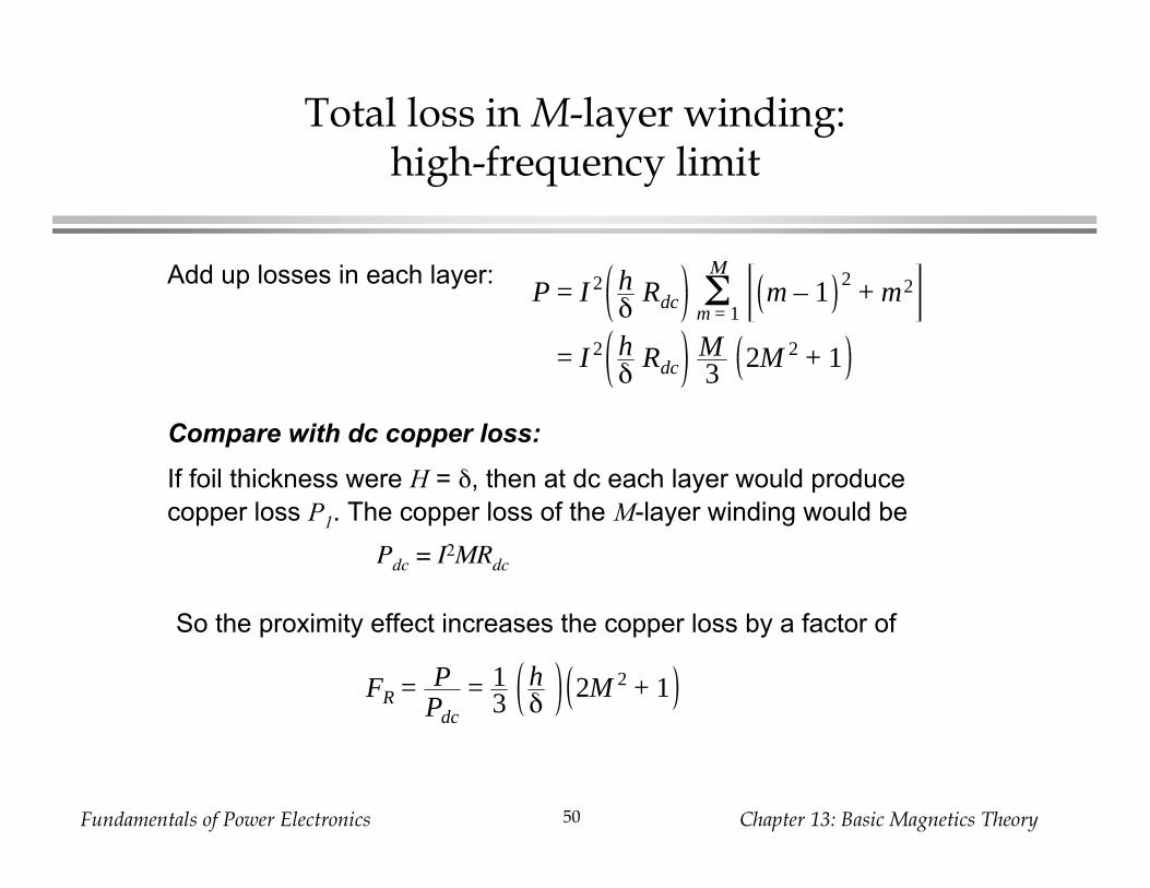
Total loss in M-layer winding:high-frequency limit
Add up losses in each layer:
Compare with dc copper loss:
If foil thickness were H = , then at dc each layer would produce
copper loss P1. The copper loss of the M-layer winding would be
So the proximity effect increases the copper loss by a factor of
P = I 2 hδ Rdc m – 1
2+ m2Σ
m = 1
Μ
= I 2 hδ Rdc
M3
2M 2 + 1
Pdc = I2MRdc
FR = PPdc
= 13
hδ 2M 2 + 1

Fundamentals of Power Electronics Chapter 13: Basic Magnetics Theory51
13.4.2 Leakage flux in windings
x
y
Primarywinding
Secondarywinding{
Coreµ > µ0
{A simple two-winding
transformer example: core and
winding geometry
Each turn carries net current i(t)
in direction shown

Fundamentals of Power Electronics Chapter 13: Basic Magnetics Theory52
Flux distribution
Leakage flux
MutualfluxΦM
Mutual flux M is large and is
mostly confined to the core
Leakage flux is present, which
does not completely link both
windings
Because of symmetry of winding
geometry, leakage flux runs
approximately vertically through
the windings
Fundamentals of Power Electronics Chapter 13: Basic Magnetics Theory53
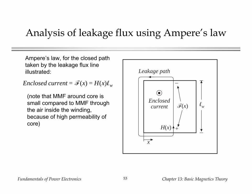
Analysis of leakage flux using Ampere’s law
x
lwF(x)
+
–
H(x)
Enclosedcurrent
Leakage path
Enclosed current = F(x) = H(x)lw
Ampere’s law, for the closed path
taken by the leakage flux line
illustrated:
(note that MMF around core is
small compared to MMF through
the air inside the winding,
because of high permeability of
core)

Fundamentals of Power Electronics Chapter 13: Basic Magnetics Theory54
Ampere’s law for the transformer example
Leakage flux
MutualfluxΦM
For the innermost leakage path,
enclosing the first layer of the
primary:
This path encloses four turns, sothe total enclosed current is 4i(t).
For the next leakage path,
enclosing both layers of the
primary:
This path encloses eight turns, sothe total enclosed current is 8i(t).
The next leakage path encloses
the primary plus four turns of the
secondary. The total enclosedcurrent is 8i(t) – 4i(t) = 4i(t).

Fundamentals of Power Electronics Chapter 13: Basic Magnetics Theory55
MMF diagram, transformer example
x
lwF(x)
+
–
H(x)
Enclosedcurrent
Leakage path
x
F(x)
Primarywinding
Secondarywinding{ {
0
8i
4i
Layer 1
Layer 2
Layer 2
Layer 1
MMF F(x) across the core window,
as a function of position x
Enclosed current = F(x) = H(x)lw

Fundamentals of Power Electronics Chapter 13: Basic Magnetics Theory56
Two-winding transformer example
Core
Lay
er 1
Lay
er 2
Lay
er 3
Lay
er 1
Lay
er 2
Lay
er 3
– i – i – ii i i
x
F(x)
i i i – i – i – i
0
i
2i
3i
MMF
Winding layout
MMF diagram
mp – ms i = F(x)
Use Ampere’s law around a
closed path taken by a leakage
flux line:
mp = number of primary
layers enclosed by path
ms = number of secondary
layers enclosed by path

Fundamentals of Power Electronics Chapter 13: Basic Magnetics Theory57
Two-winding transformer examplewith proximity effect
x
F(x)
0
i
2i
3i
MMF i – i 3i–2i2i 2i –2i i –i–3i
Flux does not
penetrate conductors
Surface currents
cause net current
enclosed by leakage
path to be zero when
path runs down
interior of a conductor
Magnetic field
strength H(x) within
the winding is given
by
H(x) =F(x)lw

Fundamentals of Power Electronics Chapter 13: Basic Magnetics Theory58
Interleaving the windings: MMF diagram
x
F(x)
i ii –i–i –i
0
i
2i
3i
MMF
pri sec pri sec pri sec
Greatly reduces the peak MMF, leakage flux, and proximity losses

Fundamentals of Power Electronics Chapter 13: Basic Magnetics Theory59
A partially-interleaved transformer
x
F(x)MMF
–3i4
–3i4
i i i –3i4
–3i4
PrimarySecondary Secondary
0
0.5 i
i
1.5 i
–0.5 i
– i
–1.5 i
m =
1
m =
1
m =
2
m =
2
m =
1.5
m =
1.5
m =
0.5
For this example,
there are three
primary layers
and four
secondary layers.
The MMF diagram
contains fractional
values.

Fundamentals of Power Electronics Chapter 13: Basic Magnetics Theory60
13.4.3 Foil windings and layers
Eliminate space between
square conductors: push
together into a single foil
turn (c)
(d) Stretch foil so its
width is lw. The adjust
conductivity so its dc
resistance is unchanged
(a) (b) (c) (d )
d
lw
h h
h
Approximating a layer of round conductors as an
effective single foil conductor:
Square conductors (b)
have same cross-
sectional area as round
conductors (a) if
h = π4
d
Fundamentals of Power Electronics Chapter 13: Basic Magnetics Theory61
Winding porosity
(c) (d )
lw
h
h
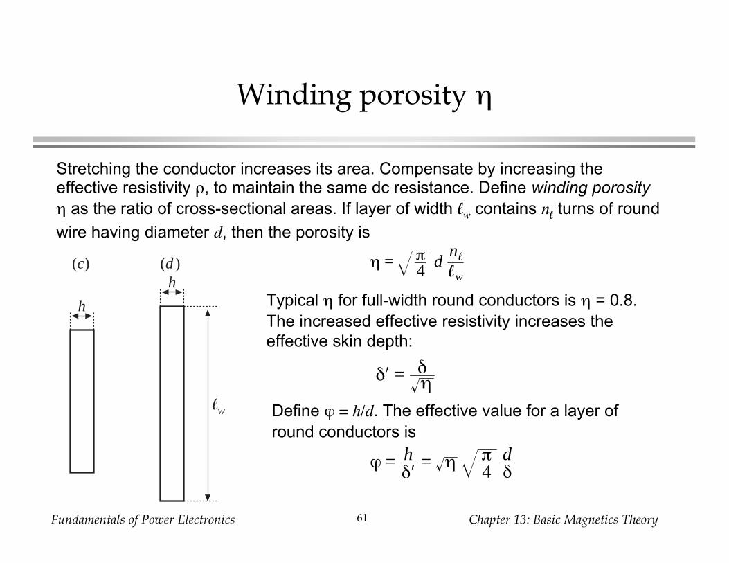
Stretching the conductor increases its area. Compensate by increasing theeffective resistivity , to maintain the same dc resistance. Define winding porosity
as the ratio of cross-sectional areas. If layer of width lw contains nl turns of round
wire having diameter d, then the porosity is
η = π4
dnl
lw
Typical for full-width round conductors is = 0.8.
The increased effective resistivity increases the
effective skin depth:
δ′ = δη
Define = h/d. The effective value for a layer of
round conductors is
ϕ = hδ′
= η π4
dδ

Fundamentals of Power Electronics Chapter 13: Basic Magnetics Theory62
13.4.4 Power loss in a layer
Approximate computation of copper loss
in one layer
Assume uniform magnetic fields at
surfaces of layer, of strengths H(0) and
H(h). Assume that these fields are
parallel to layer surface (i.e., neglect
fringing and assume field normal
component is zero).
The magnetic fields H(0) and H(h) are
driven by the MMFs F(0) and F(h).
Sinusoidal waveforms are assumed, and
rms values are used. It is assumed that
H(0) and H(h) are in phase.
F(x)
0 h
F(h)
F(0)
H(0) H(h)
Lay
er

Fundamentals of Power Electronics Chapter 13: Basic Magnetics Theory63
Solution for layer copper loss P
Solve Maxwell’s equations to find current density distribution within
layer. Then integrate to find total copper loss P in layer. Result is
wherenl = number of turns in layer,
Rdc = dc resistance of layer,
(MLT) = mean-length-per-turn,
or circumference, of layer.
P = Rdcϕnl
2 F
2(h) + F
2(0) G1(ϕ) – 4 F(h)F(0)G2(ϕ)
Rdc = ρlb
Aw= ρ
(MLT)nl3
ηlw2
G1(ϕ) =sinh (2ϕ) + sin (2ϕ)cosh (2ϕ) – cos (2ϕ)
G2(ϕ) =sinh (ϕ) cos (ϕ) + cosh (ϕ) sin (ϕ)
cosh (2ϕ) – cos (2ϕ)
η = π4
dnl
lwϕ = h
δ′= η π
4dδ

Fundamentals of Power Electronics Chapter 13: Basic Magnetics Theory64
Winding carrying current I, with nl turns per layer
If winding carries current of rms magnitude I, then
Express F(h) in terms of the winding current I, as
The quantity m is the ratio of the MMF F(h) to
the layer ampere-turns nlI. Then,
Power dissipated in the layer can now be writtenF(x)
0 h
F(h)
F(0)
H(0) H(h)
Lay
er
F(h) – F(0) = nl
I
F(h) = mnl
I
F(0)F(h)
= m – 1m
P = I 2RdcϕQ′(ϕ, m)
Q′(ϕ, m) = 2m2 – 2m + 1 G1(ϕ) – 4m m – 1 G2(ϕ)

Fundamentals of Power Electronics Chapter 13: Basic Magnetics Theory65
Increased copper loss in layer
P = I 2RdcϕQ′(ϕ, m)
1
10
100
0.1 1 10
ϕ
PI 2Rdc
m = 0.5
1
1.5
2
345681012m = 15

Fundamentals of Power Electronics Chapter 13: Basic Magnetics Theory66
Layer copper loss vs. layer thickness
Relative to copperloss when h =
PPdc ϕ = 1
= Q′(ϕ, m)
0.1 1 100.1
1
10
100
ϕ
m = 0.5
1
1.5
2
3
4
5
6
81012m = 15
PPdc ϕ = 1

Fundamentals of Power Electronics Chapter 13: Basic Magnetics Theory67
13.4.5 Example: Power loss ina transformer winding
Two winding
transformer
Each windingconsists of M layers
Proximity effect
increases copper
loss in layer m by
the factor
Sum losses over all
primary layers:
{x
npi npi npi npi npi npi
Primary layers Secondary layers{F
0npi
2npi
Mnpi
m =
1
m =
2
m =
M
m =
M
m =
2
m =
1
FR =Ppri
Ppri,dc= 1
M ϕQ′(ϕ, m)Σm = 1
M
Q ( ,m)

Fundamentals of Power Electronics Chapter 13: Basic Magnetics Theory68
Increased total winding lossExpress summation in
closed form:
1
10
100
1010.1
0.5
1
1.5
2
3
ϕ
45678101215Number of layers M =
FR =Ppri
Ppri,dc
FR = ϕ G1(ϕ) + 23
M 2 – 1 G1(ϕ) – 2G2(ϕ)
Fundamentals of Power Electronics Chapter 13: Basic Magnetics Theory69
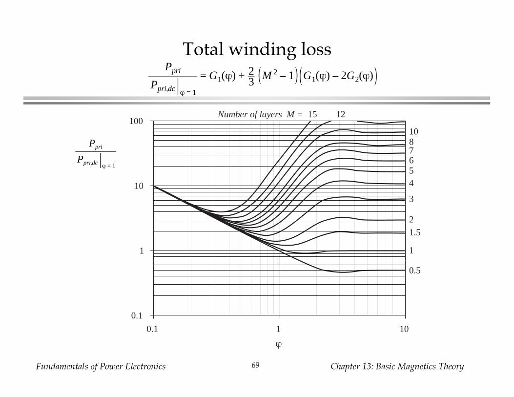
Total winding loss
0.1
1
10
100
0.1 1 10
0.5
1
1.52
3
4567810
1215Number of layers M =
ϕ
Ppri
Ppri,dc ϕ = 1
Ppri
Ppri,dc ϕ = 1
= G1(ϕ) + 23
M 2 – 1 G1(ϕ) – 2G2(ϕ)
Fundamentals of Power Electronics Chapter 13: Basic Magnetics Theory70
13.4.6 Interleaving the windings
x
F(x)
i ii –i–i –i
0
i
2i
3i
MMF
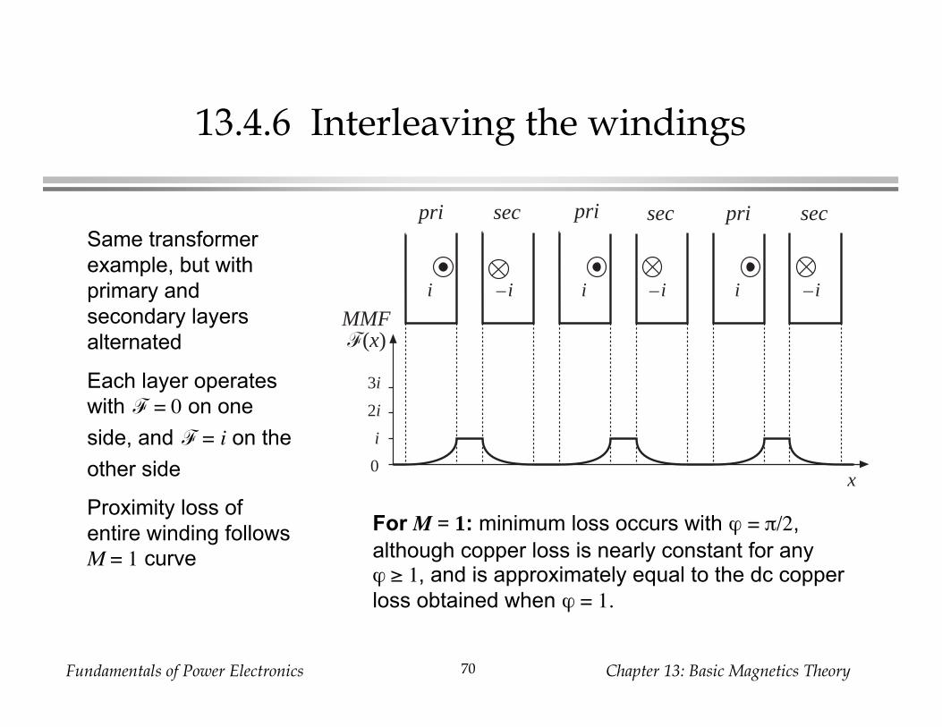
pri sec pri sec pri secSame transformer
example, but with
primary and
secondary layers
alternated
Each layer operates
with F = 0 on one
side, and F = i on the
other side
Proximity loss of
entire winding follows
M = 1 curve
For M = 1: minimum loss occurs with = /2,
although copper loss is nearly constant for any1, and is approximately equal to the dc copper
loss obtained when = 1.

Fundamentals of Power Electronics Chapter 13: Basic Magnetics Theory71
Partial interleaving
x
F(x)MMF
–3i4
–3i4
i i i –3i4
–3i4
PrimarySecondary Secondary
0
0.5 i
i
1.5 i
–0.5 i
– i
–1.5 i
m =
1
m =
1
m =
2
m =
2
m =
1.5
m =
1.5
m =
0.5
Partially-interleaved
example with 3 primary and
4 secondary layers
Each primary layer carriescurrent i while each
secondary layer carries0.75i. Total winding currents
add to zero. Peak MMF
occurs in space between
windings, but has value 1.5i.
We can apply the previous solution for the copper loss in each layer, and add the
results to find the total winding losses. To determine the value of m to use for a
given layer, evaluate
m =F(h)
F(h) – F(0)

Fundamentals of Power Electronics Chapter 13: Basic Magnetics Theory72
Determination of m
x
F(x)MMF
–3i4
–3i4
i i i –3i4
–3i4
PrimarySecondary Secondary
0
0.5 i
i
1.5 i
–0.5 i
– i
–1.5 i
m =
1
m =
1
m =
2
m =
2
m =
1.5
m =
1.5
m =
0.5
m =F(h)
F(h) – F(0)= – 0.75i
– 0.75i – 0= 1
Leftmost secondary layer:
m =F(h)
F(h) – F(0)= – 1.5i
– 1.5i – (– 0.75i)= 2
Next secondary layer:
Next layer (primary):
m =F(0)
F(0) – F(h)= – 1.5i
– 1.5i – (– 0.5i)= 1.5
Center layer (primary):
m =F(h)
F(h) – F(0)= 0.5i
0.5i – (– 0.5i)= 0.5 Use the plot for layer loss (repeated on
next slide) to find loss for each layer,
according to its value of m. Add results to
find total loss.

Fundamentals of Power Electronics Chapter 13: Basic Magnetics Theory73
Layer copper loss vs. layer thickness
Relative to copperloss when h =
PPdc ϕ = 1
= Q′(ϕ, m)
0.1 1 100.1
1
10
100
ϕ
m = 0.5
1
1.5
2
3
4
5
6
81012m = 15
PPdc ϕ = 1

Fundamentals of Power Electronics Chapter 13: Basic Magnetics Theory74
Discussion: design of winding geometryto minimize proximity loss
• Interleaving windings can significantly reduce the proximity loss when
the winding currents are in phase, such as in the transformers of buck-
derived converters or other converters
• In some converters (such as flyback or SEPIC) the winding currents are
out of phase. Interleaving then does little to reduce the peak MMF and
proximity loss. See Vandelac and Ziogas [10].
• For sinusoidal winding currents, there is an optimal conductor thicknessnear = 1 that minimizes copper loss.
• Minimize the number of layers. Use a core geometry that maximizes
the width lw of windings.
• Minimize the amount of copper in vicinity of high MMF portions of the
windings

Fundamentals of Power Electronics Chapter 13: Basic Magnetics Theory75
Litz wire
• A way to increase conductor area while maintaining lowproximity losses
• Many strands of small-gauge wire are bundled together and areexternally connected in parallel
• Strands are twisted, or transposed, so that each strand passesequally through each position on inside and outside of bundle.This prevents circulation of currents between strands.
• Strand diameter should be sufficiently smaller than skin depth
• The Litz wire bundle itself is composed of multiple layers
• Advantage: when properly sized, can significantly reduceproximity loss
• Disadvantage: increased cost and decreased amount of copperwithin core window

Fundamentals of Power Electronics Chapter 13: Basic Magnetics Theory76
13.4.7 PWM waveform harmonics
Fourier series:
with
Copper loss:
Dc
Ac
Total, relative to value predicted by low-frequency analysis:
t
i(t)Ipk
DTs Ts0
i(t) = I0 + 2 I j cos ( jωt)Σj = 1
∞
I j =2 I pk
jπ sin ( jπD) I0 = DIpk
Pdc = I 02Rdc
Pj = I j2Rdc j ϕ1 G1( j ϕ1) + 2
3M 2 – 1 G1( j ϕ1) – 2G2( j ϕ1)
Pcu
DI pk2 Rdc
= D +2ϕ1
Dπ2sin2 ( jπD)
j jG1( j ϕ1) + 2
3M 2 – 1 G1( j ϕ1) – 2G2( j ϕ1)Σ
j = 1
∞

Fundamentals of Power Electronics Chapter 13: Basic Magnetics Theory77
Harmonic loss factor FH
Effect of harmonics: FH = ratio of total ac copper loss to fundamental
copper loss
The total winding copper loss can then be written
FH =PjΣ
j = 1
∞
P1
Pcu = I 02Rdc + FH FR I 1
2Rdc

Fundamentals of Power Electronics Chapter 13: Basic Magnetics Theory78
Increased proximity lossesinduced by PWM waveform harmonics: D = 0.5
1
10
0.1 1 10ϕ1
FH
D = 0.5
M = 0.5
1
1.5
2
3
4
5
6
8
M = 10

Fundamentals of Power Electronics Chapter 13: Basic Magnetics Theory79
Increased proximity losses induced by PWMwaveform harmonics: D = 0.3
1
10
100
0.1 1 10ϕ1
FH
M = 0.5
11.5
2
34
5
68
M = 10
D = 0.3

Fundamentals of Power Electronics Chapter 13: Basic Magnetics Theory80
Increased proximity losses induced by PWMwaveform harmonics: D = 0.1
1
10
100
0.1 1 10ϕ1
FH
M = 0.5
1
1.5
2
34
56
8M = 10 D = 0.1

Fundamentals of Power Electronics Chapter 13: Basic Magnetics Theory81
Discussion: waveform harmonics
• Harmonic factor FH accounts for effects of harmonics
• Harmonics are most significant for 1 in the vicinity of 1
• Harmonics can radically alter the conclusion regarding optimalwire gauge
• A substantial dc component can drive the design towards largerwire gauge
• Harmonics can increase proximity losses by orders ofmagnitude, when there are many layers and when 1 lies in thevicinity of 1
• For sufficiently small 1, FH tends to the value 1 + (THD)2, wherethe total harmonic distortion of the current is
THD =I j
2Σj = 2
∞
I1

Fundamentals of Power Electronics Chapter 13: Basic Magnetics Theory82
13.5. Several types of magnetic devices, theirB–H loops, and core vs. copper loss
A key design decision: the choice of maximum operating flux density Bmax
• Choose Bmax to avoid saturation of core, or
• Further reduce Bmax , to reduce core losses
Different design procedures are employed in the two cases.
Types of magnetic devices:
Filter inductor AC inductor
Conventional transformer Coupled inductor
Flyback transformer SEPIC transformer
Magnetic amplifier Saturable reactor

Fundamentals of Power Electronics Chapter 13: Basic Magnetics Theory83
Filter inductor
CCM buck example
+–
L
i(t)
i(t)
t0 DTsTs
I ∆iL
B
Hc0
∆Hc
Hc
Bsat
Minor B–H loop,filter inductor
B–H loop,large excitation
∆B
H c(t) =ni(t)lc
Rc
Rc + Rg

Fundamentals of Power Electronics Chapter 13: Basic Magnetics Theory84
Filter inductor, cont.
• Negligible core loss, negligible
proximity loss
• Loss dominated by dc copper
loss
• Flux density chosen simply to
avoid saturation
• Air gap is employed
• Could use core materials
having high saturation flux
density (and relatively high
core loss), even though
converter switching frequency
is high
Air gapreluctanceRg
nturns
i(t)
Φ
Core reluctance Rc
+v(t)–
+–ni(t) Φ(t)
Rc
Rg
Fc+ –

Fundamentals of Power Electronics Chapter 13: Basic Magnetics Theory85
AC inductor
L
i(t)
i(t)
t
∆i
∆i
B
∆Hc Hc
Bsat
B–H loop, foroperation asac inductor
Core B–H loop
–∆Hc
∆B
–∆B

Fundamentals of Power Electronics Chapter 13: Basic Magnetics Theory86
AC inductor, cont.
• Core loss, copper loss, proximity loss are all significant
• An air gap is employed
• Flux density is chosen to reduce core loss
• A high-frequency material (ferrite) must be employed

Fundamentals of Power Electronics Chapter 13: Basic Magnetics Theory87
Conventional transformer
n1 : n2
+
v1(t)
–
+
v2(t)
–
i1(t) i2(t)
LM
iM(t)
iM(t)
t
∆iM
v1(t) Area λ1
B–H loop, foroperation asconventionaltransformer
B
Hc
Core B–H loop
λ1
2n1Ac
n1∆imp
lm
H(t) =niM(t)lm

Fundamentals of Power Electronics Chapter 13: Basic Magnetics Theory88
Conventional transformer, cont.
• Core loss, copper loss, and proximity loss are usually significant
• No air gap is employed
• Flux density is chosen to reduce core loss
• A high frequency material (ferrite) must be employed
Fundamentals of Power Electronics Chapter 13: Basic Magnetics Theory89
Coupled inductor
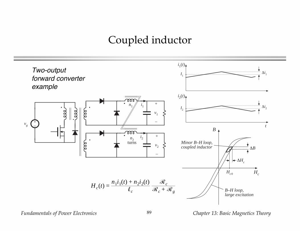
Two-outputforward converterexample
n1+
v1
–
n2turns
i1
+
v2
–
i2
+–vg
i1(t)
I1∆i1
i2(t)
t
I2∆i2
B
Hc0
∆Hc
Hc
Minor B–H loop,coupled inductor
B–H loop,large excitation
∆B
H c(t) =n1i1(t) + n2i2(t)
lc
Rc
Rc + Rg

Fundamentals of Power Electronics Chapter 13: Basic Magnetics Theory90
Coupled inductor, cont.
• A filter inductor having multiple windings
• Air gap is employed
• Core loss and proximity loss usually not significant
• Flux density chosen to avoid saturation
• Low-frequency core material can be employed

Fundamentals of Power Electronics Chapter 13: Basic Magnetics Theory91
DCM flyback transformer
+–
LM
+
v
–vg
n1 : n2
iMi1 i2
i1(t) i1,pk
i2(t)
tiM(t)
t
i1,pk
B–H loop, foroperation inDCM flybackconverter
B
Hc
Core B–H loop
n1i1,pk
lm
Rc
Rc+Rg
∆B
∆B

Fundamentals of Power Electronics Chapter 13: Basic Magnetics Theory92
DCM flyback transformer, cont.
• Core loss, copper loss, proximity loss are significant
• Flux density is chosen to reduce core loss
• Air gap is employed
• A high-frequency core material (ferrite) must be used

Fundamentals of Power Electronics Chapter 13: Basic Magnetics Theory93
Summary of Key Points
1. Magnetic devices can be modeled using lumped-element magnetic
circuits, in a manner similar to that commonly used to model electrical
circuits. The magnetic analogs of electrical voltage V, current I, and
resistance R, are magnetomotive force (MMF) F, flux , and reluctance R
respectively.
2. Faraday’s law relates the voltage induced in a loop of wire to the derivative
of flux passing through the interior of the loop.
3. Ampere’s law relates the total MMF around a loop to the total current
passing through the center of the loop. Ampere’s law implies that winding
currents are sources of MMF, and that when these sources are included,
then the net MMF around a closed path is equal to zero.
4. Magnetic core materials exhibit hysteresis and saturation. A core material
saturates when the flux density B reaches the saturation flux density Bsat.

Fundamentals of Power Electronics Chapter 13: Basic Magnetics Theory94
Summary of key points
5. Air gaps are employed in inductors to prevent saturation when a given
maximum current flows in the winding, and to stabilize the value of
inductance. The inductor with air gap can be analyzed using a simple
magnetic equivalent circuit, containing core and air gap reluctances and a
source representing the winding MMF.
6. Conventional transformers can be modeled using sources representing the
MMFs of each winding, and the core MMF. The core reluctance
approaches zero in an ideal transformer. Nonzero core reluctance leads to
an electrical transformer model containing a magnetizing inductance,
effectively in parallel with the ideal transformer. Flux that does not link both
windings, or “leakage flux,” can be modeled using series inductors.
7. The conventional transformer saturates when the applied winding volt-
seconds are too large. Addition of an air gap has no effect on saturation.
Saturation can be prevented by increasing the core cross-sectional area,
or by increasing the number of primary turns.

Fundamentals of Power Electronics Chapter 13: Basic Magnetics Theory95
Summary of key points
8. Magnetic materials exhibit core loss, due to hysteresis of the B–H loop and
to induced eddy currents flowing in the core material. In available core
materials, there is a tradeoff between high saturation flux density Bsat and
high core loss Pfe. Laminated iron alloy cores exhibit the highest Bsat but
also the highest Pfe, while ferrite cores exhibit the lowest Pfe but also the
lowest Bsat. Between these two extremes are powdered iron alloy and
amorphous alloy materials.
9. The skin and proximity effects lead to eddy currents in winding conductors,
which increase the copper loss Pcu in high-current high-frequency magnetic
devices. When a conductor has thickness approaching or larger than thepenetration depth , magnetic fields in the vicinity of the conductor induce
eddy currents in the conductor. According to Lenz’s law, these eddy
currents flow in paths that tend to oppose the applied magnetic fields.

Fundamentals of Power Electronics Chapter 13: Basic Magnetics Theory96
Summary of key points
10. The magnetic field strengths in the vicinity of the winding conductors can
be determined by use of MMF diagrams. These diagrams are constructed
by application of Ampere’s law, following the closed paths of the magnetic
field lines which pass near the winding conductors. Multiple-layer
noninterleaved windings can exhibit high maximum MMFs, with resulting
high eddy currents and high copper loss.
11. An expression for the copper loss in a layer, as a function of the magnetic
field strengths or MMFs surrounding the layer, is given in Section 13.4.4.
This expression can be used in conjunction with the MMF diagram, to
compute the copper loss in each layer of a winding. The results can then
be summed, yielding the total winding copper loss. When the effective
layer thickness is near to or greater than one skin depth, the copper losses
of multiple-layer noninterleaved windings are greatly increased.

Fundamentals of Power Electronics Chapter 13: Basic Magnetics Theory97
Summary of key points
12. Pulse-width-modulated winding currents of contain significant total
harmonic distortion, which can lead to a further increase of copper loss.
The increase in proximity loss caused by current harmonics is most
pronounced in multiple-layer non-interleaved windings, with an effective
layer thickness near one skin depth.
13. A variety of magnetic devices are commonly used in switching converters.These devices differ in their core flux density variations, as well as in themagnitudes of the ac winding currents. When the flux density variationsare small, core loss can be neglected. Alternatively, a low-frequencymaterial can be used, having higher saturation flux density.
Recommended