Identification of Larval Moxostoma (Catostomidae) from the Oconee
River, Georgia
by
J. Stuart Carlton
(Under the direction of Cecil A. Jennings)
Abstract
Robust redhorse, Moxostoma robustum, is a recently rediscovered, imperiled
species of sucker (Catostomidae) that inhabits several rivers in the Atlantic Slope
drainage and is subject to intense conservation efforts. Its spawning period
frequently overlaps that of a sympatric congener, the notchlip redhorse (M.
collapsum), making identifying the larvae of the species difficult. I measured various
morphometrics, meristics, and developmental characteristics on lab-reared larvae of
each species, fit a classification tree model to the data, and used the model to create
a key discriminating between the species. The model had a leave-one-out,
cross-validation expected error rate of 4.7%. The key formed from the model is
highly accurate for fishes from 10–20 mm total length: three independent verifiers
used the key to identify fishes with a 95% accuracy rate. This key is one of a few
that distinguishes between sympatric Moxostoma larvae and is the first to identify
larval robust redhorse.
Index words: Robust redhorse, Moxostoma robustum, Notchlip redhorse,Moxostoma collapsum, Taxonomic key, Oconee River,Catostomidae, Larval fishes, CATDAT, Classification trees,Robust Redhorse Conservation Committee

Identification of Larval Moxostoma (Catostomidae) from the Oconee
River, Georgia
by
J. Stuart Carlton
B.A., Tulane University, 2001
A Thesis Submitted to the Graduate Faculty
of The University of Georgia in Partial Fulfillment
of the
Requirements for the Degree
Master of Science
Athens, Georgia
2004

c© 2004
J. Stuart Carlton
All Rights Reserved

Identification of Larval Moxostoma (Catostomidae) from the Oconee
River, Georgia
by
J. Stuart Carlton
Approved:
Major Professor: Cecil A. Jennings
Committee: Byron J. Freeman
James T. Peterson
Electronic Version Approved:
Maureen Grasso
Dean of the Graduate School
The University of Georgia
December 2004

Acknowledgments
Funding for this project was provided by the Athens office of the US Fish and
Wildlife Service and Georgia Power. Thanks is due to the Georgia Coop Unit and
the Warnell School of Forest Resources at the University of Georgia for providing
facilities and, of course, my education. I’d also like to thank Dr. Hank Bart; without
his advice and encouragement I’d probably still be selling beer at sporting events.
I received good technical advice from Nancy Auer, Rebecca Cull, David
Higginbotham, Haile MacCurdy, Wayne Starnes, Darrel Snyder, Paul Vecsei, and
Richard Weyers. My crew of technicians, who did much of the difficult work for this
project, included Gene Crouch, Peter Dimmick, Tavis McLean, Diarra Mosely, Dave
Shepard, and Steve Zimpfer. Bob Wallus made many of the measurements used in
my research and provided the written narratives in Appendices C and D.
My advisory committee was particularly helpful because of my non-scientific
background. Dr. Bud Freeman gave me wonderful advice on how to be a scientist.
Dr. Jim Peterson helped me understand the philosophy lurking behind the statistics,
and provided valuable computer programming assistance. Dr. Cecil Jennings was my
committee chair, field hand, confidant, and mentor. He taught me the importance of
maintaining balance in life and was wise enough to let me make my own mistakes.
He also showed me how to straighten out a trailered boat using a tree trunk.
I’d like to thank my family for putting up with me. I owe my sense of humor to
my mom; without it I wouldn’t have finished this project. My dad is my fishing
buddy, and is kind enough to re-rig my pole while I fish with his. Thanks, Dad.
Finally, I’d like to thank Libby for inspiring me to be my best, comforting me when
I wasn’t, and teaching me the value of a good checklist.
iv
Table of Contents
Page
Acknowledgments . . . . . . . . . . . . . . . . . . . . . . . . . . . . . . iv
List of Figures . . . . . . . . . . . . . . . . . . . . . . . . . . . . . . . . vi
List of Tables . . . . . . . . . . . . . . . . . . . . . . . . . . . . . . . . vii
Chapter
1 Introduction . . . . . . . . . . . . . . . . . . . . . . . . . . . . . 1
2 Literature Review . . . . . . . . . . . . . . . . . . . . . . . . . . 7
3 Methods . . . . . . . . . . . . . . . . . . . . . . . . . . . . . . . . 14
4 Results . . . . . . . . . . . . . . . . . . . . . . . . . . . . . . . . . 20
5 Discussion . . . . . . . . . . . . . . . . . . . . . . . . . . . . . . . 29
Bibliography . . . . . . . . . . . . . . . . . . . . . . . . . . . . . . . . . 35
Appendix
A Key for Identifying Larval Moxostoma in the Oconee River,
Georgia . . . . . . . . . . . . . . . . . . . . . . . . . . . . . . . . 43
B Characters Measured for the Classification Tree . . . . . . 46
C Development of Young Robust Redhorse . . . . . . . . . . . 56
D Development of Young Notchlip Redhorse . . . . . . . . . . 63
E Morphometric and Descriptive Measurements . . . . . . . . 72
v

List of Figures
1.1 Length-frequency distribution for larval Moxostoma collected May–
November 1996 . . . . . . . . . . . . . . . . . . . . . . . . . . . . . . 4
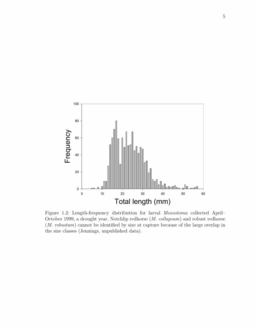
1.2 Length-frequency distribution for larval Moxostoma collected April–
October 1999 . . . . . . . . . . . . . . . . . . . . . . . . . . . . . . . 5
3.1 Morphometrics measured on notchlip and robust redhorse . . . . . . . 17
4.1 Standard length in laboratory-reared larval notchlip and robust redhorse 21
4.2 Pre-anal length in laboratory-reared larval notchlip and robust redhorse 21
4.3 Pre-dorsal fin length in laboratory-reared larval notchlip and robust
redhorse . . . . . . . . . . . . . . . . . . . . . . . . . . . . . . . . . . 22
4.4 Greatest body depth in laboratory-reared larval notchlip and robust
redhorse . . . . . . . . . . . . . . . . . . . . . . . . . . . . . . . . . . 22
4.5 Head length in laboratory-reared larval notchlip and robust redhorse . 23
4.6 Eye diameter in laboratory-reared larval notchlip and robust redhorse 23
4.7 Classification tree for the identification of larval notchlip and robust
redhorse . . . . . . . . . . . . . . . . . . . . . . . . . . . . . . . . . . 26
4.8 Continuation of the classification tree for the identification of larval
notchlip and robust redhorse . . . . . . . . . . . . . . . . . . . . . . . 26
vi

List of Tables
4.1 Descriptive and ontogenetic traits used in the classification tree model 24
4.2 Description of traits used in the classification tree model . . . . . . . 27
B.1 Descriptive and ontogenetic traits measured on notchlip and robust
redhorse . . . . . . . . . . . . . . . . . . . . . . . . . . . . . . . . . . 46
B.2 Description of traits measured on larval robust notchlip and robust
redhorse . . . . . . . . . . . . . . . . . . . . . . . . . . . . . . . . . . 50
E.1 Morphometric and descriptive character measurements made on larval
notchlip and robust redhorse and fit to a classification tree model . . 73
vii

Chapter 1
Introduction
Robust redhorse (Moxostoma robustum) is a poorly known imperiled species of
large, riverine sucker (Teleostei: Catostomidae). Originally described as
Ptychostomus robustus by Edward Drinker Cope in 1870 (Cope 1870), robust
redhorse are presumed to be endemic to Piedmont and upper Coastal Plain rivers
along the Atlantic Slope drainage from the Pee Dee River in North Carolina to the
Altamaha River system in middle Georgia (Evans 1994). Anthropomorphic changes
to these rivers in the late 19th and early 20th centuries likely limited the habitat
available to robust redhorse, thereby greatly reducing their overall abundance
(Evans 1994). Overfishing also probably contributed to the population decline: they
were a widely-sought and heavily-harvested food fish in the 19th century (Cope
1870). Cope’s specimens were lost while being relocated (Bryant et al. 1996), and
the scientific community’s knowledge of robust redhorse disappeared with them
(Evans 1994). Indeed, the specific name robustus was errantly given to another fish
(Jenkins and Burkhead 1993).
In 1980, a robust redhorse was caught in the Savannah River, Georgia and
misidentified as a regional variant of the river redhorse (M. carinatum) (Jenkins and
Burkhead 1993). In 1985, another robust redhorse was caught in the Pee Dee River
in South Carolina and was similarly misidentified (Jenkins and Burkhead 1993). In
1991, five more robust redhorse were collected from the Oconee River in Georgia
(Evans 1994). Taxonomists, including Dr. Hank Bart, Dr. Byron Freeman, and Dr.
Robert Jenkins (Bryant et al. 1996), were perplexed by these catches and, after
1

2
reviewing regional catostomid systematics, they determined that the fish they had
identified as previously as a variant of M. carinatum were actually robust redhorse,
resurfacing after a 100 year absence (Jenkins and Burkhead 1993). The species was
rechristened M. robustum to conform with modern phylogenetic theory (Jenkins and
Burkhead 1993), and scientists began working to determine the species’ modern
range and what steps could be taken to conserve the rare fish (Evans 1996).
In 1995, a diverse group of stakeholders, including state and federal resource
agencies, universities, and private industrial companies, formed the Robust Redhorse
Conservation Committee (RRCC) to oversee the conservation efforts of the newly
rediscovered fish (Evans 1996). The goal of the RRCC is to reestablish robust
redhorse in sustainable numbers throughout its historical range without resorting to
listing the species under the Federal Endangered Species Act (Evans 1996).
Members of the RRCC have undertaken diverse projects toward this goal, including
assessments of artificial propagation techniques (Barrett 1997; Higginbotham and
Jennings 1999), annual population assessments (e.g., Jennings et al. 2000), genetic
determination of population diversity (Wirgin 2002), telemetric tracking studies
(Cecil A. Jennings, Georgia Cooperative Fish and Wildlife Research Unit, personal
communication), and various stocking regimes (e.g., Freeman et al. 2002).
These projects have achieved measured success. RRCC-approved research and
field work have led to the discovery of wild populations of robust redhorse in the
Oconee and Ocmulgee rivers in Georgia, the Savannah River in Georgia and South
Carolina, and the Pee Dee River in North Carolina (DeMeo 2001). Additionally, the
RRCC has established small stocked populations in the Ocmulgee, Broad, and
Ogeechee rivers in Georgia (DeMeo 2001). The successes of the RRCC have been
many, but there are still many critical areas where the understanding of robust
redhorse is incomplete.

3
Population recruitment is one such area. Age-0 redhorse rarely have been found
during the annual population assessments (Jennings et al. 1996). Additionally,
RRCC members have collected few robust redhorse between the sizes of 15 mm and
400 mm total length and don’t know how many robust redhorse survive past this
length or what happens to them if they do (DeMeo 2001). These facts suggest that
population recruitment may be limited (Jennings et al. 1996).
Understanding the population dynamics and ecology of the larvae may aid in
discovering the plight of the would-be recruits. To this end, the RRCC has
undertaken a variety of laboratory-based larval studies, including
swimming-strength evaluations (Ruetz III 1997), a study of the effects of gravel
quality on larval survival (Dilts 1999), and testing larval survival in various water
flow regimes (Weyers 2000). There also have been annual field studies of larval
abundance (Jennings, personal communication), but the data have been difficult to
analyze, as robust redhorse larvae are very similar in appearance to the larvae of a
sympatric congener, the notchlip redhorse (Moxostoma collapsum) (Wirgin et al.
2004). During spawning seasons with normal amounts of rain, robust and notchlip
redhorse spawn 3–6 weeks apart (see “Biology and Spawning Behavior”, below), and
their larvae are easy to distinguish based on size at capture (Figure 1.1) (Jennings,
personal communication). However, during years of abnormally low rainfall, the
spawning period of robust and notchlip redhorse is compressed, and size at capture
is not an effective means of distinguishing between them (Figure 1.2) (Jennings,
personal communication). One must use other methods.
A highly accurate alternative means of identification is to use unique genetic
identifiers within the fishes (Wirgin et al. 2004). However, this process is expensive
and time-consuming, (Jennings, personal communication). A taxonomic key
discriminating between the two species would facilitate the analysis of larval
abundance data by providing an inexpensive and quick method for identifying the

4
Figure 1.1: Length-frequency distribution for larval Moxostoma collected May–November 1996, a “normal” rain year. The larger clusters (above 35 mm total length)are assumed to be notchlip redhorse (M. collapsum) and the smallest one is assumedto be robust redhorse (M. robustum) (Jennings, unpublished data).
5
Figure 1.2: Length-frequency distribution for larval Moxostoma collected April–October 1999, a drought year. Notchlip redhorse (M. collapsum) and robust redhorse(M. robustum) cannot be identified by size at capture because of the large overlap inthe size classes (Jennings, unpublished data).

6
species, ideally while limiting the loss of accuracy compared to using genetic
identification. The goal of this project is to create such a key.
Biology and Spawning Behavior
Robust redhorse are typical members of genus Moxostoma: large, riverine,
bottom-feeding, and generally invertivorous, with an inferior mouth and thick,
fleshy lips (Jenkins and Burkhead 1993). One of the larger members of the genus,
robust redhorse can grow to 760 mm and reach 8 kg (Walsh et al. 1998). They are
among the most long-lived of the Moxostoma, often surpassing 20 years of age
(Evans 1994), compared to the 8–15 years of other redhorse (Jenkins and Burkhead
1993). Robust redhorse gather in the spring near shoals and flats to spawn over
coarse gravel substrate (Jennings et al. 1996). They spawn in groups of one female
and two or three males, quivering in unison to stir up the gravel as they release
their gametes (Jennings et al. 1996). Shuffling the gravel allows them to deposit
their eggs in the interstices at depths approaching 15 cm (Jennings et al. 1996). In
Georgia, spawning usually occurs from late April to early June, when water
temperatures reach approximately 19–20 ◦C (Jennings et al. 1996).
Notchlip redhorse are similar in appearance to robust redhorse. However, they
are slightly smaller when fully grown, with a maximum size of approximately 700
mm and 5 kg (Weyers 2000). Notchlip redhorse spawn in a similar manner to their
sister species (Jenkins and Burkhead 1993), gathering when the water temperatures
rise above 10 ◦C (Weyers 2000). In Georgia, this can occur anywhere from
mid-March to late April (Weyers 2000).

Chapter 2
Literature Review
Proper species identification is an essential part of ecological research. Identifying
fish requires a consistent protocol to ensure accuracy and precision. Identifying
fishes often is a difficult task, and poorly-explained or improperly followed protocols
can render it impossible.
Identification of Adult Fishes
The basic methodology for identifying adult fishes has been in place for over a
century. Edward Drinker Cope, who described over 300 new species of fish between
1862 and 1894 (Academy of Natural Sciences 2004), devised many of the
characteristics that are used to identify adult fishes today. However, the
characteristics weren’t standardized, and taxonomists’ work was subjective and
difficult to repeat (Hubbs and Lagler 1958). Subjectivity was the rule until 1958,
when Carl L. Hubbs and Karl F. Lagler published Fishes of the Great Lakes Region,
which contained the the first widely-available attempt to standardize the definitions
of the most commonly used taxonomic characters (Hubbs and Lagler 1958).
Taxonomic characters are divided into two main categories: meristics and
morphometrics. Meristics, which are generally the more reliable of the two (Fuiman
1979) are aspects of a fish that can be counted (Hubbs and Lagler 1958). Commonly
useful external meristics for identifying adult fishes include number of scales along
7

8
the lateral line; number of pre-dorsal scales; number of circumpeduncal scales; and
dorsal, anal, caudal, pectoral, and pelvic fin ray counts (Strauss and Bond 1990).
Commonly useful internal meristics include number of gill rakers, amount of various
types of dentition, and number of vertebrae (Strauss and Bond 1990). Meristic traits
are useful because they usually are easy to count, but they can be influenced by
environmental factors, especially temperature (Lindsey 1958; Lindsey 1962; Barlow
1961).
Morphometrics are body measurements and proportions (Hubbs and Lagler
1958). The most common include head length, snout length, eye orbit length, body
depth, pre-anal length, length of the longest dorsal fin ray, and the heights of
various fins. These measures usually are expressed as a percentage of the standard
length or total length of the specimen to remove the effects of the size of the fish
(Strauss and Bond 1990). Morphometrics can be affected by environmental factors
— particularly diet — throughout the life of the fish, which can limit their
diagnostic utility (Snyder and Muth 1990; Van Velzen et al. 1998).
In addition to meristics and morphometrics, other anatomical characters, such
as pigmentation, descriptions of lateral line shape, position, and completeness, and
secondary sexual characteristics, such as the presence or absence of breeding
tubercles, often are used on a case-by-case basis (Strauss and Bond 1990). The
appearance of unusual characters often provides conclusive evidence to a difficult
taxonomic problem. As with meristics and morphometrics, anatomical traits —
especially pigmentation (Bolker and Hill 2000) — can be affected by environmental
conditions, so they must be used judiciously (Snyder and Muth 1990).
Identification of Larval Fishes
The technique for identifying larval fishes is similar to that for identifying adult
fishes. However, many of the adult characters are not present or are less-developed

9
in larval fishes, and are ineffective for discriminating between species (Snyder and
Muth 1990). A taxonomist often must use modified versions of adult characters or
unique larval characters to discriminate among larval fishes (Methven and
McGowan 1998). The effective — and present — characters vary among families
and even among genera (Snyder and Muth 1990). Additionally, larval fish characters
vary greatly with the age and size of a fish (Kendall et al. 1984), so taxonomists
must study developmental series of larvae and young juveniles at different sizes and
often must treat size classes or developmental stages as entities distinct from each
other (e.g., Fuiman 1979, Snyder 1983, Snyder and Muth 1990, Wallus et al. 1990).
In practice, larval identification papers tend to be one of several types:
traditional dichotomous keys (e.g., Fuiman 1982, Snyder and Muth 1990, and Kay
et al. 1994), descriptions of diagnostic traits without a dichotomous key (e.g.,
Karjalainen et al. 1992 and Snyder 2002), or comparisons of obtained samples to
previously-published descriptions (e.g., Bunt and Cooke 2004). The utility of these
formats varies.
Comparisons of samples to previously-published literature are relatively easy to
make because they only require obtaining larvae of the new species. However, there
are a number of disadvantages to this technique: the published description may be
inadequate for species discrimination (e.g., Fuiman and Witman 1979; Moxostoma
in Kay et al. 1994); statistical analysis is difficult or impossible without access to
the data from the prior description; and the comparisons often are made for fishes
from different geographical regions (e.g., Bunt and Cooke 2004, which distinguishes
Moxostoma valenciennesi from other catostomids based on descriptions of fishes in
Tennessee published in Kay et al. 1994). Given the inherent potential for
environmentally induced variability in meristic, morphometric, and pigmentation
patterns (see “Identification of Adult Fishes”, above), diagnostic characters for a
species in one region may not remain consistent throughout all regions.
10
A simple description of diagnostic traits is sufficient when there is a character
that consistently distinguishes between the species (e.g., Snyder 2002). However, if
there are several species to be identified, or the diagnostics characters change based
on fish size or are interrelated, then a dichotomous key, which is a more flexible
presentation, is appropriate.
Modern Identification Techniques
In addition to the traditional methods, there have been several recent advances in
identifying fishes. Landmark-based morphometric (LBM) analysis involves using
computers and video-capturing software to analyze body proportions based on
morphological landmarks on the body (Rohlf and Marcus 1993; Edwards and Morse
1995; Fulford and Rutherford 2000). Although this method can be accurate (Fulford
and Rutherford 2000), the technology required for LBM is not widespread and isn’t
as useful as a traditional key.
Another new identification technique involves analyzing various genetic traits to
identify species (Lindstrom 1999; Tringali et al. 1999; Wirgin et al. 2004). Genetic
analysis has is highly accurate, but requires specialized training and expensive
equipment (Jennings, personal communication). Another promising use of genetic
analysis is to test the accuracy of previously-made keys (Wirgin et al. 2004). This
gives a taxonomist a good idea of the accuracy of a key while incurring only a
one-time cost.
Both LBM and genetic analysis are theoretically superior to traditional
key-based identification. In the future, larval identification will largely comprise
these techniques. In the interim, key-based identification remains the simplest,
cheapest, and most widely-available technique for distinguishing between larval
fishes.

11
Statistical Analysis in Larval Keys
Statistical analysis in larval identification has been inconsistent. Keys often are
published without any discussion of statistics (e.g., Wallus et al. 1990, Kay et al.
1994, Urho 1996, Snyder 2002). When there is a statistical analysis described (e.g.,
Fuiman 1979) there is rarely a “real world” test of the key, so it isn’t clear how
accurately lay users can identify fishes with the key. Although differences between
species can seem drastic enough not to require a thorough statistical analysis, keys
published without any statistical verification are difficult to assess from afar.
The primary statistical tools used for analyzing meristic and morphometric data
include Student’s t-tests (Urho 1996), analysis of variance (ANOVA), and principal
components analysis (PCA) (Libosvarsky and Kux 1982; Mayden and Kuhajda
1996; Van Velzen et al. 1998). ANOVA often is performed using arcsine-transformed
data to remove the effects of size (Sokal and Rohlf 1981). This is a somewhat
controversial procedure (Atchley et al. 1976; Packard and Boardman 1988; Prairie
and Bird 1989; Jackson and Somers 1991), as biologists tend to misinterpret or
overstate the value of such transformations. When other techniques fail, PCA can
used to summarize covariation by using newly formed characters (called principal
components) (Jolliffe 1986). Mayden and Kuhadja (1996) also used sheared PCA to
remove the effects of fish size.
There are other methods for analyzing the meristic and morphometric data.
Mayden and Kuhadja (1996) also used analysis of covariance on untransformed
morphometric data. Discriminant function analysis (DFA) can be used when there
is a high morphometric and meristic similarity between species (Fuiman 1979;
Libosvarsky and Kux 1982; Methven and McGowan 1998). DFA combines the
discriminating value of several characters to determine whether one group of
characters is significantly different from another (Libosvarsky and Kux 1982), which
is useful when a single character does not distinguish between the species
12
(McAllister et al. 1978). Like ANOVA, DFA requires either normally distributed
data (Methven and McGowan 1998) or data transformed to approximate a normal
distribution (Lachenbruch 1975; Pimentel 1979; Harris 1985).
There is a little-used technique called tree-based classification that classifies
categorical responses without requiring any specific distribution (Breiman et al.
1984). Classification trees are created through recursive partitioning: dividing data
into increasingly homogenous subsets (based on a set of response variables) until a
specified degree of homogeneity is achieved (Breiman et al. 1984). Each division is
called a node, and once the partitioning is complete, each terminal node is the
model’s predicted response (Breiman et al. 1984). Tree-based classification is
particularly well-suited for creating taxonomic identification keys because it is
flexible enough to analyze combinations of quantitative and qualitative data
(Breiman et al. 1984) such as morphometric measurements and pigmentation
pattern descriptions (Weigel et al. 2002).
Catostomid Research
Taxonomic keys for larval catostomids—particularly Moxostoma—are scarce. Of the
few available, the ones most relevant to this project are studies of catostomids done
by Fuiman (1979), Fuiman and Witman (1979), Fuiman (1982), Snyder and Muth
(1990), Kay et al. (1994), and Bunt and Cooke (2004). Fuiman (1979) described and
identified several larval catostomids, including shorthead redhorse (M.
macrolepidotum) from Northern Atlantic Slope drainages. Fuiman and Witman
(1979) unsuccessfully attempted to distinguish between shorthead redhorse and
golden redhorse (M. erythrurum) from the same region. Fuiman (1982) was finally
successful in distinguishing between the species in what may be the only published
English-language key to distinguish between sympatric Moxostoma in North

13
America without relying on previously-published descriptions (e.g., Bunt and Cooke
2004).
Snyder and Muth’s (1990) thorough study described and distinguished between
the larvae of several catostomid species in the upper Colorado River system. Their
key represents a high-water mark in terms of detail and complexity. With
approximately 1000 couplets, it illustrates how to identify exceptionally similar fish
by using extreme specificity. Kay et al. (1994) described catostomids in the Ohio
River drainage, including golden redhorse, shorthead redhorse, silver redhorse
(Moxostoma anisurum), river redhorse (M. carinatum), and black redhorse (M.
duquesnei), but were unable to satisfactorily distinguish among them.
Despite the small literature base, there seems to be a growing interest in
catostomids. There have been several comprehensive reviews of catostomid
systematics published in recent years (Bunt and Cooke 2004). This study will join
what hopefully will be a growing base of knowledge about the family.

Chapter 3
Methods
Specimen Collection
Notchlip redhorse broodstock were collected by using boat electrofishers along
several sites on the Oconee and Broad rivers in middle Georgia during the spawning
season of 2003. If a male-female couple could be found, any fish running ripe were
strip-spawned in the field. Field-fertilized eggs were submerged in approximately 15
cm of river water in a small (≈12 L) cooler. The water in the cooler was aerated
with a small, battery-operated aerator. Fish that were not running ripe were taken
in holding tanks to the University of Georgia Whitehall Fisheries Research Lab in
Athens, Georgia for hormonally-induced spawning.
To artificially induce spawning, the notchlip redhorse were injected with
OvaprimTM, a liquid peptide supplement that effectively induces spawning in
Moxostoma robustum (Barrett 1997). The total dose of OvaprimTMgiven to females
was 0.5 mL per kg of body weight. The total dose given to males was 0.05 mL per
kg of body weight. Since the gender of the fish wasn’t known, all fish were given an
initial “priming” dose of 0.05 mL/kg, which was approximately a total dose for a
male. Fish that didn’t respond after twelve hours were assumed to be female and
were given a 0.45 mL/kg resolving dose. After the OvaprimTMtreatment, the fish
were checked every 12 hours for milt or egg production. When a ripe male-female
couple was found, the fish were strip-spawned and the eggs were fertilized manually.
Fertilized eggs collected in the field and in the lab were placed in 37-L aquaria at
a density of approximately 300–500 eggs per aquarium. The bottom of each
14
15
aquarium was lined with eight to 10 small (≈60 mm diameter) rocks to provide
shelter for newly-hatched larvae. A combination of ambient and florescent light was
used to keep the aquaria on a light cycle consistent with the solar cycle at the time.
Water in the aquaria was kept at ambient temperature, ranging from 18–22 ◦C. The
water was changed twice per day for the first week after the eggs were fertilized and
daily in subsequent weeks.
After hatching and the development of mouth parts, the larvae were fed a
combination of commercial larvae feed, based on the suggestions made by
Higginbotham and Jennings (2000), and Artemia spp. Several larvae were sampled,
euthanized, and stored in 10% buffered formalin every 12 hours for the first week
after hatching and every 24 hours during subsequent weeks. Originally, six larvae
per day were sampled, but this number was later reduced to three to ensure that an
adequate number of larvae from each size class were sampled. The larvae were
stored for at least two months before data collection to allow time for shrinkage.
M. robustum used for data collection were obtained from a reference collection
at the Georgia Cooperative Fish and Wildlife Research Unit at the University of
Georgia in Athens, Georgia. The reference collection was a developmental series
reared in a laboratory from wild-caught parents of known identification. The
reference collection was stored in 10% formalin. Additionally, data taken from
different, laboratory-reared M. robustum for a previous study (Looney and Jennings
2005) were analyzed.
Measurements and Data Collection
A stereo dissecting microscope at 10x magnification was used for all measurements
on each sample. Jaw-type dial calipers or an ocular micrometer were used to
measure several morphometrics, including total length, standard length, pre-anal
length, pre-dorsal fin length (where appropriate), greatest body depth (on

16
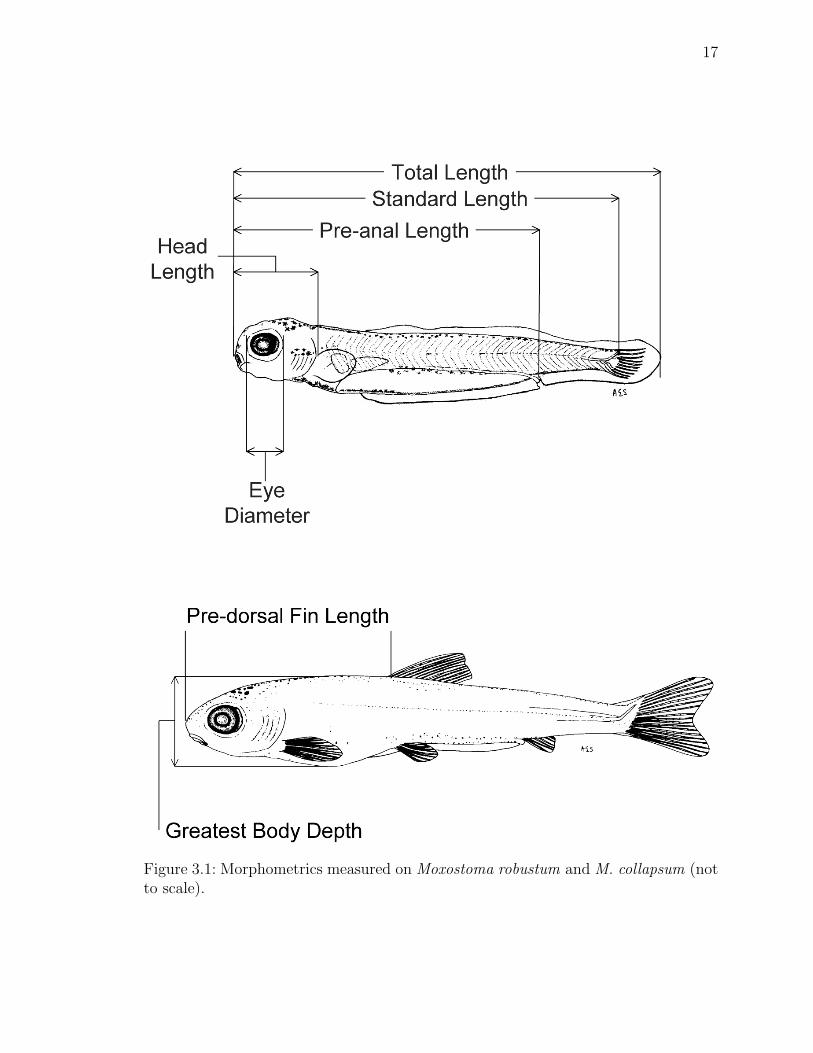
post-yolk-sac larvae), head length, and eye diameter (Figure 3.1). Morphometrics
were measured by an expert larval taxonomist (Robert Wallus of Murphy, North
Carolina) to ensure that operator error did not contribute to the observed
differences between the two species. Morphometrics were defined as follows (based
on Wallus et al. 1990):
Total length: Straight-line distance from the anterior-most part of the head to
the tip of the tail or caudal fin.
Standard length: Straight-line distance from the anterior-most part of head to
the most posterior point of the notochrod or hypural complex.
Pre-anal length: Distance from the anterior-most part of the head to the
posterior margin of the anus.
Pre-dorsal fin length: Distance from the anterior-most part of the head to the
anterior margin of the dorsal fin. Measured in larvae with dorsal fin
development.
Head length: Distance from the anterior-most tip of the head to the
posterior-most part of the opercular membrane, excluding the spine; prior to
opercular development, measured to the posterior end of the auditory vesicle.
Eye diameter: Horizontal measurement of the iris of the eye.
Greatest body depth: Greatest vertical depth of the body excluding fins and
finfolds. Measured on post yolk-sac larvae.
All measurements were at least to the nearest 0.1 mm, and some to the nearest 0.05
mm.
The expert taxonomist also provided qualitative narrative descriptions of the
developmental progress of each species (Appendices C and D). These narratives
17
Figure 3.1: Morphometrics measured on Moxostoma robustum and M. collapsum (notto scale).

18
were used as the basis for quantitative analysis of descriptive traits. Descriptive
traits measured included pigmentation patterns (observed with a polarized light
filter) and total length of fish at the time of certain ontogenetic events (such as yolk
absorption, finfold development, and the development of fins) (Table B.2).
Descriptive characters were scored as either present, absent, or undeveloped and
used in the statistical analysis. Several meristics (including myomere and fin ray
counts) were measured, but were not used for the statistical analysis because they
were found previously to be non-diagnostic (Looney and Jennings 2005). The
notchlip redhorse larvae used for data collection were archived in the Georgia
Museum of Natural History (accession number GMNH4434) for future reference.
Statistical Analysis and Key Creation
Quantitative measurements were tested for differences between the species by
overlaying plots of their relationship to total length in each species (PROC GPLOT,
SAS Institute) and looking for divergence between the two species. Chi-square tests
of association were used to test for significant (α=0.05) differences in the categorical
measurements between species (Snedecor and Cochran 1989). 14 traits were selected
based on a combination of ease-of-use and statistical significance for further
analysis. CATDAT, a computer program for categorical data analysis (Peterson et
al. 1999), was used to fit a classification tree model to the data.
TL was included in the tree model to explicitly incorporate the morphological
development that occurs as the fish grows. This approach obviates the need to make
a separate tree and key for each millimeter size class. The classification tree was
kept to 14 other traits (either qualitative or quantitative) because of technical
limitations of the CATDAT program.
CATDAT is capable of generating many different tree models based on user
specification of several variables, including tree size and size of each “partition”, or

19
subset, of the data (Peterson et al. 1999). The final model was chosen to minimize
both tree size (number of nodes) and the expected error rate (EER) of the model.
The EER of the model was estimated using leave-one-out cross validation, which
has been found to be an almost unbiased estimator of EER (Fukunaga and Kessel
1971). The key was checked for accuracy and ease-of-use by 3 independent verifiers
using laboratory-reared larval robust and notchlip redhorse of known identity. The
broodstock used to produce these larvae were collected at a different time than
those that produced the larvae used to create the model. Each verifier tested the key
on two samples of 25 larvae of each species, for a total of two replicates of 50 fishes.
The verifiers had a variety of experience using larval keys: one with less than 1 year
experience working with larval keys, one with 5 years of experience, and one with 20
years of experience. Their suggestions on improving clarity and ease-of-use were
incorporated into the key after they all completed both replicates of the verification.

Chapter 4
Results
Notchlip Redhorse Broodstock Collection and Spawning Induction
Twenty-nine notchlip redhorse were collected from various sites in the Oconee and
Broad Rivers. Of these, two (one male and one female) from the Broad River were
running ripe and were strip-spawned in the field, yielding approximately 2000
fertilized eggs. The remaining 27 were taken to the University of Georgia Whitehall
Fisheries Research lab for artificially-induced spawning.
Twenty notchlip redhorse (16 females and four males) were treated with
OvaprimTMto induce gonadal production. Seven (four females and three males)
responded to the treatment and reached spawning condition. However, the response
of the males and females was asynchronous, and fertilized eggs were not obtained.
Morphometrics
Morphometrics were measured on 68 notchlip redhorse larvae (hatched from the
Broad River-collected eggs) and 101 robust redhorse (hatched from Oconee
River-collected eggs). The size of the larvae ranged from 9.0–21.0 mm TL for
notchlip redhorse and 7.2–22.7 mm TL for robust redhorse. Of the morphometrics
measured (Figure 3.1), only pre-anal length as a percent of total length showed
divergence between the two species throughout the size range (Figures 4.1–4.6) and
was used in the classification tree. The remaining morphometrics showed either
little divergence or only diverged over a part of the size range of the larvae. These
characteristics were omitted from the classification tree model.
20

21
Figure 4.1: Standard length (expressed as % total length) in laboratory-reared larvalnotchlip redhorse (Moxostoma collapsum) and robust redhorse (M. robustum).
Figure 4.2: Pre-anal length (expressed as % total length) in laboratory-reared larvalnotchlip redhorse (Moxostoma collapsum) and robust redhorse (M. robustum).

22
Figure 4.3: Pre-dorsal fin length (expressed as % total length) in laboratory-rearedlarval notchlip redhorse (Moxostoma collapsum) and robust redhorse (M. robustum).
Figure 4.4: Greatest body depth (expressed as % total length) in laboratory-rearedlarval notchlip redhorse (Moxostoma collapsum) and robust redhorse (M. robustum).

23
Figure 4.5: Head length (expressed as % total length) in laboratory-reared larvalnotchlip redhorse (Moxostoma collapsum) and robust redhorse (M. robustum).
Figure 4.6: Eye diameter (expressed as % total length) in laboratory-reared larvalnotchlip redhorse (Moxostoma collapsum) and robust redhorse (M. robustum).

24
Table 4.1: Descriptive and ontogenetic traits used in the classification tree analysis.The size-class(es) for which the trait is significantly distinctive between the species islisted. A more detailed description of the traits appears in Table 4.2.
Character measured Size class (mm) p-value of χ2
Head position 10 < 0.001Head position 11 < 0.001Notochord flexion 10 < 0.001Notochord flexion 11 < 0.001Eye pigment 11 0.001Eye pigment 12 < 0.001Myosepta pigment 11 < 0.001Digestive tract 13 < 0.001Dorsal fin 13 < 0.001Yolk sac 14 < 0.001Dorsal fin margins 14 < 0.001Anal fin 14 < 0.001Anal fin 15 < 0.001Pelvic flaps 15 0.001Lip pigment 16 0.003Snout pigment 17-20 0.003
Descriptive Characters
Fifty-nine descriptive and ontogenetic traits were scored on 149 of the fishes (68
notchlip redhorse from the Broad River and 81 robust redhorse from the Oconee
River). Of the traits measured, 13 were selected for inclusion in the classification
tree analysis, with at least one significant difference between the two species selected
from each millimeter size-class (Tables 4.1 and 4.2). Total length and pre-anal
length also were included in the classification tree analysis.

25
Classification Tree Model
The classification tree models were fit to measurements of 149 fishes. The final
model was selected to minimize both tree size and expected error rate. The
classification tree chosen was a 24-node tree with 12 terminal nodes and 12
non-terminal nodes (Figures 4.7–4.8. The leave-one-out cross-validation expected
error rate was 4.7%. The prediction error rate for notchlip redhorse (i.e., the number
of fishes classified by the model as notchlip redhorse that were actually robust
redhorse) was 0%. The prediction error rate for robust redhorse was 7.95%. The
classification tree model was used to form the key found in Appendix A.
Key Validation
The key was tested by three independent testers in two replicates of 50 fishes (25 of
each species). The overall average accuracy rate for the three testers over two
replications was 95%. Tester A, who had approximately 20 years of experience
identifying larval fishes, correctly identified 48 of 50 fishes (96%) in each replication.
Tester B, with approximately five years of experience, correctly identified 47 of 50
fishes (94%) in the first replication and 48 of 50 fishes (96%) in the second
replication. Tester C, who had less than one year of experience, correctly identified
47 of 50 fishes (94%) in each replication. In the first replication, six of the eight
errors (75%) were notchlip redhorse misidentified as robust redhorse. All six
notchlip redhorse errors were the result of two specimens that were misidentified by
all three testers. The source of the misidentification (i.e., couplet) was not consistent
among testers. Testers B and C each uniquely misidentified one robust redhorse as a
notchlip redhorse. Although the couplet leading to the robust redhorse
misidentification was not consistent, each error was the result of a total length
measurement that was incongruent with proper identification of the specimen.

26
Figure 4.7: Classification tree for the identification of larval robust redhorse (Moxos-toma robustum) and notchlip redhorse (M. collapsum). Descriptions of the predictorsappears in Table 4.2. The diagram continues in Figure 4.8
Figure 4.8: Continuation of the classification tree for the identification of larval robustredhorse (Moxostoma robustum) and notchlip redhorse (M. collapsum). Descriptionsof the predictors appears in Table 4.2. The diagram begins in Figure 4.7

27
Table 4.2: Descriptive and ontogenetic traits used in the classification tree model.Traits were measured on fishes of all sizes. Traits were scored as the more advancedstate for all remaining size classes once the trait became present in all specimens in agiven size class. In cases where the trait has a more and less advanced state, the lessadvanced state is listed first.Character DescriptionHead position Curved: head curved against yolk sac
Lifted: head lifted away from yolk sacNotochord flexion Straight: tip of notochord not flexed
Flexed: tip of notochord flexedEye pigment Unpigmented: middle of eye yellowish or unpigmented
Pigmented: middle of eye with brown or black pigmentMyosepta pigment Unpigmented: pigment absent on median myosepta
Pigmented: dashed line of pigment along median myoseptaDigestive tract Not functional: digestive tract development incomplete
Functional: digestive tract fully developed and functionalDorsal fin Absent: dorsal fin and dorsal fin profile absent
Developing: developing dorsal fin or dorsal fin profile evidentYolk sac Present: yolk sac present
Absent: yolk sac completely absorbedDorsal fin margins Undefined: margins of dorsal fin undefined
Defined: anterior and posterior margins fin well-definedAnal fin Absent: anal fin absent; development has not begun
Developing: anal fin development has begunPelvic flaps Absent: pelvic fin development has not begun
Flaps: pelvic flaps developingLip pigment Absent: pigment absent on upper lip
Upper: pigment present on upper lipSnout pigment Absent: melanophores absent across snout
Bar: bar of small melanophores present across snout

28
In the second replication, four of the seven identification errors (57.1%) were
notchlip redhorse misidentified as robust redhorse. Three of the notchlip redhorse
errors were the result of a single specimen misidentified by all three testers. All
three testers misidentified the specimen at couplet 8 of the key (digestive tract
development). The remaining notchlip redhorse identification error was from a
specimen uniquely misidentified by tester C at couplet 2 (total length). Two of the
robust redhorse identification errors were the result of a single specimen
misidentified as a notchlip redhorse by testers A and C. Each of these errors were
made at couplet 3 (total length). The remaining robust redhorse identification error
was a specimen uniquely misidentified by tester B at couplet 9 (eye pigment).

Chapter 5
Discussion
Key Development and Strategic Approach
The classification tree model yielded a key that is effective at discriminating
between larval robust and notchlip redhorse from hatch to 20 mm total length (TL).
To my knowledge, it is the first key to successfully distinguish between sympatric
early-stage larval Moxostoma in the southern United States. Indeed, there have
been few successful keys made for larval Moxostoma in any region. Fuiman (1982)
successfully distinguished between larval golden redhorse (M. erythrurum) and
shorthead redhorse (M. macrolepidotum) in the Great Lakes region after an earlier
failed attempt using fishes from the Great Lakes and northern Atlantic Slope
drainages (Fuiman and Witman 1979). There have been other attempts (e.g., Bunt
and Cooke 2004) to distinguish between larval Moxostoma by comparing published
descriptions with an on-hand collection, but there hasn’t been a statistically-verified
key. This is also the first key to identify larval robust redhorse: such a feat wasn’t
even possible until the recent rediscovery of the species.
Assessing this key’s accuracy relative to previously published keys is difficult,
because most published keys provide minimal description of statistical methods
used and lack discussion of identification error rate. Fuiman (1979) is an exception;
his key for five northern Atlantic Ocean drainage catostomid species accurately
identified 82.6 to 100% of the species, depending on developmental stage. However,
Fuiman’s key does not attempt to identify any congeners, which is a more difficult
29

30
task. In light of this, the 95% “real world” accuracy rate achieved with the
newly-developed key is satisfactory.
The couplets in the key presented here are almost exclusively based on TL at
the occurrence of certain ontogenetic events. Ontogenetic timing is effective because
newly-hatched robust redhorse are 1–2 mm smaller in TL than newly-hatched
notchlip redhorse and are more ontogenetically advanced at a similar size. For
example, an 11 mm TL robust redhorse may be several weeks old, whereas a
notchlip of the same length may only be several days old. The robust redhorse
would have had more time to feed and grow than the notchlip and would have
reached a more advanced life stage.
Ontogenetic timing often is used in larval keys, but usually only in a few
couplets (e.g., several of the keys in Hogue, Jr. et al. 1976 and Kay et al. 1994) or in
combination with other characters (e.g., Fuiman 1982). This key is unusual in that
it attempts to distinguish between sympatric congeners that are very similar in
appearance. Since I was unable to find any easily measured meristic, morphometric,
or pigmentary traits that differed consistently as the larvae grew, I relied on
ontogenetic timing to keep the key as simple and user-friendly as possible and to
avoid the difficulties of a very complex key. Kay et al. (1994) faced a similar
conundrum trying to identify the larvae of catostomids in the Ohio River drainage
and made a similar choice.
The downside of using ontogenetic timing is that the effect of environmental
variation (temperature, current, dissolved oxygen, food supply, light regime, etc.) on
the development of the fishes is unclear. I tried to minimize the effect of these
unknown factors by choosing several different types of developmental characters
(pigment, internal organ, and fin development). My goal was to eliminate as much
error as possible from the entire fish identification process, not just from the model
used to make the key.

31
The alternative to relying on ontogenetic timing is to either give up and only
identify fishes to family or genus (e.g., Moxostoma in Kay et al. 1990) or to use very
complex and difficult-to-measure characters. Snyder and Muth (1990) used the
latter approach to identify six catostomid species, and the resulting key is
exceptional in both its thoroughness and complexity. Snyder and Muth’s (1990) key
has approximately 1000 couplets, identifying the fishes from hatch through early
juvenile stages with a variety of meristics, morphometrics, pigment descriptions, and
ontogenetic traits. Although Snyder and Muth (1990) do not provide a statistical
analysis of their key, the model is presumably accurate if used properly by an expert
taxonomist. I don’t believe that the key is appropriate for lay users, and it’s
complexity may even lead to a higher error rate because of confusion or improper
measurement. My goal was to eliminate as much error as possible from the entire
fish identification process, not just from the model used to make the key.
Several of the predictors used to fit the model to the data were not included in
the final classification tree. These traits include pre-anal length, notochord flexion,
dorsal fin development, pelvic fin development, lip pigmentation, and snout
pigmentation. These probably were left out of the model because they were
autocorrelated with other characters and therefore not predictive.
Accuracy of Identification Using The Larval Key
There are three major sources of potential error in identifying larval fishes: the
accuracy of the model used to make the key, the precision of the key users, and
variables associated with the fishes being identified. I attempted to minimize the
overall error of the identification process by creating a key that would limit the
error in each individual component.
The classification tree model had an expected error rate of 4.7%, which
compares favorably to previously published keys (e.g., Fuiman 1979). The model as

32
constructed is based on a relatively small sample of limited genetic diversity;
nonetheless, tests of the key performed on fishes of a wider genetic background
showed the model to be accurate, and should limit concerns about sample size.
There should be minimal identification error based on the key itself.
Larval keys often are plagued by difficult-to-measure characters or complex
counts that are nearly impossible to make consistently. A highly accurate key is
useless if the users can’t properly measured the diagnostic traits. Therefore, I
included ease-of-measurement in my criteria for selecting traits to minimize error
associated with the users or the key. The similarity of the error rate of the key
verifiers (5%) compared to the expected error rate of the model (4.7%) suggests that
these attempts were successful. Including internal characters or other very
complicated traits in the model may have made it more accurate or adaptable to
environmental variation, but the cost of the increased accuracy would have been a
substantial decrease in the user-friendliness of the key. I wanted to avoid creating a
key as complex as Snyder and Muth’s (1990), and was unwilling to trade a slightly
more accurate model for a much more difficult-to-use key.
Limiting error associated with the model and the key users should minimize the
impact of uncontrollable variables, such as the condition of the fishes being
identified, on the identification process. Larval fishes are fragile and difficult to
collect; those caught in the field may be in poor physical condition because of
damage that occurred during sampling. They also will have developed under
different environmental conditions than the larvae used to form the key. These
factors could lead to misidentification. The key has at least minimal plasticity,
however: the second-party verifiers successfully identified fishes raised in the lab
under differing sets of conditions. Any remaining questions about the keys accuracy
on wild-caught fishes will be cleared up in the near future, when wild-caught,
genetically-identified fishes will be used to test the key.
33
Limitations of the Key
The most important limitation of the key is the reliance on total length. Improper
measurement of TL may cause misidentification of the specimen in question.
Additionally, specimens that have immeasurable TL because of damage or deformity
cannot be reliably identified with this key.
Another important limitation is that the data used to make the key were
collected entirely from fishes preserved in 10% buffered formalin. Other
preservatives, such as ethanol, may cause differential shrinkage and invalidate the
key. A separate key may need to be developed for such fishes.
The scarcity of larvae of both species limited the scope of the key, which is
accurate only to approximately 20 mm TL. I decided to allocate the larvae to make
a key that was accurate over a smaller range rather than one that was less accurate
over a larger range.
The goal of the project was to create a key that would identify the fishes up to
their juvenile stage, at which point the shape of their lips should be diagnostic.
Neither robust nor notchlip redhorse has reached the juvenile stage by 20 mm TL,
which means there are larval stages that cannot be identified with this key.
Although the size of the fishes when the lips become diagnostic is unknown, I
hypothesize that it is somewhere in the 30–50 mm TL range. Thus, there is a gap of
approximately 10–30 mm TL in which the fishes cannot be identified without using
the genetic techniques devised by Wirgin et al. (2004). Based on the growth rate of
the notchlip redhorse in the lab, this gap probably represents approximately 30–90
days of growth and development time.
Even if the specific traits in this key are non-diagnostic in fishes over 20 mm TL,
the general theme, that robust redhorse are more developed than notchlip redhorse
at similar size, should remain valid. Robust redhorse consistently begin to develop
each fin at a smaller size than notchlip redhorse. By 20 mm TL, robust redhorse

34
have rudimentary anal fins, sometimes with rays, and notchlip redhorse’s anal fins
are minimally developed if they are developed at all. The anal fin should continue
developing more quickly in robust redhorse, gaining a full complement of rays and a
well-defined profile at a smaller TL than in notchlip redhorse. The other characters
in the key should converge either by 20 mm TL or soon after. Any key made to
diagnose fishes beyond 20 mm TL should consider anal fin development.
There needs to be further study into how well the key works on fishes from
outside of the drainage. The key has not been tested on fishes collected outside of
the Oconee River in middle Georgia, and there could be significant local variations
in the fishes outside of Georgia that render the key inaccurate for those drainages.
When this project was conceived, robust redhorse had not been rediscovered outside
of Georgia, and including fishes from other systems would have been out of the
scope of this research. The Robust Redhorse Conservation Committee has been very
successful in finding additional populations of robust redhorse in Georgia and the
Carolinas, and the key should be tested for accuracy in these other drainages.
There are also several other closely related catostomids throughout the robust
redhorse’s range, notably the striped jumprock (Scartomyzon rupiscartes) and the
undescribed Scartomyzon species informally known as the brassy jumprock. I was
unable to obtain larval jumprocks for this key. Including them in future keys would
be interesting and worthwhile.
G.B. Fairchild once said that keys are “made by people who don’t need them for
people who can’t use them” (Wilkerson and Strickman 1990). Although that’s not
entirely true, larval fish keys are not perfect. The sources of error are too common,
and identification can be as much an art as it is a science. I have attempted to make
this key as accurate as possible by controlling the error of the entire identification
process. Hopefully, with conscientious users and good samples, this key will be a
useful tool for future research.

Bibliography
Academy of Natural Sciences. 2004. History of the ichthyology department.
Available: www.acnatsci.org/research/biodiv/ichthyology.html#history
(November, 2004).
Atchley, W.R., G.T. Gasking, and D. Anderson. 1976. Statistical properties of
ratios. Systematic Zoology 21:137–148.
Barlow, G. W. 1961. Causes and significance of morphological variation in fishes.
Systematic Zoology 10:105–117.
Barrett, T. A. 1997. Hormone induced ovulation of robust redhorse (Moxostoma
robustum). Master’s thesis. The University of Georgia, Athens, Georgia.
Bolker, J. A., and C. R. Hill. 2000. Pigmentation development in hatchery-reared
flatfishes. Journal of Fish Biology 56:1029–1052.
Brieman, L., J. H. Friedman, R. A. Olshen, and C. J. Stone. 1984. Classification
and regression trees. Chapman and Hall, New York, New York.
Bryant, R. T., J.W. Evans, R. E. Jenkins, and B. J. Freeman. 1996. The mystery
fish. Southern Wildlife 1(2):26–35.
Bunt, C. M., and S. J. Cooke. 2004. Ontogeny of larval greater redhorse Moxostoma
valenciennesi. The American Midland Naturalist 151:93–100.
Cope, E. D. 1870. A partial synopsis of the fishes of the fresh waters of North
Carolina. Proceedings of the American Philosophical Society 11:448–495.
35

36
DeMeo, T. 2001. Report of the Robust Redhorse Conservation Committee Annual
Meeting. October 3–5, 2001, South Carolina Aquarium, Charleston, South
Carolina.
Dilts, E. W. 1999. Effects of fine sediment and gravel quality on survival to
emergence of larval robust redhorse Moxostoma robustum. Master’s thesis. The
University of Georgia, Athens, Georgia.
Edwards, M., and D. R. Morse. 1995. The potential for computer-aided
identification in biodiversity research. Trends in Ecology and Evolution
10:153–158.
Evans, J. W. 1994. A fishery survey of Oconee River between Sinclair Dam and
Dublin, Georgia. Georgia Department of Natural Resources, Wildlife Resources
Division. Final Report, Federal Aid Project F-33. Social Circle, Georgia.
Evans, J. W. 1996. Meeting Summary of the Robust Redhorse Conservation
Committee Annual Meeting. Wildlife Resources Division, Social Circle, GA.
Freeman B. J., C. A. Straight, J. R. Knight, and C. M. Storey. 2002. Evaluation of
robust redhorse (Moxostoma robustum) introduction into the Broad River, GA
spanning years 1995– 2001. Submitted to the Georgia Department of Natural
Resources, Social Circle, GA.
Fuiman, L. A. 1979. Descriptions and comparisons of catostomid fish larvae:
Northern Atlantic drainage species. Transactions of the American Fisheries
Society 108:560–603.
Fuiman, L.A. 1982. Family Catostomidae, suckers. Pages 345–435. In: N. A. Auer,
editor. Identification of larval fishes of the Great Lakes Basin with emphasis on
the Lake Michigan drainage. Special Publication 82-3, Great Lakes Fishery
Commission, Ann Arbor, Michigan.

37
Fuiman, L. A., and D. C. Witman. 1979. Descriptions and comparisons of
catostomid fish larvae: Catostomus catostomus and Moxostoma erythrurum.
Transactions of the American Fisheries Society 108:604–619.
Fukunaga, K., and D. Kessell. 1971. Estimation of classification error. IEEE
Transactions on Computers C-20:1521–1527.
Fulford, R., and D. A. Rutherford. 2000. Discrimination of larval Morone geometric
shape differences with landmark-based morphometrics. Copeia 2000: 965–972.
Harris, R.J. 1985. A primer of multivariate statistics, 2nd edition. Academic Press,
New York, New York.
Higginbotham, D. L., and C. A. Jennings. 1999. Growth and survival of juvenile
robust redhorse Moxostoma robustum fed three different commercial feeds. North
American Journal of Aquaculture 61:167–171.
Hogue Jr., J. J., R. Wallus, and L. Kay . 1976. Preliminary guide to the
identification of larval fishes in the Tennessee River. Tennessee Valley Authority,
Norris, Tennessee.
Hubbs, C. L., and K. F. Lagler. 1958. Fishes of the Great Lakes Region. University
of Michigan Press, Ann Arbor, Michigan.
Jackson, D.A. and K.M. Somers. 1991. The spectre of spurious correlations.
Oecologia 86:147–151.
Jenkins, R. E., and N. M. Burkhead. 1993. Freshwater fishes of Virginia. American
Fisheries Society, Bethesda, Maryland.
Jennings, C. A., B. J. Hess, J. Hilterman, and G. L. Looney. 2000. Population
dynamics of robust redhorse (Moxostoma robustum) in the Oconee River,

38
Georgia. Final Project Report - Research Work Order No. 52. Prepared for the
U.S. Geological Survey, Biological Resources Division. Reston, Virginia.
Jennings, C. A., J. L. Shelton, B. J. Freeman, and G. L. Looney. 1996. Culture
techniques and ecological studies of the robust redhorse moxostoma robustum.
Final Report to the Georgia Power Company, Environmental Laboratory,
Atlanta, GA.
Jolliffe, I.T. 1986. Principal component analysis. Springer-Verlag, New York.
Karjalainen, J., H. Helminen, A. Hirovonen, J. Sarvala, and M. Viljanen. 1992.
Identification of vendace (Coregonus albula(L.)) and whitefish (Coregonus
lavaretus) larvae by the counts of myomeres. Archiv fur Hydrobiologie
125:167–173.
Kay, L.K., R. Wallus, and B.L. Yeager. 1994. Reproductive biology and early life
history of fishes in the Ohio River drainage. Volume 2: Catostomidae. Tennessee
Valley Authority, Chattanooga, Tennessee.
Kendall, A. W., E. H. Ahlstrom, and H. G. Moser. 1984. Early life history stages of
fishes and their characters. Pages 11-22 in American Society of Ichthyologists and
Herpetologists Special Publication #1, Ontogeny and Systematics of Fishes. Allen
Press, Inc., Lawrence, Kansas.
Lachenbruch, P.A. 1975. Discriminant analyses. Hafner, New York, New York.
Libosvarsky, J. and Z. Kux. 1982. Multivariate analysis of five morphometric
characters in the genus Gobio. Folia Zoologica 31:83–92.
Lindsey, C. C. 1958. Modification of meristic characters by light duration in
kokanee (Oncorhynchus nerka). Copeia 1958:134–136.
39
Lindsey, C. C. 1962. Experimental study of meristic variation in a population of
threespine sticklebacks, Gasterosteus aculeatus. Canadian Journal of Zoology
40:271–312.
Lindstrom, D. P. 1999. Molecular species identification of newly hatched Hawaiian
amphidromous gobioid larvae. Marine Biotechnology 1:167–174.
Looney, G. L. and C. A. Jennings. 2005. Descriptions of larval and juvenile robust
redhorse Moxostoma robustum. Bulletin of the Alabama Museum of Natural
History 23:1–8.
McAllister, D.E., R. Murphy, and J. Morrison. 1978. The compleat minicomputer
cataloging and research system for a museum. Curator 21:63–91.
Mayden, R.L. and B. R. Kuhajda. 1996. Systematics, taxonomy, and conservation
status of the endangered Alabama sturgeon, Scaphirhyncus suttkusi Williams and
Clemmer (Actinopterygii, Acipenseridae). Copeia 1996:241–273.
Methven, D. A., and C. McGowan. 1998. Distinguishing small juvenile Atlantic cod
(Gadus morhua) from Greenland cod (Gadus ogac) by comparing meristic
characters and discriminant function analyses of morphometric data. Canadian
Journal of Zoology 76:1054–1062.
Packard, G.C, and T.J. Boardman. 1988. The misuse of ratios, indices, and
percentages in ecophysiological research. Physiological Zoology 61:1–9.
Peterson, J. T., Haas, T. C., and Lee, D. C. 1999. CATDAT–A program for
parametric and nonparametric categorical data analysis, User’s manual version
1.0. Annual report 1999 to Bonneville Power Administration, Portland, Oregon.
Available: coopunit.forestry.uga.edu/unit homepage/Peterson/Software/software
(December 2004)

40
Pimentel, R.A. 1979. Morphometrics: the multivariate analysis of biological data.
Kendall/Hunt Publishing Co., Dubuque, Iowa.
Prairie, Y.T, and D.F. Bird. 1989. Some misconceptions about the spurious
correlation problem in the ecological literature. Oecologia 81:285–289.
Rohlf, F. J., and L. F. Marcus. 1993. A revolution in morphometrics. Trends in
Ecology and Evolution 8:129–132.
Ruetz III, C. R. 1997. Swimming performance of larval and juvenile robust
redhorse: implications for recruitment in the Oconee River, Georgia. Master’s
thesis. The University of Georgia, Athens, Georgia.
Snedecor, G. W., and W. G. Cochran. 1989. Statistical methods, 8th edition. Iowa
State University Press, Ames, Iowa.
Snyder, D. E. 1983. Identification of catostomid larvae in Pyramid Lake and the
Truckee River, Nevada. Transactions of the American Fisheries Society
112:333–348.
Snyder, D. E. 2002. Pallid and shovelnose sturgeon larvae-morphological description
and identification. Journal of Applied Ichthyology 18:240–265.
Snyder, D. E., and R. T. Muth. 1990. Descriptions and identification of razorback,
flannelmouth, white, Utah, bluehead, and mountain sucker larvae and early
juveniles. Technical publication no. 38, Colorado Division of Wildlife, Fort
Collins, Colorado.
Sokal, R. R. and F. J. Rohlf. 1981. Biometry, 2nd edition.Freeman and Company,
New York.

41
Strauss, R. E., and C. E. Bond. 1990. Taxonomic methods: Morphology. Pages
109–140 in C. B. Schreck and P. B. Moyle, editors. Methods for fish biology.
American Fisheries Society, Bethesda, Maryland.
Tringali, M. D. , T. M. Bert, and S. Seyoum. 1999. Genetic identification of
centropomine fishes. Transactions of the American Fisheries Society 128:446–458.
Urho, L. 1996. Identification of perch (Perca fluviatilis), pikeperch (Stizostedion
lucioperca) and ruffe (Gymnocephalus cernuus) larvae. Annales Zoologici
33:659–667.
Van Velzen, J., N. Bouton, and R. Zandee. 1998. A procedure to extract
phylogenetic information from morphometric data. Netherlands Journal of
Zoology 48:305–322.
Wallus, R., T. P. Simon, and B. L. Yeager. 1990. Reproductive biology and early
life history of fishes in the Ohio River drainage. Volume 1: Acipenseridae through
Esocidae. Tennessee Valley Authority, Chattanooga, Tennessee.
Walsh, S. J., D. C. Haney, C. M. Timmerman, and R. M. Dorazio. 1998.
Physiological tolerances of juvenile robust redhorse, Moxostoma robustum:
conservation implications for an imperiled species, Environmental Biology of
Fishes 51:429–444.
Weigel, D. E., J. T. Peterson, and P. Spruell. 2002. A model using phenotypic
characteristics to detect introgressive hybridization in wild westslope cutthroat
trout and rainbow trout. Transactions of the American Fisheries Society
131:389–403.
Weyers, R. S. 2000. Growth and survival of larval robust redhorse and silver
redhorse (Catostomidae) exposed to pulsed, high-velocity water. Master’s thesis.
The University of Georgia, Athens, Georgia.
42
Wilkerson, R., and D. Strickman. 1990. Illustrated key to female anopheline
mosquitoes of Central America from Mexico to Western Panama. Journal of the
American Mosquito Control Association 6:7–34.
Wirgin, I. 2002. Stock structure and genetic diversity in the robust redhorse
(Moxostoma robustum) from Atlanta slope rivers. Report to Electric Power
Research Institute, Duke Power Company and Carolina Power and Light.
Wirgin, I., D. Currie, J. Stabile, and C. A. Jennings. 2004. Development and use of
a simple DNA test to distinguish larval redhorses (Moxostoma) species in the
Oconee River, Georgia. North American Journal of Fisheries Management
24:293–298.

Appendix A
Key for Identifying Larval Moxostoma in the Oconee River, Georgia
Note
The following is an identification key for the larvae of the Moxostoma species
suckers found in the Oconee River, Georgia: the robust redhorse, M. robustum, and
the notchlip redhorse, M. collapsum. The key does not identify larvae of either the
striped jumprock, Scartomyzon rupiscartes, or the undescribed Scartomyzon known
informally as the brassy jumprock, both of which may have a similar appearance to
the Moxostoma. The key is not separated by total length (TL), although total
length is used to help separate the fishes. The key covers fishes between 10 mm and
20 mm in total length.
Identification Key
1 Dorsal Fin Development
a. Dorsal fin not present or anterior and posterior margins not well-defined . . . . 2
b. Dorsal fin forming with anterior and posterior margins visible and
well-defined . . . . . . . . . . . . . . . . . . . . . . . . . . . . . . . . . . . . . . . . . . . . . . . . . . . . . . . . . . . . . . . 3
2(1) Total Length
a. Total length is less than 13.5 mm. . . . . . . . . . . . . . . . . . . . . . . . . . . . . . . . . . . . . . . . . . .4
b. Total length is greater than or equal to 13.5mm . . . . . . . . . . . . . . . . . . . . . . . . . . . . 5
43

44
3(1) Total Length
a. Total length is less than 15.0 mm . . . . . . . . . . . . . . . . . . . . . . . . . . . . . . . M. robustum
b. Total length is greater than or equal to 15.0mm . . . . . . . . . . . . . . . . . . . . . . . . . . . . 6
4(2) Head Position
a. Head is lifted away from yolk sac . . . . . . . . . . . . . . . . . . . . . . . . . . . . . . . . . . . . . . . . . . . 7
b. Head is curved around yolk sac . . . . . . . . . . . . . . . . . . . . . . . . . . . . . . . . M. collapsum
5(2) Total Length
a. Total length is less than 14.0 mm. . . . . . . . . . . . . . . . . . . . . . . . . . . . . . . . . . . . . . . . . . .8
b. Total length is greater than or equal to 14.0 mm . . . . . . . . . . . . . . . M. collapsum
6(3) Anal Fin Development
a. Anal fin development has begun, with rudimentary rays forming in some
specimens . . . . . . . . . . . . . . . . . . . . . . . . . . . . . . . . . . . . . . . . . . . . . . . . . . . . . . M. robustum
b. No obvious anal fin development . . . . . . . . . . . . . . . . . . . . . . . . . . . . . . . M. collapsum
7(4) Total Length
a. Total length is less than 12.0 mm . . . . . . . . . . . . . . . . . . . . . . . . . . . . . . . M. robustum
b. Total length is greater than or equal to 12.0 mm . . . . . . . . . . . . . . . . . . . . . . . . . . . 9
8(5) Digestive tract Development
a. Digestive tract developed and functional . . . . . . . . . . . . . . . . . . . . . . . . M. robustum
b. Digestive tract not functional . . . . . . . . . . . . . . . . . . . . . . . . . . . . . . . . . . M. collapsum
9(7) Eye Pigmentation

45
a. Middle of eye with dark brown or black pigment . . . . . . . . . . . . . . . M. collapsum
b. Middle of eye yellowish or lacking pigment . . . . . . . . . . . . . . . . . . . . . . . . . . . . . . . . 10
10(9) Total length
a. Total length less than 12.6 mm . . . . . . . . . . . . . . . . . . . . . . . . . . . . . . . . . M. robustum
b. Total length greater than or equal to 12.6 mm . . . . . . . . . . . . . . . . . . . . . . . . . . . . 11
11(10) Digestive tract Development
a. Digestive tract developed and functional . . . . . . . . . . . . . . . . . . . . . . . . M. robustum
b. Digestive tract not functional . . . . . . . . . . . . . . . . . . . . . . . . . . . . . . . . . . M. collapsum

Appendix B
Characters Measured for the Classification Tree
The following tables contain information on the ontogenetic characters measured to
form the key. The characters measured varied with each size class (10.0–10.9 mm,
11.0–11.9 mm, and so forth); once a character appeared in a single specimen of
either species in a size class, it was measured for all specimens in that and each
successive size class until it was present in all specimens of both species, at which
point it was scored as the more developmentally advanced state for all remaining
size classes.
Table B.1: Descriptive and ontogenetic traits measured on robust redhorse (Moxos-
toma robustum) and notchlip redhorse (M. collapsum). The size-class(es) for which
the trait was measured is listed. A more detailed description of the traits appears in
Table B.2
Character measured Size class (mm) p-value of χ2
Yolk shape 10 0.730
Yolk shape 11 < 0.001
Head position 10 0.001
Head position 11 < 0.001
Myomere development 10 0.001
Myomere development 11 0.003
Pectoral flaps 10 0.001
Continued on next page
46

47
Table B.1 — continued from previous page
Character measured Size class (mm) p-value of χ2
Notochord flexion 10 0.001
Notochord flexion 11 < 0.001
Eye pigment 10 0.001
Body pigment 10 0.251
Pectoral fins 11 0.001
Pectoral fins 12 < 0.001
Caudal fin 11 < 0.001
Ventral finfold 11 < 0.001
Ventral finfold 12 < 0.001
Middle of eye pigment 11 0.001
Middle of eye pigment 12 < 0.001
Head pigment 11 < 0.001
Myosepta pigment 11 < 0.001
Peduncle pigment 11 0.004
Yolk depth 12 < 0.001
Branchiostegals 12 0.001
Opercular flaps 12 0.004
Caudal fin rays 12 0.004
Caudal fin differentiation 12 0.004
Yolk sac pigment 12 0.111
Peduncle pigment II 12 0.162
Peduncle pigment II 13 0.001
Yolk depth II 13 < 0.001
Nares 13 < 0.001
Continued on next page

48
Table B.1 — continued from previous page
Character measured Size class (mm) p-value of χ2
Digestive tract 13 < 0.001
Caudal fin II 13 < 0.001
Urostyle 13 0.008
Dorsal fin 13 < 0.001
Ventral finfold II 13 < 0.001
Dorsum melanophores 13 < 0.001
Dorsum melanophores 14 0.934
Dorsum melanophores 15 0.640
Dorsum melanophores 16 0.399
Chin pigment 13 0.689
Chin pigment 14 0.197
Yolk sac 14 < 0.001
Mouth position 14 0.009
Pelvic fins 14 < 0.001
Dorsal fin margins 14 < 0.001
Dorsal finfold 14 < 0.001
Anal fin 14 < 0.001
Arrow-shaped pigment 14 0.004
Arrow-shaped pigment 15 0.273
Gut melanophores 14 0.007
Jaw pigment 14 0.668
Gill arch pigment 14 < 0.001
Mouth position II 15 0.020
Anal fin II 15 0.001
Continued on next page

49
Table B.1 — continued from previous page
Character measured Size class (mm) p-value of χ2
Pelvic flaps 15 0.001
Dorsal finfold II 15 0.001
Ventral finfold III 15 0.001
Operculum length 16 835
Operculum length 20 0.157
Pelvic fins 16 0.003
Lip pigment 16 0.003
Snout pigment 17–19 0.003
Jaw pigment II 16 0.003
Head profile 16 0.003
Dorsal fin profile 20 0.157
Anal fin III 20 0.003
Pelvic fins II 20 0.157
Dorsal finfold III 20 0.157
Squamation 20 0.0157
Scale pigment 20 0.0157
Dorsum melanophores II 20 0.0157

50
Table B.2: Description of traits measured on larval robust redhorse (Moxostoma
robustum) and notchlip redhorse (M. collapsum). Traits were measured on fishes of
all sizes. Traits were scored as the more advanced state for all remaining size classes
once the trait became present in all specimens in a given size class. In cases where
the trait has a more and less advanced state, the less advanced state is listed first.
Character Description
Yolk shape Bulbous: yolk sac bulbous anteriorly
Cylindrical: yolk sac cylindrical throughout
Head position Curved: head still curved
Lifted: head lifted away from yolk sac
Myomeres Ongoing: post-anal myomeres still developing
Complete: all post-anal myomeres fully developed
Pectoral flaps Absent: pectoral flaps absent
Present: pectoral flaps present
Notochord flexion Straight: tip of notochord not flexed
Flexed: tip of notochord flexed
Eye pigment Unpigmented: middle of eye yellowish or unpigmented
Pigmented: middle of eye with brown or black pigment
Body pigment Absent: body without any pigmentation
Present: some melanophores present on body
Pectoral fins Absent: pectoral flaps present or pectoral fins absent
Present: pectoral fins (not flaps) present
Caudal fin Undifferentiated: caudal fin undifferentiated from body
Differentiated: caudal fin differentiation has begun
Ventral finfold Absent: ventral finfold absent
Continued on next page

51
Table B.2 — continued from previous page
Character Description
Present: finfold present on posterior margin of yolk sac
Eye pigment II Absent: middle of eye unpigmented
Present: middle of eye with brown or black pigment
Head pigment Absent: Head pigment absent
Present: Pigment scattered on head over brain
Myosepta pigment Absent: pigment absent on median myosepta
Present: dashed line of pigment along median myosepta
Peduncle pigment Absent: caudal peduncle unpigmented
Present: Pigment scattered at base of caudal peduncle
Yolk depth Deep: yolk 2x deeper than torso
Shallow: yolk depth approximately equal to torso depth
Branchiostegals Absent: branchiostegals absent
Present: branchiostegal development is visible
Opercular flaps Absent: opercular flaps absent
Present: opercular flaps visible or forming
Caudal fin II Absent: caudal fin rays absent
Present: caudal fin rays present or forming
Caudal fin III Absent: caudal fin undifferentiated from body
Present: caudal fin obviously differentiated from body
Ventral finfold II Absent: ventral finfold absent anterior of yolk
Present: finfold present from yolk to pectoral fins
Yolk sac pigment Absent: yolk sac unpigmented
Present: pigment on dorsal margin of yolk sac
Peduncle pigment II Absent: caudal peduncle pigment sparse or light
Continued on next page

52
Table B.2 — continued from previous page
Character Description
Present: Dark pigment outlines caudal peduncle
Yolk depth II Deep: yolk depth greater than torso depth
Shallow: yolk depth less than torso depth
Nares Absent: nares absent
Present: nares visible
Digestive tract Functional: digestive tract fully developed
Not functional: digestive tract development incomplete
Caudal fin IV Unilobed: caudal fin unilobed
Bilobed: caudal fin bilobed
Urostyle Long: urostyle extends to dorsal margin of caudal fin
Short: urostyle stops before dorsal margin of caudal fin
Dorsal fin Absent: dorsal fin and fin profile absent
Developing: developing dorsal fin or fin profile evident
Ventral finfold III Absent: ventral finfold absent
Present: ventral finfold present
Dorsum pigment Present: 3–4 melanophores between eyes and pectorals
Absent: pigment absent between eyes and pectoral fins
Chin pigment Present: 2–3 melanophores present on chin
Absent: chin melanophores absent
Yolk sac Present: some yolk sac remaining
Absent: yolk sac fully absorbed
Mouth position Terminal: mouth terminal
Subterminal: mouth position ventral and subterminal
Pelvic fins Absent: pelvic fins and flaps absent
Continued on next page

53
Table B.2 — continued from previous page
Character Description
Present: pelvic fins or flaps present
Dorsal fin margins Undefined: margins of dorsal fin undefined
Defined: anterior and posterior margins well-defined
Dorsal finfold Continuous: finfold present throughout dorsum
Absorbed: finfold restricted to posterior half of dorsum
Anal fin Absent: anal fin absent; development has not begun
Present: anal fin development has begun
Arrow-shaped pigment Absent: pattern absent
Present: pattern present anterior to pectoral fin base
Gut melanophores Absent: melanophores absent on gut
Present: melanophores on gut posterior to air bladder
Jaw pigment Absent: pigment absent on jaw
Present: margin of jaw outlined in pigment
Gill arch pigment Absent: pigment absent on gill arches
Present: gill arches outlined in pigment
Mouth position II Oblique: mouth subterminal and oblique
Horizontal: mouth subterminal and horizontal
Anal fin II Early: anal fin absent or in nascent stages
Late: anal fin developing, possibly with rays
Pelvic flaps Absent: pelvic fin development has not begun
Flaps: pelvic flaps developed
Dorsal finfold II Present: significant portion of finfold still remains
Reduced: finfold greatly reduced or absent
Ventral finfold IV Present: significant portion of finfold still remains
Continued on next page

54
Table B.2 — continued from previous page
Character Description
Reduced: finfold greatly reduced or absent
Operculum length Short: operculum short of fin base
Long: operculum extends to fin base
Pelvic fins Short: fins short of margin of ventral finfold
Long: fins extend to margin of ventral finfold
Lip pigment Absent: pigment absent on upper lip
Upper: pigment present on upper lip
Snout pigment Absent: melanophores absent across snout
Bar: bar of small melanophores present across snout
Jaw pigment II Light: minimal or no pigment on jaw
Heavy: jaw outlined in heavy pigment
Head profile Flat: head profile flat posterior to eyes
Concave: head profile slightly concave posterior to eyes
Dorsal fin profile Straight: dorsal fin profile straight
Concave: dorsal fin profile concave
Anal fin III Early: fin without distinct profile and rays
Late: fin with distinct profile and 7–8 rays
Pelvic fins II Early: pelvic fins less developed, fewer than 7 rays
Developed: fins well-developed with at least 7 rays
Dorsal finfold III Present: finfold still remains
Absent: finfold entirely absorbed
Squamation Absent: squamation absent on caudal peduncle
Present: squamation visible on caudal peduncle
Scale pigment Absent: scales unpigmented
Continued on next page

55
Table B.2 — continued from previous page
Character Description
Present: pigment outlines scales from head to caudal fin
Dorsum pigment II Band: 3–4 melanophores from occiput to dorsal fin
None: band of melanophores absent

Appendix C
Development of Young Robust Redhorse
The following is a description of the development of larval and early juvenile robust
redhorse (Moxostoma robustum) based on a report prepared by Robert Wallus of
Murphy, North Carolina. This narrative is based on laboratory-reared specimens
from the Oconee River, Georgia and was used as the basis for the quantitative
analysis of the descriptive characters used in the model fitting (described in Chapter
3, Methods). Terminology is used as defined in Wallus et al. (1990).
Morphology
7.2–8.1 mm TL (newly hatched): Fish in this range have a yolk sac that is large and
bulbous (almost round) anteriorly. The head is small and slightly curved around the
anterior end of the bulbous portion of the yolk sac. Myomere development is
incomplete.
9.7–10.5 mm TL: The yolk material is visibly reduced and is cylindrical or
tubular throughout its length. The head has lifted away from the yolk. The
stomodeum is forming, but the mouth is not open.
11.2–11.7 mm TL: The yolk sac is still tubular, but it tapers in thickness
posteriorly. Yolk depth is greater than the depth of the torso. Internal head
development is visible; the mouth opening is apparent and gill arches are forming.
The heart is developing just anterior to the yolk sac.
56

57
12.2–12.9 mm TL: The yolk is reduced but still tubular, and is approximately as
deep as the torso. Branchiostegal formation has begun and opercular flaps are
forming.
13.0–14.0 mm TL: Opercular development continues until the opercular flap
covers the gills. Nares are visible and the otic chamber has formed. The head
appears flattened in profile and the eyes appear slightly flattened. The mouth is
subterminal and oblique. The digestive tract is functional on some individuals by
13.6 mm TL. The remaining yolk is still tubular at 13 mm TL and the depth of the
yolk is equal to about half the depth of the torso. The yolk is completely absorbed
son some individuals of 14.0 mm TL, but still present on others as large as 14.3 mm
TL.
14.3–16.0 mm TL: The head is flattened ventrally. The mouth is ventrally
located and progresses from subterminal and oblique to subterminal and horizontal.
The operculum is present to the base of the pectoral fins by 16 mm TL.
18.6–20.0 mm TL: Development continues and the dorsal head profile is now
slightly concave posterior to the eyes.
20.3 mm TL: Morphological development continues. Squamation is visible on
the caudal peduncle.
21.9–22.5 mm TL: Scalation is now visible mid-laterally on the body from the
caudal peduncle to the head.
Fin Development
72.–8.1 mm TL: The median finfold begins dorsally near the middle of the body
and extends posteriorly around the notochord, ending ventrally at the posterior
margin of the yolk sac. No other fin development is apparent.

58
9.7 mm TL: Pectoral flaps are present. The dorsal origin of the median finfold is
set back about 25% of TL from anterior edge of snout. The tip of the notochord is
slightly flexed.
11.2–11.7 mm TL: Notochord flexion is still slight. Caudal fin differentiation is
beginning: rays are unformed, but basal elements of the hypural complex are
forming. The developing pectoral fins are about 0.5 mm long. The dorsal origin of
the median finfold is now around myomeres 8–10; ventrally, the finfold is beginning
to form on the posterior margin of the yolk sac.
12.2–12.9 mm TL: Notochord flexion is more obvious and basal elements of the
caudal fin are well-formed. Incipient rays are forming in the caudal fin: 8–12 rays are
visible by 12.9 mm TL. The ventral finfold is now present anteriorly on the yolk sac
to about the position of the pectoral fins. The dorsal profile of the median finfold is
beginning to elevate at the future position of the dorsal fin.
13.6–14.3 mm TL: Pectoral fins are about 1.25 mm long. The caudal fin is
becoming bilobed with the urostyle extending to the dorsal margin of the caudal fin.
The dorsal fin profile is forming in the dorsal finfold, which is much reduced
anteriorly. Differentiation in the forming dorsal fin is obvious on some individuals by
13.8 mm TL. The anterior and posterior margins of the dorsal fin are nearly defined
between 14.0 and 14.3 mm TL and incipient rays are forming. The ventral finfold is
also decreasing in width and extends anteriorly to a position near the middle of the
abdominal cavity. Pelvic fins appear between 14.0 and 14.3 mm TL as narrow flaps
positioned ventro-laterally beneath the anterior half of the developing dorsal fin and
at the juncture of the gut and torso.
14.3–14.5 mm TL: The caudal fin is distinctly bilobed and well-developed, with
18 primary rays, some of which are segmented. The urostyle, positioned
immediately dorsal to the anterior-most primary caudal ray, still extends beyond
the hypural plate. The dorsal fin origin is around myomere 12 or 13, and the dorsal

59
fin has visible rays and well-defined anterior and posterior margins. The remainder
of the dorsal finfold is restricted between the dorsal fin and caudal fin, and is less
than half as deep as the torso. The ventral finfold is also reduced: it extends
anteriorly to the anus to near the pectoral fin bases at about the point of greatest
body depth. The anal fin is forming with pterygiophores (but no rays) present by
14.3 mm TL. The pectoral fins are about 1.5 mm long with visible rays.
15.2–15.9 mm TL: Anal fin rays are forming. There are 10–11 rays present in
the developing dorsal fin. The pelvic flaps are about half the width of the remaining
ventral finfold. The urostyle still extends past the hypural plate.
16.0–16.9 mm TL: The anal fin has a rounded margin, defined insertion, and
5–6 visible rays. The pelvic fins, with visible rays, extend to the margin of the
remaining ventral finfold. A small amount of dorsal finfold is still present between
the dorsal and caudal fins. The ventral finfold is present from the anus anteriorly to
about midway between the pectoral and pelvic find.
17.7–19.2 mm TL: No dorsal finfold remains. The ventral finfold is restricted to
the area between the pelvic fins and the anus. Fin development appears to be
nearing completion: all fins have well-developed rays and defined margins. The
urostyle still extends beyond the margin of the hypural plate. the dorsal fin profile
appears concave with at least 13 visible rays. The anal fin has 7–8 rays and eight or
more rays are visible in the pelvic fins. The pectoral fins are well-developed with at
leas 12–14 rays present.
20.0–22.5 mm TL: A very small remnant of finfold is present immediately
anterior to the anus at 20.3 mm TL. The finfold is completely gone and fin
development is complete, or nearly so, by about 22.5 mm TL.

60
Pigmentation
7.2–8.1 mm TL: The eyes, head, and body are all lacking pigment. The yolk is
yellowish in color.
9.7–10.5 mm TL: Eye pigment is becoming apparent. The only body pigment
consists of thin, dark dashes on some specimens along the median myosepta dorsal
to the yolk sac.
11.2–11.7 mm TL: The eyes are dark brown. Dorsally, pigment is scattered on
the head over the brain, narrowing on the occiput to a single mid-dorsal row on the
body to the origin of the dorsal finfold. Scattered melanophores are present dorsally
and ventrally at the base of the finfold on the caudal peduncle. Melanophores are
present mid-ventrally on the yolk sac from the base of the pectoral fins to the anus.
Lateral pigment consists of a dashed line along the median myosepta from the head
to about the middle of the caudal peduncle.
12.2–12.9 mm TL: The eyes are dark brown or black. The dorsal pigment
described above now consists of large, dark melanophores. Indistinct rows of small
melanophores appear on either side of the dorsal finfold in the middle of the body.
The pigment outlining the caudal peduncle is now darker. Internal pigment appears
scattered on the dorsal margin of the yolk sac.
13.0–14.3 mm TL: In addition to previously described pigment patterns,
melanophores are now present on the head around the tip of the snout at the
anterior margins of the nares. A few large melanophores are now scattered dorsally
on the head between the eyes. There are distinct lateral rows of pigment dorsally
over the middle of the body. These rows of pigments fuse posteriorly with dense,
scattered pigment on the caudal peduncle. A row of 3–4 melanophores is present
ventral to the otic chamber on the side of the head between the eyes and pectoral
fins. This row of pigment curves downward anteriorly from about the height of the
dorsal margin of the pectoral fin base. Ventral pigment on the yolk sac is now a

61
wide band of melanophores. Internally, the dorsal margin of the abdominal cavity is
covered with melanophores. Pigment is scattered on the caudal fin and at the base
of the caudal fin by 14.0–14.3 mm TL. Two to three melanophores are present on
the chin in some individuals.
14.3–15.9 mm TL: Ventral pigment is still heavy. There is an arrow-shaped
pigment pattern anterior to the pectoral base with its point near the isthmus. This
scattered pigment narrows at the base of the pectoral fins to a double row of
melanophores, which extend posteriorly to about the anterior margin of the ventral
finfold. Heavy pigment is scattered at the base of the finfold to the anus. Chin
pigment is present. Pigment outlines the gill arches. Pigment also is present on the
upper lip and snout. Internally, melanophores are scattered dorsally on the gut
posterior to the air chambers.
16.0–16.9 mm TL: Dorsally, uniformly scattered pigment covers the head,
occiput, and otic chamber. The large melanophores over the brain and in the single
row from the occiput to the dorsal fin origin are still present. Scattered small
melanophores cover the remainder of the dorsum. From the dorsal fin origin to the
middle of the caudal peduncle this pigment consists of scattered pigment between
dorso-lateral rows of small melanophores. From the middle of the caudal peduncle
to the base of the caudal fin this pigment consists of dark, densely scattered
pigment. Lateral pigmentation is little changed. Small melanophores are scattered
around the snout. The upper lip is pigmented on all specimens and small
melanophores are present on the lower lip in some specimens. Pigment is still visible
on the chin. There are fewer melanophores on the ventrum, especially on the gut
anterior to the developing pelvic fins. Dark, tightly scattered pigment is present on
the ventral caudal peduncle between the anal fin and the caudal fin. The arrow
pattern anterior to the pectoral fin bases is still present.

62
17.0–19.2 mm TL: Pigmentation in the form of small melanophores is beginning
to expand dorso-laterally. By 18.3 mm TL, little pigment is present ventrally
anterior to the pelvic fins, but there is still dark, tightly-scattered pigment posterior
to the pelvic fins along the gut and posterior to the anal fin. Small melanophores
are scattered throughout the caudal fin and on the anterior half of the dorsal fin.
Some pigment is present on the anal fin by 19.0 mm TL.
19.2–22.5 mm TL: The lateral progression of pigment is continuing. At 19.2 mm
TL, pigment is scattered laterally to just above the median myosepta. By 20.3 mm
TL, pigment has progressed slightly pas the median myosepta on sides of the body
anterior to the anal fin and small melanophores outline the scales on the caudal
peduncle. The scales are outlined in pigment from the caudal fin to the head on
individuals 21.9–22.5 mm TL.

Appendix D
Development of Young Notchlip Redhorse
The following is a description of the development of larval and early juvenile
notchlip redhorse (Moxostoma collapsum) based on a report prepared by Robert
Wallus of Murphy, North Carolina. This narrative is based on laboratory-reared
specimens from the Broad River, Georgia and was used as the basis for the
quantitative analysis of the descriptive characters used in the model fitting
(described in Chapter 3, Methods). Terminology is used as defined in Wallus et al.
(1990).
Morphology
9.0–9.3 mm TL (recently hatched): Yolk is bulbous anteriorly and cylindrical or
tubular posteriorly. Yolk is large: its greatest depth at least twice that of the torso.
Head is small and curved around the anterior margin of the yolk sac. Internal
development of the head is beginning: the developing brain and otic capsule are
visible. Post-anal myomeres are still developing.
10.5 mm TL: The head is lifting off the yolk, which is now bulbous anteriorly
and tubular behind.
11.2–11.9 mm TL: Yolk remains slightly bulbous anteriorly, otherwise tubular.
At 11.2 mm TL, the head is curved around the anterior margin of the yolk sac, but
by 11.9 mm TL the head has lifted and is on an axis nearly parallel to that of the
body. Head development continues with developing brain and otic capsule visible;
63

64
stomodeum development begins and the mouth is open on some specimens by 11.9
mm TL. Gill development begins. Post-anal myomere development continues.
12.1–12.7 mm TL: On most specimens the yolk is tubular throughout its length;
yolk depth is about twice that of torso. The head is on the same axis as the body.
Mouth opening may not have developed on all individuals but appears open at 12.7
mm TL. Developing gills are visible. By 12.7 mm TL, developing heart is apparent
just anterior to yolk and nasal openings are visible anterior to the eyes.
13.0–13.9 mm TL: Yolk remains tubular along its length, but absorption varies
with individual depth ranging from about equal to about twice that of the torso
(yolk depth was still about twice torso depth on an individual of 13.9 mm TL). Eyes
appear flattened. Gill development continues: opercular flap appears by 13.4 mm TL
and covers about half of the gill chamber by 13.8 mm TL. The mouth appears
subterminal and oblique by 13.9 mm TL.
14.0–14.9 mm TL: Yolk sac generally tubular along its length from gular region
to anus. Amount of yolk remaining ranges from about twice the depth of the torso
in an 14.2 mm TL individual to 14.1 mm TL individuals with very little yolk
remaining. Depth of yolk approximately to torso depth for a 14.7 mm TL
individual, so yolk may persist on larger specimens. However, all specimens greater
than 14.7 mm TL had completed yolk absorption. In summary, the yolk-sac phase of
these specimens is complete between about 14.2 and 14.8 mm TL. The last remnant
of remaining yolk is present just posterior to the air bladder. The gut appears above
the diminishing yolk; by 14.8 mm TL, the digestive tract is functional. The eyes still
appear slightly flattened. Development of the opercle, mouth, nasal openings, gills,
and heart is apparent. The opercle nearly covers the gill chamber on some
individuals by 14.0 mm TL and completely covers it on a 14.7 mm TL individual.
Branchiostegal development begins and is well-defined by 14.7 mm. Developing air
bladders are visible by 14.3 mm TL, their positions marked by concentrations of

65
pigment above them. Gill arches are evident by 14.3 mm TL and gills are
well-developed and visible by 14.7 mm TL. At 14.3 mm TL, the mouth is nearly
terminal and oblique with the lower lip at the level of the ventral margin of the eye;
however, a 14.9 mm TL individual’s mouth appeared subterminal and oblique.
15.1–15.6 mm TL: Internal development continues. Eyes appear flattened.
Mouth is subterminal and slightly oblique.
16.0–17.3 mm TL: Eyes appear slightly flattened. Mouth is subterminal, ventral,
and parallel to the body axis.
20.8–21.0 mm TL: Mouth is ventral and subterminal. Eyes appear round.
Fin Development
9.0–9.3 mm TL (recently hatched): The median finfold originates dorsally at a point
about 38% of TL and is present posteriorly around the notochord and ventrally to
the posterior margin of the yolk sac. No other fin development is apparent.
10.5 mm TL: The anterior dorsal finfold origin is at approximately 31% of TL.
11.2–11.9 mm TL: The finfold is little changed: it’s origin is at about 30% of TL
(around myomere 10–11). Pectoral fins visible as flaps by 11.3 mm TL.
12.1–12.7 mm TL: The dorsal origin of the finfold is at 30–34% of TL (myomere
10–11). The finfold becomes more visible on the posterior margin of the yolk sac.
The pectoral flaps are about 0.3 mm long at 12.1 mm TL.
13.0–13.9 mm TL: The dorsal finfold origin is at myomere 9–11, or about
1/4–1/3 of TL. As the yolk diminishes, the finfold becomes visible ventrally on the
yolk sac, extending anteriorly to the base of the pectoral fins by 13.7 mm TL.
Flexion begins; the urostyle moves dorsally to about a 45◦ angle by 13.9 mm TL.
Elements of the developing hypural plate are visible by 13.7 mm TL and caudal fin
ray development begins posterior to the upturned urostyle. 11–12 rudimentary rays
are visible in the caudal fin by 13.8 mm TL. An undulation in the dorsal finfold is

66
apparent in the area of the future dorsal fin. Pectoral fins are about 0.5 mm long at
13.9 mm TL.
14.0–14.9 mm TL: Fin development varies on individuals throughout this length
range. The dorsal finfold origin is usually at myomere 10 or 11. The occurrence of
the finfold ventrally on the yolk sac is variable and seems related to the amount of
yolk absorption. On a late yolk-sac larva (14.3 mm TL), the finfold was prominent
dorsally and ventrally, with its greatest depth dorsally above the anus and its
greatest depth ventrally between the anus and the posterior margin of the air
bladder. Dorsal fin develops with six pterygiophores and 3–4 rays visible by 14.9
mm TL. Pectoral fin growth and development also seems unrelated to TL. Rays
become visible as early as 14.3 mm TL. In this length range the length of the
pectoral fins varies from about 0.8 mm to about 1.75 mm. Tissue differentiation
becomes visible in the area of the future anal fin by 14.7 mm TL.
Caudal fin development also varies, but it progresses throughout the size range.
Flexion is obvious on most individuals, but hypural development and formation of
caudal fin rays varies without relation to TL. An 14.5 mm TL individual had no
visible caudal fin rays, while a late yolk-sac larva (14.1 mm TL) had 14–16
segmented rays. Flexion exceeded 45% on a 14.4 mm individual, but there was
minimal caudal fin development. By 14.9 mm TL, 16–18 segmented caudal fin rays
are visible, and hypural elements are well-defined. During caudal fin development,
the shape of the fin varies, progressing from a pointed finfold to a rounded tail that
widens posteriorly late in the yolk-sac phase and finally appears squared-off
posteriorly with visible lobes (at 14.9 mm TL). At 14.9 mm TL, the tip of the
urostyle extends beyond the dorsal profile of the torso.
15.1–15.6 mm TL: Finfold is little changed. The caudal fin appears squared-off
with obvious dorsal and ventral lobes; 15–17 segmented rays are present, and
hypural development is well defined. The tip of the urostyle still extends past the
67
dorsal profile of the torso. At 15.6 mm TL, the dorsal fin has eight pterygiophores
and seven visible rays, and is elevated to a point at the tip of its longest ray.
16.0–16.5 mm TL: Notches form in the finfold at several places: the posterior
margin of the developing dorsal fin, between the dorsal finfold and the caudal fin,
and at the posterior margin of the future anal fin. Caudal fin development varies: a
16.0 mm TL individual had advanced caudal development (17–18 segmented rays
and a bilobed appearance), but a 16.5 mm TL specimen ad only 13 segmented rays
and a rounded fin profile with no apparent lobes. The dorsal fin profile is pointed at
the tip of its longest ray with as many as 10–11 pterygiophores and rays visible.
Anal fin margins become defined and rudimentary rays form. The pelvic fins appear
as ventro-lateral flaps on the body below the middle of the dorsal fin.
17.1–17.3 mm TL: The finfold now has clearly defined notches at the posterior
margin of the dorsal fin, between the dorsal finfold and the caudal fin, and at the
posterior margin of the anal fin. At 17.3 mm TL, the caudal fin is bilobed and
almost completely developed, with 18 segmented rays and 3–4 secondary rays. The
tip of the urostyle is no longer visible above the dorsal profile of the torso. The
dorsal fin had 13 pterygiophores and 11–12 rays. Three pterygiophores and 3–4 rays
are visible in the developing anal fin. The pelvic flaps, positioned at the posterior
margin of the air bladder, are about 1/2 the depth of the ventral finfold.
20.8 mm TL: The finfold is greatly reduced dorsally and ventrally: a dorsal
remnant is barely visible between the dorsal and caudal fins and the ventral
remnant is present from anterior to the pelvic fins posterior to the anus; ventrally,
the finfold is completely absent between the anus and the caudal fin. The caudal fin
is bilobed with 18 segmented rays and 7–8 secondary rays. The posterior margin of
the anal fin is defined with 8 pterygiophores and 7 rays visible. The pectoral fins are
well-developed with at least 12 rays. The dorsal fin has 14 rays. Pelvic fins are about
1.25 mm long and extend past the margin of the ventral finfold with 6–7 visible rays.
68
17.7 mm SL (21.0+ mm TL: The only remaining remnant of the finfold is
present ventrally between the pelvic fins and the anus. Fin development for all fins
in nearly complete. Fin rays are as follows: the pectoral fins have 11–12 rays, the
anal fin has 7, the dorsal fin has 14, and the pelvic fins have 6–7 rays. The distal half
of this specimen’s caudal fin was missing, but its development appears complete.
Pigmentation
9.0–10.5 mm TL: The head and body lack pigment. The middle of the eye and the
yolk are yellowish.
11.2–11.9 mm TL: At 11.2 mm TL, the body and the head are unpigmented and
the middle of the eye and yolk are still yellowish. By 11.9 mm TL, the eyes are
developing pigment. Dorsal pigment is limited to a few melanophores in a row
anterior to the finfold origin. There is an irregular row of melanophores laterally
along the median myosepta from the head to the posterior margin of the yolk sac.
There is pigment scattered mind-ventrally on the yolk sac.
12.1–12.7 mm TL: The eyes become dark. At 12.2 mm TL, a few melanophores
are present over the hindbrain and occiput. Two large melanophores are present
mid-dorsally between the occiput and the dorsal finfold origin. Pigment is scattered
mid-ventrally on the yolk and a row of melanophores is present along the median
myosepta from the head to mid-body.
By 12.7 mm TL, there are many scattered melanophores on the dorsum from the
head above the eyes to the occiput. Along the body, pigment is scattered
mid-dorsally, near the base of the finfold, almost to the end of the urostyle. Ventral
pigment is concentrated on the yolk and along the base of the finfold onto the
caudal peduncle. Mid-lateral pigment is present along the median myosepta form
the pectoral fin flaps posteriorly to the mid caudal peduncle. Internal pigment if

69
visible in the gular region over the developing heart and along the ventral margin of
the abdominal cavity over the yolk.
13.0–13.9 mm TL: The eye is fully pigmented. Pigmentation patterns are
basically as described above with a few advancements. Dorsally, large melanophores
cover the head from the middle of the eyes to over the occiput. Pigment becomes
densely concentrated dorsally and ventrally along the caudal peduncle. Some
melanophores are visible around the tip of the urostyle. The mid-lateral row of
pigment now consists of 1–2 melanophores on each myomere. Ventral pigment on
the yolk appears as two rows of large melanophores positioned mid-ventrally.
Pigment appears on the tip of the snout. Internal pigment over the yolk expands
anteriorly, forming a broad patch of pigment over the area of the future air bladder.
Some pigment cells are scattered dorso-laterally along the yolk sac. Scattered
melanophores appear laterally on the developing hypural complex and in the region
of the developing caudal fin rays (the latter is only visible with a polarized light
filter).
14.0–14.9 mm TL: The pigment patterns described above progress with the
following observations. The tip of the snout becomes covered with a concentration
of small melanophores (which appear as a bar of pigment across the snout) and the
margin of the upper jaw becomes outlined in pigment. Dorsally, large melanophores
are present on the head between the eyes, over the brain, between the otic
chambers, and over the occiput. On the body, a mid-dorsal row of pigment is
flanked by irregular rows of melanophores, which gives the appearance of three rows
along the back. Pigment is lacking mid-dorsally only in the region of the developing
dorsal fin. Posterior to the anus, melanophores are smaller, concentrated across the
dorsum, and extended posteriorly almost to the urostyle. Similar dense pigment is
present ventrally behind the anus. Viewed laterally, these heavy concentrations of
pigment, dorsally and ventrally, outline the caudal peduncle.

70
There is a row of 2–4 melanophores parallel to the body axis on the chin. The
developing branchiostegals have a few small melanophores scattered on them. The
ventral gular pigment consists of scattered melanophores that are present from the
base of the pectoral fins to a point at the isthmus. A mid-ventral row of 5–6 pairs of
large melanophores extends posteriorly from the base of the pectoral fins and joins a
single row of large melanophores that extends to the anus. This row of pigment,
posterior to the pairs of melanophores, is usually a single row. However, more than
one melanophore may be present mid-ventrally on some individuals.
Laterally, the most obvious body pigment is restricted to the single row of small
melanophores (2–4 per myomere) that extends from the pectoral fins onto the
caudal peduncle. Some scattered pigment is present on the developing hypural
complex, caudal fin, and on the urostyle near the tip. A few small melanophores are
present on the side of the head, lateral to the otic chamber and on the opercle.
Internally, 3–4 melanophores appear in a diagonal row at the base of the
pectoral fins. The gill arches become outlined with pigment. Large melanophores are
scattered over the developing stomach, behind the eyes, and under the brain. Dense
pigmentation covers the developing air bladders and extends posteriorly along the
ventral surface of the abdominal cavity and along the dorsal surface of the gut.
15.1–15.6 mm TL: Pigment is as above with a few advancements. Laterally,
about midway between dorsal pigment and the mid-lateral stripe is an internal row
of small melanophores that extends from the posterior margin of the hindbrain to
the upturned urostyle. By 15.6 mm TL, a few scattered melanophores are present
ventro-laterally along the posterior 1/3 of the gut.
16.0–16.5 mm TL: Pigment is as above with a few advancements. On the body,
pigment becomes scattered across the entire dorsal surface except mid-dorsally
under the developing dorsal fin. Some melanophores are slightly dorso-lateral in
position. Dorsal head pigment between the eyes extends anteriorly to the bar of

71
pigment across the snout. Scattered pigment increases on the head laterally and
ventrally.
17.1–17.3 mm TL: Pigment is generally the same as above. External lateral
pigment is present on the stomach and air bladders.
20.8 mm TL–17.7 mm SL: Pigment is as above with several additions. Dorsal
pigment starts at the mouth and is prominent over the snout onto the head. The
head is covered with pigment dorsally and dorso-laterally to about the middle of the
eyes. A band of pigment 3–4 cells across extends mid-dorsally from the occiput
pigment to the dorsal fin origin. A double row of pigment is present mid-dorsally
from the dorsal fin insertion to the caudal fin. Scattered pigment is present
dorso-laterally throughout the body. Pigment is scattered laterally along the sides of
the stomach, air bladders, and gut. Small melanophores are scattered ventrally on
the head and under the eyes. Gill arches are still outlined with pigment.
Melanophores are present along the margins of most dorsal fin rays and blotches of
pigment are present on the membranes between the rays at the distal margin of the
fin. Melanophores also outline caudal fin rays and a few are present in the anal fin.

Appendix E
Morphometric and Descriptive Measurements
The following table contains all of the measurements used to fit the classification
tree model. All measurements were made using a stereo dissecting microscope at
10x magnification. Morphometrics were measured as described in Chapter 3
(Methods). An explanation of the descriptive characters can be found in Table B.2.
72
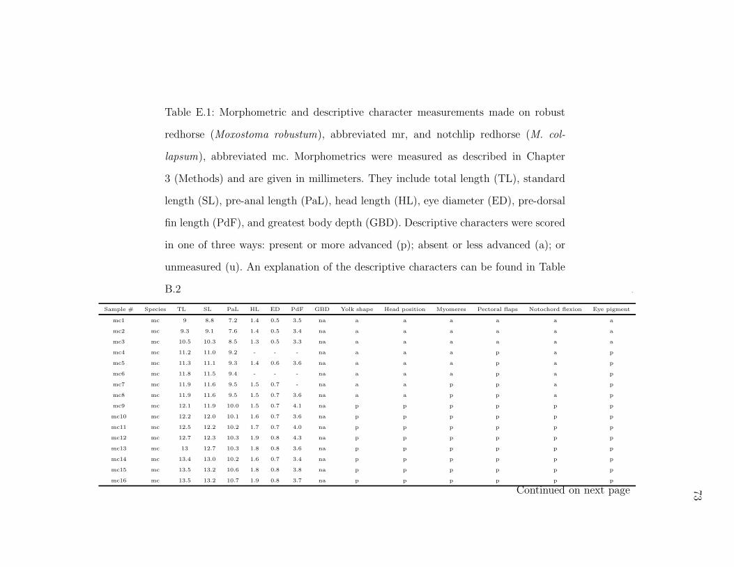
73
Table E.1: Morphometric and descriptive character measurements made on robust
redhorse (Moxostoma robustum), abbreviated mr, and notchlip redhorse (M. col-
lapsum), abbreviated mc. Morphometrics were measured as described in Chapter
3 (Methods) and are given in millimeters. They include total length (TL), standard
length (SL), pre-anal length (PaL), head length (HL), eye diameter (ED), pre-dorsal
fin length (PdF), and greatest body depth (GBD). Descriptive characters were scored
in one of three ways: present or more advanced (p); absent or less advanced (a); or
unmeasured (u). An explanation of the descriptive characters can be found in Table
B.2 .
Sample # Species TL SL PaL HL ED PdF GBD Yolk shape Head position Myomeres Pectoral flaps Notochord flexion Eye pigment
mc1 mc 9 8.8 7.2 1.4 0.5 3.5 na a a a a a a
mc2 mc 9.3 9.1 7.6 1.4 0.5 3.4 na a a a a a a
mc3 mc 10.5 10.3 8.5 1.3 0.5 3.3 na a a a a a a
mc4 mc 11.2 11.0 9.2 - - - na a a a p a p
mc5 mc 11.3 11.1 9.3 1.4 0.6 3.6 na a a a p a p
mc6 mc 11.8 11.5 9.4 - - - na a a a p a p
mc7 mc 11.9 11.6 9.5 1.5 0.7 - na a a p p a p
mc8 mc 11.9 11.6 9.5 1.5 0.7 3.6 na a a p p a p
mc9 mc 12.1 11.9 10.0 1.5 0.7 4.1 na p p p p p p
mc10 mc 12.2 12.0 10.1 1.6 0.7 3.6 na p p p p p p
mc11 mc 12.5 12.2 10.2 1.7 0.7 4.0 na p p p p p p
mc12 mc 12.7 12.3 10.3 1.9 0.8 4.3 na p p p p p p
mc13 mc 13 12.7 10.3 1.8 0.8 3.6 na p p p p p p
mc14 mc 13.4 13.0 10.2 1.6 0.7 3.4 na p p p p p p
mc15 mc 13.5 13.2 10.6 1.8 0.8 3.8 na p p p p p p
mc16 mc 13.5 13.2 10.7 1.9 0.8 3.7 na p p p p p p
Continued on next page

74
Table E.1 — continued from previous pageSample # Species TL SL PaL HL ED PdF GBD Yolk shape Head position Myomeres Pectoral flaps Notochord flexion Eye pigment
mc17 mc 13.5 13.1 10.7 1.8 0.8 4.3 na p p p p p p
mc18 mc 13.7 13.2 10.8 1.8 0.8 4.0 na p p p p p p
mc19 mc 13.7 13.2 10.1 2.1 0.8 4.5 na p p p p p p
mc20 mc 13.7 13.1 10.1 2.1 0.8 4.2 na p p p p p p
mc21 mc 13.8 13.4 10.7 1.8 0.9 4.3 na p p p p p p
mc22 mc 13.8 13.1 10.2 2.1 0.9 4.5 na p p p p p p
mc23 mc 13.8 13.0 10.0 2.3 0.8 4.6 na p p p p p p
mc24 mc 13.9 13.5 10.6 1.9 0.8 4.3 na p p p p p p
mc25 mc 13.9 13.3 10.2 2.0 0.9 4.5 na p p p p p p
mc26 mc 13.9 13.2 10.4 2.1 0.8 4.6 na p p p p p p
mc27 mc 14 13.5 10.8 1.8 0.8 4.3 na p p p p p p
mc28 mc 14 13.3 10.6 2.0 0.9 4.8 na p p p p p p
mc29 mc 14 13.4 10.2 2.2 0.9 4.6 na p p p p p p
mc30 mc 14.1 13.8 11.1 1.9 0.8 4.0 na p p p p p p
mc31 mc 14.1 13.3 10.1 2.6 1.0 5.6 na p p p p p p
mc32 mc 14.1 13.2 10.2 2.5 1.0 - na p p p p p p
mc33 mc 14.2 13.8 11.1 1.8 0.8 4.2 na p p p p p p
mc34 mc 14.2 13.8 11.1 1.8 0.8 4.2 na p p p p p p
mc35 mc 14.2 13.8 11.0 1.9 0.8 4.0 na p p p p p p
mc36 mc 14.2 13.4 10.4 2.1 0.8 4.6 na p p p p p p
mc37 mc 14.2 13.7 10.7 2.2 0.9 4.6 na p p p p p p
mc38 mc 14.2 13.6 10.8 2.2 0.9 4.2 na p p p p p p
mc39 mc 14.2 13.3 10.3 2.4 0.9 4.6 na p p p p p p
mc40 mc 14.2 13.5 10.5 2.1 0.9 4.9 na p p p p p p
mc41 mc 14.3 13.5 10.4 2.2 0.8 4.7 na p p p p p p
mc42 mc 14.3 13.2 10.1 2.1 0.9 4.5 na p p p p p p
mc43 mc 14.3 13.8 10.5 2.4 1.0 4.7 na p p p p p p
mc44 mc 14.3 13.7 10.6 2.5 1.0 5.0 na p p p p p p
mc45 mc 14.4 13.8 10.7 2.3 0.9 4.7 na p p p p p p
mc46 mc 14.4 13.7 10.7 2.2 0.9 4.4 na p p p p p p
mc47 mc 14.5 13.9 10.8 2.4 0.8 4.7 na p p p p p p
mc48 mc 14.5 13.5 10.4 2.3 0.9 4.8 na p p p p p p
mc49 mc 14.6 14.0 11.0 2.2 0.9 4.7 na p p p p p p
mc50 mc 14.6 14.0 10.8 2.3 0.9 4.5 na p p p p p p
Continued on next page

75
Table E.1 — continued from previous pageSample # Species TL SL PaL HL ED PdF GBD Yolk shape Head position Myomeres Pectoral flaps Notochord flexion Eye pigment
mc51 mc 14.6 13.7 10.7 2.4 0.9 4.8 na p p p p p p
mc52 mc 14.6 13.9 10.7 2.6 1.0 5.0 na p p p p p p
mc53 mc 14.7 14.0 11.0 2.3 0.9 4.7 na p p p p p p
mc54 mc 14.7 13.7 10.5 2.4 1.0 4.9 na p p p p p p
mc55 mc 14.7 13.4 10.5 2.2 0.9 4.7 na p p p p p p
mc56 mc 14.7 13.9 10.6 2.3 0.9 4.8 na p p p p p p
mc57 mc 14.7 13.9 10.8 2.7 0.9 5.5 na p p p p p p
mc58 mc 14.8 13.5 10.6 2.5 1.0 5.0 na p p p p p p
mc59 mc 14.9 13.3 10.5 2.5 1.0 4.9 na p p p p p p
mc60 mc 15.1 13.5 10.6 2.5 1.0 5.4 - p p p p p p
mc61 mc 15.6 13.9 11.0 2.7 1.1 5.3 - p p p p p p
mc62 mc 16 14.1 11.3 2.9 1.1 5.5 - p p p p p p
mc63 mc 16.1 14.1 11.2 3.0 1.1 5.4 - p p p p p p
mc64 mc 16.5 14.5 11.3 2.9 1.1 6.5 - p p p p p p
mc65 mc 17.1 14.8 11.8 3.1 1.2 6.2 - p p p p p p
mc66 mc 17.3 14.7 11.9 3.0 1.2 6.3 - p p p p p p
mc67 mc 20.8 17.5 13.8 4.1 1.3 6.4 - p p p p p p
mc68 mc 21 17.7 13.7 4.4 1.5 7.8 - p p p p p p
mr1 mr 10 9.6 7.8 1.3 0.5 2.7 na p p p p p p
mr2 mr 10 9.6 7.9 1.3 0.6 2.6 na p p p p p p
mr3 mr 10.05 9.7 8.0 1.3 0.6 2.4 na p p p p p p
mr4 mr 10.3 10.0 8.1 1.2 0.5 2.7 na p p p p p p
mr5 mr 10.4 10.1 8.2 1.3 0.5 2.8 na p p p p p p
mr6 mr 10.7 10.4 8.6 1.4 0.5 2.9 na a p p p p p
mr7 mr 10.7 10.3 8.5 1.4 0.6 2.8 na a p p p p p
mr8 mr 10.8 10.4 8.6 1.4 0.6 2.6 na p p p p p p
mr9 mr 10.8 10.4 8.5 1.4 0.6 2.6 na p p p p p p
mr10 mr 10.9 10.5 8.7 1.4 0.5 2.7 na a p p p p p
mr11 mr 11.2 10.6 8.6 1.6 0.6 3.0 na p p p p u p
mr12 mr 11.3 10.8 8.6 1.5 0.6 3.0 na p p p p p p
mr13 mr 11.3 10.8 8.6 1.6 0.6 2.9 na p p p p p p
mr14 mr 11.6 11.1 8.9 1.6 0.6 3.0 na p p p p p p
mr15 mr 11.6 11.0 8.9 1.7 0.6 3.1 na p p p p p p
mr16 mr 11.6 11.0 8.9 1.7 0.6 3.1 na p p p p u p
Continued on next page

76
Table E.1 — continued from previous pageSample # Species TL SL PaL HL ED PdF GBD Yolk shape Head position Myomeres Pectoral flaps Notochord flexion Eye pigment
mr17 mr 11.7 11.2 8.9 1.6 0.7 3.1 na p p p p p p
mr18 mr 11.7 11.2 8.9 1.7 0.7 3.0 na p p p p u p
mr19 mr 11.9 11.5 9.1 1.7 0.7 3.1 na p p p p p p
mr20 mr 11.9 11.3 9.0 1.6 0.7 3.2 na p p p p p p
mr21 mr 11.9 11.4 9.2 1.7 0.7 3.1 na p p p p p p
mr22 mr 11.9 11.4 8.9 1.7 0.7 3.1 na p p p p p p
mr23 mr 12 11.4 9.1 2.1 0.8 3.5 na p p p p p p
mr24 mr 12.1 11.4 9.1 1.7 0.7 3.1 na p p p p p p
mr25 mr 12.2 11.5 9.0 1.7 0.8 3.3 na p p p p p p
mr26 mr 12.2 11.7 9.0 1.8 0.8 3.3 na p p p p p p
mr27 mr 12.2 11.5 9.1 1.8 0.7 3.4 na p p p p p p
mr28 mr 12.2 11.5 9.0 2.1 0.8 3.6 na p p p p p p
mr29 mr 12.2 11.6 9.2 2.1 0.8 3.5 na p p p p p p
mr30 mr 12.3 11.7 9.2 1.8 0.8 3.5 na p p p p p p
mr31 mr 12.4 11.8 9.4 1.7 0.8 3.3 na p p p p p p
mr32 mr 12.5 11.8 9.4 2.1 0.7 3.7 na p p p p p p
mr33 mr 12.6 11.9 9.6 1.8 0.7 3.5 na p p p p p p
mr34 mr 13 12.2 9.1 2.2 0.8 4.2 na p p p p p p
mr35 mr 13 12.2 9.3 2.1 0.9 4.0 na p p p p p p
mr36 mr 13.1 12.4 9.6 2.0 0.8 3.7 na p p p p p p
mr37 mr 13.3 12.8 9.6 2.0 0.8 4.3 na p p p p p p
mr38 mr 13.3 12.6 9.8 2.2 0.8 4.0 na p p p p p p
mr39 mr 13.3 12.6 9.4 2.1 0.9 4.2 na p p p p p p
mr40 mr 13.4 12.6 9.2 2.0 0.8 4.0 na p p p p p p
mr41 mr 13.6 13.1 9.8 2.1 0.8 4.4 na p p p p p p
mr42 mr 13.7 13.1 9.6 2.2 0.9 4.2 na p p p p p p
mr43 mr 13.9 13.0 9.8 2.1 0.9 4.0 na p p p p p p
mr44 mr 14 13.0 9.7 2.3 1.0 5.2 na p p p p p p
mr45 mr 14.1 12.6 9.5 2.6 1.0 5.2 na p p p p p p
mr46 mr 14.3 13.6 10.1 2.3 1.0 4.5 na p p p p p p
mr47 mr 14.3 12.8 9.7 2.5 1.0 5.3 na p p p p p p
mr48 mr 14.4 13.6 10.3 2.4 0.9 4.6 na p p p p p p
mr49 mr 14.4 13.7 10.1 2.3 0.9 4.4 na p p p p p p
mr50 mr 14.7 13.7 10.3 2.3 0.9 5.6 na p p p p p p
Continued on next page

77
Table E.1 — continued from previous pageSample # Species TL SL PaL HL ED PdF GBD Yolk shape Head position Myomeres Pectoral flaps Notochord flexion Eye pigment
mr51 mr 14.8 12.8 10.0 2.8 1.0 5.5 na p p p p p p
mr52 mr 14.9 13.3 10.1 2.6 1.0 5.5 na p p p p p p
mr53 mr 14.9 13.4 10.1 2.6 1.0 5.4 na p p p p p p
mr54 mr 15 13.3 10.1 2.8 1.0 5.6 2.0 p p p p p p
mr55 mr 15 12.9 9.9 2.7 1.0 5.7 2.2 p p p p p p
mr56 mr 15.2 13.4 10.2 2.7 1.1 5.8 2.0 p p p p p p
mr57 mr 15.3 13.4 10.3 2.7 1.1 5.7 2.0 p p p p p p
mr58 mr 15.4 13.2 10.1 2.8 1.1 5.9 2.1 p p p p p p
mr59 mr 15.5 13.5 10.2 3.0 1.1 5.6 2.3 p p p p p p
mr60 mr 15.5 13.7 10.5 2.7 1.0 6.0 2.2 p p p p p p
mr61 mr 15.7 13.5 10.3 2.8 1.1 5.8 2.2 p p p p p p
mr62 mr 15.7 13.9 10.6 2.9 1.1 5.6 2.3 p p p p p p
mr63 mr 15.7 13.9 10.6 2.7 1.0 6.1 2.2 p p p p p p
mr64 mr 16.3 14.3 11.0 3.3 1.2 6.3 2.5 p p p p p p
mr65 mr 16.3 13.9 10.8 3.0 1.1 6.0 2.3 p p p p p p
mr66 mr 16.3 14.2 10.8 3.2 1.2 6.0 2.7 p p p p p p
mr67 mr 16.4 14.2 10.6 3.1 1.2 6.1 2.5 p p p p p p
mr68 mr 16.5 14.3 10.8 3.2 1.2 6.3 2.5 p p p p p p
mr69 mr 16.7 14.3 11.0 3.3 1.2 6.1 2.6 p p p p p p
mr70 mr 16.7 14.4 11.0 3.2 1.2 6.4 2.3 p p p p p p
mr71 mr 16.7 14.3 10.8 3.2 1.2 6.3 2.5 p p p p p p
mr72 mr 16.8 14.4 11.1 3.2 1.2 6.3 2.5 p p p p p p
mr73 mr 16.8 14.7 11.0 3.2 1.2 6.3 2.5 p p p p p p
mr74 mr 18.9 15.8 11.9 3.8 1.3 6.8 3.0 p p p p p p
mr75 mr 18.9 15.8 11.6 3.9 1.3 7.0 3.1 p p p p p p
mr76 mr 19.2 15.8 12.0 4.0 1.4 7.1 3.2 p p p p p p
mr77 mr 19.2 16.0 11.7 4.0 1.3 7.0 3.3 p p p p p p
mr78 mr 19.4 16.3 11.9 3.9 1.4 7.1 3.4 p p p p p p
mr79 mr 19.6 16.5 12.1 3.9 1.3 7.4 3.3 p p p p p p
mr80 mr 20.1 16.6 12.2 3.8 1.5 7.2 3.2 p p p p p p
mr81 mr 22.7 18.9 13.6 4.2 1.7 8.1 4.0 p p p p p p
Continued on next page

78
Table E.1 — continued from previous pageSample # Species Body pigment Pectoral fins Caudal fin Ventral finfold Eye pigment II Head pigment Myosepta pigment Peduncle pigment
mc1 mc a u u a a a u a
mc2 mc a u u a a a u a
mc3 mc a u u a a a u a
mc4 mc p a a a p a a a
mc5 mc p a a a p a a a
mc6 mc p a a a p a a a
mc7 mc p a a a p a a a
mc8 mc p a a a p a a a
mc9 mc p a p a p p p p
mc10 mc p a p a p p p p
mc11 mc p a p a p p p p
mc12 mc p a p a p p p p
mc13 mc p p p p a p p p
mc14 mc p p p p a p p p
mc15 mc p p p p a p p p
mc16 mc p p p p a p p p
mc17 mc p p p p a p p p
mc18 mc p p p p a p p p
mc19 mc p p p p a p p p
mc20 mc p p p p a p p p
mc21 mc p p p p a p p p
mc22 mc p p p p a p p p
mc23 mc p p p p a p p p
mc24 mc p p p p a p p p
mc25 mc p p p p a p p p
mc26 mc p p p p a p p p
mc27 mc p p p p a p p p
mc28 mc p p p p a p p p
mc29 mc p p p p a p p p
mc30 mc p p p p a p p p
mc31 mc p p p p a p p p
mc32 mc p p p p a p p p
mc33 mc p p p p a p p p
Continued on next page

79
Table E.1 — continued from previous pageSample # Species Body pigment Pectoral fins Caudal fin Ventral finfold Eye pigment II Head pigment Myosepta pigment Peduncle pigment
mc34 mc p p p p a p p p
mc35 mc p p p p a p p p
mc36 mc p p p p a p p p
mc37 mc p p p p a p p p
mc38 mc p p p p a p p p
mc39 mc p p p p a p p p
mc40 mc p p p p a p p p
mc41 mc p p p p a p p p
mc42 mc p p p p a p p p
mc43 mc p p p p a p p p
mc44 mc p p p p a p p p
mc45 mc p p p p a p p p
mc46 mc p p p p a p p p
mc47 mc p p p p a p p p
mc48 mc p p p p a p p p
mc49 mc p p p p a p p p
mc50 mc p p p p a p p p
mc51 mc p p p p a p p p
mc52 mc p p p p a p p p
mc53 mc p p p p a p p p
mc54 mc p p p p a p p p
mc55 mc p p p p a p p p
mc56 mc p p p p a p p p
mc57 mc p p p p a p p p
mc58 mc p p p p a p p p
mc59 mc p p p p a p p p
mc60 mc p p p p a p p p
mc61 mc p p p p a p p p
mc62 mc p p p p a p p p
mc63 mc p p p p a p p p
mc64 mc p p p p a p p p
mc65 mc p p p p a p p p
mc66 mc p p p p a p p p
mc67 mc p p p p a p p p
Continued on next page

80
Table E.1 — continued from previous pageSample # Species Body pigment Pectoral fins Caudal fin Ventral finfold Eye pigment II Head pigment Myosepta pigment Peduncle pigment
mc68 mc p p p p a p p p
mr1 mr a u u a a a u a
mr2 mr a u u a a a u a
mr3 mr a u u a a a u a
mr4 mr a u u a a a u a
mr5 mr a u u a a a u a
mr6 mr p u u a a a u a
mr7 mr a u u a a a u a
mr8 mr p u u a a a u a
mr9 mr a u u a a a u a
mr10 mr p u u a a a u a
mr11 mr p p p p a p p p
mr12 mr p p p p a p p p
mr13 mr p p p p a p p a
mr14 mr p p p p a p p p
mr15 mr p p p p p p p p
mr16 mr p p p a a p p p
mr17 mr p p p a p p p a
mr18 mr p p p p a p p p
mr19 mr p a p p a p p p
mr20 mr p p p p a p p p
mr21 mr p a a p a p p a
mr22 mr p p p p a p p p
mr23 mr p p p a a p p p
mr24 mr p p p a a p p p
mr25 mr p p p p a p p p
mr26 mr p p p p a p p p
mr27 mr p p p p a p p p
mr28 mr p p p a a p p p
mr29 mr p p p a a p p p
mr30 mr p p p p a p p p
mr31 mr p p p p a p p p
mr32 mr p p p p a p p p
mr33 mr p p p p a p p p
Continued on next page

81
Table E.1 — continued from previous pageSample # Species Body pigment Pectoral fins Caudal fin Ventral finfold Eye pigment II Head pigment Myosepta pigment Peduncle pigment
mr34 mr p p p p a p p p
mr35 mr p p p p a p p p
mr36 mr p p p p a p p p
mr37 mr p p p p a p p p
mr38 mr p p p p a p p p
mr39 mr p p p p a p p p
mr40 mr p p p p a p p p
mr41 mr p p p p a p p p
mr42 mr p p p p a p p p
mr43 mr p p p p a p p p
mr44 mr p p p p a p p p
mr45 mr p p p p a p p p
mr46 mr p p p p a p p p
mr47 mr p p p p a p p p
mr48 mr p p p p a p p p
mr49 mr p p p p a p p p
mr50 mr p p p p a p p p
mr51 mr p p p p a p p p
mr52 mr p p p p a p p p
mr53 mr p p p p a p p p
mr54 mr p p p p a p p p
mr55 mr p p p p a p p p
mr56 mr p p p p a p p p
mr57 mr p p p p a p p p
mr58 mr p p p p a p p p
mr59 mr p p p p a p p p
mr60 mr p p p p a p p p
mr61 mr p p p p a p p p
mr62 mr p p p p a p p p
mr63 mr p p p p a p p p
mr64 mr p p p p a p p p
mr65 mr p p p p a p p p
mr66 mr p p p p a p p p
mr67 mr p p p p a p p p
Continued on next page

82
Table E.1 — continued from previous pageSample # Species Body pigment Pectoral fins Caudal fin Ventral finfold Eye pigment II Head pigment Myosepta pigment Peduncle pigment
mr68 mr p p p p a p p p
mr69 mr p p p p a p p p
mr70 mr p p p p a p p p
mr71 mr p p p p a p p p
mr72 mr p p p p a p p p
mr73 mr p p p p a p p p
mr74 mr p p p p a p p p
mr75 mr p p p p a p p p
mr76 mr p p p p a p p p
mr77 mr p p p p a p p p
mr78 mr p p p p a p p p
mr79 mr p p p p a p p p
mr80 mr p p p p a p p p
mr81 mr p p p p a p p p
Continued on next page

83
Table E.1 — continued from previous pageSample # Species Yolk depth Branchiostegals Opercular flaps Caudal fin II Caudal fin III Ventral finfold II Yolk sac pigment Peduncle pigment II
mc1 mc a a a a a a a a
mc2 mc a a a a a a a a
mc3 mc a a a a a a a a
mc4 mc a a a a a a a a
mc5 mc a a a a a a a a
mc6 mc a a a a a a a a
mc7 mc a a a a a a a a
mc8 mc a a a a a a a a
mc9 mc p a a a a a a a
mc10 mc p a a a a a a a
mc11 mc p a a a a a a a
mc12 mc p a a a a p a a
mc13 mc a p p p p p a p
mc14 mc a p p p p p a p
mc15 mc a p p p p p a p
mc16 mc a p p p p p a p
mc17 mc a p p p p p a p
mc18 mc a p p p p p a p
mc19 mc a p p p p p a p
mc20 mc a p p p p p a p
mc21 mc a p p p p p a p
mc22 mc a p p p p p a p
mc23 mc a p p p p p a p
mc24 mc a p p p p p a p
mc25 mc a p p p p p a p
mc26 mc a p p p p p a p
mc27 mc a p p p p p p a
mc28 mc a p p p p p p a
mc29 mc a p p p p p p a
mc30 mc a p p p p p p a
mc31 mc a p p p p p p a
mc32 mc a p p p p p p a
mc33 mc a p p p p p p a
Continued on next page
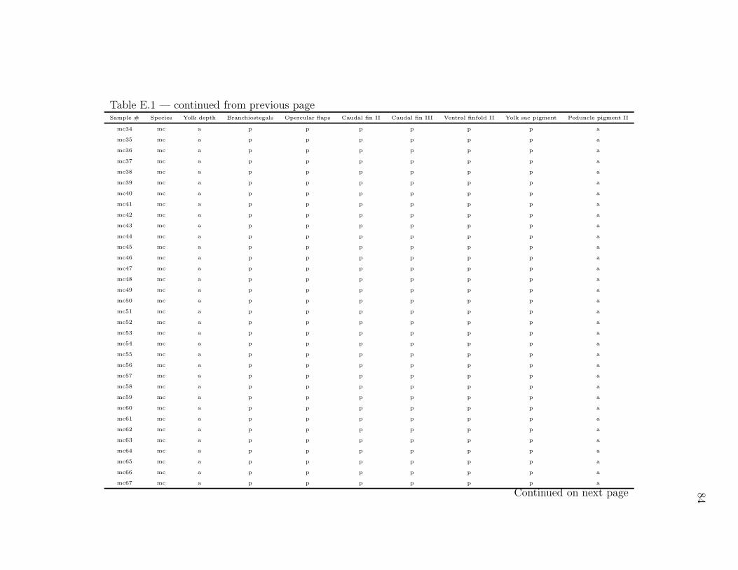
84
Table E.1 — continued from previous pageSample # Species Yolk depth Branchiostegals Opercular flaps Caudal fin II Caudal fin III Ventral finfold II Yolk sac pigment Peduncle pigment II
mc34 mc a p p p p p p a
mc35 mc a p p p p p p a
mc36 mc a p p p p p p a
mc37 mc a p p p p p p a
mc38 mc a p p p p p p a
mc39 mc a p p p p p p a
mc40 mc a p p p p p p a
mc41 mc a p p p p p p a
mc42 mc a p p p p p p a
mc43 mc a p p p p p p a
mc44 mc a p p p p p p a
mc45 mc a p p p p p p a
mc46 mc a p p p p p p a
mc47 mc a p p p p p p a
mc48 mc a p p p p p p a
mc49 mc a p p p p p p a
mc50 mc a p p p p p p a
mc51 mc a p p p p p p a
mc52 mc a p p p p p p a
mc53 mc a p p p p p p a
mc54 mc a p p p p p p a
mc55 mc a p p p p p p a
mc56 mc a p p p p p p a
mc57 mc a p p p p p p a
mc58 mc a p p p p p p a
mc59 mc a p p p p p p a
mc60 mc a p p p p p p a
mc61 mc a p p p p p p a
mc62 mc a p p p p p p a
mc63 mc a p p p p p p a
mc64 mc a p p p p p p a
mc65 mc a p p p p p p a
mc66 mc a p p p p p p a
mc67 mc a p p p p p p a
Continued on next page

85
Table E.1 — continued from previous pageSample # Species Yolk depth Branchiostegals Opercular flaps Caudal fin II Caudal fin III Ventral finfold II Yolk sac pigment Peduncle pigment II
mc68 mc a p p p p p p a
mr1 mr a a a a a a a a
mr2 mr a a a a a a a a
mr3 mr a a a a a a a a
mr4 mr a a a a a a a a
mr5 mr a a a a a a a a
mr6 mr a a a a a a a a
mr7 mr a a a a a a a a
mr8 mr a a a a a a a a
mr9 mr a a a a a a a a
mr10 mr a a a a a a a a
mr11 mr a a a a a a a a
mr12 mr a a a a a a a a
mr13 mr a a a a a a a a
mr14 mr a a a a a a a a
mr15 mr a a a a a a a a
mr16 mr a a a a a a a a
mr17 mr a a a a a a a a
mr18 mr a a a a a a a a
mr19 mr a a a a a a a a
mr20 mr a a a a a a a a
mr21 mr a a a a a a a a
mr22 mr a a a a a a a a
mr23 mr a a p p p p a a
mr24 mr a p p a a a a a
mr25 mr a p p p p p p a
mr26 mr a a a a p a p a
mr27 mr a p a p p p p a
mr28 mr a p p p a p a a
mr29 mr a a p p p a a a
mr30 mr a p p p a p p a
mr31 mr a p p p a a a a
mr32 mr a a p p p p p a
mr33 mr a p p p p p a a
Continued on next page

86
Table E.1 — continued from previous pageSample # Species Yolk depth Branchiostegals Opercular flaps Caudal fin II Caudal fin III Ventral finfold II Yolk sac pigment Peduncle pigment II
mr34 mr a p p p p p p a
mr35 mr a p p p p p p a
mr36 mr a p p p p p a a
mr37 mr a p p p p p p a
mr38 mr a p p p p p a a
mr39 mr a p p p p p a a
mr40 mr a p p p p p p a
mr41 mr a p p p p p p a
mr42 mr a p p p p p a a
mr43 mr a p p p p p p a
mr44 mr a p p p p p p a
mr45 mr a p p p p p p a
mr46 mr a p p p p p p a
mr47 mr a p p p p p p a
mr48 mr a p p p p p p a
mr49 mr a p p p p p p a
mr50 mr a p p p p p p a
mr51 mr a p p p p p p a
mr52 mr a p p p p p p a
mr53 mr a p p p p p p a
mr54 mr a p p p p p p a
mr55 mr a p p p p p p a
mr56 mr a p p p p p p a
mr57 mr a p p p p p p a
mr58 mr a p p p p p p a
mr59 mr a p p p p p p a
mr60 mr a p p p p p p a
mr61 mr a p p p p p p a
mr62 mr a p p p p p p a
mr63 mr a p p p p p p a
mr64 mr a p p p p p p a
mr65 mr a p p p p p p a
mr66 mr a p p p p p p a
mr67 mr a p p p p p p a
Continued on next page

87
Table E.1 — continued from previous pageSample # Species Yolk depth Branchiostegals Opercular flaps Caudal fin II Caudal fin III Ventral finfold II Yolk sac pigment Peduncle pigment II
mr68 mr a p p p p p p a
mr69 mr a p p p p p p a
mr70 mr a p p p p p p a
mr71 mr a p p p p p p a
mr72 mr a p p p p p p a
mr73 mr a p p p p p p a
mr74 mr a p p p p p p a
mr75 mr a p p p p p p a
mr76 mr a p p p p p p a
mr77 mr a p p p p p p a
mr78 mr a p p p p p p a
mr79 mr a p p p p p p a
mr80 mr a p p p p p p a
mr81 mr a p p p p p p a
Continued on next page

88
Table E.1 — continued from previous pageSample # Species Yolk depth II Nares Digestive tract Caudal fin IV Urostyle Dorsal fin Ventral finfold III Dorsum pigment
mc1 mc a a a u u a a a
mc2 mc a a a u u a a a
mc3 mc a a a u u a a a
mc4 mc a a a u u a a a
mc5 mc a a a u u a a a
mc6 mc a a a u u a a a
mc7 mc a a a u u a a a
mc8 mc a a a u u a a a
mc9 mc a a a u u a a a
mc10 mc a a a u u a a a
mc11 mc a a a u u a a a
mc12 mc a a a u u a a a
mc13 mc a a a a a a a a
mc14 mc a a a a a a a p
mc15 mc a a a a a p a a
mc16 mc a a a a a a a a
mc17 mc a a a a a a a a
mc18 mc a a a a a a a p
mc19 mc a a a p a a a p
mc20 mc a a a p a a p a
mc21 mc a a a a a a a a
mc22 mc a a a p a a a p
mc23 mc a a a p a a a p
mc24 mc a a a p a a a p
mc25 mc a a a p a a a a
mc26 mc a a a p a a a a
mc27 mc p p p p p p p a
mc28 mc p p p p p p p a
mc29 mc p p p p p p p p
mc30 mc p p p p p p p p
mc31 mc p p p p p p p p
mc32 mc p p p p p p p p
mc33 mc p p p p p p p p
Continued on next page
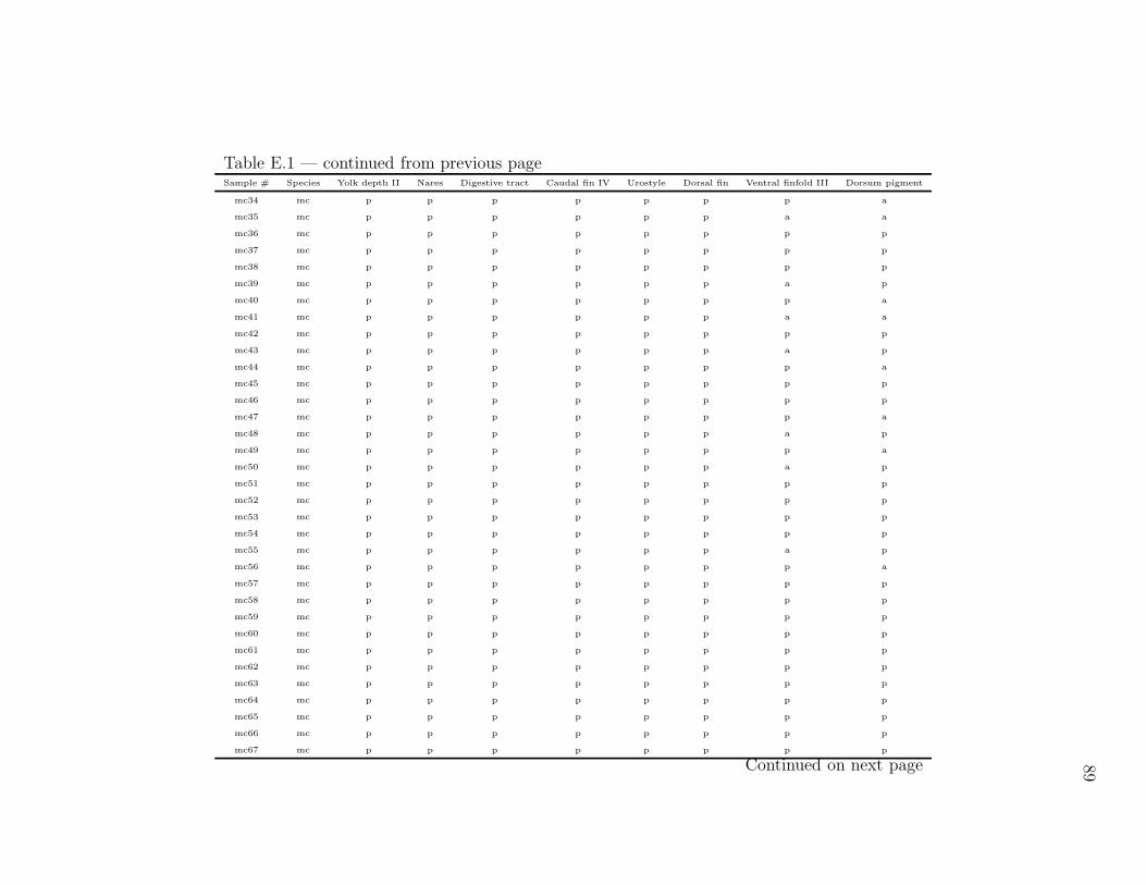
89
Table E.1 — continued from previous pageSample # Species Yolk depth II Nares Digestive tract Caudal fin IV Urostyle Dorsal fin Ventral finfold III Dorsum pigment
mc34 mc p p p p p p p a
mc35 mc p p p p p p a a
mc36 mc p p p p p p p p
mc37 mc p p p p p p p p
mc38 mc p p p p p p p p
mc39 mc p p p p p p a p
mc40 mc p p p p p p p a
mc41 mc p p p p p p a a
mc42 mc p p p p p p p p
mc43 mc p p p p p p a p
mc44 mc p p p p p p p a
mc45 mc p p p p p p p p
mc46 mc p p p p p p p p
mc47 mc p p p p p p p a
mc48 mc p p p p p p a p
mc49 mc p p p p p p p a
mc50 mc p p p p p p a p
mc51 mc p p p p p p p p
mc52 mc p p p p p p p p
mc53 mc p p p p p p p p
mc54 mc p p p p p p p p
mc55 mc p p p p p p a p
mc56 mc p p p p p p p a
mc57 mc p p p p p p p p
mc58 mc p p p p p p p p
mc59 mc p p p p p p p p
mc60 mc p p p p p p p p
mc61 mc p p p p p p p p
mc62 mc p p p p p p p p
mc63 mc p p p p p p p p
mc64 mc p p p p p p p p
mc65 mc p p p p p p p p
mc66 mc p p p p p p p p
mc67 mc p p p p p p p p
Continued on next page

90
Table E.1 — continued from previous pageSample # Species Yolk depth II Nares Digestive tract Caudal fin IV Urostyle Dorsal fin Ventral finfold III Dorsum pigment
mc68 mc p p p p p p p p
mr1 mr a a a u u a a a
mr2 mr a a a u u a a a
mr3 mr a a a u u a a a
mr4 mr a a a u u a a a
mr5 mr a a a u u a a a
mr6 mr a a a u u a a a
mr7 mr a a a u u a a a
mr8 mr a a a u u a a a
mr9 mr a a a u u a a a
mr10 mr a a a u u a a a
mr11 mr a a a u u a a a
mr12 mr a a a u u a a a
mr13 mr a a a u u a a a
mr14 mr a a a u u a a a
mr15 mr a a a u u a a a
mr16 mr a a a u u a a a
mr17 mr a a a u u a a a
mr18 mr a a a u u a a a
mr19 mr a a a u u a a a
mr20 mr a a a u u a a a
mr21 mr a a a u u a a a
mr22 mr a a a u u a a a
mr23 mr a a a u u a a a
mr24 mr a a a u u a a a
mr25 mr a a a u u a a a
mr26 mr a a a u u a a a
mr27 mr a a a u u a a a
mr28 mr a a a u u a a a
mr29 mr a a a u u a a a
mr30 mr a a a u u a a a
mr31 mr a a a u u a a a
mr32 mr a a a u u a a a
mr33 mr a a a u u a a a
Continued on next page

91
Table E.1 — continued from previous pageSample # Species Yolk depth II Nares Digestive tract Caudal fin IV Urostyle Dorsal fin Ventral finfold III Dorsum pigment
mr34 mr p p a p p p a p
mr35 mr p p p p p p p a
mr36 mr a p a p p p a p
mr37 mr a p a p p a p p
mr38 mr p p a p p p p p
mr39 mr a p a p p p p p
mr40 mr a p a p p p p p
mr41 mr p p p p p p p a
mr42 mr p p p p p p p p
mr43 mr p p a p p p p p
mr44 mr p p p p p p p p
mr45 mr p p p p p p p a
mr46 mr p p p p p p p p
mr47 mr p p p p p p p p
mr48 mr p p p p p p p p
mr49 mr p p p p p p a p
mr50 mr p p p p p p p p
mr51 mr p p p p p p p p
mr52 mr p p p p p p a p
mr53 mr p p p p p p p p
mr54 mr p p p p p p a p
mr55 mr p p p p p p p p
mr56 mr p p p p p p p p
mr57 mr p p p p p p p p
mr58 mr p p p p p p p p
mr59 mr p p p p p p p p
mr60 mr p p p p p p p p
mr61 mr p p p p p p p p
mr62 mr p p p p p p p p
mr63 mr p p p p p p p p
mr64 mr p p p p p p p p
mr65 mr p p p p p p p p
mr66 mr p p p p p p a p
mr67 mr p p p p p p p p
Continued on next page
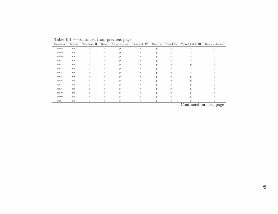
92
Table E.1 — continued from previous pageSample # Species Yolk depth II Nares Digestive tract Caudal fin IV Urostyle Dorsal fin Ventral finfold III Dorsum pigment
mr68 mr p p p p p p a p
mr69 mr p p p p p p a p
mr70 mr p p p p p p a p
mr71 mr p p p p p p a p
mr72 mr p p p p p p p p
mr73 mr p p p p p p a p
mr74 mr p p p p p p a p
mr75 mr p p p p p p p p
mr76 mr p p p p p p p p
mr77 mr p p p p p p p p
mr78 mr p p p p p p p p
mr79 mr p p p p p p p p
mr80 mr p p p p p p p p
mr81 mr p p p p p p p p
Continued on next page

93
Table E.1 — continued from previous pageSample # Species Chin pigment Yolk sac Mouth position Pelvic fins Dorsal fin margins Dorsal finfold Anal fin Arrow-shaped pigment
mc1 mc p a u a u u a a
mc2 mc p a u a u u a a
mc3 mc p a u a u u a a
mc4 mc p a u a u u a a
mc5 mc p a u a u u a a
mc6 mc p a u a u u a a
mc7 mc p a u a u u a a
mc8 mc p a u a u u a a
mc9 mc p a u a u u a a
mc10 mc p a u a u u a a
mc11 mc p a u a u u a a
mc12 mc p a u a u u a a
mc13 mc p a u a u u a a
mc14 mc p a u a u u a a
mc15 mc p a u a u u a a
mc16 mc p a u a u u a a
mc17 mc p a u a u u a a
mc18 mc p a u a u u a a
mc19 mc p a u a u u a a
mc20 mc p a u a u u a a
mc21 mc p a u a u u a a
mc22 mc p a u a u u a a
mc23 mc p a u a u u a a
mc24 mc p a u a u u a a
mc25 mc p a u a u u a a
mc26 mc p a u a u u a a
mc27 mc p a a a a a p a
mc28 mc p a a a a a a p
mc29 mc p a a a a a p p
mc30 mc p a a a a a p p
mc31 mc p a a a a a p p
mc32 mc p a a a a a p p
mc33 mc p a a a a a p p
Continued on next page

94
Table E.1 — continued from previous pageSample # Species Chin pigment Yolk sac Mouth position Pelvic fins Dorsal fin margins Dorsal finfold Anal fin Arrow-shaped pigment
mc34 mc p a a a a a p p
mc35 mc p a a a a a a p
mc36 mc p a a a a a p p
mc37 mc p a a a a a p p
mc38 mc p a a a a a p p
mc39 mc p a a a a a p p
mc40 mc p a a a a a p p
mc41 mc p a a a a a a p
mc42 mc p a a a a a p p
mc43 mc p a a a a a p p
mc44 mc p a a a a a p p
mc45 mc p p a a a a p p
mc46 mc p a a a a a p p
mc47 mc p a a a a a p p
mc48 mc p a a a a a p p
mc49 mc p a a a a a p a
mc50 mc p a a a a a p p
mc51 mc a p a a a a p p
mc52 mc p p a a a a p p
mc53 mc p a a a a a p p
mc54 mc a p a a a a p p
mc55 mc p p a a a a p p
mc56 mc p a a a a a p p
mc57 mc p a a a a a p p
mc58 mc a p a a a a p p
mc59 mc p a a a a a p p
mc60 mc a p p p p p p p
mc61 mc a p p p p p p p
mc62 mc a p p p p p p p
mc63 mc a p p p p p p p
mc64 mc a p p p p p p p
mc65 mc a p p p p p p p
mc66 mc a p p p p p p p
mc67 mc a p p p p p p p
Continued on next page

95
Table E.1 — continued from previous pageSample # Species Chin pigment Yolk sac Mouth position Pelvic fins Dorsal fin margins Dorsal finfold Anal fin Arrow-shaped pigment
mc68 mc a p p p p p p p
mr1 mr p a u a u u a a
mr2 mr p a u a u u a a
mr3 mr p a u a u u a a
mr4 mr p a u a u u a a
mr5 mr p a u a u u a a
mr6 mr p a u a u u a a
mr7 mr p a u a u u a a
mr8 mr p a u a u u a a
mr9 mr p a u a u u a a
mr10 mr p a u a u u a a
mr11 mr p a u a u u a a
mr12 mr p a u a u u a a
mr13 mr p a u a u u a a
mr14 mr p a u a u u a a
mr15 mr p a u a u u a a
mr16 mr p a u a u u a a
mr17 mr p a u a u u a a
mr18 mr p a u a u u a a
mr19 mr p a u a u u a a
mr20 mr p a u a u u a a
mr21 mr p a u a u u a a
mr22 mr p a u a u u a a
mr23 mr p a u a u u a a
mr24 mr p a u a u u a a
mr25 mr p a u a u u a a
mr26 mr p a u a u u a a
mr27 mr p a u a u u a a
mr28 mr p a u a u u a a
mr29 mr p a u a u u a a
mr30 mr p a u a u u a a
mr31 mr p a u a u u a a
mr32 mr p a u a u u a a
mr33 mr p a u a u u a a
Continued on next page

96
Table E.1 — continued from previous pageSample # Species Chin pigment Yolk sac Mouth position Pelvic fins Dorsal fin margins Dorsal finfold Anal fin Arrow-shaped pigment
mr34 mr p a u a u u a a
mr35 mr p a u a u u a a
mr36 mr p a u a u u a a
mr37 mr p a u a u u a a
mr38 mr p a u a u u a a
mr39 mr p a u a u u a a
mr40 mr p a u a u u a a
mr41 mr p a u a u u a a
mr42 mr p a u a u u a a
mr43 mr p a u a u u a a
mr44 mr a p a p p p p p
mr45 mr a p p p p p a p
mr46 mr a a a p p p a a
mr47 mr a a a p p p a a
mr48 mr a p a p p p a a
mr49 mr a a p p p p p p
mr50 mr a p p p p p p p
mr51 mr a a a p p p a a
mr52 mr a p p p p p p p
mr53 mr a p p p p p p p
mr54 mr a p p p p p a p
mr55 mr a p p p p p a p
mr56 mr a p p p p p p p
mr57 mr a p p p p p p p
mr58 mr a p p p p p p p
mr59 mr a p p p p p a p
mr60 mr a p p p p p p p
mr61 mr a p p p p p p p
mr62 mr a p p p p p a p
mr63 mr a p p p p p p p
mr64 mr a p p p p p p p
mr65 mr a p p p p p p p
mr66 mr a p p p p p p p
mr67 mr a p p p p p p p
Continued on next page

97
Table E.1 — continued from previous pageSample # Species Chin pigment Yolk sac Mouth position Pelvic fins Dorsal fin margins Dorsal finfold Anal fin Arrow-shaped pigment
mr68 mr a p p p p p p p
mr69 mr a p p p p p p p
mr70 mr a p p p p p p p
mr71 mr a p p p p p p p
mr72 mr a p p p p p p p
mr73 mr a p p p p p p p
mr74 mr a p p p p p a p
mr75 mr a p p p p p a p
mr76 mr a p p p p p a p
mr77 mr a p p p p p a p
mr78 mr a p p p p p a p
mr79 mr a p p p p p a p
mr80 mr a p p p p p p p
mr81 mr a p p p p p a p
Continued on next page

98
Table E.1 — continued from previous pageSample # Species Gut melanophores Jaw pigment Gill arch pigment Mouth position II Anal fin II Pelvic flaps Dorsal finfold II Ventral finfold IV
mc1 mc a a a a a a u u
mc2 mc a a a a a a u u
mc3 mc a a a a a a u u
mc4 mc a a a a a a u u
mc5 mc a a a a a a u u
mc6 mc a a a a a a u u
mc7 mc a a a a a a u u
mc8 mc a a a a a a u u
mc9 mc a a a a a a u u
mc10 mc a a a a a a u u
mc11 mc a a a a a a u u
mc12 mc a a a a a a u u
mc13 mc a a a a a a u u
mc14 mc a a a a a a u u
mc15 mc a a a a a a u u
mc16 mc a a a a a a u u
mc17 mc a a a a a a u u
mc18 mc a a a a a a u u
mc19 mc a a a a a a u u
mc20 mc a a a a a a u u
mc21 mc a a a a a a u u
mc22 mc a a a a a a u u
mc23 mc a a a a a a u u
mc24 mc a a a a a a u u
mc25 mc a a a a a a u u
mc26 mc a a a a a a u u
mc27 mc a a a a a a a a
mc28 mc a a a a a a a a
mc29 mc a a a a a a a a
mc30 mc a a a a a a a a
mc31 mc a a a a a a a a
mc32 mc a a a a a a a a
mc33 mc a a a a a a a a
Continued on next page

99
Table E.1 — continued from previous pageSample # Species Gut melanophores Jaw pigment Gill arch pigment Mouth position II Anal fin II Pelvic flaps Dorsal finfold II Ventral finfold IV
mc34 mc a a a a a a a a
mc35 mc a a a a a a a a
mc36 mc a a a a a a a a
mc37 mc a a a a a a a a
mc38 mc a a a a a a a a
mc39 mc a a a a a a a a
mc40 mc a a a a a a a a
mc41 mc a a a a a a a a
mc42 mc a a a a a a a a
mc43 mc p a a a a a a a
mc44 mc a a a a a a a a
mc45 mc a a a a a a a a
mc46 mc a a a a a a a a
mc47 mc a a a a a a a a
mc48 mc a a a a a a a a
mc49 mc a a a a a a a a
mc50 mc p a a a a a a a
mc51 mc a a a a a a a a
mc52 mc a a a a a a a a
mc53 mc a a a a a a a a
mc54 mc a a a a a a a a
mc55 mc a a a a a a a a
mc56 mc a a a a a a a a
mc57 mc a a a a a a a a
mc58 mc a a a a a a a a
mc59 mc a a a a a a a a
mc60 mc a p a a a a a a
mc61 mc a p p a a a a a
mc62 mc a p p p p p p a
mc63 mc a p p p p p p a
mc64 mc a p p p p p p p
mc65 mc a p p p p p p p
mc66 mc a p p p p p p a
mc67 mc a p p p p p p a
Continued on next page

100
Table E.1 — continued from previous pageSample # Species Gut melanophores Jaw pigment Gill arch pigment Mouth position II Anal fin II Pelvic flaps Dorsal finfold II Ventral finfold IV
mc68 mc a p p p p p p a
mr1 mr a a a a a a u u
mr2 mr a a a a a a u u
mr3 mr a a a a a a u u
mr4 mr a a a a a a u u
mr5 mr a a a a a a u u
mr6 mr a a a a a a u u
mr7 mr a a a a a a u u
mr8 mr a a a a a a u u
mr9 mr a a a a a a u u
mr10 mr a a a a a a u u
mr11 mr a a a a a a u u
mr12 mr a a a a a a u u
mr13 mr a a a a a a u u
mr14 mr a a a a a a u u
mr15 mr a a a a a a u u
mr16 mr a a a a a a u u
mr17 mr a a a a a a u u
mr18 mr a a a a a a u u
mr19 mr a a a a a a u u
mr20 mr a a a a a a u u
mr21 mr a a a a a a u u
mr22 mr a a a a a a u u
mr23 mr a a a a a a u u
mr24 mr a a a a a a u u
mr25 mr a a a a a a u u
mr26 mr a a a a a a u u
mr27 mr a a a a a a u u
mr28 mr a a a a a a u u
mr29 mr a a a a a a u u
mr30 mr a a a a a a u u
mr31 mr a a a a a a u u
mr32 mr a a a a a a u u
mr33 mr a a a a a a u u
Continued on next page

101
Table E.1 — continued from previous pageSample # Species Gut melanophores Jaw pigment Gill arch pigment Mouth position II Anal fin II Pelvic flaps Dorsal finfold II Ventral finfold IV
mr34 mr a a a a a a u u
mr35 mr a a a a a a u u
mr36 mr a a a a a a u u
mr37 mr a a a a a a u u
mr38 mr a a a a a a u u
mr39 mr a a a a a a u u
mr40 mr a a a a a a u u
mr41 mr a a a a a a u u
mr42 mr a a a a a a u u
mr43 mr a a a a a a u u
mr44 mr a p a a a a a a
mr45 mr p p a a a a a a
mr46 mr a p a a a a a a
mr47 mr a p a a a a a a
mr48 mr a p a a a a a a
mr49 mr a p a a a a a a
mr50 mr a p a a a a a a
mr51 mr a p a a a a a a
mr52 mr a p a a a a a a
mr53 mr a p a a a a a a
mr54 mr a p p p p p p a
mr55 mr a p p p p p p a
mr56 mr a p p p p p p a
mr57 mr a p p p p p p a
mr58 mr a p p p p p p a
mr59 mr a p p p p p p a
mr60 mr a p p p p p p a
mr61 mr a p p p p p p a
mr62 mr a p p p p p p a
mr63 mr a p p p p p p a
mr64 mr a p p p p p p a
mr65 mr a p p p p p p p
mr66 mr a p p p p p p p
mr67 mr a p p p p p p a
Continued on next page

102
Table E.1 — continued from previous pageSample # Species Gut melanophores Jaw pigment Gill arch pigment Mouth position II Anal fin II Pelvic flaps Dorsal finfold II Ventral finfold IV
mr68 mr a p p p p p p p
mr69 mr a p p p p p p p
mr70 mr a p p p p p p p
mr71 mr a p p p p p p p
mr72 mr a p p p p p p p
mr73 mr a p p p p p p p
mr74 mr a p p p p p p p
mr75 mr a p p p p p p p
mr76 mr a p p p p p p p
mr77 mr a p p p p p p p
mr78 mr a p p p p p p p
mr79 mr a p p p p p p p
mr80 mr a p p p p p p p
mr81 mr a p p p p p p p
Continued on next page

103
Table E.1 — continued from previous pageSample # Species Operculum length Pelvic fins Lip pigment Snout pigment Jaw pigment II Head profile Dorsal fin profile Anal fin III
mc1 mc u u u u u a u u
mc2 mc u u u u u a u u
mc3 mc u u u u u a u u
mc4 mc u u u u u a u u
mc5 mc u u u u u a u u
mc6 mc u u u u u a u u
mc7 mc u u u u u a u u
mc8 mc u u u u u a u u
mc9 mc u u u u u a u u
mc10 mc u u u u u a u u
mc11 mc u u u u u a u u
mc12 mc u u u u u a u u
mc13 mc u u u u u a u u
mc14 mc u u u u u a u u
mc15 mc u u u u u a u u
mc16 mc u u u u u a u u
mc17 mc u u u u u a u u
mc18 mc u u u u u a u u
mc19 mc u u u u u a u u
mc20 mc u u u u u a u u
mc21 mc u u u u u a u u
mc22 mc u u u u u a u u
mc23 mc u u u u u a u u
mc24 mc u u u u u a u u
mc25 mc u u u u u a u u
mc26 mc u u u u u a u u
mc27 mc u u u u u a u u
mc28 mc u u u u u a u u
mc29 mc u u u u u a u u
mc30 mc u u u u u a u u
mc31 mc u u u u u a u u
mc32 mc u u u u u a u u
mc33 mc u u u u u a u u
Continued on next page

104
Table E.1 — continued from previous pageSample # Species Operculum length Pelvic fins Lip pigment Snout pigment Jaw pigment II Head profile Dorsal fin profile Anal fin III
mc34 mc u u u u u a u u
mc35 mc u u u u u a u u
mc36 mc u u u u u a u u
mc37 mc u u u u u a u u
mc38 mc u u u u u a u u
mc39 mc u u u u u a u u
mc40 mc u u u u u a u u
mc41 mc u u u u u a u u
mc42 mc u u u u u a u u
mc43 mc u u u u u a u u
mc44 mc u u u u u a u u
mc45 mc u u u u u a u u
mc46 mc u u u u u a u u
mc47 mc u u u u u a u u
mc48 mc u u u u u a u u
mc49 mc u u u u u a u u
mc50 mc u u u u u a u u
mc51 mc u u u u u a u u
mc52 mc u u u u u a u u
mc53 mc u u u u u a u u
mc54 mc u u u u u a u u
mc55 mc u u u u u a u u
mc56 mc u u u u u a u u
mc57 mc u u u u u a u u
mc58 mc u u u u u a u u
mc59 mc u u u u u a u u
mc60 mc u u u u u a u u
mc61 mc u u u u u a u u
mc62 mc a p a a u a u u
mc63 mc a p a a u a u u
mc64 mc a p a a u a u u
mc65 mc p p a a a a a a
mc66 mc p p a a a a a a
mc67 mc p p a a p a a p
Continued on next page

105
Table E.1 — continued from previous pageSample # Species Operculum length Pelvic fins Lip pigment Snout pigment Jaw pigment II Head profile Dorsal fin profile Anal fin III
mc68 mc p p a a p a a p
mr1 mr u u u u u a u u
mr2 mr u u u u u a u u
mr3 mr u u u u u a u u
mr4 mr u u u u u a u u
mr5 mr u u u u u a u u
mr6 mr u u u u u a u u
mr7 mr u u u u u a u u
mr8 mr u u u u u a u u
mr9 mr u u u u u a u u
mr10 mr u u u u u a u u
mr11 mr u u u u u a u u
mr12 mr u u u u u a u u
mr13 mr u u u u u a u u
mr14 mr u u u u u a u u
mr15 mr u u u u u a u u
mr16 mr u u u u u a u u
mr17 mr u u u u u a u u
mr18 mr u u u u u a u u
mr19 mr u u u u u a u u
mr20 mr u u u u u a u u
mr21 mr u u u u u a u u
mr22 mr u u u u u a u u
mr23 mr u u u u u a u u
mr24 mr u u u u u a u u
mr25 mr u u u u u a u u
mr26 mr u u u u u a u u
mr27 mr u u u u u a u u
mr28 mr u u u u u a u u
mr29 mr u u u u u a u u
mr30 mr u u u u u a u u
mr31 mr u u u u u a u u
mr32 mr u u u u u a u u
mr33 mr u u u u u a u u
Continued on next page

106
Table E.1 — continued from previous pageSample # Species Operculum length Pelvic fins Lip pigment Snout pigment Jaw pigment II Head profile Dorsal fin profile Anal fin III
mr34 mr u u u u u a u u
mr35 mr u u u u u a u u
mr36 mr u u u u u a u u
mr37 mr u u u u u a u u
mr38 mr u u u u u a u u
mr39 mr u u u u u a u u
mr40 mr u u u u u a u u
mr41 mr u u u u u a u u
mr42 mr u u u u u a u u
mr43 mr u u u u u a u u
mr44 mr u u u u u a u u
mr45 mr u u u u u a u u
mr46 mr u u u u u a u u
mr47 mr u u u u u a u u
mr48 mr u u u u u a u u
mr49 mr u u u u u a u u
mr50 mr u u u u u a u u
mr51 mr u u u u u a u u
mr52 mr u u u u u a u u
mr53 mr u u u u u a u u
mr54 mr u a u u u a u u
mr55 mr u a u u u a u u
mr56 mr u a u u u a u u
mr57 mr u a u u u a u u
mr58 mr u a u u u a u u
mr59 mr u a u u u a u u
mr60 mr u a u u u a u u
mr61 mr u a u u u a u u
mr62 mr u a u u u a u u
mr63 mr u a u u u a u u
mr64 mr p p a a u a u u
mr65 mr p p a a u a u u
mr66 mr p p a a u a u u
mr67 mr a p a a u a u u
Continued on next page
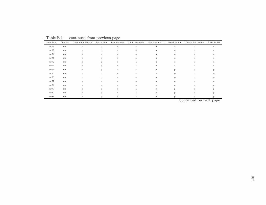
107
Table E.1 — continued from previous pageSample # Species Operculum length Pelvic fins Lip pigment Snout pigment Jaw pigment II Head profile Dorsal fin profile Anal fin III
mr68 mr p p a a u a u u
mr69 mr p p a a u a u u
mr70 mr p p a a u a u u
mr71 mr p p a a u a u u
mr72 mr p p a a u a u u
mr73 mr p p a a u a u u
mr74 mr p p a a p p p p
mr75 mr p p a a a p p p
mr76 mr p p a a p p p p
mr77 mr p p a a p p p p
mr78 mr p p a a p p p p
mr79 mr p p a a p p p p
mr80 mr p p a a p p p p
mr81 mr p p a a p p p p
Continued on next page
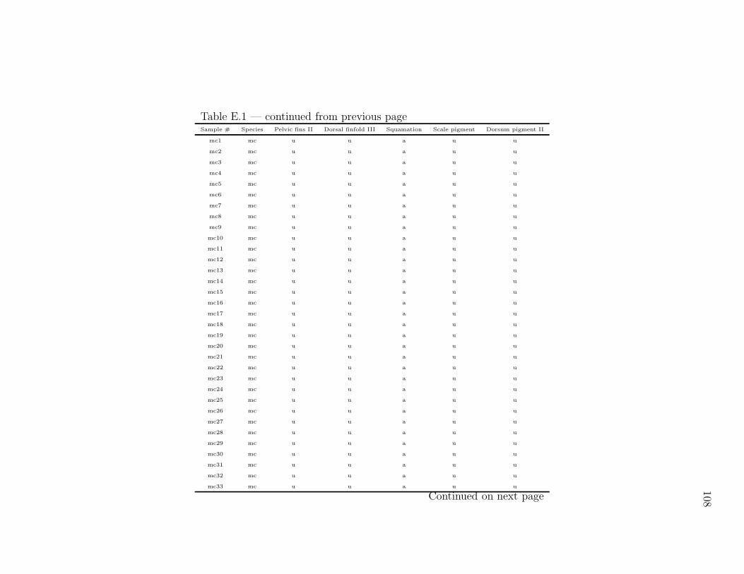
108
Table E.1 — continued from previous pageSample # Species Pelvic fins II Dorsal finfold III Squamation Scale pigment Dorsum pigment II
mc1 mc u u a u u
mc2 mc u u a u u
mc3 mc u u a u u
mc4 mc u u a u u
mc5 mc u u a u u
mc6 mc u u a u u
mc7 mc u u a u u
mc8 mc u u a u u
mc9 mc u u a u u
mc10 mc u u a u u
mc11 mc u u a u u
mc12 mc u u a u u
mc13 mc u u a u u
mc14 mc u u a u u
mc15 mc u u a u u
mc16 mc u u a u u
mc17 mc u u a u u
mc18 mc u u a u u
mc19 mc u u a u u
mc20 mc u u a u u
mc21 mc u u a u u
mc22 mc u u a u u
mc23 mc u u a u u
mc24 mc u u a u u
mc25 mc u u a u u
mc26 mc u u a u u
mc27 mc u u a u u
mc28 mc u u a u u
mc29 mc u u a u u
mc30 mc u u a u u
mc31 mc u u a u u
mc32 mc u u a u u
mc33 mc u u a u u
Continued on next page

109
Table E.1 — continued from previous pageSample # Species Pelvic fins II Dorsal finfold III Squamation Scale pigment Dorsum pigment II
mc34 mc u u a u u
mc35 mc u u a u u
mc36 mc u u a u u
mc37 mc u u a u u
mc38 mc u u a u u
mc39 mc u u a u u
mc40 mc u u a u u
mc41 mc u u a u u
mc42 mc u u a u u
mc43 mc u u a u u
mc44 mc u u a u u
mc45 mc u u a u u
mc46 mc u u a u u
mc47 mc u u a u u
mc48 mc u u a u u
mc49 mc u u a u u
mc50 mc u u a u u
mc51 mc u u a u u
mc52 mc u u a u u
mc53 mc u u a u u
mc54 mc u u a u u
mc55 mc u u a u u
mc56 mc u u a u u
mc57 mc u u a u u
mc58 mc u u a u u
mc59 mc u u a u u
mc60 mc u u a u u
mc61 mc u u a u u
mc62 mc u u a u u
mc63 mc u u a u u
mc64 mc u u a u u
mc65 mc a p a u u
mc66 mc p a a u u
mc67 mc a p a p p
Continued on next page

110
Table E.1 — continued from previous pageSample # Species Pelvic fins II Dorsal finfold III Squamation Scale pigment Dorsum pigment II
mc68 mc p a a a p
mr1 mr u u a a u
mr2 mr u u a a u
mr3 mr u u a a u
mr4 mr u u a a u
mr5 mr u u a a u
mr6 mr u u a a u
mr7 mr u u a a u
mr8 mr u u a a u
mr9 mr u u a a u
mr10 mr u u a a u
mr11 mr u u a a u
mr12 mr u u a a u
mr13 mr u u a a u
mr14 mr u u a a u
mr15 mr u u a a u
mr16 mr u u a a u
mr17 mr u u a a u
mr18 mr u u a a u
mr19 mr u u a a u
mr20 mr u u a a u
mr21 mr u u a a u
mr22 mr u u a a u
mr23 mr u u a a u
mr24 mr u u a a u
mr25 mr u u a a u
mr26 mr u u a a u
mr27 mr u u a a u
mr28 mr u u a a u
mr29 mr u u a a u
mr30 mr u u a a u
mr31 mr u u a a u
mr32 mr u u a a u
mr33 mr u u a a u
Continued on next page

111
Table E.1 — continued from previous pageSample # Species Pelvic fins II Dorsal finfold III Squamation Scale pigment Dorsum pigment II
mr34 mr u u a a u
mr35 mr u u a a u
mr36 mr u u a a u
mr37 mr u u a a u
mr38 mr u u a a u
mr39 mr u u a a u
mr40 mr u u a a u
mr41 mr u u a a u
mr42 mr u u a a u
mr43 mr u u a a u
mr44 mr u u a a u
mr45 mr u u a a u
mr46 mr u u a a u
mr47 mr u u a a u
mr48 mr u u a a u
mr49 mr u u a a u
mr50 mr u u a a u
mr51 mr u u a a u
mr52 mr u u a a u
mr53 mr u u a a u
mr54 mr u u a a u
mr55 mr u u a a u
mr56 mr u u a a u
mr57 mr u u a a u
mr58 mr u u a a u
mr59 mr u u a a u
mr60 mr u u a a u
mr61 mr u u a a u
mr62 mr u u a a u
mr63 mr u u a a u
mr64 mr u u a a u
mr65 mr u u a a u
mr66 mr u u a a u
mr67 mr u u a a u
Continued on next page

112
Table E.1 — continued from previous pageSample # Species Pelvic fins II Dorsal finfold III Squamation Scale pigment Dorsum pigment II
mr68 mr u u a a u
mr69 mr u u a a u
mr70 mr u u a a u
mr71 mr u u a a u
mr72 mr u u a a u
mr73 mr u u a a u
mr74 mr p p a a u
mr75 mr p p a a u
mr76 mr p p a a u
mr77 mr p p a a u
mr78 mr p p a a u
mr79 mr p p a a u
mr80 mr p p p p p
mr81 mr p p p p p
Continued on next page
Recommended