1
Universidade de Aveiro 2009
Departamento de Electrónica, Telecomunicações e Informática
Rui Manuel Fernandes Inácio
VoIP Service Performance Evaluation over 3GPP networks Avaliação de Desempenho do funcionamento de serviços VoIP sobre redes 3GPP

2
Universidade de Aveiro 2008
Departamento de Electrónica, Telecomunicações e Informática
Rui Manuel Fernandes Inácio
VoIP Service Performance Evaluation over 3GPP networks Avaliação de Desempenho do funcionamento de serviços VoIP sobre redes 3GPP
Dissertação apresentada à Universidade de Aveiro para cumprimento dos requisitos necessários à obtenção do grau de Mestre em Engenharia Electrónica e de Telecomunicações (Mestrado Integrado), realizada sob a orientação científica da Professora Dra. Susana Sargento, Professora auxiliar do Departamento de Electrónica, Telecomunicações e Informática da Universidade de Aveiro e do Mestre Miguel Almeida, Engenheiro da Nokia Siemens Networks.

3
o júri
presidente
Prof. Doutor Atílio Gameiro
Professor associado do Departamento de Electrónica, Telecomunicações e Informática da Universidade de Aveiro
orientador
Prof. Doutora Susana Isabel Barreto de Miranda Sargento
Professora auxiliar do Departamento de Electrónica, Telecomunicações e Informática da Universidade de Aveiro
Arguente
Prof. Doutor Jorge Sá Silva
Professor auxiliar do Departamento de Engenharia Informática da Faculdade de Ciências e Tecnologia da Universidade de Coimbra

4
agradecimentos
Este trabalho é o culminar de um importante processo de investimento pessoal e profissional, na contínua formação enquanto homem, pessoa e profissional. De realçar que o desenvolvimento deste trabalho não teria sido possível sem o contributo directo e indirecto, de todas as pessoas que trabalharam comigo no último ano e meio e às quais deixo o mais sincero agradecimento. Uma palavra de agradecimento para a minha orientadora Prof. Dra. Susana Sargento pela disponibilidade e orientação ao longo deste trabalho. O meu agradecimento profundo ao Miguel Almeida pela troca de ideias, orientação, motivação, entre-ajuda nos projectos comuns e companheirismo, sem o qual este trabalho teria sido muito mais complicado de definir. Ao meu colaborador Lucas Guarbalden, pela disponibilidade, força e tenacidade demonstrada no apoio prestado, um grande obrigado. Por último mas não menos importante um agradecimento profundo à paciência, confiança e fé depositadas no meu trabalho pela minha esposa Maria. A tua força e dedicação a nós foram fundamentais para o sucesso do meu trabalho. À minha Alice pela sua companhia e amor incondicional deixo uma palavra de agradecimento.

5
palavras-chave
UMTS, HSPA, HSDPA, HSUPA, VoIP, Performance, Monitoring, OSS, Reporting, KPI
resumo
A gestão de conteúdos orientados ao utilizador tem-se vindo a revelar uma questão de extrema importância para os operadores, que embora não sejam os produtores e distribuidores da informação acedida, são no entanto parte interessada pois em última análise é a sua insignia que deve assegurar o acesso. Os modelos de negócio desenvolvidos actualmente antevêm a distribuição destes conteúdos assegurando o cumprimento dos parâmetros de QoS. Com a evolução da distribuição de serviços sobre as redes IP, seguindo a tendência da perspectiva “All-over-IP”, os ISPs necessitam cada vez mais de ter conhecimento acerca da forma como estes serviços e os seus utilizadores influenciam a utilização dos recursos da rede. A monitorização de desempenho requer estratégias eficientes e optimizadas com múltiplas implicações ao nível da segurança/privacidade. Cada serviçopossui características específicas que o podem tornar mais ou menos resistente a determinadas condições da rede. O objectivo deste trabalho é relacionar a informação relativa à sessão de um determinado tipo de serviçobaseado em IP, com as condições de desempenho na entrega do serviço por parte da rede. O desafio é analisar diferentes tipos de informação, por um lado a informação de sessão foca-se nos eventos gerados durante o seu ciclo de vida, enquanto a informação de Performance Management (PM) da rede foca-se primordialmente no comportamento e capacidade da rede em suportar a entrega do serviço, a um grande número de assinantes, relevando portanto a utilização das métricas de QoS. A proposta deste trabalho é definir uma série de ferramentas como relatórios e indicadores de desempenho, em que baseado na informação cross-layer, se possa descrever uniformemente o desempenho do serviço.

6
keywords
UMTS, HSPA, HSDPA, HSUPA, VoIP, Performance, Monitoring, OSS, Reporting, KPI
abstract
The management of user oriented contents is becoming of extreme relevance for network operators, which while not being the producers of the consumed data, are the ultimate insignia for the assured delivery. The business models being currently applied envision the assured delivery of multimedia services with the assurance of Quality of Service. By evolving towards the delivery of services over IP networks undergoing the “all-over-IP” perspective, the Internet Service Providers (ISP) needs to be aware of how the behavior of these services and users influences the network resources usage. Performance monitoring requires efficient and optimized strategies with multiple implications at the security/privacy levels. Each service has specific characteristics which may make it more or less resilient to some network performance issues. The scope of this work is to relate session information with the underlying network service delivery performance. The challenge is to analyze different kind of information, session information focus is event driven tracing the entire life-cycle of each event and network Performance Management (PM) informationfocusing on the behavior and ability of the network to support service delivery to a large number of subscribers, thus focusing on overall QoS metrics. The proposal is to define use cases that can be implemented to ease this analysis while defining general Key Performance Indicators (KPI) based on cross-layer information, to uniformly describe the service performance.
7
Table of ContentsTable of ContentsTable of ContentsTable of Contents
Table of Contents......................................................................................................... 7 Index of Figures ........................................................................................................... 9 Index of Tables........................................................................................................... 11 Acronyms................................................................................................................... 12 1. Introduction ....................................................................................................... 17
1.1. Motivation .................................................................................................. 18 1.2. Objectives ................................................................................................... 20 1.3. Contributions of the Thesis ........................................................................ 22 1.4. Organization of the Thesis ......................................................................... 23
2. Background ........................................................................................................ 24 2.1. Network Management................................................................................ 24
2.1.1. TMN Logical Model............................................................................ 25 2.1.2. Performance Management Techniques .............................................. 27
2.2. Packet Switched Networks......................................................................... 28 2.2.1. Network Architecture ........................................................................ 28 2.2.2. Packet Session Establishment Procedure............................................ 31
2.3. High-Speed Packet Access.......................................................................... 36 2.3.1. UMTS R99 before HSPA..................................................................... 36 2.3.2. High-Speed Downlink Packet Access (HSDPA)................................. 37 2.3.3. High-Speed Uplink Packet Access (HSUPA)...................................... 41
2.4. LTE/SAE Evolution .................................................................................... 47 2.5. Summary .................................................................................................... 51
3. Performance Management ................................................................................. 52 3.1. Architecture Overview .............................................................................. 52 3.2. Metadata ..................................................................................................... 55
3.2.1. Configuration Management (CM) ...................................................... 55 3.2.2. Performance Management (PM) ........................................................ 56 3.2.3. Fault Management (FM) ..................................................................... 56
3.3. Data Sources ............................................................................................... 57 3.4. Extraction, Transformation and Loading Process ...................................... 67 3.5. Object Model .............................................................................................. 68 3.6. Key Performance Indicators....................................................................... 71
3.6.1. Network Session – Control Plane KPIs............................................... 72 3.6.2. Network Session – User Plane KPIs.................................................... 80 3.6.3. Service Session – Service Performance Indicators.............................. 88
3.7. Reports........................................................................................................ 91 3.8. Conclusion................................................................................................ 100
4. Simulation ........................................................................................................ 102 4.1. Simulation Environment .......................................................................... 102 4.2. Results ......................................................................................................107 4.3. Conclusion................................................................................................ 113

8
5. Conclusion ....................................................................................................... 115 5.1. Final Conclusion....................................................................................... 115 5.2. Future Work............................................................................................. 116
References................................................................................................................ 117

9
Index of FiguresIndex of FiguresIndex of FiguresIndex of Figures Figure 1 - OSS: Modular software architecture and process automation approach ....... 18 Figure 2 - IP-based logical architecture ....................................................................... 21 Figure 3 - TMN Logical Model and some basic Network Management functions........ 26 Figure 4 - UMTS Packet Switch Network Architecture............................................... 28 Figure 5 - Radio Resource Control (RRC) Connection Setup ...................................... 32 Figure 6 - GPRS mobility management....................................................................... 33 Figure 7 - GPRS session management......................................................................... 34 Figure 8 - Radio bearer reconfiguration for resource allocation ................................... 35 Figure 9 - Packet Retransmission Control: Rel99 versus HSDPA................................ 39 Figure 10 - HSDPA Protocol Architecture .................................................................. 40 Figure 11 - Packet Retransmission Control: HSUPA................................................... 42 Figure 12 - HSUPA Protocol Architecture .................................................................. 43 Figure 13 - LTE/SAE deployment scenario................................................................. 47 Figure 14 - LTE Architecture...................................................................................... 49 Figure 15 - LTE/SAE Protocol Architecture................................................................ 49 Figure 16 - Performance Management: System Architecture ....................................... 52 Figure 17 - Scope of RCPM RLC Measurement.......................................................... 59 Figure 18 - PS Core Control-Plane Protocols .............................................................. 60 Figure 19 - UMTS Network Simplified Object Model................................................. 68 Figure 20 - IP-based Service Information Model......................................................... 69 Figure 21 - Packet Session Setup Success Ratio daily evolution taken from a real live network....................................................................................................................... 74 Figure 22 - Packet Session Setup Failure Ratio detailed per cause, daily evolution taken from a real live network .............................................................................................. 75 Figure 23 - Packet Session Complete Success Ratio daily evolution taken from a real live network................................................................................................................ 76 Figure 24 - Packet Session Drop Ratio, detailed per affected channel and release cause, daily evolution taken from a real live network............................................................. 77 Figure 25 - RAB Complete SR, daily evolution taken from a real live network ........... 79 Figure 26 - RNC Iu-PS GTP-u Throughput, daily evolution from a real live network.. 81 Figure 27 - SGSN Iu-PS GTP-u Data Volume detailed per traffic/bearer class, daily evolution from a real live network............................................................................... 82 Figure 28 - Average HSDPA Active Cell Throughput, daily evolution taken from a real live network................................................................................................................ 86 Figure 29 - Service Awareness – Session Description Report, Initial Dashboard ......... 91 Figure 30 - Service Awareness – Session Description Report, SIP Dashboard............. 92 Figure 31 - Service Awareness– Session Description Report, RTP Dashboard ............ 93 Figure 32 - Service Awareness– Session Description Report, IP Dashboard................ 94 Figure 33 - Service Awareness– Session Description Report, GTP Dashboard ............ 94 Figure 34 - Service Awareness– Session Description Report, PDCP - RNC Dashboard................................................................................................................................... 96 Figure 35 - Service Awareness– Session Description Report, PDCP – Node B Dashboard................................................................................................................... 97 Figure 36 - Service Awareness– Session Description Report, PDCP – Cell Dashboard98 Figure 37 - Service Performance Evaluation - Network Classification for VoIP delivery................................................................................................................................... 99

10
Figure 38 - OpNet – Modeled HSPA Simulation network......................................... 103 Figure 39 - OpNet – Node B HSDPA model change description ............................... 104 Figure 40 - OpNet – Node B HSDPA channel change description............................. 104 Figure 41 - OpNet – UE HSDPA change description................................................. 105 Figure 42 – OpNet - UE HSUPA changes description ............................................... 106 Figure 43 – OpNet -Node B HSUPA Change description.......................................... 107 Figure 44 – Scenario 1-E2E Delay - Uplink .............................................................. 108 Figure 45 – Scenario 1-E2E Packet Jitter Uplink.......................................................108 Figure 46 – Scenario 1- E2E Delay Downlink........................................................... 109 Figure 47 – Scenario 1-E2E Packet Jitter Downlink .................................................. 109 Figure 48 - Scenario 2-E2E Delay Uplink ................................................................. 110 Figure 49- Scenario 2-E2E Packet Jitter Uplink ........................................................110 Figure 50 - Scenario 2-E2E Delay Downlink ............................................................ 111 Figure 51 - Scenario 2-E2E Packet Jitter Downlink................................................... 111 Figure 52 - Scenario 3-E2E Delay Uplink ................................................................. 112 Figure 53 - Scenario 3-E2E Packet Jitter Uplink .......................................................112 Figure 54 - Scenario 3-E2E Delay Downlink ............................................................ 112 Figure 55 - Scenario 3-E2E Packet Jitter Downlink................................................... 113

11
Index of TablesIndex of TablesIndex of TablesIndex of Tables Table 1 - KPRV value proposal................................................................................... 89 Table 2 – Rating Value according to service behavior defined thresholds.................... 90 Table 3 - Scenario 1-Simulation Results.................................................................... 108 Table 4 - Scenario 2-Simulation Results.................................................................... 109 Table 5 - Scenario 3-Simulation Results.................................................................... 112
12
AcronymsAcronymsAcronymsAcronyms
3GPP 3rd Generation Partnership Project
ALCAP Access link control application part
AM Acknowledged mode
APN Access point name
ARQ Automatic repeat request
BER Bit error rate
BLER Block error rate
CAPEX Capital Expenditure
CCCH Common control channel (logical channel)
CCH Common transport channel
CCH Control channel
CDMA Code division multiple access
C-NBAP Common NBAP
CORBA Common Object Request Broker Architecture
CPICH Common pilot channel
CRNC Controlling RNC
CS Circuit Switched
CTCH Common traffic channel
DCA Dynamic channel allocation
DCCH Dedicated control channel (logical channel)
DCH Dedicated channel (transport channel)
DL Downlink
DPCCH Dedicated physical control channel
DPDCH Dedicated physical data channel
DPI Deep Packet Inspection
DRNC Drift RNC
DSCH Downlink shared channel
E2E End-to-End
E-AGCH E-DCH absolute grant channel
E-DCH Enhanced uplink DCH
E-DPCCH Enhanced dedicated physical control channel
E-DPDCH Enhanced dedicated physical data channel
EM Element Manager
EPC Evolved Packet Core
E-RGCH E-DCH relative grant channel
E-UTRAN Evolved UTRAN

13
FACH Forward access channel
FDD Frequency division duplex
FDMA Frequency division multiple access
FER Frame error ratio
FM Frequency modulation
FP Frame protocol
FTP File Transfer Protocol
GGSN - Gateway GPRS Support Node
GMM GPRS Mobility Management
GPRS General Packet Radio Services
GTP GPRS Tunneling Protocol
GTP-C GPRS Tunneling Protocol – Control Plane
GTP-U GPRS Tunneling Protocol – User Plane
HARQ Hybrid automatic repeat request
HLR Home Location Register
HSDPA High Speed Downlink Packet Access
HS-DPCCH Uplink High-Speed Dedicated Physical Control Channel
HS-DSCH High-Speed Downlink Shared Channel
HSPA High Speed Packet Access
HSS Home subscriber server
HS-SCCH High-Speed Shared Control Channel
HSUPA High Speed Uplink Packet Access
HTTP Hypertext transfer protocol
ID Identity
IETF Internet engineering task force
IMS IP multimedia subsystem
IMSI International mobile subscriber identity
IP Internet Protocol
ITU International telecommunications union
KPI Key Performance Indicator
L2 Layer 2
LTE Long-Term Evolution
MAC Medium access control
MBMS Multimedia broadcast multicast service
MM Mobility management
MME Mobility management entity
MMS Multimedia message
MOS Mean opinion score
14
NAS Non Access Stratum
NBAP - Node B Application Part
NE Network Element
NRT Non-real time
OBS Operational Business Software
O&M Operation and maintenance
OFDMA Orthogonal frequency division multiple access
OPEX Operational Expenditure
OSS Operations support system
OVSF Orthogonal variable spreading factor
PBCH Physical Broadcast Channel
PC Power control
PCB Printed Circuit Board
PCCC Parallel concatenated convolutional coder
PCCCH Physical common control channel
PCCH Paging channel (logical channel)
PCCPCH Primary common control physical channel
PCH Paging channel (transport channel)
PCPCH Physical common packet channel
PCRF Policy and Charging Rules Function
PDCP Packet data converge protocol
PDN Public data network
PDP Packet data protocol
PDSCH Physical downlink shared channel
PDU Protocol data unit
PHY Physical layer
PLMN Public land mobile network
PM Performance Management
POC Push-to-talk over cellular
PRACH Physical random access channel
PS Packet switched
PSCH Physical shared channel
PSTN Public switched telephone network
QAM Quadrature amplitude modulation
QCIF Quarter common intermediate format
QoE Quality of Experience
QoS Quality of Service
QoS Quality of service
15
QPSK Quadrature phase shift keying
RAB Radio access bearer
RACH Random access channel
RAI Routing area identity
RAN Radio access network
RANAP - Radio Access Network Application Part
RB Radio bearer
RF Radio frequency
RL Radio Link
RLC Radio link control
RMC Reference measurement channel
RNC Radio network controller
RNS Radio network subsystem
RNSAP RNS application part
ROHC Robust header compression
RR Round robin
RRC Radio resource control
RRM Radio resource management
RSN Retransmission sequence number
RSSI Received signal strength indicator
RSVP Resource reservation protocol
RT Real time
RTCP Real-time transport control protocol
RTP Real-time protocol
RTSP Real-time streaming protocol
RU Resource unit
SAE System architecture evolution
SAP Service access point
SAP Session announcement protocol
SCCP Signaling Connection Control Part
SC-FDMA Single carrier frequency division multiple access
SCH Synchronization channel
SCTP Simple control transmission protocol
SDD Space division duplex
SDP Session description protocol
SDU Service data unit
SEQ Sequence
SF Spreading Factor

16
SFN System frame number
SGSN Serving GPRS support node
SHO Soft handover
SIB System information block
SIC Successive interference cancellation
SID Silence indicator
SINR Signal-to-noise ratio where noise includes both thermal noise and interference
SIP Session initiation protocol
SIR Signal-to-interference ratio
SLA Service Level Agreement
SM Session management
SMLC Serving mobile location centre
SMS Short message service
SN Sequence number
SNR Signal-to-noise ratio
THP Traffic handling priority
TMN Telecommunication Management Network
UE User Equipment
UL Uplink
WCDMA Wideband CDMA, Code division multiple access
XML Extended Markup Language
17
1111.... IntroductionIntroductionIntroductionIntroduction
It is a privilege to be part of the Telecommunication industry nowadays, with all
the great developments in the mobile networks, making it possible to ensure the
continuous growth in respect to market shares and transmitted traffic. Cellular
networks, with improved broadband access, are being deployed worldwide, with
its increasingly high bit rates and throughputs, which enable new service
support capabilities while assuring improved quality of experience for the end
user.
The 3GPP mobile networks and their evolution (WCDMA, HSPA and HSPA
Evolution) are an important stepping stone for this great achievement, making
possible for millions of people, to access a true and universal wireless broadband
service. These networks characteristics and features allows an always-on
connectivity state of mind, deployed everywhere which in turn enables the
innovative potential of new services, applications and business models.
For the next cellular networks generation (4G), 3GPP has a new technological
proposal for both radio access (3GPP Long Term Evolution - LTE) and core
networks (Evolved Packet Core - EPC). This proposal promises to fulfil the
demands for even higher bit rates, seemingly mobility, ubiquitous deployment
and “organic” growth.
It becomes easily predictable that these networks will become highly complex to
operate, maintain and optimize, representing a great Performance Management
challenge. Typically these networks produce thousands of Gigabytes of self
performance monitoring information, on a daily basis per operator, imposing the
need to have a good and scalable Operation Support System (OSS), well
organized and with extended KPI and Reporting support.
“Today’s "next-generation service providers" are required to manage a much
more complex set of products and services in a dynamic, competitive
marketplace. As a result, these service providers need next-generation OSS
solutions that take advantage of state-of-the-art information technology to
address their enterprise-wide needs and requirements. Next-generation OSS
help service providers maximize their return on investment (ROI) in one of
their key assets—information. OSS ultimately helps enable next-generation
service providers to reduce costs, provide superior customer service, and
accelerate their time to market for new products and services.” [1]
18
1111....1111.... MotivationMotivationMotivationMotivation
As a Performance Management Engineer, integrated in an OSS product
development team, a great part of this Thesis work is related with the
organization of the PM information (Measurements and Counters) and with the
definition of specific PM content (Key Performance Indicators (KPIs) and
Reporting Use Cases). Driven by the innovative spirit of my company, I started
to analyze mechanisms and techniques that can be used to relate information
between Network performance and Service behavior. My main motivation for
this work is to propose a selection of KPIs and Reporting Use Cases that can be
used by the operator to monitor the root cause of a particular IP-based service
failure.
Current network performance tools content is still much focused in network
performance only, providing much less information about services behavior and
Quality of Service (QoS) performance. The PM tools content is updated for each
system release, which occurs in average once per year, and the aim is to extend
the performance monitoring capabilities to the newly introduced features. These
features aim to expand network capabilities and increase network capacity and
performance.
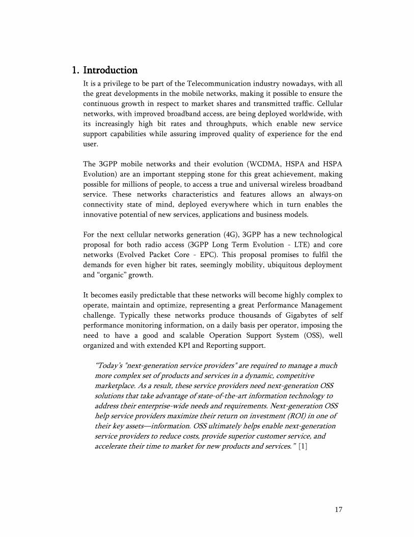
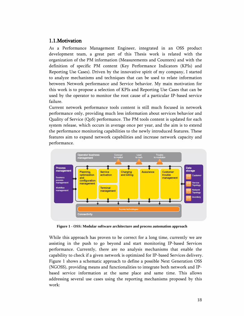
Figure 1 - OSS: Modular software architecture and process automation approach
While this approach has proven to be correct for a long time, currently we are
assisting in the push to go beyond and start monitoring IP-based Services
performance. Currently, there are no analysis mechanisms that enable the
capability to check if a given network is optimized for IP-based Services delivery.
Figure 1 shows a schematic approach to define a possible Next Generation OSS
(NGOSS), providing means and functionalities to integrate both network and IP-
based service information at the same place and same time. This allows
addressing several use cases using the reporting mechanisms proposed by this
work:
19
• Monitor Service Level Agreements fulfillment;
• Answer IP-based service subscriber complaints;
• Monitor and optimize operator own services and network;
• Forecast future service delivery requirements and network capacity
expansion.
This work proposes a new approach in performance monitoring that relates the IP-
based Service QoS performance with the network performance. This allows
identifying which layer is contributing for the lack of performance and what are the
corrective measures to take.

20
1111....2222.... ObjectivesObjectivesObjectivesObjectives
IP Converged networks are becoming a reality, with more and more networks
extending the IP delivery support. Cellular networks have been definitely
contributing in a decisive way for this accomplishment, with the latest
evolutions (HSDPA, HSUPA, HSPA+ and soon LTE) offering a great coverage of
cellular broadband access. The effective support of IP connectivity through
mobile broadband opens the opportunity to offer new bouquet of diverse and
rich multimedia services, ranging from entertainment based services like Gaming
and Mobile TV to some more business oriented services like Machine-2-Machine
(M2M) communication and Web Conferencing.
This new reality brings new challenges to network operational, maintenance and
optimization procedures, since the shift from Circuit Switched (CS) Voice
optimized networks to all kind of IP-Services optimized networks, increases the
number of optimization variables and thus the process complexity. The questions
to be answered are the following: Do we have all the tools in place that can tell
us how current network performance is influencing a particular IP session
performance? Can we relate network and service statistics in a way that indicate
to us if a particular network is suitable for that service delivery? Can we tell,
prior to a new service deployment, if the network is suitable as it is? And if not,
what should be the improvements to be done?
This work main objective is to answer these questions by proposing a reporting
concept that relates information from two distinct but inter-dependent layers:
Network Performance and IP-Based Service Performance. The intention is to
select for each layer the most important KPIs and define analysis use cases that
propose a workflow for performance monitoring and identify the correct
measures to apply whenever needed. In the end, the results will show how these
layers influence one another.
21
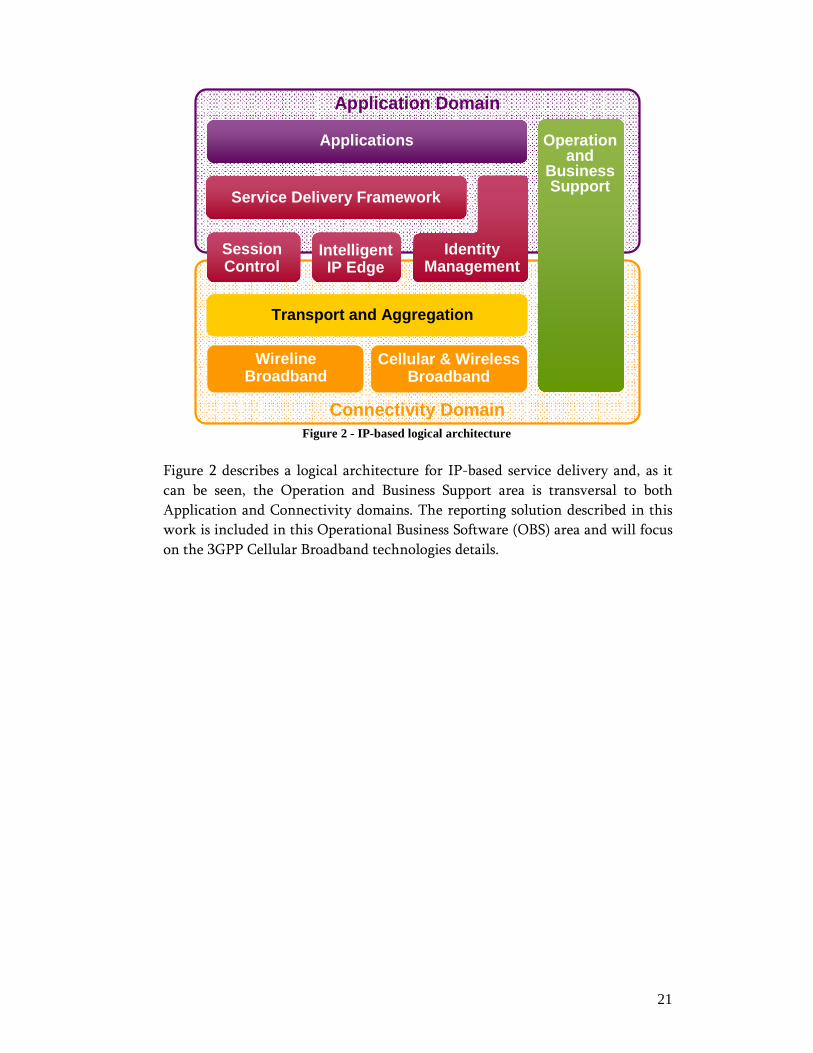
Figure 2 - IP-based logical architecture
Figure 2 describes a logical architecture for IP-based service delivery and, as it
can be seen, the Operation and Business Support area is transversal to both
Application and Connectivity domains. The reporting solution described in this
work is included in this Operational Business Software (OBS) area and will focus
on the 3GPP Cellular Broadband technologies details.
Connectivity Domain
Service Delivery Framework
Applications
SessionControl
IdentityManagement
Application Domain
Transport and Aggregation
IntelligentIP Edge
WirelineBroadband
Cellular & WirelessBroadband
Operationand
BusinessSupport
22
1111....3333.... Contributions of the ThesisContributions of the ThesisContributions of the ThesisContributions of the Thesis
The work developed accomplishes the major part of the proposed objectives and,
as a result, its main contributions are:
• The proposal of a new PM Reporting feature that allows enabling IP-
based QoS statistics monitoring related with Network Performance
Monitoring. This feature will be integrated in Nokia Siemens
Networks Reporting products commercial releases;
• The evaluation of real time IP-based Service (VoIP and IPTV) over
HSPA, being valuable for the service key statistics identification;
• The work develop within this thesis, particularly the identification of
the network performance monitoring architecture, layers and KPIs is
part of a published article:
� Miguel Almeida, Rui Inácio, Susana Sargento, “Cross Layer
Design Approach for Performance Evaluation of
Multimedia Contents”, 2nd International Workshop on
Cross Layer Design (IWCLD 2009), Mallorca (Spain), June
2009.
23
1111....4444.... Organization of the ThesisOrganization of the ThesisOrganization of the ThesisOrganization of the Thesis
The present thesis is organized as follows:
• Chapter 2 provides an overview about this work related areas such as
Network Management and 3GPP Networks. This work main goal is to
provide a new concept of network and IP-based service performance
monitoring to be applied to 3GPP operational support, and therefore,
this chapter highlights all the relevant matters for the development of
this study.
• Chapter 3 introduces the details related with this work concept
proposal, describes the proposed architecture, identifies the
performance data sources, introduces the data modeling processes,
details the relevant Key Performance Indicators and presents the new
reporting concept describing some relevant use cases.
• Chapter 4 discusses the simulation environment and simulated results
for a VoIP service running on top of a 3GPP network combining
UMTS R99 and HSPA elements.
• Chapter 5 presents the final conclusions taken from this work and
identifies some possible future work.

24
2222.... BackgroundBackgroundBackgroundBackground
This chapter introduces the several concepts that are fundamental for the
understanding of this work. Section 2.1 discusses the Network Management
thematic detailing the Telecommunication Management Network concept,
providing an insight about its objectives and structure, as well as briefly describes
some of the most used performance monitoring techniques. Section 2.2 introduces
the cellular packet switching networks, detailing its architecture, network elements,
functionalities and procedures. Section 2.3 introduces in some detail the 3GPP
UMTS High-Speed Packet Access technology, detailing the enhancements
introduced when compared with UMTS R99 WCDMA technology. This section first
provides a brief introduction to UMTS R99 data transmission functionalities, then
detailing the HSDPA and HSUPA technological improvements, and the main
characteristics that enable HSPA as a suitable technology for real-time IP-based
service delivery. Section 2.4 provides a brief introduction to the 3GPP Long Term
Evolution proposal that aims to be the main 4G technology. The last Section 2.5
summarizes the most important contents mentioned in this chapter.
2222....1111.... Network ManagementNetwork ManagementNetwork ManagementNetwork Management
“An essential question when designing the network architecture is how to
manage and monitor the network’s overall operation, and remove flaws from the
network when they occur. In general, network management can be perceived as
a service that employs a variety of methods and tools, applications, and devices
to enable the network operator to monitor and maintain the entire network. For
a typically centralized mobile network, network management means the ability
to control and monitor the entire network from a specific location and, possibly,
remotely. The rapid universal growth of mobile networks has made the role of
the network management a key feature that should be carefully taken into
account early in the design process of network architecture. In particular, the
basic functionality of networks should provide operators with the ability to
control and maintain their networks and services.” [2]
Several efforts, from different standardization organizations, have been
developed to standardize a common network management model. The
International Standard Organization (ISO) proposes a management framework [3]
that proposes to control and monitor the use of network resources by defining a
model which provides data storage and processing capabilities that can relate the
performance of the different functional parts of the network. This model defines
that the ultimate management decision is of Human beings responsibility,
although the responsibilities may be delegated to the system automated processes.
The OSI management functional areas are:
• Fault Management;

25
• Accounting Management;
• Configuration Management;
• Performance Management;
• Security Management.
The OSI Model defines functional mechanisms for each of these areas, being
these mechanisms and related objects generic to more than one of these areas.
Important to mention is that the OSI model is the reference of some network
management protocol such as Common Management Information
Services/Common Management Information Protocol (CMIS/CMIP) [4] and
Simple Network Management Protocol (SNMP) [5] [6].
International Telecommunication Union – Telecom Standardization (ITU-T) also
defined a network management model, the Telecommunications Management
Networks (TMN) [7]. This has become the dominant network management
concept within the telecommunications world, serving as a reference for all the
OSS system vendors.
2222....1111....1111.... TMN Logical ModelTMN Logical ModelTMN Logical ModelTMN Logical Model
This work assumes that all the referred Operational Support Systems are
based on the Telecommunications Management Networks (TMN) concept.
The TMN concept was defined by the International Telecommunications
Union – Telecommunications Service Sector (ITU-T) as an infrastructure to
support management and deployment heterogeneous operating systems and
telecommunication networks. TMN proposes a framework of software
applications and procedures for operating and managing networks in a
flexible, scalable, reliable, inexpensive to use and easy to enhance process.
The following layers are defined:
Business Management Layer (BML)Business Management Layer (BML)Business Management Layer (BML)Business Management Layer (BML) – high-level layer that focus on providing
mechanisms and procedures that allow to: define business goals, do business
planning, product planning, service planning, business agreements, etc. This
layer is close related with financial metrics (like budgeting, revenue, OPEX,
CAPEX), with legal arrangements and security issues.
Service Management Layer (SML)Service Management Layer (SML)Service Management Layer (SML)Service Management Layer (SML) – this layer provides information that
allows coordinating the interaction between services and service providers,
interfaces with partner companies, customers and vendors. SML is
responsible for collecting and analyze QoS metrics to insure that Service
Level Agreement (SLA), between network operator and service provider, is
being fulfilled.
26
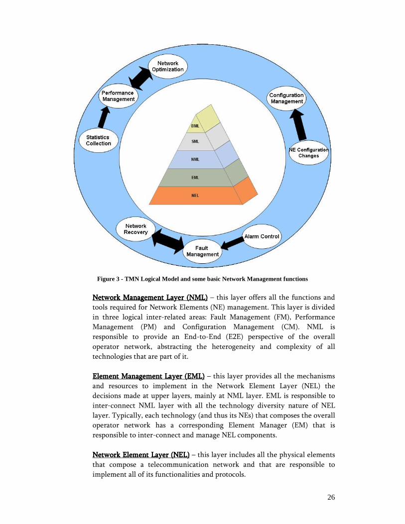
Figure 3 - TMN Logical Model and some basic Network Management functions
NetworkNetworkNetworkNetwork Management Layer (NML) Management Layer (NML) Management Layer (NML) Management Layer (NML) – this layer offers all the functions and
tools required for Network Elements (NE) management. This layer is divided
in three logical inter-related areas: Fault Management (FM), Performance
Management (PM) and Configuration Management (CM). NML is
responsible to provide an End-to-End (E2E) perspective of the overall
operator network, abstracting the heterogeneity and complexity of all
technologies that are part of it.
Element Management Layer (EML)Element Management Layer (EML)Element Management Layer (EML)Element Management Layer (EML) – this layer provides all the mechanisms
and resources to implement in the Network Element Layer (NEL) the
decisions made at upper layers, mainly at NML layer. EML is responsible to
inter-connect NML layer with all the technology diversity nature of NEL
layer. Typically, each technology (and thus its NEs) that composes the overall
operator network has a corresponding Element Manager (EM) that is
responsible to inter-connect and manage NEL components.
Network Element Layer (NEL)Network Element Layer (NEL)Network Element Layer (NEL)Network Element Layer (NEL) – this layer includes all the physical elements
that compose a telecommunication network and that are responsible to
implement all of its functionalities and protocols.
27
2222....1111....2222.... Performance Management TechniquesPerformance Management TechniquesPerformance Management TechniquesPerformance Management Techniques
Performance Management covers a wide range of areas and functions;
therefore, different techniques must be deployed. These techniques range
from drive-tests, on-line monitoring of real-time performance metrics, to
trend monitoring based on historical and aggregated data.
For each of these techniques there is a software tool type that is most
adequate for the specific technique requirements. For instance, a drive-test
tool must be adequate to collect the signaling messages that are transferred in
the network radio interface in order to trace the network failures. This type
of analysis is very specific, detailed, geographically limited and expensive,
therefore its occurrence tends to be scarce, and is typically performed only
when PM counters do not provide enough detail.
Other tools that rely mostly on PM data generated and collected from
network elements, tend to have a wide and frequent use. This type of data
can be used to perform on-line network monitoring that is characterized by
the small data granularity which, in case of failure, enables the ability to act
immediately upon the problem. Another important analysis performed using
PM counters is the trend analysis, which can serve the intents of both
Network Planning and Optimization Engineers, Marketing, Administration
and Business Development people.
A PM Reporting tool is the key application in providing all this information,
as its capabilities allow manipulate the network PM data to directly answer
all these use cases. The PM data can be more or less summarized and
relations can be established between performance indicators in a way that
logically can provide answers for question coming from a multitude of
different perspectives.
Although existing performance techniques work very well for network
performance monitoring, the same is not applied to service layer QoS
monitoring. The currently available systems depend on the metrics collected
by the network elements in their self-monitoring procedures, which is a
problem when it comes to monitor IP-based services QoS performance. The
challenge of monitoring IP-based services over Cellular networks is that in
the IP service layer path there are no network elements to retrieve
performance data. One of the innovative factors of this work is to propose the
usage of new IT techniques, like deep packet inspection, that extend the
scope of the performance data gathered from the network to focus on IP-
based service layer statistics.
This new data sources associated with performance management techniques
that historically have proven to be effective will drive to a broad bouquet of
monitoring solutions. For instance, there are already some tools that provide
the ability to run drive tests at the application layer, which enables the
28
capability to collect and analyze Quality of Experience statistics (QoE). In the
other hand, there are already some solutions that address the on-line
monitoring of IP-based Service Sessions that allow to detect almost
instantaneously degradations in the session QoS performance.
However these solutions do not answer the questions that drove this work,
mainly related with how network and service layer performance influencing
each other behavior. This work proposes a new reporting approach that
relates, in a cross-layer fashion, the service metrics with the network layer
indicators.
2222....2222.... Packet Switched NetworksPacket Switched NetworksPacket Switched NetworksPacket Switched Networks
Although Universal Mobile Telecommunication System (UMTS) Core Network
(CN) can be constituted by both Packet-Switch (PS) and Circuit-Switched (CS)
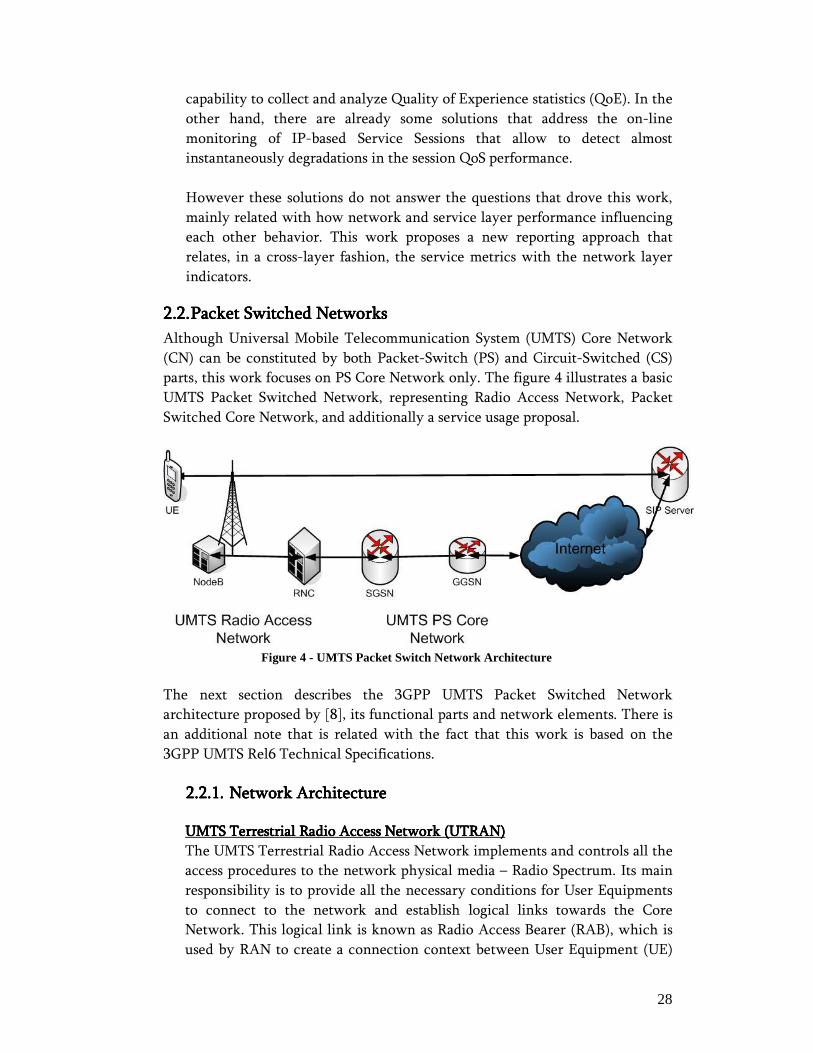
parts, this work focuses on PS Core Network only. The figure 4 illustrates a basic
UMTS Packet Switched Network, representing Radio Access Network, Packet
Switched Core Network, and additionally a service usage proposal.
Figure 4 - UMTS Packet Switch Network Architecture
The next section describes the 3GPP UMTS Packet Switched Network
architecture proposed by [8], its functional parts and network elements. There is
an additional note that is related with the fact that this work is based on the
3GPP UMTS Rel6 Technical Specifications.
2222....2222....1111.... Network ArchitectureNetwork ArchitectureNetwork ArchitectureNetwork Architecture
UMTS Terrestrial Radio Access Network (UTRAN)UMTS Terrestrial Radio Access Network (UTRAN)UMTS Terrestrial Radio Access Network (UTRAN)UMTS Terrestrial Radio Access Network (UTRAN)
The UMTS Terrestrial Radio Access Network implements and controls all the
access procedures to the network physical media – Radio Spectrum. Its main
responsibility is to provide all the necessary conditions for User Equipments
to connect to the network and establish logical links towards the Core
Network. This logical link is known as Radio Access Bearer (RAB), which is
used by RAN to create a connection context between User Equipment (UE)
29
and CN. RAB implements, at RAN side, all the E2E QoS call related
requirements, defined by CN.
In order to be capable of supporting RAB QoS requirements for each call,
RAN has the responsibility to manage all the radio resources available and
system capacity usage. As it is commonly known, the radio resources are
scarce which makes Radio Resource Management (RRM) function as one of
RAN’s most important features.
UTRAN is constituted by two major network elements: Node B and Radio
Network Controller (RNC).
Node BNode BNode BNode B
Node B is the radio access point of UTRAN; its main responsibility is to
implement the Uu radio physical interface, allowing that UE links to the
network and enabling data transmission from and towards the network. Node
B interfaces RNC through Iub interface.
Radio Network Controller (RNC)Radio Network Controller (RNC)Radio Network Controller (RNC)Radio Network Controller (RNC)
The RNC is the brain of UTRAN. RNC is the responsible element for the
control of radio resources.
Functions that are performed by the RNC include:
• Iub transport resources management;
• Traffic Management of common and shared channels;
• Macro diversity combining/splitting of data streams
transmitted over several Node Bs;
• Soft Handover control;
• Power Control;
• Admission Control;
• Channelization Code allocation;
• Handover Control;
• Packet Scheduling.
RAN InterfacesRAN InterfacesRAN InterfacesRAN Interfaces
There are three major transmission interfaces internal to RAN part: Iu, Iur
and Iub interfaces.
Iu interface is responsible to connect RNC to corresponding Core Network
element (SGSN). This interface is used to carry both Control and User Plane
information. The control plane protocol stack consists of Radio Access
Network Application Part (RANAP) and is used to control the Radio
Network Layer. The Iu User Plane part is responsible for the user data
transmission between RAN and CN.
30
Iur interface is responsible for the communication between adjacent RNCs.
This interface was initially designed to support inter-RNC soft handover;
however, more functions were added afterwards, like the support of inter-
RNC mobility, dedicated and common channel traffic transmission and
global resource management support.
Iub interface is responsible for the communication between RNC and Node B;
it supports both Control Plane and User Plane protocol stack. The control
plane protocol stack consists of Node B Application Part (NBAP). The Iub
User Plane part consists of transmitting Frame Protocol Packets that
transport MAC Layer Protocol Data Unit (PDU) related to radio dedicated
and shared channels.
UMTS Packet Switched Core Network (UMTS PS CN)UMTS Packet Switched Core Network (UMTS PS CN)UMTS Packet Switched Core Network (UMTS PS CN)UMTS Packet Switched Core Network (UMTS PS CN)
Packet Switched Core Network plays a central role in UMTS system by
providing means for subscriber authentication, mobility management, session
management, packet routing, charging, etc. In order to implement these
functionalities, there were defined two major network elements: Serving
GPRS Support Node (SGSN) and Gateway GPRS Support Node (GGSN).
Serving GPRS Support Node (SGSN)Serving GPRS Support Node (SGSN)Serving GPRS Support Node (SGSN)Serving GPRS Support Node (SGSN)
SGSN is the UMTS PS CN dedicated node for authentication and mobility
management. This node serves as point of connection between the access
network and the packet routing node by creating a mobility management
context, which keeps track of UE Routing Area of specific cell, allowing to
always delivering the packets to the UE regardless of its mobility. Its task
includes:
• Packet transfer between RNC and GGSN;
• Mobility Management (attach/detach and location
management);
• Logical Link Management;
• Authentication;
• Charging functions.
Gateway GPRS Support Node (GGSN)Gateway GPRS Support Node (GGSN)Gateway GPRS Support Node (GGSN)Gateway GPRS Support Node (GGSN)
GGSN is the UMTS PS CN gateway towards external IP networks such as
public Internet, other mobile service provider’s GPRS services, or enterprise
intranets. GGSN maintains routing information necessary to tunnel the PDU
data towards a SGSN serving a particular UE. To be able to route information
from external networks towards the end user, GGSN holds information about
the subscriber like: IMSI number, Packet Data Protocol (PDP) addresses, UE
location information and serving SGSN information.
31
Data coming from SGSN in direction to an external network is converted by
GGSN from GTP-U packets into IP packets and then transmitted. External
access is accomplished through an entity called Access Point Name (APN)
that is defined and implemented through GGSN. APN identifies the external
networks or service servers that are accessed by subscribers via GGSN. For
each GGSN there can be several thousands of defined APN.
2222....2222....2222.... Packet Session Establishment ProcedurePacket Session Establishment ProcedurePacket Session Establishment ProcedurePacket Session Establishment Procedure
This section explains all the fundamental steps for the establishments of a PS
session, detailing the message flows that occur in this procedure. This session
setup flow is composed by: Radio Resource Control (RRC) Connection Setup
Procedure defined in [9]; GPRS Mobility Management control defined in [10];
Radio Access Bearer Assignment Procedure described in [11]; Radio Bearer
Reconfiguration procedure defined in [9] and Radio Link Reconfiguration
procedure described in [12].
This call flow description begins assuming that the UE is in RRC Idle Mode
(UE is camped in a given cell). Figure 5 shows the control message flow for
the call setup initiation process. UE starts to transmit a RRC connection
request message to the RNC, through transport Radio Access Channel
(RACH), which is encapsulated by the Physical Random Access Channel
(PRACH).
This RRC connection request message is relatively small requiring only a
single transport block transmitted using a 20ms Transmission Time Interval
(TTI) and the RLC protocol in transparent mode. The RRC connection
requested message can always be retransmitted, if necessary.
Once the RNC receives this RRC Connection Request message, it requests a
Radio Link at the relevant Node B using NBAP signaling (NBAP: Radio link
setup request/response messages). Node B starts to transmit a Dedicated
Physical Control Channel (DPCCH) for the new Radio Link (RL). The RNC
then reserves a set of Iub resources, using Access Link Control Application
Part (ALCAP) Establish request/confirm messages.
Then, the RNC answers to the first RRC connection request message sent by
the UE, using a RRC connection setup message, transmitted over Forward
Access Channel (FACH). This RRC connection setup message is relatively
large and requires seven transport blocks. These transport blocks have a size
of 168 bits which are transmitted using a 10ms TTI and unacknowledged
mode RLC. The block set size is typically defined such as two transport
blocks can be sent per 10ms TTI. If the UE is in a poor coverage area, then it
is possible that it did not receive one or more of the RRC connection setup
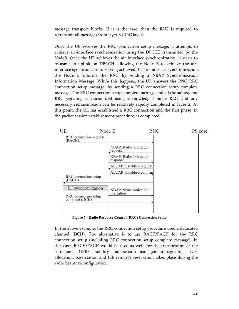
32
message transport blocks. If it is the case, then the RNC is required to
retransmit all messages from layer 3 (RRC layer).
Once the UE receives the RRC connection setup message, it attempts to
achieve air-interface synchronization using the DPCCH transmitted by the
NodeB. Once the UE achieves the air-interface synchronization, it starts to
transmit in uplink on DPCCH, allowing the Node B to achieve the air-
interface synchronization. Having achieved the air-interface synchronization,
the Node B informs the RNC by sending a NBAP Synchronization
Information Message. While this happens, the UE answers the RNC RRC
connection setup message, by sending a RRC connection setup complete
message. The RRC connection setup complete message and all the subsequent
RRC signaling is transmitted using acknowledged mode RLC, and any
necessary retransmission can be relatively rapidly completed in layer 2. At
this point, the UE has established a RRC connection and the first phase, in
the packet session establishment procedure, is completed.
Figure 5 - Radio Resource Control (RRC) Connection Setup
In the above example, the RRC connection setup procedure used a dedicated
channel (DCH). The alternative is to use RACH/FACH for the RRC
connection setup (including RRC connection setup complete message). In
this case, RACH/FACH would be used as well, for the transmission of the
subsequent GPRS mobility and session management signaling. DCH
allocation, base station and Iub resource reservation takes place during the
radio bearer reconfiguration.

33
The second phase of a Mobile-Originated (MO) Packet-Switched (PS) data
session establishment procedure involves GPRS Mobility Management
(GMM) signaling with the core network. Figure 6 shows the GMM control
message flow exchanged between the involved NEs.
Figure 6 - GPRS mobility management
The UE sends a GPRS attach request message to the PS core through the RNC.
The RNC relays the content of the message to the core network using a
RANAP Initial UE Message. The RANAP message is combined with a
Signaling Connection Control Part (SCCP) connection request message
which is utilized to request the Iu signaling resources. The core network
answers to the RNC with a SCCP connection confirm message to
acknowledge that a signaling connection has been established across the Iu
interface. The core network then completes the security mode procedure.
There may be also a requirement to complete the authentication and
ciphering procedure, which can be configured if it is needed for all the
connections, or just for a specific percentage of them. Once the security
mode is completed, the core network is able to send the GPRS attach accept
message, becoming the UE registered for packet-switched services.
The third phase of Mobile Originated Packet Switched data session involves
GPRS Session Management (GSM) and RAB assignment signaling messages,
which are shown in Figure 7.
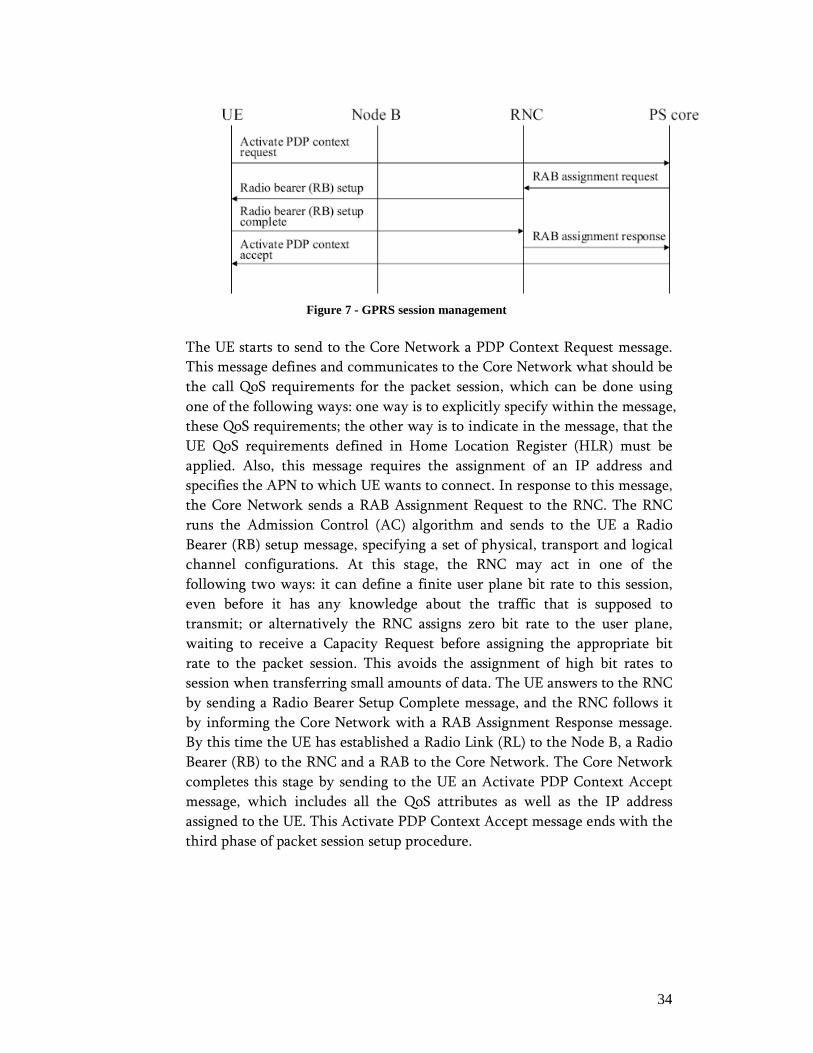
34
Figure 7 - GPRS session management
The UE starts to send to the Core Network a PDP Context Request message.
This message defines and communicates to the Core Network what should be
the call QoS requirements for the packet session, which can be done using
one of the following ways: one way is to explicitly specify within the message,
these QoS requirements; the other way is to indicate in the message, that the
UE QoS requirements defined in Home Location Register (HLR) must be
applied. Also, this message requires the assignment of an IP address and
specifies the APN to which UE wants to connect. In response to this message,
the Core Network sends a RAB Assignment Request to the RNC. The RNC
runs the Admission Control (AC) algorithm and sends to the UE a Radio
Bearer (RB) setup message, specifying a set of physical, transport and logical
channel configurations. At this stage, the RNC may act in one of the
following two ways: it can define a finite user plane bit rate to this session,
even before it has any knowledge about the traffic that is supposed to
transmit; or alternatively the RNC assigns zero bit rate to the user plane,
waiting to receive a Capacity Request before assigning the appropriate bit
rate to the packet session. This avoids the assignment of high bit rates to
session when transferring small amounts of data. The UE answers to the RNC
by sending a Radio Bearer Setup Complete message, and the RNC follows it
by informing the Core Network with a RAB Assignment Response message.
By this time the UE has established a Radio Link (RL) to the Node B, a Radio
Bearer (RB) to the RNC and a RAB to the Core Network. The Core Network
completes this stage by sending to the UE an Activate PDP Context Accept
message, which includes all the QoS attributes as well as the IP address
assigned to the UE. This Activate PDP Context Accept message ends with the
third phase of packet session setup procedure.
35
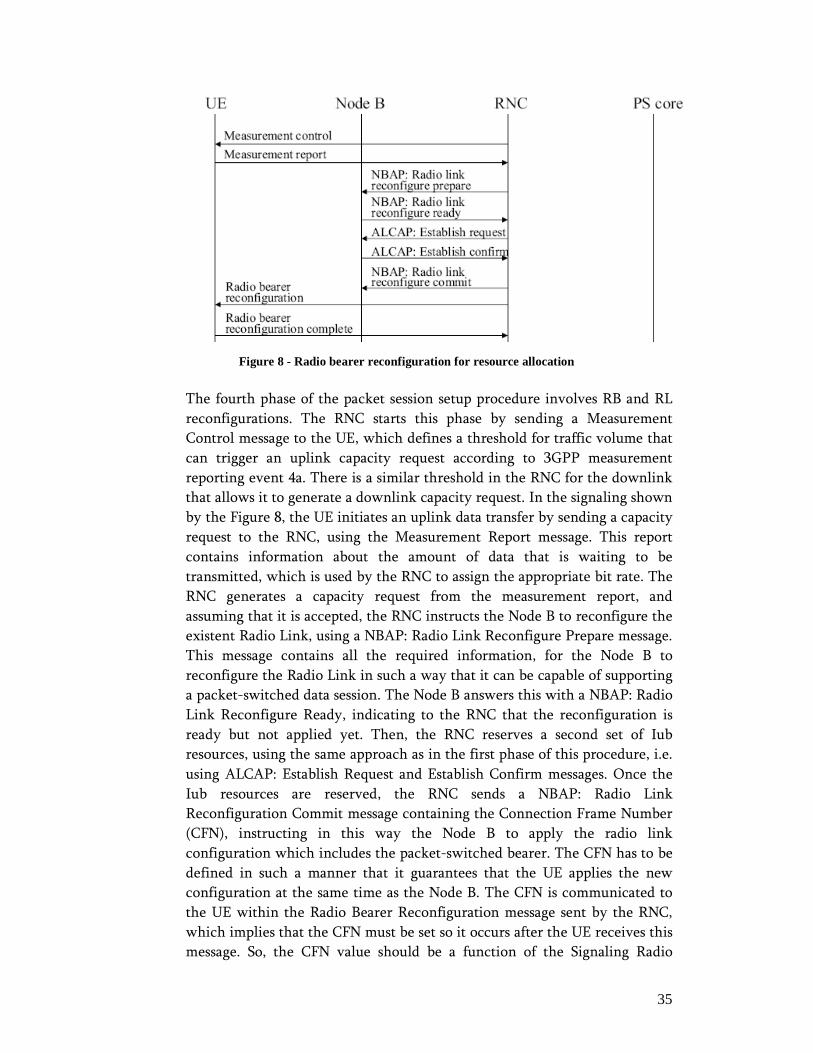
Figure 8 - Radio bearer reconfiguration for resource allocation
The fourth phase of the packet session setup procedure involves RB and RL
reconfigurations. The RNC starts this phase by sending a Measurement
Control message to the UE, which defines a threshold for traffic volume that
can trigger an uplink capacity request according to 3GPP measurement
reporting event 4a. There is a similar threshold in the RNC for the downlink
that allows it to generate a downlink capacity request. In the signaling shown
by the Figure 8, the UE initiates an uplink data transfer by sending a capacity
request to the RNC, using the Measurement Report message. This report
contains information about the amount of data that is waiting to be
transmitted, which is used by the RNC to assign the appropriate bit rate. The
RNC generates a capacity request from the measurement report, and
assuming that it is accepted, the RNC instructs the Node B to reconfigure the
existent Radio Link, using a NBAP: Radio Link Reconfigure Prepare message.
This message contains all the required information, for the Node B to
reconfigure the Radio Link in such a way that it can be capable of supporting
a packet-switched data session. The Node B answers this with a NBAP: Radio
Link Reconfigure Ready, indicating to the RNC that the reconfiguration is
ready but not applied yet. Then, the RNC reserves a second set of Iub
resources, using the same approach as in the first phase of this procedure, i.e.
using ALCAP: Establish Request and Establish Confirm messages. Once the
Iub resources are reserved, the RNC sends a NBAP: Radio Link
Reconfiguration Commit message containing the Connection Frame Number
(CFN), instructing in this way the Node B to apply the radio link
configuration which includes the packet-switched bearer. The CFN has to be
defined in such a manner that it guarantees that the UE applies the new
configuration at the same time as the Node B. The CFN is communicated to
the UE within the Radio Bearer Reconfiguration message sent by the RNC,
which implies that the CFN must be set so it occurs after the UE receives this
message. So, the CFN value should be a function of the Signaling Radio
36
Bearer rate, i.e. a shorter activation time can be used with the 13.6-kbps than
with the 3.4-kbps signaling bit rate, and thus this must be taken into
consideration. Plus, some margin should be allowed for L2 retransmissions
and processing time, thus it is common that the RNC includes an additional
parameter that defines a configurable time offset for the CFN.
Once the CFN occurs and the new configuration has become active, the UE
answers with the Radio Bearer Reconfiguration Complete Message. This
message and the subsequent signaling are transmitted across the air-interface
using the 3.4 kbps bit rate, even if the 13.6 kbps bit rate had been applied
previously. The UE is now configured with a finite user plane bit rate
towards the PS core network and is ready to transfer data.
2222....3333.... HighHighHighHigh----Speed Packet AccessSpeed Packet AccessSpeed Packet AccessSpeed Packet Access
HSPA is a term used to denominate two major technological enhancements to
UMTS RAN technology: High-Speed Downlink Packet Access and High-Speed
Uplink Packet Access. These new technological proposals were pushed by the
increasingly need of data throughput demand.
2222....3333....1111.... UMTS R99 before HSPAUMTS R99 before HSPAUMTS R99 before HSPAUMTS R99 before HSPA
Although there are major achievements in HSDPA and HSUPA
enhancements, Packet data transmission is supported right from the initial
deployments of UMTS networks. The following downlink radio channels are
available since UMTS R99 [13]:
• Dedicated Channel (DCH)Dedicated Channel (DCH)Dedicated Channel (DCH)Dedicated Channel (DCH)::::
o Transmitted over the Downlink Dedicated Physical
Channel (DDPCH);
o Maximum bit rate of 2 Mbps;
o Can be used for any kind of service that requires QoS
guarantees;
o Suitable for medium or large amount of data
transmission;
o Reserves enough code capacity for the support of
connection’s required maximum bit rate;
o Reserved codes are dedicated to a specific connection
only;
o Supports Fast Power Control;
o Supports soft handover.
• Downlink Shared Channel (DSCH):Downlink Shared Channel (DSCH):Downlink Shared Channel (DSCH):Downlink Shared Channel (DSCH):
o Uses dynamic variable spreading factor allocation;
o Mainly designed to transfer bursty packet data;

37
o Suitable for medium or large amount of data
transmission;
o Code resources are shared between all the connections
using a time division approach;
o Supports single-code and multi-code transmission;
o Does not support Soft Handover;
o Supports Fast Power Control;
o It was removed from 3GPP specifications since the
introduction of High-Speed DSCH (HS-DSCH) in
UMTS Release 5.
• Forward Access Channel (FACH):Forward Access Channel (FACH):Forward Access Channel (FACH):Forward Access Channel (FACH):
o Transmitted over the Secondary Common Control
Physical Channel (S-CCPCH);
o Uses a fixed Spreading Factor;
o Does not support Soft Handover;
o Does not support power control;
o Mainly designed to transfer bursty packet data;
o Suitable for small amount of data transmission;
2222....3333....2222.... HighHighHighHigh----Speed Downlink Packet Access (HSDPA)Speed Downlink Packet Access (HSDPA)Speed Downlink Packet Access (HSDPA)Speed Downlink Packet Access (HSDPA)
HSDPA was introduced in 3GPP Release 5 [14] and represents for WCDMA
technology a major advance when compared with Release 99 capabilities.
Although UMTS Release 99 (R99) already offers some methods for packet
transmission over WCDMA air interface in downlink direction, the
improvements introduced by HSDPA enhance substantially the downlink
packet data throughput, which is fundamental for the support of rich
multimedia content oriented services.
The required techniques to achieve higher data rates delivery and reduced
delay are to implement Link Adaptation control closer to air interface and
Physical Layer (L1) retransmission combining; HSDPA implements some
architectural changes. A new user data transport channel is introduced,
High-Speed Downlink Shared Channel (HS-DSCH), packet scheduling and
link adaptation are conducted in the Node B according to the active
scheduling algorithm and user priority handling mechanism. Channel quality
is estimated by the Node B based on Channel Quality Indication (CQI)
reports, power control, acknowledgment/non-acknowledgment (ACK/NACK)
ratio and specific HSDPA user feedback.
HS-DSCH transport channel characteristics:
• Does not support soft-handover
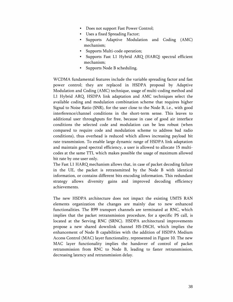
38
• Does not support Fast Power Control;
• Uses a fixed Spreading Factor;
• Supports Adaptive Modulation and Coding (AMC)
mechanism;
• Supports Multi-code operation;
• Supports Fast L1 Hybrid ARQ (HARQ) spectral efficient
mechanism;
• Supports Node B scheduling.
WCDMA fundamental features include the variable spreading factor and fast
power control; they are replaced in HSDPA proposal by Adaptive
Modulation and Coding (AMC) technique, usage of multi-coding method and
L1 Hybrid ARQ. HSDPA link adaptation and AMC techniques select the
available coding and modulation combination scheme that requires higher
Signal to Noise Ratio (SNR), for the user close to the Node B, i.e., with good
interference/channel conditions in the short-term sense. This leaves to
additional user throughputs for free, because in case of good air interface
conditions the selected code and modulation can be less robust (when
compared to require code and modulation scheme to address bad radio
conditions), thus overhead is reduced which allows increasing payload bit
rate transmission. To enable large dynamic range of HSDPA link adaptation
and maintain good spectral efficiency, a user is allowed to allocate 15 multi-
codes at the same TTI, which makes possible the usage of maximum allowed
bit rate by one user only.
The Fast L1 HARQ mechanism allows that, in case of packet decoding failure
in the UE, the packet is retransmitted by the Node B with identical
information, or contains different bits encoding information. This redundant
strategy allows diversity gains and improved decoding efficiency
achievements.
The new HSDPA architecture does not impact the existing UMTS RAN
elements organization the changes are mainly due to new enhanced
functionalities. The R99 transport channels are terminated at RNC, which
implies that the packet retransmission procedure, for a specific PS call, is
located at the Serving RNC (SRNC). HSDPA architectural improvements
propose a new shared downlink channel HS-DSCH, which implies the
enhancement of Node B capabilities with the addition of HSDPA Medium
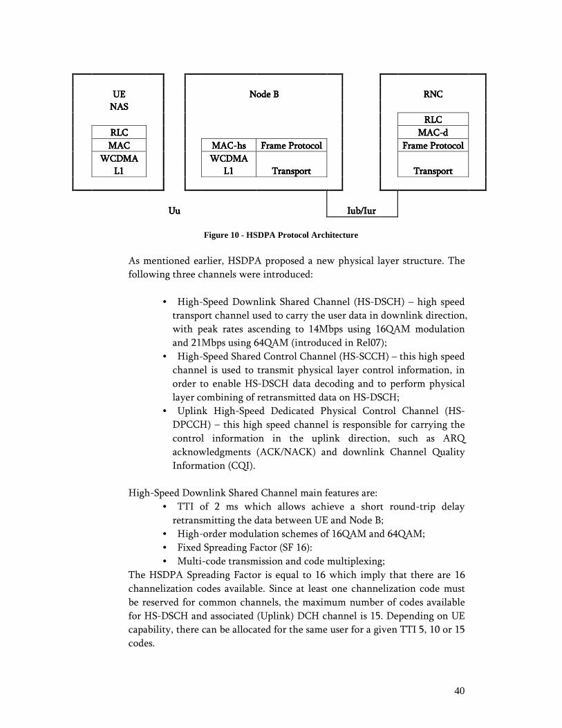
Access Control (MAC) layer functionality, represented in Figure 10. The new
MAC layer functionality implies the handover of control of packet
retransmission from RNC to Node B, leading to faster retransmission,
decreasing latency and retransmission delay.

39
The following figure shows the packet retransmission handling both in R99
and HSDPA systems, in the case where the Serving RNC and Controlling
RNC are the same.
Figure 9 - Packet Retransmission Control: Rel99 versus HSDPA
In the HSDPA architecture, the RNC still retains the control of the Radio
Link Control functions, which in case, for instance, of exceeding the number
of maximum HS-DSCH retransmissions from Node B, it will take care of
retransmitting the lost packet.
The new Node B MAC functionality is responsible for the HARQ functions,
scheduling and priority handling. Ciphering is still done in the RLC layer, i.e.
at the RNC, to ensure that the ciphering mask stays identical through the
entire transmission/retransmission process, enabling this way the combining
of retransmissions.
The type of scheduling to be implemented in the Node B is not defined by
3GPP standards, just few parameters are addressed, such as discard timer or
priority scheduling indication that can be used by RNC to control the
handling of an individual user. The scheduler type has a great impact on the
system performance thus impacting the Quality of Service (QoS). This is a
key factor for equipment vendor differentiation and influences the network
operator choice in closing deals or not.
40
UEUEUEUE Node BNode BNode BNode B RNCRNCRNCRNC
NASNASNASNAS
RLCRLCRLCRLC
RLCRLCRLCRLC MACMACMACMAC----dddd
MACMACMACMAC MACMACMACMAC----hshshshs Frame ProtocolFrame ProtocolFrame ProtocolFrame Protocol Frame ProtocolFrame ProtocolFrame ProtocolFrame Protocol
WCDMA WCDMA WCDMA WCDMA
L1L1L1L1
WCDMA WCDMA WCDMA WCDMA
L1L1L1L1 TransportTransportTransportTransport TransportTransportTransportTransport
UuUuUuUu Iub/IurIub/IurIub/IurIub/Iur
Figure 10 - HSDPA Protocol Architecture
As mentioned earlier, HSDPA proposed a new physical layer structure. The
following three channels were introduced:
• High-Speed Downlink Shared Channel (HS-DSCH) – high speed
transport channel used to carry the user data in downlink direction,
with peak rates ascending to 14Mbps using 16QAM modulation
and 21Mbps using 64QAM (introduced in Rel07);
• High-Speed Shared Control Channel (HS-SCCH) – this high speed
channel is used to transmit physical layer control information, in
order to enable HS-DSCH data decoding and to perform physical
layer combining of retransmitted data on HS-DSCH;
• Uplink High-Speed Dedicated Physical Control Channel (HS-
DPCCH) – this high speed channel is responsible for carrying the
control information in the uplink direction, such as ARQ
acknowledgments (ACK/NACK) and downlink Channel Quality
Information (CQI).
High-Speed Downlink Shared Channel main features are:
• TTI of 2 ms which allows achieve a short round-trip delay
retransmitting the data between UE and Node B;
• High-order modulation schemes of 16QAM and 64QAM;
• Fixed Spreading Factor (SF 16):
• Multi-code transmission and code multiplexing;
The HSDPA Spreading Factor is equal to 16 which imply that there are 16
channelization codes available. Since at least one channelization code must
be reserved for common channels, the maximum number of codes available
for HS-DSCH and associated (Uplink) DCH channel is 15. Depending on UE
capability, there can be allocated for the same user for a given TTI 5, 10 or 15
codes.

41
Code multiplexing allows that different UEs use the same HS-DSCH (or same
channelization code) channel to transmit data at different TTI, which
contributes to improved spectral efficiency.
HS-DSCH modulation can be originally of 16QAM or, since Rel07, of
64QAM. The use of these modulation schemes, associated with multi-code
technique, increases significantly the available user data rates.
2222....3333....3333.... HighHighHighHigh----Speed Uplink Packet Access (HSUPA)Speed Uplink Packet Access (HSUPA)Speed Uplink Packet Access (HSUPA)Speed Uplink Packet Access (HSUPA)
The HSUPA [15] main goal is to improve capacity, data throughput and
reduce delay in UL dedicated channels. The main idea behind the
enhancements introduced by HSUPA is to achieve the defined goals by
applying similar techniques to those introduced by HSDPA: Node B
scheduling and Fast Physical Layer retransmission techniques.
The fundamental change introduced by HSUPA is the proposal of a new
Enhanced Dedicated Channel (E-DCH) that implements several innovative
techniques when compared with DCH. The main differences introduced by
E-DCH are:
• Extensive multi-code operation support;
• Fast Physical Channel Hybrid Acknowledge Request (Fast L1
HARQ) ;
• Fast Node B scheduler.
HSUPA basic functional principle is the following:
• Node B uses UE specific feedback to estimate the UL data rate
transmission needs;
• The Node B scheduler instructs the UE about the UL data rate,
scheduling algorithm and prioritization scheme to be used;
• Data retransmission from UE towards Node B is initiated
according to Node B feedback, using ACK/NACK messages.
With the introduction, at the Node B, of an additional retransmission
procedure, a new MAC layer functionality is introduced to implement this
procedure and additionally take care of uplink scheduling functionality. In
the RNC side, Radio Link Control layer retransmission is still kept for
hypothetical case of the new L1 retransmission procedure fails, thus needing
that RLC retransmission procedure acts in replacement.
Retransmission process with HSUPA is dealt at two different layers, Physical
and MAC. The physical layer packet combining process is handled by Node B
where the soft buffers and CRC mechanism are located. In other hand, the
MAC layer packet re-ordering is handled by RNC.

42
RNC
UE
NodeB
HSUPA retransmission control
1st Packet transmission
L1 ACK/NACKRetransmission
Retransmission combining and
correct CRC check
Packet transmitted to RNC over Iub
MAC packet re-ordering
RLC ACK
Figure 11 - Packet Retransmission Control: HSUPA
________________________________________________________________
As shown in Figure 11 the HSUPA packet retransmission control flow is
described as follows:
• UE transmits the packet over the radio interface, using the data
rate specified by the HSUPA Node B scheduler;
• Node B checks the received packet integrity. In case of erroneous
packet transmission, Node B instructs the UE to retransmit the
packet through a Fast L1 Non-ACK message;
• UE retransmits the same packet, indicating that it is a
retransmitted packet and the retransmitted packet redundancy
version;
43
• The last two steps will repeat until a successful packet
retransmission occurs in any of the active set cells or the maximum
number of retransmissions is reached. In case of successful packet
transmission from UE to Node B, this is forwarded to RNC;
• Since E-DCH supports soft-handover mechanism, there is a high
probability that the RNC receives the same user data from several
different Node B, thus imposing the need to implement a MAC
packet re-ordering mechanism to process the incoming data;
• After the packet correct reception on RNC side, RNC sends a RLC
ACK message to the UE, closing this way the RLC retransmission
cycle.
________________________________________________________________
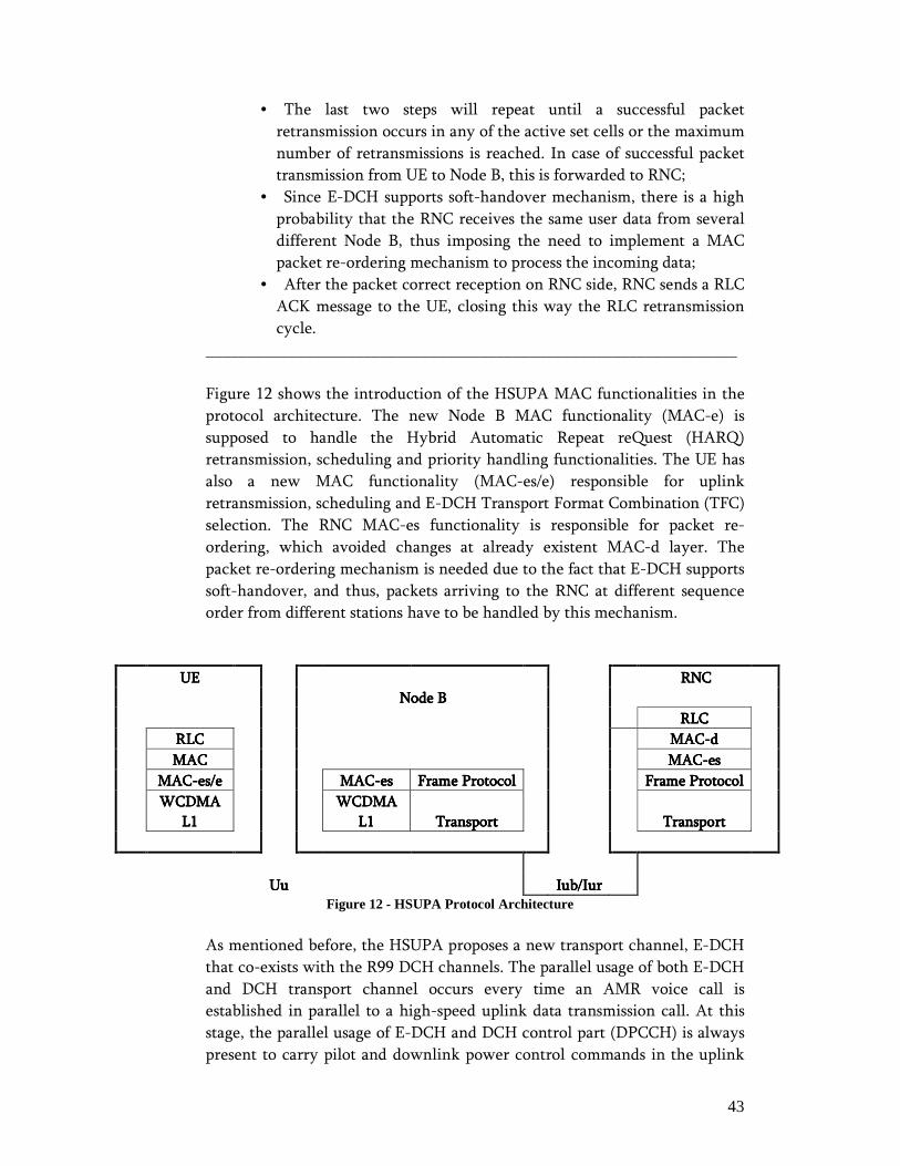
Figure 12 shows the introduction of the HSUPA MAC functionalities in the
protocol architecture. The new Node B MAC functionality (MAC-e) is
supposed to handle the Hybrid Automatic Repeat reQuest (HARQ)
retransmission, scheduling and priority handling functionalities. The UE has
also a new MAC functionality (MAC-es/e) responsible for uplink
retransmission, scheduling and E-DCH Transport Format Combination (TFC)
selection. The RNC MAC-es functionality is responsible for packet re-
ordering, which avoided changes at already existent MAC-d layer. The
packet re-ordering mechanism is needed due to the fact that E-DCH supports
soft-handover, and thus, packets arriving to the RNC at different sequence
order from different stations have to be handled by this mechanism.
UEUEUEUE RNCRNCRNCRNC
Node BNode BNode BNode B
RLCRLCRLCRLC
RRRRLCLCLCLC MACMACMACMAC----dddd
MACMACMACMAC MACMACMACMAC----eseseses
MACMACMACMAC----es/ees/ees/ees/e MACMACMACMAC----eseseses Frame ProtocolFrame ProtocolFrame ProtocolFrame Protocol Frame ProtocolFrame ProtocolFrame ProtocolFrame Protocol
WCDMA WCDMA WCDMA WCDMA
L1L1L1L1
WCDMA WCDMA WCDMA WCDMA
L1L1L1L1 TransportTransportTransportTransport TransportTransportTransportTransport
UuUuUuUu Iub/IurIub/IurIub/IurIub/Iur Figure 12 - HSUPA Protocol Architecture
As mentioned before, the HSUPA proposes a new transport channel, E-DCH
that co-exists with the R99 DCH channels. The parallel usage of both E-DCH
and DCH transport channel occurs every time an AMR voice call is
established in parallel to a high-speed uplink data transmission call. At this
stage, the parallel usage of E-DCH and DCH control part (DPCCH) is always
present to carry pilot and downlink power control commands in the uplink
44
direction. The E-DCH introduction has impacts on the physical layer
architecture with the introduction of several UL and DL channels.
The channels introduced in UL are:
• Enhanced Dedicated Physical Data Channel (E-DPDCH) – this
physical channel maps the E-DCH transport channel for user data
transmission on radio interface;
• Enhanced Dedicated Physical Control Channel (E-DPCCH) – this
is the control channel that provides feedback to the Node B about
the data sent through E-DPDCH.
The DL channels are:
• Absolute Grant Channel (E-AGCH) – provides information to UE
about the transmission power level that must be adopted in the
next TTI. The E-DCH power level must always be higher than the
DPDCH (physical channel associated with DCH) power level;
• Relative Grant Channel (E-EGCH) – indicates the UE to whether
increase, decrease or maintains its E-DCH transmission power.
• HARQ Acknowledgement Indicator Channel (E-HICH) – channel
used by Node B to provide feedback to UE about the HARQ
Acknowledge/Non-Acknowledge messages.
The main differences between Rel99 DPDCH and E-DPDCH are:
• Rel99 DPDCH may use 10, 20 or 40 ms TTI, while E-DPDCH may
use 10 or 2 ms TTI. The possibility of using a 2 ms TTI contributes
for decreasing the round-trip time, but can result in excessive
control information exchange if UE is on the cell edge;
• While in the early HSUPA releases the modulation is unchanged
when compared with Rel99 modulation scheme (BPSK), the
release 7 introduces the possibility of using 16QAM, which also
allows to support even higher data rates, in UL, when good radio
conditions occur;
• In the earlier HSUPA releases, since the modulation scheme
remains unchanged, the increase in UL data rates is achieved with
the extensive use of multi-code transmission. The Rel99 practical
usage scenario is of a single SF4 code in UL transmission, which
results in a peak user data rate of 384 kbps. In the E-DPDCH case,
the data rates are a result of multi-code combination and the
introduction of SF2. The combination of two SF4 channels with
another additional two SF2 channels provide the ability to reach
the maximum physical layer bit rate of 5.76 Mbps;
• E-DPDCH is responsible for carrying user data only and relies
upon DPCCH to carry UE feedback about pilot quality, and on E-

45
DPCCH to carry the HSUPA-related physical layer control
information.
E-DPCCH carries in a single message three different types of information:
• 7 bits for E-DPDCH-related rate information;
• 2 bits for retransmission related information that can either
indicate that it is a new packet transmission or a retransmission of
previously sent packet. In the case of a retransmission, the
transmission redundancy version is also indicated;
• 1 bit that informs the Node B about the UE need to increase the
corresponding data rate. This is implemented in a form of a Happy
Bit, if the bit is set to “happy” state this means that the UE is
satisfied with the current bit rate that is being served, and thus
there is no need for the scheduler to increase it.
These are the most important physical channels due to the fact that they are
directly responsible to implement E-DCH and its innovations.
The HSUPA Node B scheduler operation details can be described as follows:
• The Node B scheduler senses the medium and takes measurements
of its condition, for instance the noise level (interference at the
Uplink) to decide if there is capacity to allocate more traffic to a
specific cell, or to decide if current user’s data rate must be lowered
to decrease uplink interference;
• The scheduler also monitors the received UE specific feedback, the
Happy Bits, taking into knowledge what are the users that could
transmit at a higher data rate. It also relates the happy bit
information against its own MAC-e buffer availability and uplink
power headroom availability, which allows the scheduler to decide
if there is available capacity to increase the data rate for each user
requesting higher throughput;
• The scheduler makes also use of defined user priority configured at
the RNC, to decide what should be the data rate adjustment to be
applied to a specific user or set of users. It can be the case that
there is the request from a specific user to increase the data rate
(Happy Bit set as “unhappy”) and the available capacity to provide
it, but the user priority handling configuration does not allow such
upgrade.
This mode of operation implies that the RNC instructs the Node B what is the
maximum data rate allowed for a specific service subscription/user profile. For
the same subscriber there can be different priorities depending on the type of
service that is being accessed. This is done making use of MAC flow identifiers.
46
It should be noted that there are traffic types that do not make use of scheduled
transmission. This is the case of Signaling Radio Bearer (SRB) related information
or, for instance, VoIP service. Both of types of data require a very limited delay
or jitter value and lower throughput, which means that scheduling this kind of
data would just imply a degradation of service delivery, for instance due to UE
delayed measurement reports. For this kind of services, the RNC provides
permanent grant that the Node B scheduler cannot change. Thus, the non-
scheduled transmission operates like R99 DCH (not using Node B scheduler
capabilities), with the significant difference that it still takes advantage of the
Fast L1 HARQ mechanism.
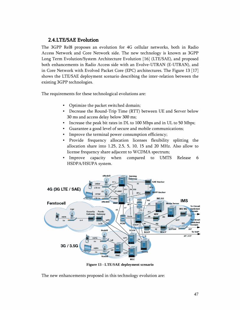
47
2222....4444.... LTELTELTELTE/SAE/SAE/SAE/SAE Evolution Evolution Evolution Evolution
The 3GPP Rel8 proposes an evolution for 4G cellular networks, both in Radio
Access Network and Core Network side. The new technology is known as 3GPP
Long Term Evolution/System Architecture Evolution [16] (LTE/SAE), and proposed
both enhancements in Radio Access side with an Evolve-UTRAN (E-UTRAN), and
in Core Network with Evolved Packet Core (EPC) architectures. The Figure 13 [17]
shows the LTE/SAE deployment scenario describing the inter-relation between the
existing 3GPP technologies.
The requirements for these technological evolutions are:
• Optimize the packet switched domain;
• Decrease the Round-Trip Time (RTT) between UE and Server below
30 ms and access delay below 300 ms;
• Increase the peak bit rates in DL to 100 Mbps and in UL to 50 Mbps;
• Guarantee a good level of secure and mobile communications;
• Improve the terminal power consumption efficiency;
• Provide frequency allocation licenses flexibility splitting the
allocation share into 1.25, 2.5, 5, 10, 15 and 20 MHz. Also allow to
license frequency share adjacent to WCDMA spectrum;
• Improve capacity when compared to UMTS Release 6
HSDPA/HSUPA system.
Figure 13 - LTE/SAE deployment scenario
The new enhancements proposed in this technology evolution are:

48
• Use of Orthogonal Frequency Division Multiple Access (OFDMA) and
advanced multiple antenna techniques over the air-interface;
• Distributed (as opposed to centralized) architecture for RAN;
• IP-based Radio and Core Network;
The OFDMA together with multiple antenna techniques increase significantly the
spectral efficiency, while OFDM is highly scalable. Therefore, going from 1.25 MHz
or 5 MHz to a 20MHz channel bandwidth is achievable, thus offering higher peak
data rates. This efficient air-interface allows many users to experience data rate in
excess of 1Mbps, being the peak data rate target 100 Mbps in a 20MHz spectrum in
downlink. The 3GPP access is based on OFDMA in downlink direction and Single
Carrier-Frequency Division Multiple Access (SC-FDMA) in uplink.
A distributable RAN architecture allows reduced latency, since most dynamic
decisions are made locally in the evolved-Node B (e-Node B). Since the Radio
Resource Management decisions are taken close to the air-interface and the UE,
therefore the required QoS parameters of a multimedia application can be managed
is a more efficient manner. The proposed IP-based RAN results in an easy-to-scale
network.
A fully packetized IP-based CN will replaced 3G CS and PS networks, providing
high scalability and reduce cost. It also simplifies the introduction of new services
via the IP Multimedia Subsystem (IMS). A very important feature introduced by the
IP-based architecture is the capability to implement seamless mobility between
different RAN technologies without impacting the session logical layer, which is
managed by Mobile IP protocol. This enables the ability, in handover control, to
always select the RAN from session level perspective.
LTE/SAELTE/SAELTE/SAELTE/SAE Architecture Architecture Architecture Architecture
The 3GPP LTE places the full radio functionality in the base station, so Evolved
UTRAN (E-UTRAN) architecture consists of an evolved Node B (eNodeB). The
interface between the eNodeBs is known by X2, which provides the means to
support handovers. Figure 14 introduces a LTE architecture overview representing
all the network elements and interfaces.

49
S1
S1
S1
S1
X2
X2
Figure 14 - LTE Architecture
The eNodeB new functionalities, when compared with HSDPA/HSUPA Node B, are
RLC, RRC and PDCP layers.
Figure 15 - LTE/SAE Protocol Architecture
From Figure 15 it can be depicted that the eNodeB connects to the new core
network via a S1 interface, where S1 can have two distinct implementations in the
core side: S1-MME and S1-U. The S1-MME connects eNodeB to the Mobility
Management Entity (MME) and the S1-U to the Serving SAE Gateway (SGW) and
Public Data Network SAE Gateway (PGW). The MME is the element responsible for
handling the control plane signaling, specially the mobility management and idle-
mode handling. In other hand, the SGW and PGW are responsible for processing
the user plane data, as for mobility management inside LTE and between 3GPP
RATs. In the new SAE core architecture, the interface that connects MME and
SGW/PGW is S11 interface. There are two additional elements on the core side,
Home Subscriber Server (HSS) and Policy and Charging Rules Function (PCRF). HSS
covers the functionalities that HLR has for both 2G and 3G networks, and contains

50
user specific information on service priorities, data rates, etc. The PCRF is related
with the appliance of QoS and Charging policies.
This new flat network all-IP architecture provides high data rates, is scalable for
increasing data volumes and adds capacity to support the increasing number of users,
which in turn enables its cost efficiency.
LTE/SAE Performance MonitoringLTE/SAE Performance MonitoringLTE/SAE Performance MonitoringLTE/SAE Performance Monitoring
The new flat All-IP architecture introduced by LTE and SAE advantages are not
only related with network capability enhancements, but it brings also great and new
things for the Performance Management field. The simplified user plane protocol
stack, the evolution towards IP transmission links and the IP End-to-End native
network brings new light to Service QoS performance and Network performance
relation. Much of the IP-based Service metrics defined in this work, that in 3G are
spread around a multitude of data sources, will be available on LTE/SAE as simple
PM data which simplifies the access to this information.
Therefore, this means that this thesis work proposal is very much aligned with the
innovation trend, and it can be also envisioned that, with few adjustments, it can be
extended and simplified for the LTE/SAE support.
51
2222....5555.... SummarySummarySummarySummary
This chapter introduced the Network Management thematic describing some of
the most used performance monitoring techniques and introducing the
Telecommunications Management Network (TMN) Model that was used as the
basis concept for this work. TMN Model proposes a layered network
management approach, detailing the following layers: Business Management
Layer (BML), Service Management Layer (SML), Network Management Layer
(NML), Element Management Layer (EML) and Network Element Layer (NEL).
This chapter also introduced the Packet Switched Network architecture, its
network elements and functional parts: UTRAN and CN. The UTRAN is
composed by the following elements and interfaces: RNC, Node B, UE, Iur, Iub
and Uu. While the CN part is composed by SGSN, GGSN and Iu, it also details
with the packet session establishment procedure as it is crucial for this work to
understand the signaling process behind UMTS network access.
An important part of this chapter is dedicated to describe the UMTS Radio
Access Technologies that enable the capability to transmit efficiently real-time
multimedia user data. This chapter compares the UMTS R99 features with the
HSDPA and HSUPA key features, highlighting this way the reasons for this
3GPP evolution path and how higher bit rates, less delay and latency, just to
name few indicators, are achieved. HSDPA and HSUPA make use of techniques
like: L1 Hybrid ARQ Fast Retransmission, Multi-Coding, Adaptive Modulation
and Coding and Node B MAC Scheduling.
The last section of this chapter introduced the new 3GPP technological proposals:
UMTS Long Term Evolution (LTE) and Service Architecture Evolution (SAE).
These proposals main objective is to cope with 4G network requirements and the
key are: Flat Architecture with less elements in the data path, thus reducing the
latency; OFDMA, multi-antenna and scalable bandwidth allow a more efficient
air-interface increasing the capacity and improving user experience; All-IP
architecture simplifies the User Plane protocol stack and enables key features
like seamless mobility between different RAN technologies, using for this the
Mobile IP protocol.

52
3333.... Performance ManagementPerformance ManagementPerformance ManagementPerformance Management
Performance statistics play a central role in all network operational,
maintenance, troubleshooting, planning and optimization procedures. Each
performance statistic is fairly unique and is always related with a specific
network parameter or event. There are many parameters, protocols and events
that can be monitored, and thus, there are many related statistics that can be
related between each other, which leaves to an infinite number of possible
permutations. In this highly complex scenario, the challenge is to identify which
are the most relevant statistics that must be monitored and analyzed in case of a
particular network failure. This is the challenge that Performance Management
Systems try to address.
This chapter is divided in six sections. Section 3.1 provides detailed description
of the proposed Performance Management Architecture proposed by this work,
and also details the fundamental elements and their functionality and purpose.
Section 3.2 describes in detail all the performance management data sources both
for network and IP-based service layer. The Section 3.3 introduces the ETL
process as part of Performance Management cycle. Section 3.4 presents the
network and IP-based service object model detailing the database structure for
PM data storage. Section 3.5 provides a detailed description about the proposed
KPIs included in this work. The last section, 3.6, describes the proposed
reporting use case, which combines network and service statistical data.
3333....1111.... Architecture OverviewArchitecture OverviewArchitecture OverviewArchitecture Overview
This highly demanding network scenario requires a high performance, well
organized, optimized and comprehensive PM system that can be used to assist
network operator to take accurate actions in the least time possible. Figure 16
shows the proposed Performance Management system architecture, providing a
complete overview from performance statistics sources to the mediations,
adaptations, data storage and reporting applications.
Figure 16 - Performance Management: System Architecture
53
Performance Management ConceptPerformance Management ConceptPerformance Management ConceptPerformance Management Conceptssss
There are two conceptual elements that are transversal to the PM System
Architecture: Performance Measurement and Performance Counter. A third
important conceptual element that can be derived from those elements is the
Key Performance Indicator.
Network ElementsNetwork ElementsNetwork ElementsNetwork Elements
Each network element monitors its performance through the Performance
Mediation. A subset of that module is responsible for the communication with
the Element Manager. That interface is divided into three types of primitives
relating to the type of data which is to be transported; Performance Management
data (PM), Configuration Management data (CM) and Fault Management Data
(FM). The first is intended to present metrics related with the continuous
operation of the equipment, while the second indicates the configuration setup,
including information such as topology and capabilities. FM is a more urgent
type of data as it indicates critical issues to be evaluated. In figure 15 it is only
present NodeB and RNCs, but any type of network nodes could be included
beyond the Radio Network System (RNS).
Element managerElement managerElement managerElement manager
The NE Mediation manages the interactions between the Element Manager
Module and the several Network Elements in the network. It is responsible for
the collection of the Performance and Fault Management functions existing in
each of the elements of the network. The NE Mediation Module implements the
Extraction part of an ETL procedure.
The statistics Processor is responsible for converting all the diverse data gathered
from the NEs according to a structured and generic meta-model, which will be
briefly discussed ahead. This particular module processes Configuration,
Performance and Failure Management Information.
The Raw Database loader is responsible for providing interfaces for the access
relating to data storage management features. It is another function of an ETL
procedure the upload of the gathered information into the raw databases. This
module includes interfaces for mediation of the interactions between the EM
and the analysis tools that evaluate the collected data. These interfaces answer to
the Reporting Tool for requests related to CM, PM and FM data.
Reporting ToolReporting ToolReporting ToolReporting Tool
Reporter Database is a data warehouse designed for the coherent integration of
diverse data sources, dimensioned to optimize the data discovery and reporting.
This data repository modulates all the network topology into a hierarchal object
structure, which provides the capability to analyze the entire network. This
analysis can focus on the correlation of different parameters that can be
Configuration, Performance or Fault Management related. A possible use case
would be to assess what kind of configuration optimizes better the performance
54
of the network, by improving network capacity and reducing its faults. This
analysis can be extended in time and from different network perspectives, as
historical and object data aggregation is possible. Moreover, the database
primitives allow for the storage management and provide all the data access
information to other layers.
This database is modulated based on NE specific metadata, which defines the
Object Class (OC) structure, and for each OC all the PM Measurements, and
related list of PM Counters and aggregation rules. The FM metadata is generic
for all the OC, defining a list of failures that can occur.
Statistics Post-Processor is a software component that plays a decisive part on the
reporting process. It is responsible for the entire object and time aggregations,
which enhances the analysis capabilities, allowing the time trend analysis and
drilling through the network objects, allowing a great diversity of network
analysis. The aggregation rules are all defined through metadata specific for each
NE, and provide information on how PM counters must be aggregated in time or
in OC dimensions. For instance, these rules can define that a specific counter
that is collecting information about the failed allocations of a specific cell
resource, must be summed in time domain and in object domain, which results
that this counter is counting, for the original object level, sequentially in time all
the failure events, and when aggregated to a greater order object (Node B for
instance), will accumulate all the contribution of the related cells.
Reporting Engine is the mind behind Reporter Tool. It is responsible for the
database queries, it processes the results and displays them in a defined format. It
provides all the data visualization capabilities, offering different pre-defined
models and allowing the user to create their own. These pre-defined
visualization models are important, because they allow the manipulation of data
in different dimensions and the drilling through them, providing this way,
different reports for different types of end users and even for different type of
analysis, starting from a unique data set. Related to these models, there is an
important reporting component, this is the Key Performance Indicators (KPI) set.
A KPI is a data aggregation that provides fundamental information for the
understanding of network behavior. It can be as simple as selecting a particular
important counter, or as complex as implementing an arithmetic calculus,
enhancing this way the data visualization capabilities. KPIs are defined in
configuration components and can be either calculated on the fly by reporting
engine or pre-calculated and store in Reporter Database.
The Automated Knowledge Discovery model is another important part of this
reporting engine and provides the very important feature of automatic data
monitoring, searching for patterns in the network behavior for the sake of
forecasting upcoming events, such as Operation & Maintenance and
Optimization needs.

55
3333....2222.... MetadataMetadataMetadataMetadata
The metadata describes all the elements that are part of the information model,
from the modeled network elements and its functional parts, to the performance
measurement and counters. Every technology must have a set of metadata
information that describes all the relations between all the monitored NEs,
protocols, procedures and resources. Metadata is divided into three logical parts:
Configuration Management (CM), Performance Management (PM) and Fault
Management (FM).
3333....2222....1111.... Configuration Management (CM)Configuration Management (CM)Configuration Management (CM)Configuration Management (CM)
Configuration Management metadata is responsible for the mapping
between the different NE present in the network and their components
into a coherent and structured Object Class model. This way, CM
metadata is used to identify objects with the same properties and to
maintain possible occurrences of an object in the object class hierarchy.
Two types of objects can de defined for this model, Managed Objects (MO)
and Reference Objects (RO). Managed Objects refer to objects that are
directly related elements present in the network that can be managed,
configured, manipulated, which are obviously the NE elements and their
components e.g. a Node B and its Cells. Reference Objects refer to virtual
reporting dimensions, i.e. elements that are virtually created to ease the
network analysis by dividing and grouping the network into smaller
segments thus reducing the analysis complexity. This Reference Objects
are created and stored in to the Reporter Database by the Statistics Post-
Processor module, using the CM metadata info.
Managed Objects have the foManaged Objects have the foManaged Objects have the foManaged Objects have the following data structure:llowing data structure:llowing data structure:llowing data structure:
• MOC ID – the numerical object class ID, that unequivocally identifies
the Object Class within the object tree;
• MOC Vendor – identifies the vendor of the network resource;
• MOC Version – identifies the network resource version;
• OC Name – object class name that is displayed in the Reporter
application, e.g. “NodeB”;
• MOC Abbreviation – abbreviation used for the OC, for example “NB”;
• MOC Time Stamp – the time when MO was last modified in the
Reporter Database;
• MOC Description – description of the object class and the network
resource that it maps;
• MOC Parent ID – the numerical number OC ID of the parent object
class, if applicable. In case the OC is the root object class, this field is filled
by default with the value “1”.
Reference ObjecReference ObjecReference ObjecReference Objects have the following data structure:ts have the following data structure:ts have the following data structure:ts have the following data structure:
56
• ROC ID – – the numerical object class ID, that unequivocally identifies
the Object Class within the object tree;
• ROC Name – object class name that is displayed in the Reporter
application, e.g. “Local Cell Group”;
• ROC Abbreviation – abbreviation used for the OC, for example “LCG”;
• ROC Time Stamp – the time when MO was last modified in the
Reporter Database;
• ROC Description – description of the object class and the network
resource that it maps;
• ROC Reference ID – since the Reference Object is always associated to
one or more MOC instance, this field is used to store each object ID that is
related to this reference object. For the LCG example, ROC Reference ID
should be equal to each Cell MOC ID related that is part of it.
3333....2222....2222.... Performance Management (PM)Performance Management (PM)Performance Management (PM)Performance Management (PM)
Performance Measurement Metadata is responsible for defining, for each
network element, all the PM measurements and Counters and relating
them to the CM data, i.e. to the OC structure. As network element
represents a specific role in the network, there will be a different set of
measurements/counters for each NE. The number of measurements and
counters needed to monitor a specific NE is dependent on the NE
complexity, ranging with the number of functionalities. A PM
measurement is a logic representation of a NE functionality that defines a
set of counters that monitors the network performance behavior. A PM
Counter is the fundamental element of the performance monitoring
process, as it provides detailed information ranging from specific
procedures until group functions. As Counters are the basis of PM, from
its values and monitoring purposes, there can be developed different
kinds of aggregations such as KPIs and Reports, that allows to level the
analysis from the most detailed information where there can be
thousands of counters, through hundreds of KPIs and tens of reports for
each object class, and ending with only one overview report containing
only the most abstract and descriptive data. This way, different kinds of
users and analysis can be satisfied with only one tool.
3333....2222....3333.... Fault Management (FM)Fault Management (FM)Fault Management (FM)Fault Management (FM)
Fault Management Metadata defines the mapping between all the NE
components and the fault events that describe system failures that can be
either hardware or software driven. FM metadata thus relates OC with
incoming network failure notifications. These failures are categorized and
ranked by severity, which can range from debug to emergency state.
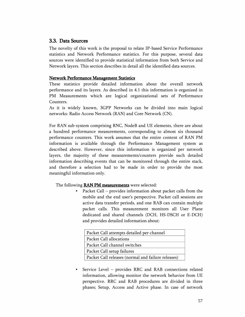
57
3333....3333.... Data SourcesData SourcesData SourcesData Sources
The novelty of this work is the proposal to relate IP-based Service Performance
statistics and Network Performance statistics. For this purpose, several data
sources were identified to provide statistical information from both Service and
Network layers. This section describes in detail all the identified data sources.
Network PerNetwork PerNetwork PerNetwork Performance Management Statisticsformance Management Statisticsformance Management Statisticsformance Management Statistics
These statistics provide detailed information about the overall network
performance and its layers. As described in 4.1 this information is organized in
PM Measurements which are logical organizational sets of Performance
Counters.
As it is widely known, 3GPP Networks can be divided into main logical
networks: Radio Access Network (RAN) and Core Network (CN).
For RAN sub-system comprising RNC, NodeB and UE elements, there are about
a hundred performance measurements, corresponding to almost six thousand
performance counters. This work assumes that the entire content of RAN PM
information is available through the Performance Management system as
described above. However, since this information is organized per network
layers, the majority of these measurements/counters provide such detailed
information describing events that can be monitored through the entire stack,
and therefore a selection had to be made in order to provide the most
meaningful information only.
The following RAN PM measurementsRAN PM measurementsRAN PM measurementsRAN PM measurements were selected:
• Packet Call – provides information about packet calls from the
mobile and the end user’s perspective. Packet call sessions are
active data transfer periods, and one RAB can contain multiple
packet calls. This measurement monitors all User Plane
dedicated and shared channels (DCH, HS-DSCH or E-DCH)
and provides detailed information about:
Packet Call attempts detailed per channel
Packet Call allocations
Packet Call channel switches
Packet Call setup failures
Packet Call releases (normal and failure releases)
• Service Level – provides RRC and RAB connections related
information, allowing monitor the network behavior from UE
perspective. RRC and RAB procedures are divided in three
phases; Setup, Access and Active phase. In case of network
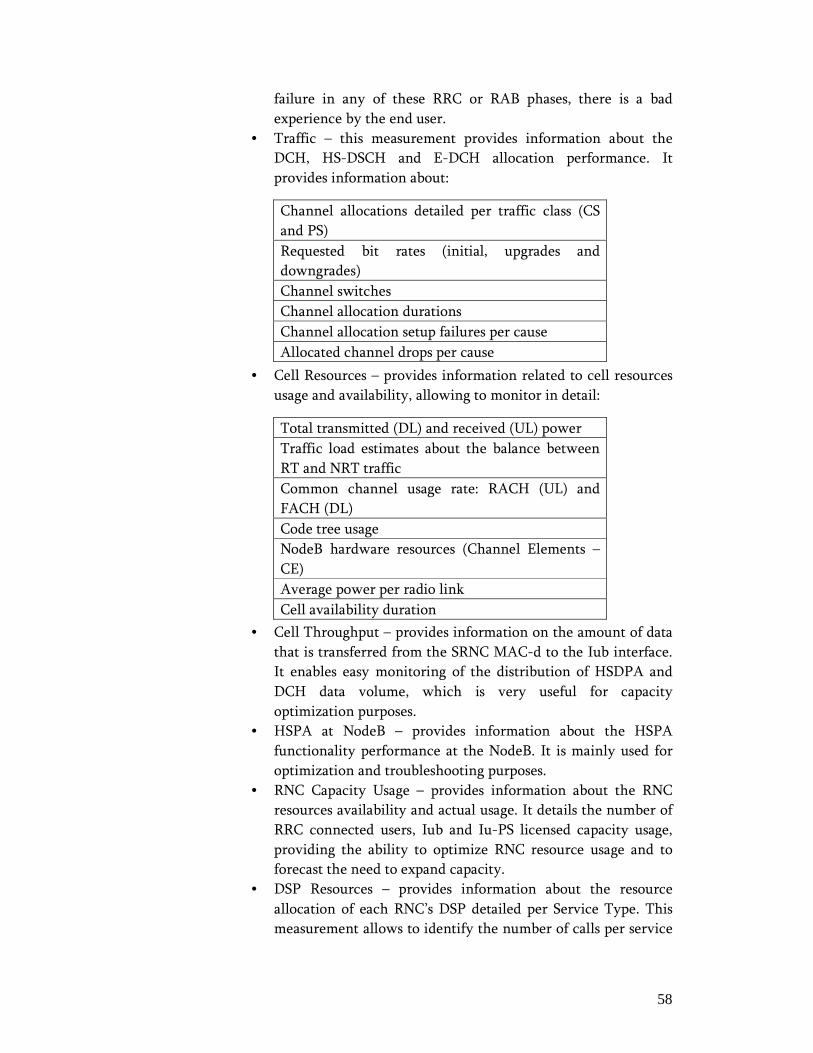
58
failure in any of these RRC or RAB phases, there is a bad
experience by the end user.
• Traffic – this measurement provides information about the
DCH, HS-DSCH and E-DCH allocation performance. It
provides information about:
• Cell Resources – provides information related to cell resources
usage and availability, allowing to monitor in detail:
• Cell Throughput – provides information on the amount of data
that is transferred from the SRNC MAC-d to the Iub interface.
It enables easy monitoring of the distribution of HSDPA and
DCH data volume, which is very useful for capacity
optimization purposes.
• HSPA at NodeB – provides information about the HSPA
functionality performance at the NodeB. It is mainly used for
optimization and troubleshooting purposes.
• RNC Capacity Usage – provides information about the RNC
resources availability and actual usage. It details the number of
RRC connected users, Iub and Iu-PS licensed capacity usage,
providing the ability to optimize RNC resource usage and to
forecast the need to expand capacity.
• DSP Resources – provides information about the resource
allocation of each RNC’s DSP detailed per Service Type. This
measurement allows to identify the number of calls per service
Channel allocations detailed per traffic class (CS
and PS)
Requested bit rates (initial, upgrades and
downgrades)
Channel switches
Channel allocation durations
Channel allocation setup failures per cause
Allocated channel drops per cause
Total transmitted (DL) and received (UL) power
Traffic load estimates about the balance between
RT and NRT traffic
Common channel usage rate: RACH (UL) and
FACH (DL)
Code tree usage
NodeB hardware resources (Channel Elements –
CE)
Average power per radio link
Cell availability duration

59
type (HSDPA, HSUPA, CS Voice, CS Video, etc.), which is
important to evaluate the network traffic model.
• Iu-PS Performance – provides statistical information about the
Iu-PS traffic load and GTP-U (GGSN Tunneling Protocol –
User Plane) throughput between RNC and PS Core.
• RCPM RLC – provides information about the performance of
user data transfer on RLC layer, for connection types that uses
Acknowledge Mode (AM RLC), which are:
The scope of RCPM RLC measurement can be seen in the
following figure:
Figure 17 - Scope of RCPM RLC Measurement
As it can be depicted from Figure 17, this is a very important
measurement, since it provides information about RLC UP data
delivery performance that can be directly related with the Iu-
PS throughput.
For CN sub-subsystem, it is only considered the Packet Switched part, which is
composed by two major NEs: Serving GPRS Support Node (SGSN) and Gateway
GPRS Support Node (GGSN). Since these nodes functionalities are very different
and complementary between them, a separate analysis for each of these nodes is
required.
Signaling Radio Bearers
PS NRT (PS Background and PS Interactive) user
data connections, which includes HSDPA and
HSUPA
PS RT (PS Streaming) user data connections,
which also includes HSDPA and HSUPA
connections
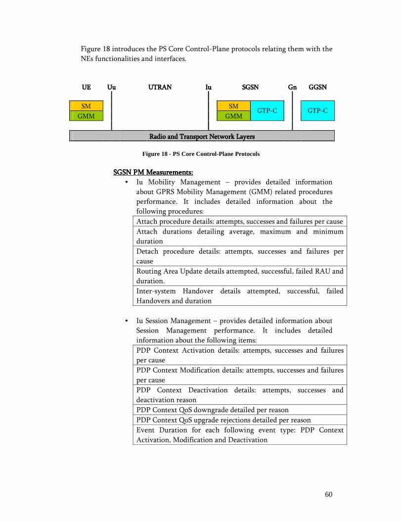
60
Figure 18 introduces the PS Core Control-Plane protocols relating them with the
NEs functionalities and interfaces.
UEUEUEUE UuUuUuUu UTRANUTRANUTRANUTRAN IuIuIuIu SGSNSGSNSGSNSGSN GnGnGnGn GGSNGGSNGGSNGGSN
SM SM
GMM GMM GTP-C
GTP-C
Radio and Transport NetworkRadio and Transport NetworkRadio and Transport NetworkRadio and Transport Network Layers Layers Layers Layers
Figure 18 - PS Core Control-Plane Protocols
SGSN PM Measurements:SGSN PM Measurements:SGSN PM Measurements:SGSN PM Measurements:
• Iu Mobility Management – provides detailed information
about GPRS Mobility Management (GMM) related procedures
performance. It includes detailed information about the
following procedures:
Attach procedure details: attempts, successes and failures per cause
Attach durations detailing average, maximum and minimum
duration
Detach procedure details: attempts, successes and failures per
cause
Routing Area Update details attempted, successful, failed RAU and
duration.
Inter-system Handover details attempted, successful, failed
Handovers and duration
• Iu Session Management – provides detailed information about
Session Management performance. It includes detailed
information about the following items:
PDP Context Activation details: attempts, successes and failures
per cause
PDP Context Modification details: attempts, successes and failures
per cause
PDP Context Deactivation details: attempts, successes and
deactivation reason
PDP Context QoS downgrade detailed per reason
PDP Context QoS upgrade rejections detailed per reason
Event Duration for each following event type: PDP Context
Activation, Modification and Deactivation

61
• Iu Data Measurement – provides detailed information about
the amount of data transmitted through Iu interface. It
includes the following details:
Both GTP-U DL (SGSN –> RNC) and UL (RNC -> SGSN)
throughputs, sent packets and amount of dropped data
Both GTP-U DL and UL throughputs, sent packets and amount of
dropped data, detailed per associated priority queues
Both DL and UL throughputs, sent packets and amount of dropped
data, detailed per traffic class, bearer class
DL and UL transmitted data detailed per PDP context providing
the average throughput per PDP and the peak value occurrence
• User Management Measurement – provides detailed
information about the User status. It includes the following
details:
Attached Users details: average and peak number of attached users
Access Control details: the denied access requests per reason
PDP Contexts: details the average and peak number of active PDP
contexts per priority classes. It also provides PDP activation
rejections details
Active Subscribers: details the average and peak number of
subscriber with active PDP Contexts
• CDR Measurement – provides detailed information about Call
Detail Records controlled in SGSN. It provides the following
details:
CDR generation: provides the number of generated CDR per
subscriber type and the number of discarded CDR per reason
CDR duration: details the open CDRs average duration
• Iu RANAP Measurement – provides detailed and important
information about the signaling changed between RAN and
CN:
RAB Events: details the number of attempted, released and failed
RAB establishments. It also details the RAB establishment failures
per cause
Active RAB: details the average and peak number of active RABs
GGSN PM Measurements:GGSN PM Measurements:GGSN PM Measurements:GGSN PM Measurements:
• General Indicators – provides detailed information about
Packet Switched load metrics measured at dedicated data
processors. It provides the following statistics:
CPU load due to Packet Switching: details the average and

62
maximum values
Total Throughput: details the average and maximum throughput
value for the entire GTP set. Throughput values can be of Packet
per second and Mbit per second
Packet Size: details the average and maximum packet size in bytes
Erroneous GTP packets: details the number of erroneous packet for
both DL (GGSN to SGSN) and UL (SGSN to GGSN) traffic
directions
• Session Management – provide detailed information about
PDP Context. It provides the following statistics:
PDP Context Events: details the amount of, PDP create, update
and delete messages received from SGSN. It also details each of
these events per cause code
Active PDP Context: details the amount current active PDP
Contexts. It also details the average and peak number of active
PDP Context
PDP Context Duration: details the average and maximum active
PDP context duration
Dynamic IP Address Usage: details the current number of
allocated dynamic IP addresses. It also provides the average,
maximum number and usage rate of dynamic IP addresses
• GTP Data per Access Point Network (APN) – provides detailed
information about GTP transmitted data related with a specific
APN. It provides the following statistics:
GTP Packets: details the number of sent and received packets
during the period duration
GTP Data: details the sent and received data volume of during the
period duration
GTP Error Free Bytes: details the sent and received error free data
volume during the period duration
• Traffic QoS at GGSN Level – provides detailed information
about transmitted traffic, detailed per QoS traffic class. It
provides the following statistics:
Throughput: details the DL and UL throughput per QoS traffic
class
DL Dropped Data: details the amount of dropped data in DL
direction, detailed per QoS traffic class
Active PDP Contexts: details the number of active PDP Contexts
per QoS traffic Class
Rejected PDP Context: details the number of rejected PDP
63
Context activation requests per QoS traffic Class, due to lack of
resources
• Traffic QoS at APN Level – provides detailed information
about transmitted traffic, related with a specific APN, detailed
per QoS traffic class. It provides the following statistics:
Throughput: details the DL and UL throughput per QoS traffic
class
DL Dropped Data: details the amount of dropped data in DL
direction, detailed per QoS traffic class
• Service Specific – provides detailed information about
transmitted traffic, related with a specific service (HTTP, WAP,
FTP, P2P, etc.). It provides the following statistics:
Throughput: details the DL and UL throughput per Service
Dropped Data due to limited Bandwidth: details the amount of
dropped data per Service
Call Detail RecordCall Detail RecordCall Detail RecordCall Detail Record
Call Detail Record is a file generated by the system for every call that is
established and describes detailed billing information. Although originally the
CDR was designed to describe call details for billing purposes, its information
can be used to trace the call at the business level and retrieve service assurance
relevant information.
This information complements the Performance Management information by
extending the network behavior analysis to the service/subscriber scope,
providing the ability to propose new analysis scenarios, e.g. to assess if network
is accurate in the service delivery or which services are more suitable for that
network considering its traffic model and user behavior.
The following fields were identified as being important from service
assurance point-of-view:
• recordOpeningTimerecordOpeningTimerecordOpeningTimerecordOpeningTime – this field provides information about the time
when the CDR was created and thus the session creation time.
• changeTimechangeTimechangeTimechangeTime – the time when this record was closed and therefore the
session ended.
• accessPointNameaccessPointNameaccessPointNameaccessPointName – this field indicates the type of external Packet Data
Network (PDN) that was accessed by user during the session period.
• ggsnAddressggsnAddressggsnAddressggsnAddress – this field provides the control plane IP address of the
serving GGSN.
64
• sessionIdsessionIdsessionIdsessionId – this field provides the PDP context session identifier.
Together with the ggsnAddressggsnAddressggsnAddressggsnAddress and userLocationInformationuserLocationInformationuserLocationInformationuserLocationInformation, it allows to
identify the complete network data path.
• servedIservedIservedIservedIMSI MSI MSI MSI – this field provides International Mobile Subscriber Identity
(IMSI) of the served party, the user.
• servedPDPAddressservedPDPAddressservedPDPAddressservedPDPAddress – this field provides the IP address related with the
PDP context activated for the served IMSI.
• accessTypeaccessTypeaccessTypeaccessType – this field indicates which is the Radio Access Network type
that served the connection in RAN side. This field can assume the
following values:
o 1 (GTP_RAT_TYPE_UTRAN): 3G (UMTS) RAN;
o 2 (GTP_RAT_TYPE_GERAN): 2G (GSM(GPRS) / EDGE)
RAN;
o 3 (GTP_RAT_TYPE_WLAN): WLAN.
• userLocationInforuserLocationInforuserLocationInforuserLocationInformationmationmationmation – this field provides information about the end
user location during the all CDR life cycle. The location information
consists of the following parts:
o geographic location area
o location area code (LAC)
o cell identity (CI) /service area code (SAC)
DeepDeepDeepDeep Packet Inspection Packet Inspection Packet Inspection Packet Inspection
“Deep Packet Inspection” (DPI) is a computer networking term that refers to
devices and technologies that inspect and take actions based on the contents of
the packet (commonly called the “payload”) rather than just the packet header.”
[18]
Deep Packet Inspection can be used for a wide range of applications and a
common use can be described by an inspection point where packets pass and are
inspected in order to search for protocol non-compliances, viruses, spam and
intrusions. Although DPI wide spread use is related to security applications, it
allows pre-configurations of analysis criteria in order to decide what actions to
take on the packet. This can be used to extend its capabilities for other purposes,
rather than security, like statistical collection. From this work perspective, the
ability to collect IP based protocol statistics is the most relevant DPI
functionality. It will enhance the service/session performance monitoring
capabilities by providing means of collecting information about SIP, RTP and
other protocols that can be considered relevant depending on the IP service that
is under analysis scope.
Session Initiation Protocol (SIP)Session Initiation Protocol (SIP)Session Initiation Protocol (SIP)Session Initiation Protocol (SIP)
SIP is a signaling protocol used to establish, manage and release sessions in an IP
based network. SIP delivers session description information sent by the session
65
initiator (caller) to all the other involved parties (callees). A SIP session can be of
several forms raging from a simple two-way telephone call to a multimedia
conference session. SIP was chosen by Internet Engineering Task Force (IETF) –
RFC3261 – to be the standard for VoIP sessions control.
SIP is considered in the scope of this work as being very important to understand
the session context from the control perspective. Thus, the following
information is considered from [19]:
• Session name and purpose;
• Involved parties: Caller and Callees details (e-mail address, IP address,
etc.);
• SIP Session Performance:
SIP Session Activation Delay – provides information about the duration of
session establishment procedure
SIP Session Disconnect Delay – provides information about the duration of
session deactivation procedure
SIP Duration Time – provides information about the total session duration
SIP Session Activation Success Rate – provides information about the
probability of successful session establishment occurs
SIP Session Termination Rate – provides information about the probability
of a normal session release occurs
SIP Active Drop Rate – provides information about the probability of an
abnormal session release occurs
Hops per Request – provides the total number of hops in the SIP data path
RealRealRealReal----Time Transport Control Protocol (RTP)Time Transport Control Protocol (RTP)Time Transport Control Protocol (RTP)Time Transport Control Protocol (RTP)
“RTP provides end-to-end network transport functions suitable for applications
transmitting real-time data, such as audio, video or simulation data, over
multicast or unicast network services. RTP does not address resource reservation
and does not guarantee quality-of-service for real-time services. The data
transport is augmented by a control protocol (RTCP) to allow monitoring of the
data delivery in a manner scalable to large multicast networks, and to provide
minimal control and identification functionality. RTP and RTCP are designed to
be independent of the underlying transport and network layers.” [20]
RTP Control Protocol main function is to provide, to all session involved parties,
feedback about the quality of the transmitted data. RTCP control packets are
periodically transmitted, using the same mechanisms as the RTP data packets, to
all the session participants. The feedback provided by each of the session
participants is related with flow and congestion control functions of other
transport protocols, being very important for adaptive encoding and also to
identify problems in data transmission path. This information can be used to
identify, in case of transmission faults, if the source of the problem is local or

66
global. These mechanisms provide, to service providers, the ability to use this
information as an important source for monitoring the service performance.
According to [21], the following information can be retrieved from inspecting
RTP and RTCP packets:
• Packet transmission performance provides information about:
the number of packets sent and packets lost, discarded packets
jitter and network round-trip delay
Mean Opinion Score (MOS), R-Value, Echo, Noise and Distortion Level
Burst/Gap Metrics like: Mean Burst Duration, Mean Burst Density and Mean
Gap Density

67
3333....4444.... Extraction, Transformation and Loading ProcessExtraction, Transformation and Loading ProcessExtraction, Transformation and Loading ProcessExtraction, Transformation and Loading Process
“Unanticipated delays can make the data warehouse project appear to be a failure,
but building the ETL process should not be an unanticipated delay. The data
warehouse team usually knows that the ETL process consumes the majority of
the time to build the data warehouse. The perception of delays can be avoided if
the data warehouse sponsors are aware that the deployment of the data
warehouse is dependent on the completion of the ETL process. The biggest risk
to the timely completion of the ETL system comes from encountering
unexpected data-quality problems.” [22]
The Extraction, Transformation and Loading (ETL) process is a fundamental part
of any data warehousing system, which remains true for the telecom OSS
systems operation. ETL is crucial to data collection, conversion and population in
PM database.
As it can be depicted from the name itself, ETL is a process that includes three
major procedures: PM data collection (Extraction), data conversion from
multiple diverse formats into a recognizable and unique OSS model format
(Transformation), and loading the data into OSS database tables (Loading).
The Extraction phase is responsible for establishing communication between
OSS system and with each and every statistical data source, configured in the
managed network, and for the collection of the generated data to a designated
folder within the OSS system. This process has to cope with the requirement of
collecting enormous amounts of data, from hundreds of elements, within a very
limited and short period of time.
The Transformation phase handles with the data stored in the collect
performance measurement files, by converting this original data model to a
single OSS meta-model format. This process is fundamental to the integration of
multiple data formats, generated by the different statistical data sources, into a
single, analysis optimized data model. The multiple data formats produced by the
network can be due to different network technology elements and diverse
monitoring purposes, such as session billing, session/service monitoring, etc.
The Loading process is simply related with all database storage procedures. This
ETL process is very challenging due to the fact that it has to handle massive
amount of data in a small period of time. The demand is to have the PM data
available in the system’s database, as quick as possible, and therefore, this process
has to be highly optimized to achieve large performance. This is something to
have in mind when designing a network object and information model.

68
3333....5555.... Object ModelObject ModelObject ModelObject Model
From Performance Management perspective, the Object Model purpose is to
describe all the Managed Object (MO) in a Network, i.e., it is used to locally
represent the network elements functionalities, its interfaces and relations with
other elements. The MO is a network entity that can be not only monitored, but
can also be managed via OSS system.
The UMTS Object Model used in this work represents, from and end-to-end
perspective, each network element, its interfaces and relation with other
elements. For the sake of simplicity, this OM is a simplified shorten version of
real world implementation, focusing only on the objects that are relevant for this
work goal.
PLMNPLMNPLMNPLMN
RNCRNCRNCRNC
NodeBNodeBNodeBNodeB
CellCellCellCell
IuIuIuIu
IubIubIubIub
IurIurIurIur
SGSNSGSNSGSNSGSN
IuIuIuIu
GGSNGGSNGGSNGGSN
GnGnGnGn
Figure 19 - UMTS Network Simplified Object Model
Public Land Mobile Network (PLMN) corresponds to the network operator
infrastructure identification, which is unique in the entire world. From the PM
point-of-view, it is used as the root object class that relates all the sub-networks
and its network elements between each other. This object class provides means
for creating an End-to-End performance monitoring abstraction layer, allowing
creation of KPIs and Reports that relates information from several parts of the
network.
RNC, SGSN and GGSN relationship is provided through the PLMN entity, and
each one represents a vast set of logical functionalities. RNC is responsible for
controlling the Radio Network resources, elements and functions. The RNC
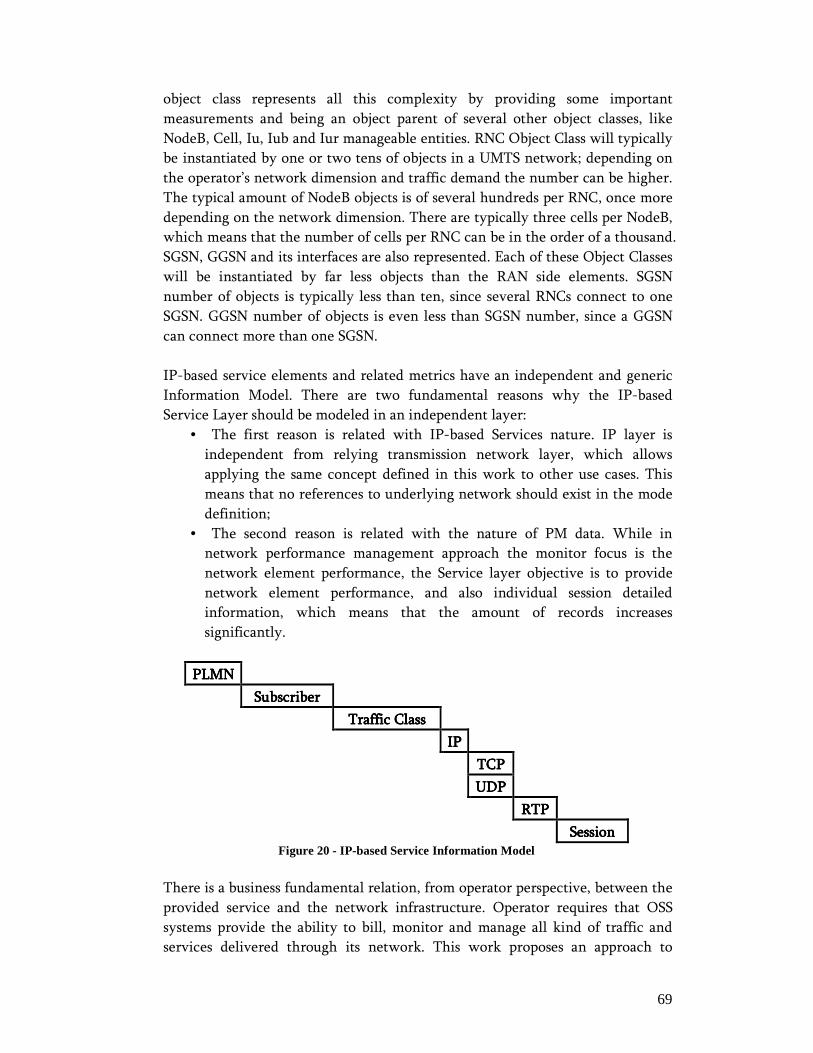
69
object class represents all this complexity by providing some important
measurements and being an object parent of several other object classes, like
NodeB, Cell, Iu, Iub and Iur manageable entities. RNC Object Class will typically
be instantiated by one or two tens of objects in a UMTS network; depending on
the operator’s network dimension and traffic demand the number can be higher.
The typical amount of NodeB objects is of several hundreds per RNC, once more
depending on the network dimension. There are typically three cells per NodeB,
which means that the number of cells per RNC can be in the order of a thousand.
SGSN, GGSN and its interfaces are also represented. Each of these Object Classes
will be instantiated by far less objects than the RAN side elements. SGSN
number of objects is typically less than ten, since several RNCs connect to one
SGSN. GGSN number of objects is even less than SGSN number, since a GGSN
can connect more than one SGSN.
IP-based service elements and related metrics have an independent and generic
Information Model. There are two fundamental reasons why the IP-based
Service Layer should be modeled in an independent layer:
• The first reason is related with IP-based Services nature. IP layer is
independent from relying transmission network layer, which allows
applying the same concept defined in this work to other use cases. This
means that no references to underlying network should exist in the mode
definition;
• The second reason is related with the nature of PM data. While in
network performance management approach the monitor focus is the
network element performance, the Service layer objective is to provide
network element performance, and also individual session detailed
information, which means that the amount of records increases
significantly.
PLMNPLMNPLMNPLMN
SubscriberSubscriberSubscriberSubscriber
Traffic ClassTraffic ClassTraffic ClassTraffic Class
IPIPIPIP
TCPTCPTCPTCP
UDPUDPUDPUDP
RTPRTPRTPRTP
SessionSessionSessionSession Figure 20 - IP-based Service Information Model
There is a business fundamental relation, from operator perspective, between the
provided service and the network infrastructure. Operator requires that OSS
systems provide the ability to bill, monitor and manage all kind of traffic and
services delivered through its network. This work proposes an approach to

70
enable such kind of feature, which is to relate the service specific information
with the PLMN specific information. So, in order to enable cross-layer IP-based
service monitoring capabilities, the corresponding service information model
must be related with the PLMN object class. This also enables the capacity to
report each element performance correlated with session performance specific
information taken from the same instant.
The Subscriber entity must be directly related with PLMN object class, since this
way it can be translated the business fundamental relation that exists between
operator infrastructure and service user. There is also a logical explanation for
this relation and has to due with the concept that all network activity
description is an abstraction of the overall subscriber activity, since the total
network activity is a sum of each subscriber activity, profile and behavior.
The remaining of the model describes the information hierarchy defined to
describe each individual session, i.e., each session is related with a UMTS traffic
class and related QoS parameters; in the other hand, for every single session
there are collected IP, TCP or UDP and RTP metrics.
71
3333....6666.... Key Performance IndicatorsKey Performance IndicatorsKey Performance IndicatorsKey Performance Indicators
Key performance indicators (KPIs) are a set of selected indicators used for
measuring the current network performance and trends. KPIs highlight the key
factors of network monitoring and warn in time of potential problems. KPIs are
also used for prioritizing the corrective actions.
A KPI can simply be equal to a Counter or to an arithmetic abstraction of
counters that can be applied to monitor a certain part of the network,
functionality or protocol.
ITU-T has defined in the standard E.800 some network monitoring KPI classes
that are applied in this work:
• Accessibility – can be defined as the probability that a service can be
obtained within specified tolerances and other given operating
conditions when requested by the user.
• Integrity – can be defined as the degree to which a service is provided
without excessive impairments, once obtained.
• Retainibility – can be defined as the probability that a service, once
obtained, will continue to be provided under given conditions for a
given time duration.
• Mobility – serves to monitor the performance mobility aspects (e.g.,
handover, location updates) and the degree of impact on network
overall behavior.
• Usage – serves to evaluate the network usage and capacity
performance (e.g., traffic volume, CPU usage, etc) and their impact on
overall network behavior.
All the KPIs explained in this chapter are based on the earlier described
measurements and counters. These KPIs were selected to provide all the
necessary information about end-to-end network performance and ability to
deliver IP-based services. All UTRAN related KPIs are a result of my daily work
and were defined and proposed by me. The Core Network KPIs selection results
from a research work on available defined KPIs. All the Service Layer KPIs were
defined for the purpose of this work.
UMTS Network functionalities can be split using several different approaches. In
this work the network analysis is done by dividing the network like in the
following:
• Radio Access Network and Core Network division: these are two very
distinct and independent parts of the network as already mentioned in
Chapter 2.2;

72
• Control Plane and User Plane: analyzing the network from an end-to-
end perspective, there is also the possibility to split into these two
functional parts. Network’s control plane is responsible for all the
signaling between elements and protocol procedures, and data plane is
responsible for the end-user data transmission;
• Cross-Layer Stack: this organization of network’s functionalities allows
abstract information about protocol layers, network elements and
procedures into logical layers. This approach provides the flexibility to
shape the performance information according to the analysis goal.
3333....6666....1111.... Network Session Network Session Network Session Network Session –––– Control Plane KPIs Control Plane KPIs Control Plane KPIs Control Plane KPIs
The Network session control plane part is split into independent phases:
Accessibility and Retainibility. The Accessibility part focuses on the ability to
access the network and establish a call. The Retainibility part is mainly
related with the network capacity to retain a call until it is normally released.
In this section it is presented a list of the most important network session
control plane KPIs. The way these are presented follows this logic:
o First step is to list the higher layer KPIs, i.e., those related with the
Packet Session layer;
o Follows the network service layer KPIs that are related with the
several signaling phases that compounds a packet session
procedure;
o The third step lists the network service KPIs detailed per failure
causes.
Packet Call Accessibility related KPIs:Packet Call Accessibility related KPIs:Packet Call Accessibility related KPIs:Packet Call Accessibility related KPIs:
Packet Call Setup Success Ratio – provides information about the probability
to establish successfully a connection with the network. This KPI combines
the probability to establish a RRC connection, followed by a Radio Access
Bearer, which means that both RAN and CN performance influence its result.
[ ][ ] %100*
][
][
allpeAttrabEstabTy
allpeSuccrabEstabTy
alltrrcEstabAt
allccrrcEstabSuPCSSR ∗=
Where all refers that all the PS connection types must be included in the
formula calculation. PS connection type refers to the traffic class associated
with the call establishment and can be one of the following:
• PS Interactive;
• PS Background;
• PS Streaming.

73
This KPI can be further detailed per traffic type, as follows:
( ) [ ][ ] %100*
],[
],[
,
,
jipeAttrabEstabTy
jipeSuccrabEstabTy
jitrrcEstabAt
jiccrrcEstabSuiNRTPCSSR ∗=∑
,
i refers to the traffic class.
i=0 -> instantiates the Interactive traffic class counter;
i=1 -> instantiates the Background traffic class counter.
( ) [ ][ ] %100*
][
][
kpeAttrabEstabTy
kpeSuccrabEstabTy
ktrrcEstabAt
kccrrcEstabSukRTPCSSR ∗=∑
k refers to the traffic class.
k=3 -> instantiates the Streaming traffic class counter;
Packet Session Setup Success Ratio – this KPI monitors the RAN ability to
establish a packet session. This KPI result is only influenced by RAN
performance as it provides information about the channel allocation
probability for PS traffic. The HS-DSCH, E-DCH and DCH successful
allocations are compared to all the allocation attempts. This KPI can also be
detailed per channel type, providing individually the HSDPA PSSR, HSUPA
PSSR and R99 PSSR, which is important to assess each channel contribution
for the overall result. Figure 21 shows a graphical representation of this KPI
results taken from a real live network.
[ ][ ] %100*
,,
allelAllocAtttransChann
jicelAllocSuctransChannjiPSSSR ∑=
i refers to the type of channel allocation and j to the traffic class.
For instance:
i=0, j=0 -> instantiates the HS-DSCH/E-DCH channel for
Interactive traffic class attempt counter;
i=1, j=1 -> instantiates the HS-DSCH/DCH channel for
Background traffic class attempt counter;
i=2, j=2 -> instantiates the DCH/DCH channel for Streaming
traffic class attempt counter;

74
Packet Session Success Ratio
91,00
92,00
93,00
94,00
95,00
96,00
97,00
08-07-2009
09-07-2009
10-07-2009
11-07-2009
12-07-2009
13-07-2009
14-07-2009
15-07-2009
16-07-2009
17-07-2009
18-07-2009
19-07-2009
20-07-2009
21-07-2009
22-07-2009
Day
Per
cent
(%
)
Figure 21 - Packet Session Setup Success Ratio daily evolution taken from a real live network
Packet Session Setup Failure Ratio detailed per Cause – this KPI group details
the probability of call rejection due to a specific reason. It is used to identify
the root cause of access problems. These KPIs can be influenced by causes
originated both in RAN and CN, which are:
• Admission Control rejections, which indicates degradation of radio
conditions mainly of DL codes, power and UL interference;
• Node B rejections mainly related with lack of hardware resources;
• DMCU rejections indicates the lack of RNC User Plane resources;
• Transport rejections mainly related with Iub congestion;
• Iu rejections are related with CN rejection;
• UE rejections related with user equipment problems;
• Other rejections reasons that are not contemplated in the earlier
counters.
Figure 22 shows a graphical representation of this KPI set, with results taken
from a real live network.
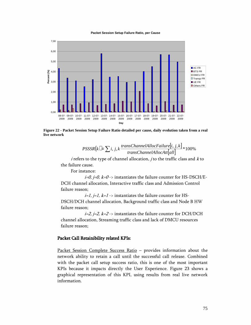
75
Packet Session Setup Failure Ratio, per Cause
0,00
1,00
2,00
3,00
4,00
5,00
6,00
7,00
08-07-2009
09-07-2009
10-07-2009
11-07-2009
12-07-2009
13-07-2009
14-07-2009
15-07-2009
16-07-2009
17-07-2009
18-07-2009
19-07-2009
20-07-2009
21-07-2009
22-07-2009
Day
Per
cent
(%
)
AC FRBTS FRDMCU FR
Transp FRUE FROthers FR
Figure 22 - Packet Session Setup Failure Ratio detailed per cause, daily evolution taken from a real live network
( ) [ ][ ] %100*
,,,,
allelAllocAtttransChann
kjilureelAllocFaitransChannkjikPSSSR ∑=
i refers to the type of channel allocation, j to the traffic class and k to
the failure cause.
For instance:
i=0, j=0, k=0 -> instantiates the failure counter for HS-DSCH/E-
DCH channel allocation, Interactive traffic class and Admission Control
failure reason;
i=1, j=1, k=1 -> instantiates the failure counter for HS-
DSCH/DCH channel allocation, Background traffic class and Node B HW
failure reason;
i=2, j=2, k=2 -> instantiates the failure counter for DCH/DCH
channel allocation, Streaming traffic class and lack of DMCU resources
failure reason;
Packet Call Retainibility related KPIs:Packet Call Retainibility related KPIs:Packet Call Retainibility related KPIs:Packet Call Retainibility related KPIs:
Packet Session Complete Success Ratio – provides information about the
network ability to retain a call until the successful call release. Combined
with the packet call setup success ratio, this is one of the most important
KPIs because it impacts directly the User Experience. Figure 23 shows a
graphical representation of this KPI, using results from real live network
information.
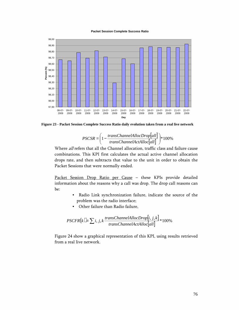
76
Packet Session Complete Success Ratio
97,90
98,00
98,10
98,20
98,30
98,40
98,50
98,60
98,70
98,80
98,90
99,00
08-07-2009
09-07-2009
10-07-2009
11-07-2009
12-07-2009
13-07-2009
14-07-2009
15-07-2009
16-07-2009
17-07-2009
18-07-2009
19-07-2009
20-07-2009
21-07-2009
22-07-2009
Day
Per
cent
(%
)
Figure 23 - Packet Session Complete Success Ratio daily evolution taken from a real live network
[ ][ ] %100*1
−=allelActAlloctransChann
allpelAllocDrotransChannPSCSR
Where all refers that all the Channel allocation, traffic class and failure cause
combinations. This KPI first calculates the actual active channel allocation
drops rate, and then subtracts that value to the unit in order to obtain the
Packet Sessions that were normally ended.
Packet Session Drop Ratio per Cause – these KPIs provide detailed
information about the reasons why a call was drop. The drop call reasons can
be:
• Radio Link synchronization failure, indicate the source of the
problem was the radio interface;
• Other failure than Radio failure,
( ) [ ][ ] %100*
,,,,
allelActAlloctransChann
kjipelAllocDrotransChannkjikPSCFR ∑=
Figure 24 show a graphical representation of this KPI, using results retrieved
from a real live network.

77
Packet Session Drop Ratio per Cause
0,00
0,50
1,00
1,50
2,00
2,50
08-07-
2009
09-07-
2009
10-07-
2009
11-07-
2009
12-07-
2009
13-07-
2009
14-07-
2009
15-07-
2009
16-07-
2009
17-07-
2009
18-07-
2009
19-07-
2009
20-07-
2009
21-07-
2009
22-07-
2009
Days
Per
cent
(%
)
HS-DSCH/E-DCH DR, RLHS-DSCH/DCH DR, RLDCH/DCH DR, RL
HS-DSCH/E-DCH DR, OtherHS-DSCH/DCH DR, OtherDCH/DCH DR, Other
Figure 24 - Packet Session Drop Ratio, detailed per affected channel and release cause, daily evolution taken from a real live network
Service AcService AcService AcService Accessibility related KPIs:cessibility related KPIs:cessibility related KPIs:cessibility related KPIs:
RRC Establishment Success Ratio – this KPI provides information about the
probability of RRC connection is established successfully. It is an important
KPI that is used to determine if RRC connection procedure is affecting
negatively the overall packet call setup process.
100%*t[all]rrcEstabAt
cc[all]rrcEstabSuRrcEstabSR=
Where all refers that all the PS connection types must be included in the
formula calculation. PS connection type refers to the traffic class associated
with the call establishment and can be one of the following:
• PS Interactive;
• PS Background;
• PS Streaming.
RRC Establishment Failure Ratio detailed per cause – this KPI group provides
information about the probability of RRC connection fails to establish
successfully due to all the possible failure reasons. It is important to analyze
this KPI group if the overall RRC connection establishment procedure is
affecting negatively the overall packet call setup process.
100%*t[all]rrcEstabAt
cc[i]rrcEstabSu(i)RrcEstabFR =
Where i refer to the individual failure cause, which can be the following:
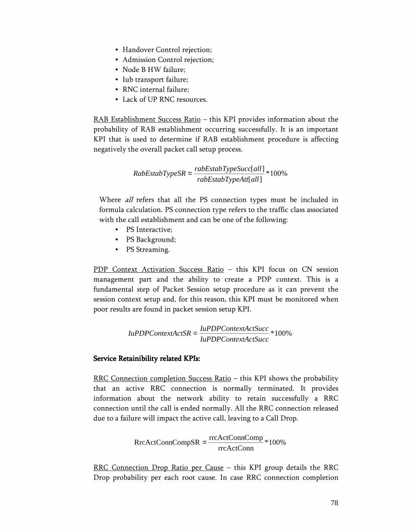
78
• Handover Control rejection;
• Admission Control rejection;
• Node B HW failure;
• Iub transport failure; • RNC internal failure; • Lack of UP RNC resources.
RAB Establishment Success Ratio – this KPI provides information about the
probability of RAB establishment occurring successfully. It is an important
KPI that is used to determine if RAB establishment procedure is affecting
negatively the overall packet call setup process.
%100*][
][
allpeAttrabEstabTy
allpeSuccrabEstabTypeSRRabEstabTy =
Where all refers that all the PS connection types must be included in
formula calculation. PS connection type refers to the traffic class associated
with the call establishment and can be one of the following:
• PS Interactive;
• PS Background;
• PS Streaming.
PDP Context Activation Success Ratio – this KPI focus on CN session
management part and the ability to create a PDP context. This is a
fundamental step of Packet Session setup procedure as it can prevent the
session context setup and, for this reason, this KPI must be monitored when
poor results are found in packet session setup KPI.
%100*xtActSuccIuPDPConte
xtActSuccIuPDPContextActSRIuPDPConte =
Service Retainibility related KPIs:Service Retainibility related KPIs:Service Retainibility related KPIs:Service Retainibility related KPIs:
RRC Connection completion Success Ratio – this KPI shows the probability
that an active RRC connection is normally terminated. It provides
information about the network ability to retain successfully a RRC
connection until the call is ended normally. All the RRC connection released
due to a failure will impact the active call, leaving to a Call Drop.
100%*rrcActConn
ComprrcActConnCompSRRrcActConn =
RRC Connection Drop Ratio per Cause – this KPI group details the RRC
Drop probability per each root cause. In case RRC connection completion

79
ratio presents a low value, these KPIs must be monitored to assess what is the
reason of such problem.
100%*rrcActConn
Drop[i]rrcActConni)DropRatio(RrcActConn =
Where i refers to the individual failure cause, which can be the following:
• Radio interface failure; • Node B HW failure;
• User Equipment failure;
• Iu interface failure; • Iur interface failure; • RNC internal failure; • Security Mode Control rejections.
RAB Complete Success Ratio – this KPI focus on the RAB Active phase of a
call and provides information about the probability of an Active RAB be
released normally. Figure 25 shows a graphical representation using real live
network data.
100%*rabActConn
ComprabActConnCompSRRabActConn =
RAB Complete Success Ratio
97,60
97,80
98,00
98,20
98,40
98,60
98,80
99,00
08-07-2009
09-07-2009
10-07-2009
11-07-2009
12-07-2009
13-07-2009
14-07-2009
15-07-2009
16-07-2009
17-07-2009
18-07-2009
19-07-2009
20-07-2009
21-07-2009
22-07-2009
Day
Per
cent
(%
)
Figure 25 - RAB Complete SR, daily evolution taken from a real live network
RAB Drop Ratio per Cause – this KPI group shows the RAB Drop probability
detailed per failure cause. In case RAB Complete SR presents a low value,
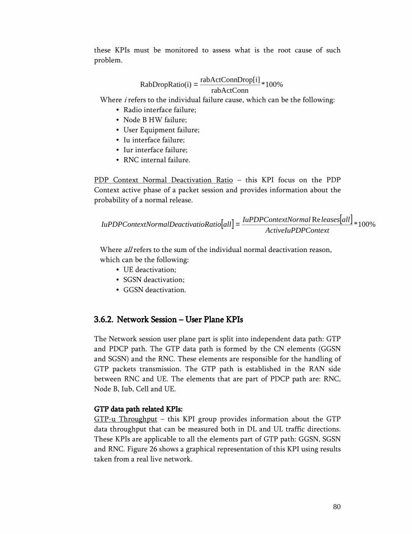
80
these KPIs must be monitored to assess what is the root cause of such
problem.
100%*rabActConn
Drop[i]rabActConnio(i)RabDropRat =
Where i refers to the individual failure cause, which can be the following:
• Radio interface failure; • Node B HW failure;
• User Equipment failure;
• Iu interface failure; • Iur interface failure; • RNC internal failure.
PDP Context Normal Deactivation Ratio – this KPI focus on the PDP
Context active phase of a packet session and provides information about the
probability of a normal release.
[ ] [ ]%100*
Re
PContextActiveIuPD
allleasesxtNormalIuPDPConteallatioactivatioRxtNormalDeIuPDPConte =
Where all refers to the sum of the individual normal deactivation reason,
which can be the following:
• UE deactivation; • SGSN deactivation; • GGSN deactivation.
3333....6666....2222.... Network Session Network Session Network Session Network Session –––– User Plane KPIs User Plane KPIs User Plane KPIs User Plane KPIs
The Network session user plane part is split into independent data path: GTP
and PDCP path. The GTP data path is formed by the CN elements (GGSN
and SGSN) and the RNC. These elements are responsible for the handling of
GTP packets transmission. The GTP path is established in the RAN side
between RNC and UE. The elements that are part of PDCP path are: RNC,
Node B, Iub, Cell and UE.
GTP data path related KPIs:GTP data path related KPIs:GTP data path related KPIs:GTP data path related KPIs:
GTP-u Throughput – this KPI group provides information about the GTP
data throughput that can be measured both in DL and UL traffic directions.
These KPIs are applicable to all the elements part of GTP path: GGSN, SGSN
and RNC. Figure 26 shows a graphical representation of this KPI using results
taken from a real live network.
81
(Mbps) 1000000*60 * yPeriodGranularit
Volume[i]GTPu_Data_ * 8Thp(i)IuPS_GTPu_ =
Where i refers to traffic direction:
i=0 -> instantiates the DL traffic direction counter;
i=1 -> instantiates the UL traffic direction counter.
GranularityPeriod provides the measurement period in minutes, and
therefore there is the need to convert its value to seconds by multiplying by a
factor of 60 seconds.
GTPu_Data_Volume[i] provides the amount of Bytes transmitted over the Iu
interface between RNC, SGSN, and therefore, it must be multiplied by a
factor of 8 to convert its value for bits.
Iu-PS GTP-u Throughput
0,00
10,00
20,00
30,00
40,00
50,00
60,00
70,00
80,00
17-07-2009 18-07-2009 19-07-2009 20-07-2009 21-07-2009 22-07-2009 23-07-2009
Day
Thr
ough
put (
Mbi
t/s)
Iu-PS GTP-U DL
Iu-PS GTP-U UL
Figure 26 - RNC Iu-PS GTP-u Throughput, daily evolution from a real live network
GTP-u Traffic Volume – this KPI group provides information about the GTP
data volume that can be measured both in DL and UL traffic directions.
These KPIs are applicable to all the elements part of GTP path: GGSN, SGSN
and RNC.
(MB) 1000000
Volume[i]GTPu_Data_DataVol(i)IuPS_GTPu_ =
Where i refers to traffic direction:
i=0 -> instantiates the DL traffic direction counter;
i=1 -> instantiates the UL traffic direction counter.
82
GTPu_Data_Volume[i] provides the amount of Bytes transmitted over the Iu
interface between RNC and SGSN.
GTP-u Throughput detailed per traffic/bearer class – this KPI group provides
information about the GTP throughput that can be measured both in DL and
UL traffic directions, adding additional detail about the corresponding traffic
and bearer priority class. These KPIs are applicable to SGSN element in GTP
data path.
(Mbps) 1000000*60 * yPeriodGranularit
k]j,Volume[i,GTPu_Data_ * 8k)j,Thp(i,IuPS_GTPu_ =
Where i refers to the traffic class, j refers to the bearer type and k to the
traffic direction (DL or UL).
GTP-u Data Volume detailed per traffic/bearer class – this KPI group
provides detailed information about the GTP-u traffic volume transmitted for
each traffic class, bearer type association both in DL and UL directions. These
KPIs are applicable to SGSN element in GTP data path. Figure 27 shows a
graphical representation of this KPI set using results retrieved from a real live
network.
(MB) 1000000
k]j,Volume[i,GTPu_Data_k)j,DataVol(i,IuPS_GTPu_ =
Where i refers to the traffic class, j refers to the bearer type and k to the
traffic direction (DL or UL).
Iu Traffic Volume - Interactive THP2, 2Mbps
0,00
5.000,00
10.000,00
15.000,00
20.000,00
25.000,00
30.000,00
26-10-2009
27-10-2009
28-10-2009
29-10-2009
30-10-2009
31-10-2009
01-11-2009
02-11-2009
03-11-2009
04-11-2009
Day
Dat
a V
olum
e (M
B)
UL
DL
Figure 27 - SGSN Iu-PS GTP-u Data Volume detailed per traffic/bearer class, daily evolution from a real live network
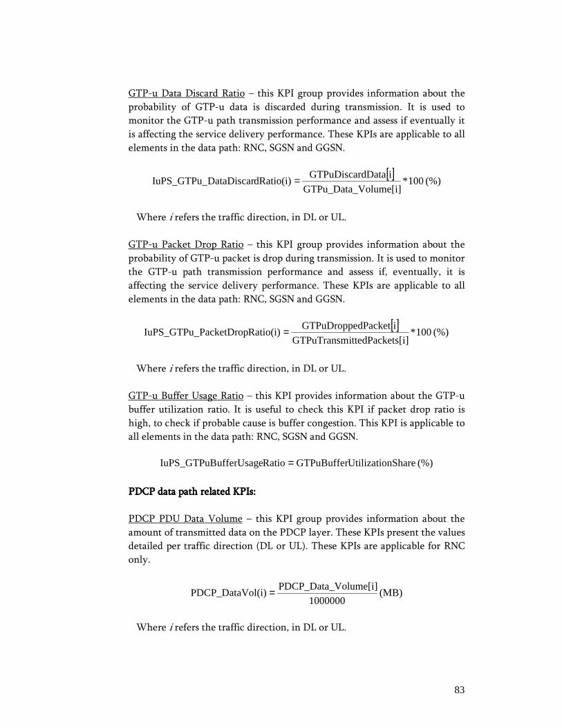
83
GTP-u Data Discard Ratio – this KPI group provides information about the
probability of GTP-u data is discarded during transmission. It is used to
monitor the GTP-u path transmission performance and assess if eventually it
is affecting the service delivery performance. These KPIs are applicable to all
elements in the data path: RNC, SGSN and GGSN.
[ ](%) 100 *
Volume[i]GTPu_Data_
idDataGTPuDiscardRatio(i)DataDiscarIuPS_GTPu_ =
Where i refers the traffic direction, in DL or UL.
GTP-u Packet Drop Ratio – this KPI group provides information about the
probability of GTP-u packet is drop during transmission. It is used to monitor
the GTP-u path transmission performance and assess if, eventually, it is
affecting the service delivery performance. These KPIs are applicable to all
elements in the data path: RNC, SGSN and GGSN.
[ ](%) 100 *
ts[i]ittedPackeGTPuTransm
idPacketGTPuDroppeRatio(i)PacketDropIuPS_GTPu_ =
Where i refers the traffic direction, in DL or UL.
GTP-u Buffer Usage Ratio – this KPI provides information about the GTP-u
buffer utilization ratio. It is useful to check this KPI if packet drop ratio is
high, to check if probable cause is buffer congestion. This KPI is applicable to
all elements in the data path: RNC, SGSN and GGSN.
(%) nShareUtilizatioGTPuBufferRatioufferUsageIuPS_GTPuB =
PDCP data path related KPIs:PDCP data path related KPIs:PDCP data path related KPIs:PDCP data path related KPIs:
PDCP PDU Data Volume – this KPI group provides information about the
amount of transmitted data on the PDCP layer. These KPIs present the values
detailed per traffic direction (DL or UL). These KPIs are applicable for RNC
only.
(MB) 1000000
Volume[i]PDCP_Data_ol(i)PDCP_DataV =
Where i refers the traffic direction, in DL or UL.
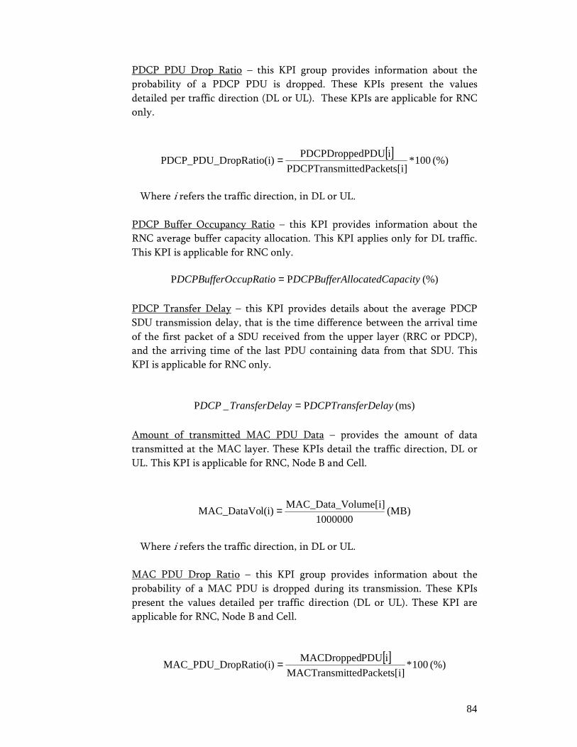
84
PDCP PDU Drop Ratio – this KPI group provides information about the
probability of a PDCP PDU is dropped. These KPIs present the values
detailed per traffic direction (DL or UL). These KPIs are applicable for RNC
only.
[ ](%) 100 *
ts[i]ittedPackePDCPTransm
idPDUPDCPDroppe)ropRatio(iPDCP_PDU_D =
Where i refers the traffic direction, in DL or UL.
PDCP Buffer Occupancy Ratio – this KPI provides information about the
RNC average buffer capacity allocation. This KPI applies only for DL traffic.
This KPI is applicable for RNC only.
(%) PP pacityllocatedCaDCPBufferAccupRatioDCPBufferO =
PDCP Transfer Delay – this KPI provides details about the average PDCP
SDU transmission delay, that is the time difference between the arrival time
of the first packet of a SDU received from the upper layer (RRC or PDCP),
and the arriving time of the last PDU containing data from that SDU. This
KPI is applicable for RNC only.
(ms) P_P rDelayDCPTransfelayTransferDeDCP =
Amount of transmitted MAC PDU Data – provides the amount of data
transmitted at the MAC layer. These KPIs detail the traffic direction, DL or
UL. This KPI is applicable for RNC, Node B and Cell.
(MB) 1000000
olume[i]MAC_Data_Vl(i)MAC_DataVo =
Where i refers the traffic direction, in DL or UL.
MAC PDU Drop Ratio – this KPI group provides information about the
probability of a MAC PDU is dropped during its transmission. These KPIs
present the values detailed per traffic direction (DL or UL). These KPI are
applicable for RNC, Node B and Cell.
[ ](%) 100 *
s[i]ttedPacketMACTransmi
iPDUMACDroppedopRatio(i)MAC_PDU_Dr =

85
Where i refers the traffic direction, in DL or UL.
Amount of transmitted FP frames – provides the amount of Frame Protocol
frames transmitted over Iub. These KPIs detail the traffic direction, DL or UL.
These KPIs are applicable for RNC and Node B.
(Nr) FP_PDUs[i]i)sFPframes(AmountTran Amount=
Where i refers the traffic direction, in DL or UL.
FP Drop Frames detail per channel – this KPI group provides information
about the probability of a FP frame is dropped during its transmission. These
KPIs present the values detailed per related transport channel, HS-DSCH, E-
DCH or DCH (in the case of being the HS-DSCH return channel). These KPIs
are applicable for RNC and Node B.
[ ](%) 100 *
i]tedFrames[FPTransmit
irameFPDroppedF)ropRatio(iFP_FRame_D =
Where i refers to the radio transport channels associated with the
transmitted FP frames.
i=0 -> instantiates the HS-DSCH transport channel counters;
i=1 -> instantiates the E-DCH transport channel counters;
i=2 -> instantiates the DCH transport channel counters;
MAC-hs Data Volume – provides the amount of correctly received MAC-hs
data volume at the Node B. This KPI is applicable for Node only.
( )(MB)
1000000 * 8
itsDiscMAChsB-tsRecMAChsBiolDSCH_DataV-HS =
HSDPA active Cell throughput – provides the average active HS-DSCH
MAC-d throughput, calculated as the HSDPA MAC-d throughput at BTS
divided by the active HS-DSCH transmission time. The active time refers to
the scheduled TTIs, i.e. when sending data. This KPI is applicable Cell only.
Figure 28 shows a graphical representation of this KPI using results from a
real live network.
( )(Mbps)
1000000 * IsmissionTTActiveTran
500*itsDiscMAChsB-tsRecMAChsBill_ThpDSCH_ActCe-HS =
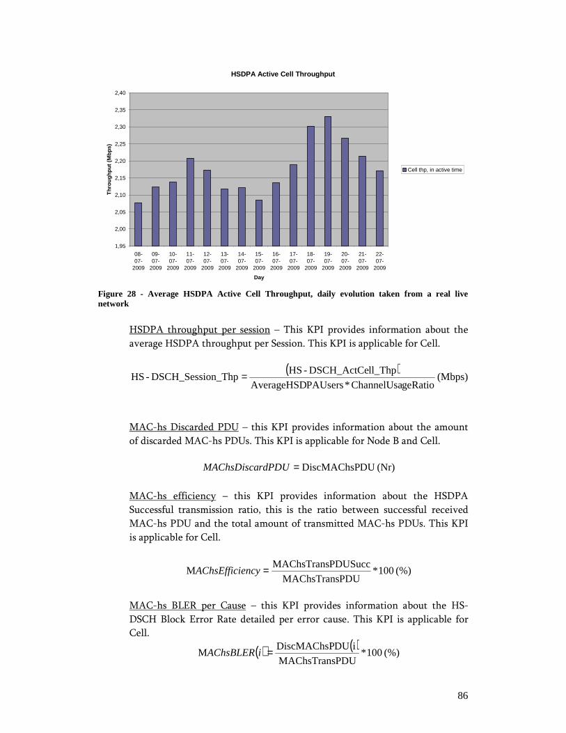
86
HSDPA Active Cell Throughput
1,95
2,00
2,05
2,10
2,15
2,20
2,25
2,30
2,35
2,40
08-07-
2009
09-07-
2009
10-07-
2009
11-07-
2009
12-07-
2009
13-07-
2009
14-07-
2009
15-07-
2009
16-07-
2009
17-07-
2009
18-07-
2009
19-07-
2009
20-07-
2009
21-07-
2009
22-07-
2009
Day
Thr
ough
put (
Mbp
s)
Cell thp, in active time
Figure 28 - Average HSDPA Active Cell Throughput, daily evolution taken from a real live network
HSDPA throughput per session – This KPI provides information about the
average HSDPA throughput per Session. This KPI is applicable for Cell.
( )(Mbps)
geRatioChannelUsa * PAUsersAverageHSD
ll_ThpDSCH_ActCe-HSon_ThpDSCH_Sessi-HS =
MAC-hs Discarded PDU – this KPI provides information about the amount
of discarded MAC-hs PDUs. This KPI is applicable for Node B and Cell.
(Nr) DUDiscMAChsP=rdPDUMAChsDisca
MAC-hs efficiency – this KPI provides information about the HSDPA
Successful transmission ratio, this is the ratio between successful received
MAC-hs PDU and the total amount of transmitted MAC-hs PDUs. This KPI
is applicable for Cell.
(%) 100 * PDUMAChsTrans
PDUSuccMAChsTransM =encyAChsEffici
MAC-hs BLER per Cause – this KPI provides information about the HS-
DSCH Block Error Rate detailed per error cause. This KPI is applicable for
Cell.
( ) ( )(%) 100 *
PDUMAChsTrans
iDUDiscMAChsPM =iAChsBLER

87
Where i refers to the error cause:
i=0 -> instantiates the Maximum Number of Retransmissions
counter;
i=1 -> instantiates the T1 Timer counter;
i=2 -> instantiates the Other Reason counter.
MAC-es Data Volume – provides the amount of transmitted MAC-es data
volume over the Cell. This KPI is applicable for Node B and Cell.
( )(MB)
1000000
olEDCH_DataVlDCH_DataVo-E =
HSUPA active Cell throughput – provides the average active E-DCH MAC-es
throughput, calculated as the total amount of MAC-es transmitted data at
Cell level divided by the active E-DCH transmission time. The active time
refers to the scheduled TTIs, i.e. when sending data. This KPI is applicable
for Cell.
(Mbps) 1000 * IsmissionTTActiveTran
8*DataEDCHtransmll_ThpEDCH_ActCe =
HSUPA throughput per session – This KPI provides information about the
average HSUPA throughput per Session. This KPI includes retransmitted data.
This KPI is applicable for Cell.
(Mbps) TimeEDCHTransm
8 * DataEDCHtransmon_ThpEDCH_Sessi =
MAC-es Discarded Frames – this KPI provides information about the amount
of discarded MAC-es frames. This KPI is applicable for RNC and Cell.
(Nr) ramesDiscMACesF=rdFramesMACesDisca
MAC-es efficiency – this KPI provides information about the HSUPA
Successful transmission ratio, this is the ratio between successful transmitted
MAC-es frames and the total amount of transmitted MAC-es frames. This
KPI value decreases with the need to increase the number of retransmission,
for instance due to radio conditions degradation. This KPI is applicable for
RNC and Cell.
(%) 100 * FramesMACesTrans
FramesSuccMACesTransM =encyACesEffici
88
MAC-es BLER per Cause – this KPI provides information about the E-DCH
Block Error Rate detailed per error cause. This KPI is applicable for Cell.
( ) ( )(%) 100 *
PDUMACesTrans
iDUDiscMACesPM =iACesBLER
Where i refers to the error cause:
i=0 -> instantiates the HARQ failure counter;
i=1 -> instantiates the Buffer Overflow;
i=2 -> instantiates the Other Reason counter.
3333....6666....3333.... Service Session Service Session Service Session Service Session –––– Service Performance Indicators Service Performance Indicators Service Performance Indicators Service Performance Indicators
The KPIs described in this session can also be found in [23]....
The Service Performance Indicator (SPI) is mainly affected by the on-path
links, nodes performance and the End-to-End conditions. It shows the
overall performance of a network according to the quality of the contained
service delivery.
The Revenue Factor (RF) has a direct implication on the evaluation of the
network adequacy to the services being provided. The under-performance of
voice should reflect a larger impact on the Network Adequacy Indicator (NAI)
to the services being delivered since it is a very profitable service.
Network Adequacy Indicator – this KPI provides information about the
ability of a specific network to support the delivery of a given service. This
formula can be applied for any network and service combination.
It is composed by a Revenue Factor (RF) that is an operator configurable
factor that translates the revenue importance of a specific service in the
overall operator business.
( )( ) ( )( ) iRF
*iRF∑=
cesTotalServi
i
iSPIiNAI
Where i refers to the type of service instance, for instance:
• VoIP;
• Video;
• Gaming;
• IPTV;
• Browsing;
• etc.
Service Performance Indicator – this KPI provides a weighted average
between, the importance of a given KPI to a certain service, and the rating
that the same KPI achieves. The SPI depends on the type of service, for
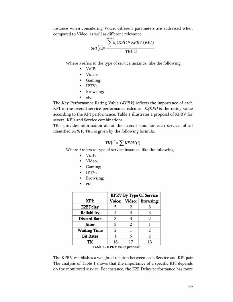
89
instance when considering Voice, different parameters are addressed when
compared to Video, as well as different relevance.
( ) ( ) iTK
)()(∑ ×=
AllKPIs
iii KPIKPRVKPIk
iSPI
Where i refers to the type of service instance, like the following:
• VoIP;
• Video;
• Gaming;
• IPTV;
• Browsing;
• etc.
The Key Performance Rating Value (KPRV) reflects the importance of each
KPI to the overall service performance calculus. Ki(KPI) is the rating value
according to the KPI performance. Table 1 illustrates a proposal of KPRV for
several KPIs and Service combinations.
TK(i) provides information about the overall sum, for each service, of all
identified KPRV. TK(i) is given by the following formula:
( ) ∑= )(iKPRViTK
Where i refers to type of service instance, like the following:
• VoIP;
• Video;
• Gaming;
• IPTV;
• Browsing;
• etc.
KPRV By Type Of ServiKPRV By Type Of ServiKPRV By Type Of ServiKPRV By Type Of Servicececece
KPI:KPI:KPI:KPI: Voice:Voice:Voice:Voice: Video:Video:Video:Video: Browsing:Browsing:Browsing:Browsing:
E2EDelayE2EDelayE2EDelayE2EDelay 5 2 3
ReliabilityReliabilityReliabilityReliability 4 4 3
Discard RateDiscard RateDiscard RateDiscard Rate 3 3 2
JitterJitterJitterJitter 3 2 1
Waiting TimeWaiting TimeWaiting TimeWaiting Time 2 1 2
Bit RatesBit RatesBit RatesBit Rates 1 5 2
TKTKTKTK 18 17 13 Table 1 - KPRV value proposal
The KPRV establishes a weighted relation between each Service and KPI pair.
The analysis of Table 1 shows that the importance of a specific KPI depends
on the monitored service. For instance, the E2E Delay performance has more

90
impact on Voice services then for Video and this fact is reflected in the KPI
classified weight that is higher for Voice than for Video, and also is the KPI
with higher weighted value within Voice classification. In the other hand,
the most important factor impacting Video performance is the network
capability to provide the required Bit Rate; this is reflected in the highest
weighted value for Video classification. In the case of available Bit Rate KPI,
for Voice service, it is the least important factor to be considered in overall
performance evaluation.
Table 2 defines the service rating value (R Value) according to defined
threshold for each KPI.
RRRR DelayDelayDelayDelay
(ms)(ms)(ms)(ms)
Jitter (ms)Jitter (ms)Jitter (ms)Jitter (ms) Discard Discard Discard Discard
Rate (%)Rate (%)Rate (%)Rate (%)
Reliability (%)Reliability (%)Reliability (%)Reliability (%) WT (s)WT (s)WT (s)WT (s)
5555 <50 <0.1xDelay <0.001 >99.999 <0.01
4444 [50;100] [0.1D;0.5D] [0.001;0.0
1]
[99.99;99.998] [0.001;0.1]
3333 [100;150] [0.5D;0.8D] [0.01;0.1] [99.9;99.999] [0.1;1]
2222 [150;300] [0.8D;D] [0.1;1] [99.9;99] [1;10]
1111 [300;600] [D;2D] [1;10] [90;99] [10;100]
0000 > 600 >2D >10 <90 >100 Table 2 – Rating Value according to service behavior defined thresholds
Table 2 establishes, for each Service KPI, a rating value R according to the
threshold rank defined to classify the network measured performance. For
instance, in the case the network measured Delay is lower than 50 (ms), the
rating value is equal to 5 and 0 if the measured result is higher than 600 (ms).
In the other hand, a network Reliability performance value higher than
99.999 (%) corresponds to a rating value R equal to 5, in turn a measured
result lower than 90 (%) corresponds to a R value equal to 0.
Applying to the defined SPI formula, the values defined in table 1 for KPRV
and in table 2 for R value, it results in a final formula of the following form:
( ) ( )
××=
voice
voice
mvoice
TK
TK
RBRKPRVREDKPRVESPI ML /2 111
In Section 3.7 the Service Performance Indicator Analysis reporting use case
provides an example of this KPI classification usage.

91
3333....7777.... ReportsReportsReportsReports
A report is a logical association of KPIs and PIs that aim to provide means to take
conclusions in the end of the analysis. The reports proposed in this work extend
the current available reports, by combining data that not only describes the end-
to-end network behavior, but also relates the network layer statistics with the
IP-based Service layer statistics.
IPIPIPIP----based Service Report Use Casesbased Service Report Use Casesbased Service Report Use Casesbased Service Report Use Cases
Packet Loss AnalysisPacket Loss AnalysisPacket Loss AnalysisPacket Loss Analysis
The first reporting use case is designed to provide an analysis flow for IP-based
Service Monitoring and detect problems related with service layer only, i.e.,
problems that are not originated by network performance degradation. This
report group is called “Service Awareness”.
Please note that the data shown in the following reports is not real and was
produced for this Use Case demonstration.
The first report begins to detail the session context in a dashboard fashion. The
following figure shows how the initial dashboard of “Session Description Report”
is organized.
© Nokia Siemens Networks
SIP Session details
RTCP details
IP details
GTP details
PDCP details
Service AwarenessSession Description Report
IMSI: 310150122534141
Session ID: 543367GGSN Address: ISN-BH APN Name: www.skype.com
Creation Time: 23-07-2009 16:23:34
Closed Time: 23-07-2009 16:28:56
PDP Address: 10.49.48.124 SIP Session ID: 2890844527
Figure 29 - Service Awareness – Session Description Report, Initial Dashboard
User can click on one of the following buttons, and browse for more details:
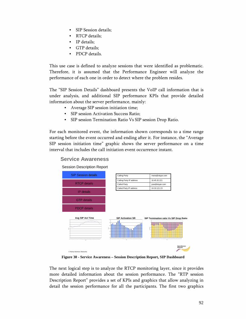
92
• SIP Session details;
• RTCP details;
• IP details;
• GTP details;
• PDCP details.
This use case is defined to analyze sessions that were identified as problematic.
Therefore, it is assumed that the Performance Engineer will analyze the
performance of each one in order to detect where the problem resides.
The “SIP Session Details” dashboard presents the VoIP call information that is
under analysis, and additional SIP performance KPIs that provide detailed
information about the server performance, mainly:
• Average SIP session initiation time;
• SIP session Activation Success Ratio;
• SIP session Termination Ratio Vs SIP session Drop Ratio.
For each monitored event, the information shown corresponds to a time range
starting before the event occurred and ending after it. For instance, the “Average
SIP session initiation time” graphic shows the server performance on a time
interval that includes the call initiation event occurrence instant.
© Nokia Siemens Networks
SIP Session details
24.33.121.23Called Party IP address
[email protected] Party
10.45.32.221Calling Party IP address
[email protected] Party
RTCP details
IP details
GTP details
PDCP details
Service AwarenessSession Description Report
0
1
2
3
4
5
6
7
8
0:00:00
1:00:00
2:00:00
3:00:00
4:00:00
5:00:00
6:00:00
7:00:00
8:00:00
9:00:00
10:00:00
11:00:
00
12:00:00
13:00:00
14:00:00
15:00
:00
16:00:00
17:00:00
18:00:
00
19:00
:00
20:00
:00
21:00:
00
22:00:
00
23:00
:00
Hour
Tim
e (S
)
Avg SIP Act Time
97,00
97,50
98,00
98,50
99,00
99,50
100,00
0:00:0
0
1:00:0
0
2:00:0
0
3:00:0
0
4:00:0
0
5:00:0
0
6:00:0
0
7:00:0
0
8:00:0
0
9:00:0
0
10:00:00
11:00
:00
12:00
:00
13:00:0
0
14:00:0
0
15:00
:00
16:00:0
0
17:00:0
0
18:00:00
19:00:00
20:00
:00
21:00:00
22:00:00
23:00
:00
Hour
Tim
e (S
)
SIP Activation SR
88
90
92
94
96
98
100
102
0:00:00
1:00:00
2:00:00
3:00:00
4:00:00
5:00:00
6:00:00
7:00:00
8:00:00
9:00:00
10:00:00
11:00:00
12:00
:00
13:00
:00
14:00
:00
15:00
:00
16:00
:00
17:00
:00
18:00
:00
19:00
:00
20:00:00
21:00:00
22:00:00
23:00:00
Hour
Per
cen
tag
e (%
)
SIP Termination ratio Vs SIP Drop Ratio
Figure 30 - Service Awareness – Session Description Report, SIP Dashboard
The next logical step is to analyze the RTCP monitoring layer, since it provides
more detailed information about the session performance. The “RTP session
Description Report” provides a set of KPIs and graphics that allow analyzing in
detail the session performance for all the participants. The first two graphics

93
show the relation between the amount of lost packets when compared with the
amount of sent packets. The first graph details the absolute values of sent and
lost packets, and the second one details the actual relative “Packet Drop Ratio”
value. The third graphic provides information about the average session End-to-
End Delay and average Jitter. In the other hand, the fourth and fifth graphics
provide information related with the user experienced sound quality detailed by
the “Voice Signal Power”, “Noise Level” and “Distortion Level”.
The detailed analysis of this dashboard would indicate that the session was
affected by the “Packet Loss Ratio” effect that, for one of the participants, is
frequently above 2% along the session duration, which affects significantly the
MOS calculated for this session, which also can be seen in the RTCP dashboard.
So, this would imply to analyze the next lower layer (IP layer) performance in
order to assess where the problem source is.
© Nokia Siemens Networks
Service AwarenessRTP Session Description Report
13MoS
[email protected]@skype.com
60 20R-Value
SIP Session details
RTCP details
IP details
GTP details
PDCP details
0
1000
2000
3000
4000
5000
6000
7000
16:24:00 16:24:30 16:25:00 16:25:30 16:26:00 16:26:30 16:27:00 16:27:30 16:28:00 16:28:30 16:28:56
Time
Pac
ket S
ent (
#)
Packets : Sent Vs Drop
0
1
2
3
4
5
6
16:24:00 16:24:30 16:25:00 16:25:30 16:26:00 16:26:30 16:27:00 16:27:30 16:28:00 16:28:30 16:28:56
Time
Dro
p R
atio
(%)
Packet Drop Ratio
0
50
100
150
200
250
300
16:24:00 16:24:30 16:25:00 16:25:30 16:26:00 16:26:30 16:27:00 16:27:30 16:28:00 16:28:30 16:28:56
Time
E2E
Del
ay (m
s)
Delay /Jitter
0
5
10
15
20
25
30
35
40
45
16:24:00 16:24:30 16:25:00 16:25:30 16:26:00 16:26:30 16:27:00 16:27:30 16:28:00 16:28:30 16:28:56
Time
No
ise
Leve
l (d
B)
Voice SigPower Vs Noise Level
0
10
20
30
40
50
60
16:24:00 16:24:30 16:25:00 16:25:30 16:26:00 16:26:30 16:27:00 16:27:30 16:28:00 16:28:30 16:28:56
Time
Dis
torti
on
Leve
l (%
)
Distortion Level
Figure 31 - Service Awareness– Session Description Report, RTP Dashboard
The analysis of the “IP session Description Report” dashboard enables to
conclude that the IP layer shows the same pattern behavior as shown at the RTP
layer. This allows concluding that the problem source is due to any specific RTP
layer factor.
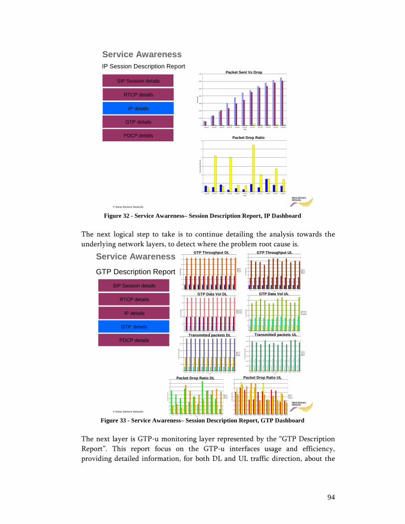
94
© Nokia Siemens Networks
Service AwarenessIP Session Description Report
SIP Session details
RTCP details
IP details
GTP details
PDCP details
0
1000
2000
3000
4000
5000
6000
7000
16:24:00 16:24:30 16:25:00 16:25:30 16:26:00 16:26:30 16:27:00 16:27:30 16:28:00 16:28:30 16:28:56
Time
Pa
cket
s (#
)
Packet Sent Vs Drop
0
1
2
3
4
5
6
16:24:00 16:24:30 16:25:00 16:25:30 16:26:00 16:26:30 16:27:00 16:27:30 16:28:00 16:28:30 16:28:56
Time
Pac
kets
Dro
p R
atio
(%)
Packet Drop Ratio
Figure 32 - Service Awareness– Session Description Report, IP Dashboard
The next logical step to take is to continue detailing the analysis towards the
underlying network layers, to detect where the problem root cause is.
© Nokia Siemens Networks
Service Awareness
GTP Description Report
SIP Session details
RTCP details
IP details
GTP details
PDCP details
0,00
10,00
20,00
30,00
40,00
50,00
60,00
70,00
Time 16:00:00 16:05:00 16:10:00 16:15:00 16:20:00 16:25:00 16:30:00 16:35:00 16:40:00 16:45:00 16:50:00
Time
Thr
ough
put (
Mbp
s) RNC
SGSN
GGSN
GTP Throughput DL
0
500
1000
1500
2000
2500
16:00:00 16:05:00 16:10:00 16:15:00 16:20:00 16:25:00 16:30:00 16:35:00 16:40:00 16:45:00 16:50:00 16:55:00
Time
Dat
a V
olu
me
(Mbp
s) RNC (MB)
SGSN (MB)
GGSN (MB)
GTP Data Vol DL
0
500000
1000000
1500000
2000000
2500000
16:00:00 16:05:00 16:10:00 16:15:00 16:20:00 16:25:00 16:30:00 16:35:00 16:40:00 16:45:00 16:50:00 16:55:00
Time
Tran
smitt
ed
Pa
cke
ts (M
bps)
RNC
SGSN
GGSN
Transmitted packets DL
0
0,2
0,4
0,6
0,8
1
1,2
1,4
1,6
1,8
16:00:00 16:05:00 16:10:00 16:15:00 16:20:00 16:25:00 16:30:00 16:35:00 16:40:00 16:45:00 16:50:00 16:55:00
Time
Pac
kets
Dro
p R
atio
(%)
RNC
SGSN
GGSN
Packet Drop Ratio DL
0
2
4
6
8
10
12
14
16
18
20
16:00:00 16:05:00 16:10:00 16:15:00 16:20:00 16:25:00 16:30:00 16:35:00 16:40:00 16:45:00 16:50:00 16:55:00
Time
Thro
ughp
ut (M
bps
)
RNC
SGSN
GGSN
GTP Throughput UL
0
100
200
300
400
500
600
700
16:00:00 16:05:00 16:10:00 16:15:00 16:20:00 16:25:00 16:30:00 16:35:00 16:40:00 16:45:00 16:50:00 16:55:00
Time
Dat
a V
olum
e (M
bps
)
RNC (MB)
SGSN (MB)
GGSN (MB)
GTP Data Vol UL
0
100000
200000
300000
400000
500000
600000
700000
16:00:00 16:05:00 16:10:00 16:15:00 16:20:00 16:25:00 16:30:00 16:35:00 16:40:00 16:45:00 16:50:00 16:55:00
Time
Tra
nsm
itted
Pac
kets
(Mbp
s)
RNC
SGSN
GGSN
Transmitted packets UL
0
0,2
0,4
0,6
0,8
1
1,2
1,4
1,6
16:00:00 16:05:00 16:10:00 16:15:00 16:20:00 16:25:00 16:30:00 16:35:00 16:40:00 16:45:00 16:50:00 16:55:00
Time
Pac
kets
Dro
p R
atio
(%)
RNC
SGSN
GGSN
Packet Drop Ratio UL
Figure 33 - Service Awareness– Session Description Report, GTP Dashboard
The next layer is GTP-u monitoring layer represented by the “GTP Description
Report”. This report focus on the GTP-u interfaces usage and efficiency,
providing detailed information, for both DL and UL traffic direction, about the
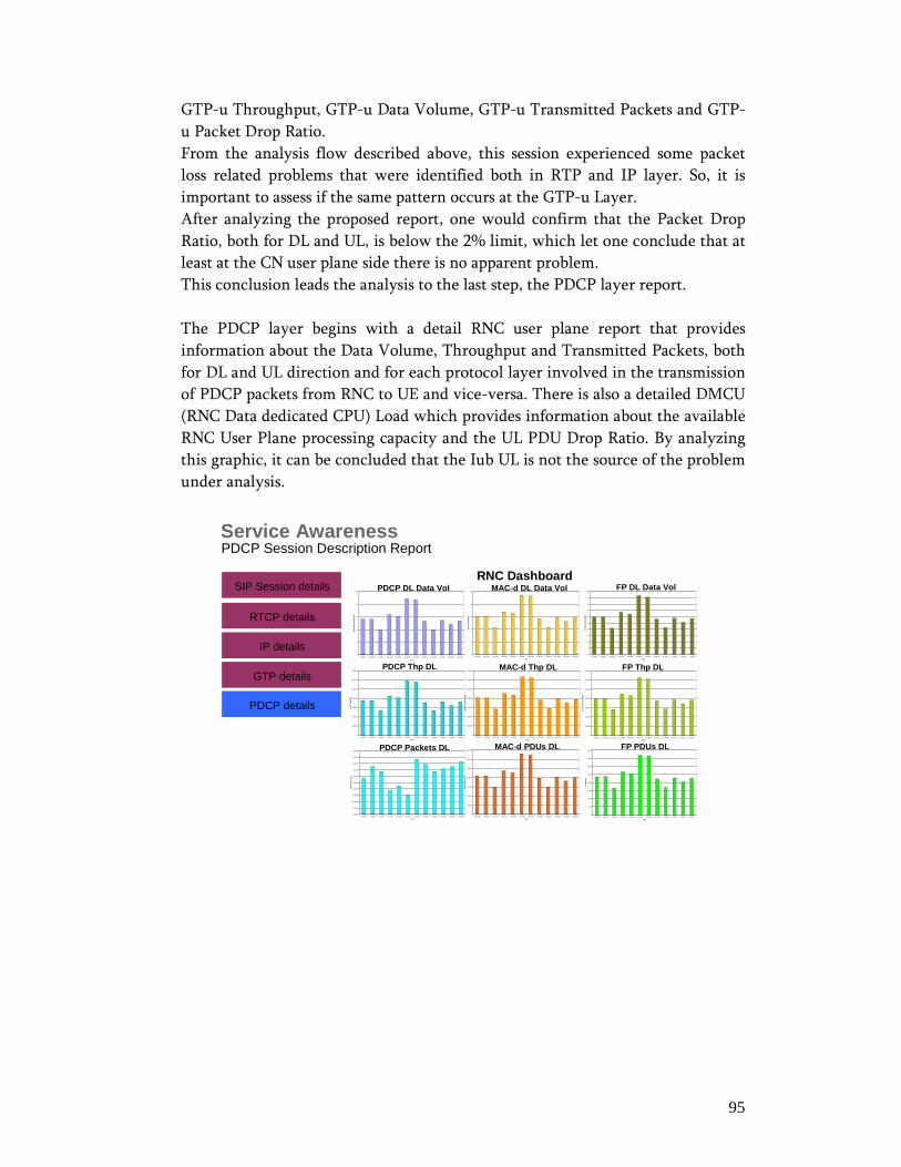
95
GTP-u Throughput, GTP-u Data Volume, GTP-u Transmitted Packets and GTP-
u Packet Drop Ratio.
From the analysis flow described above, this session experienced some packet
loss related problems that were identified both in RTP and IP layer. So, it is
important to assess if the same pattern occurs at the GTP-u Layer.
After analyzing the proposed report, one would confirm that the Packet Drop
Ratio, both for DL and UL, is below the 2% limit, which let one conclude that at
least at the CN user plane side there is no apparent problem.
This conclusion leads the analysis to the last step, the PDCP layer report.
The PDCP layer begins with a detail RNC user plane report that provides
information about the Data Volume, Throughput and Transmitted Packets, both
for DL and UL direction and for each protocol layer involved in the transmission
of PDCP packets from RNC to UE and vice-versa. There is also a detailed DMCU
(RNC Data dedicated CPU) Load which provides information about the available
RNC User Plane processing capacity and the UL PDU Drop Ratio. By analyzing
this graphic, it can be concluded that the Iub UL is not the source of the problem
under analysis.
Service AwarenessPDCP Session Description Report
SIP Session details
RTCP details
IP details
GTP details
PDCP details
0
5
10
15
20
25
16:00:00 16:05:00 16:10:00 16:15:00 16:20:00 16:25:00 16:30:00 16:35:00 16:40:00 16:45:00 16:50:00 16:55:00
Time
PD
CP
Da
ta V
olu
me
(M
B)
PDCP DL Data Vol
300000
301000
302000
303000
304000
305000
306000
307000
308000
309000
310000
16:00:00 16:05:00 16:10:00 16:15:00 16:20:00 16:25:00 16:30:00 16:35:00 16:40:00 16:45:00 16:50:00 16:55:00
Time
PD
CP
Pa
cke
t (N
r)
PDCP Packets DL
0
5
10
15
20
25
16:00:00 16:05:00 16:10:00 16:15:00 16:20:00 16:25:00 16:30:00 16:35:00 16:40:00 16:45:00 16:50:00 16:55:00
Time
MA
C-d
Vol
um
e (M
B)
MAC-d DL Data Vol
0
100000
200000
300000
400000
500000
600000
700000
16:00:00 16:05:00 16:10:00 16:15:00 16:20:00 16:25:00 16:30:00 16:35:00 16:40:00 16:45:00 16:50:00 16:55:00
Time
PD
CP
Thp
(MB
)
PDCP Thp DL
0
100000
200000
300000
400000
500000
600000
700000
16:00:00 16:05:00 16:10:00 16:15:00 16:20:00 16:25:00 16:30:00 16:35:00 16:40:00 16:45:00 16:50:00 16:55:00
Time
MA
C-d
Thp
DL
(Mb
ps)
MAC-d Thp DL
0
50000
100000
150000
200000
250000
300000
350000
16:00:00 16:05:00 16:10:00 16:15:00 16:20:00 16:25:00 16:30:00 16:35:00 16:40:00 16:45:00 16:50:00 16:55:00
Time
MA
C-d
PD
U (N
r)
MAC-d PDUs DL
RNC Dashboard
0
5
10
15
20
25
30
35
40
45
50
16:00:00 16:05:00 16:10:00 16:15:00 16:20:00 16:25:00 16:30:00 16:35:00 16:40:00 16:45:00 16:50:00 16:55:00
Time
FP
Da
ta V
olum
e (M
B)
FP DL Data Vol
0
200000
400000
600000
800000
1000000
1200000
1400000
16:00:00 16:05:00 16:10:00 16:15:00 16:20:00 16:25:00 16:30:00 16:35:00 16:40:00 16:45:00 16:50:00 16:55:00
Time
FP
Thr
oug
hput
(Mb
ps)
FP Thp DL
0
5000
10000
15000
20000
25000
30000
35000
40000
16:00:00 16:05:00 16:10:00 16:15:00 16:20:00 16:25:00 16:30:00 16:35:00 16:40:00 16:45:00 16:50:00 16:55:00
Time
FP P
DU
(Nr)
FP PDUs DL
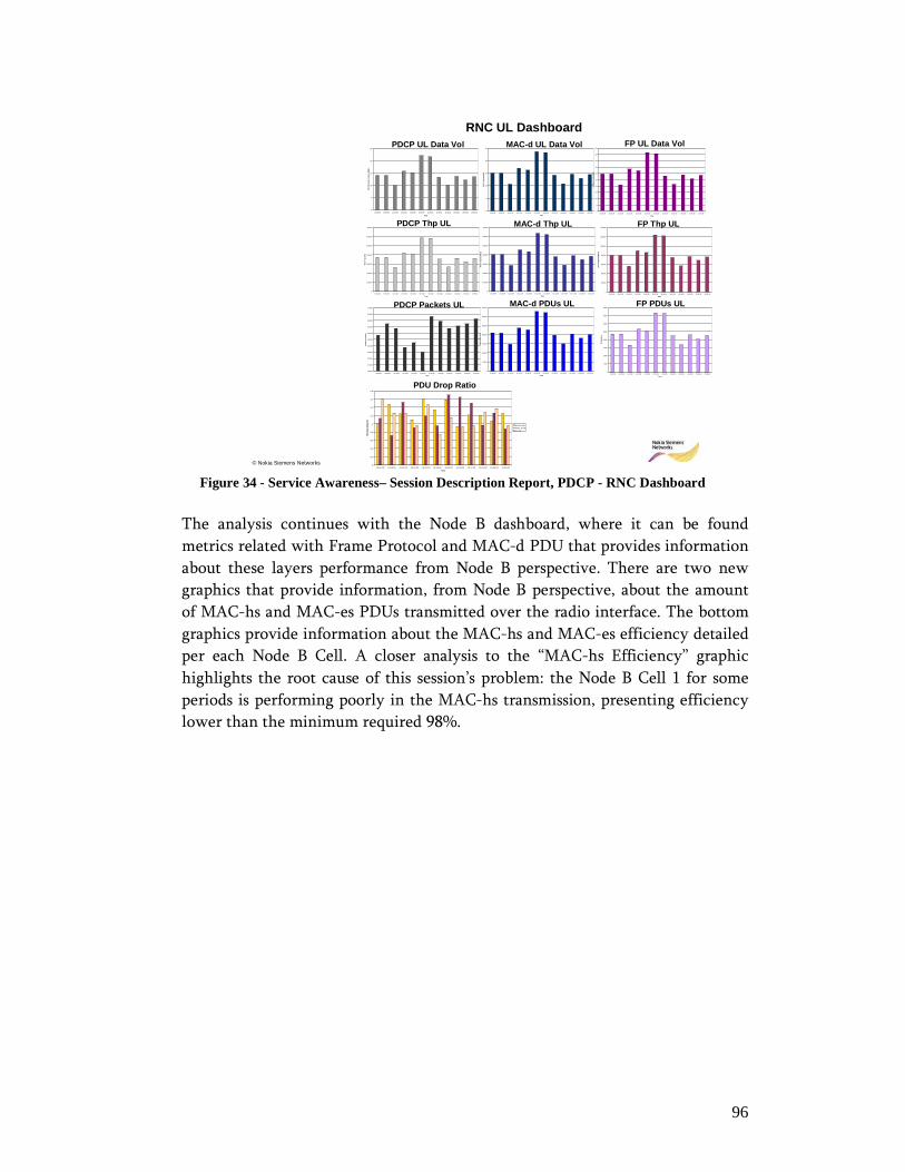
96
© Nokia Siemens Networks
0
5
10
15
20
25
16:00:00 16:05:00 16:10:00 16:15:00 16:20:00 16:25:00 16:30:00 16:35:00 16:40:00 16:45:00 16:50:00 16:55:00
Time
PD
CP
Dat
a V
olu
me
(MB
)
PDCP UL Data Vol
300000
301000
302000
303000
304000
305000
306000
307000
308000
309000
310000
16:00:00 16:05:00 16:10:00 16:15:00 16:20:00 16:25:00 16:30:00 16:35:00 16:40:00 16:45:00 16:50:00 16:55:00
Time
PD
CP
Pa
cke
t (N
r)
PDCP Packets UL
0
5
10
15
20
25
16:00:00 16:05:00 16:10:00 16:15:00 16:20:00 16:25:00 16:30:00 16:35:00 16:40:00 16:45:00 16:50:00 16:55:00
Time
MA
C-d
Vol
um
e (M
B)
MAC-d UL Data Vol
0
100000
200000
300000
400000
500000
600000
700000
16:00:00 16:05:00 16:10:00 16:15:00 16:20:00 16:25:00 16:30:00 16:35:00 16:40:00 16:45:00 16:50:00 16:55:00
Time
PD
CP
Thp
(M
B)
PDCP Thp UL
0
100000
200000
300000
400000
500000
600000
700000
16:00:00 16:05:00 16:10:00 16:15:00 16:20:00 16:25:00 16:30:00 16:35:00 16:40:00 16:45:00 16:50:00 16:55:00
Time
MA
C-d
Thp
DL
(Mbp
s)
MAC-d Thp UL
0
50000
100000
150000
200000
250000
300000
350000
16:00:00 16:05:00 16:10:00 16:15:00 16:20:00 16:25:00 16:30:00 16:35:00 16:40:00 16:45:00 16:50:00 16:55:00
Time
MA
C-d
PD
U (
Nr)
MAC-d PDUs UL
RNC UL Dashboard
0
5
10
15
20
25
30
35
40
45
50
16:00:00 16:05:00 16:10:00 16:15:00 16:20:00 16:25:00 16:30:00 16:35:00 16:40:00 16:45:00 16:50:00 16:55:00
Time
FP
Da
ta V
olum
e (M
B)
FP UL Data Vol
0
200000
400000
600000
800000
1000000
1200000
1400000
16:00:00 16:05:00 16:10:00 16:15:00 16:20:00 16:25:00 16:30:00 16:35:00 16:40:00 16:45:00 16:50:00 16:55:00
Time
FP T
hro
ughp
ut (
Mbp
s)
FP Thp UL
0
5000
10000
15000
20000
25000
30000
35000
40000
16:00:00 16:05:00 16:10:00 16:15:00 16:20:00 16:25:00 16:30:00 16:35:00 16:40:00 16:45:00 16:50:00 16:55:00
Time
FP P
DU
(Nr)
FP PDUs UL
0
0,2
0,4
0,6
0,8
1
1,2
1,4
1,6
1,8
16:00:00 16:05:00 16:10:00 16:15:00 16:20:00 16:25:00 16:30:00 16:35:00 16:40:00 16:45:00 16:50:00 16:55:00
Time
PD
U D
rop
Ratio
(%)
PDCP DR
MAC-d DR
FP DR
PDU Drop Ratio
Figure 34 - Service Awareness– Session Description Report, PDCP - RNC Dashboard
The analysis continues with the Node B dashboard, where it can be found
metrics related with Frame Protocol and MAC-d PDU that provides information
about these layers performance from Node B perspective. There are two new
graphics that provide information, from Node B perspective, about the amount
of MAC-hs and MAC-es PDUs transmitted over the radio interface. The bottom
graphics provide information about the MAC-hs and MAC-es efficiency detailed
per each Node B Cell. A closer analysis to the “MAC-hs Efficiency” graphic
highlights the root cause of this session’s problem: the Node B Cell 1 for some
periods is performing poorly in the MAC-hs transmission, presenting efficiency
lower than the minimum required 98%.

97
© Nokia Siemens Networks
Service AwarenessPDCP Session Description Report
SIP Session details
RTCP details
IP details
GTP details
PDCP details
Node B Dashboard
0
5000
10000
15000
20000
25000
30000
35000
40000
16:00:00 16:05:00 16:10:00 16:15:00 16:20:00 16:25:00 16:30:00 16:35:00 16:40:00 16:45:00 16:50:00 16:55:00
Time
FP P
DU
(Nr)
FP PDUs UL
0
5000
10000
15000
20000
25000
30000
35000
40000
16:00:00 16:05:00 16:10:00 16:15:00 16:20:00 16:25:00 16:30:00 16:35:00 16:40:00 16:45:00 16:50:00 16:55:00
Time
FP P
DU
(Nr)
FP PDUs DL
0
50000
100000
150000
200000
250000
300000
350000
16:00:00 16:05:00 16:10:00 16:15:00 16:20:00 16:25:00 16:30:00 16:35:00 16:40:00 16:45:00 16:50:00 16:55:00
Time
MA
C-d
PD
U (
Nr)
MAC-d PDUs UL
0
50000
100000
150000
200000
250000
300000
350000
16:00:00 16:05:00 16:10:00 16:15:00 16:20:00 16:25:00 16:30:00 16:35:00 16:40:00 16:45:00 16:50:00 16:55:00
Time
MA
C-d
PD
U (
Nr)
MAC-d PDUs DL
0
50000
100000
150000
200000
250000
300000
350000
16:00:00 16:05:00 16:10:00 16:15:00 16:20:00 16:25:00 16:30:00 16:35:00 16:40:00 16:45:00 16:50:00 16:55:00
Time
MA
C-d
PD
U (
Nr)
MAC-hs PDUs
0
50000
100000
150000
200000
250000
300000
350000
16:00:00 16:05:00 16:10:00 16:15:00 16:20:00 16:25:00 16:30:00 16:35:00 16:40:00 16:45:00 16:50:00 16:55:00
Time
MA
C-d
PD
U (
Nr)
MAC-es PDUs
96
96,5
97
97,5
98
98,5
99
99,5
100
16:00:00 16:05:00 16:10:00 16:15:00 16:20:00 16:25:00 16:30:00 16:35:00 16:40:00 16:45:00 16:50:00 16:55:00
Time
MA
C-h
s E
ffici
ency
(%)
MAC-hs Efficiency
98
98,2
98,4
98,6
98,8
99
99,2
99,4
99,6
99,8
16:00:00 16:05:00 16:10:00 16:15:00 16:20:00 16:25:00 16:30:00 16:35:00 16:40:00 16:45:00 16:50:00 16:55:00
Time
MA
C-e
s E
ffici
ency
(%)
MAC-es Efficiency
Figure 35 - Service Awareness– Session Description Report, PDCP – Node B Dashboard
The analysis of the Cell Dashboard confirms that a problem, related with MAC-
hs efficiency, definitely exists in Cell 1 and analyzing in detail the “MAC-hs
BLER, per Cause” graphic, it can be seen that the “Timer T1” cause is
significantly contributing for such poor performance. The conclusion to take
from this analysis flow is that the session serving cell HSDPA parameters has to
be optimized, mainly T1 Timer parameter, has its current setting is affecting the
VoIP service delivery.
This analysis flow may have other innumerous alternative analysis paths. In this
case it was shown that the problem first identified was the packet loss ratio being
higher than 2%, and the conclusion is that it was caused by a radio interface
related bottleneck. However, this flow concept can efficiently be used to track
other issues like delay, jitter, distortion, voice signal power or noise level effects.
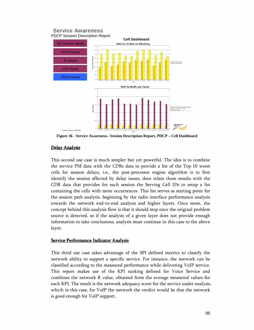
98
© Nokia Siemens Networks
Service AwarenessPDCP Session Description Report
SIP Session details
RTCP details
IP details
GTP details
PDCP details
Cell Dashboard
96
96,5
97
97,5
98
98,5
99
99,5
100
16:00:00 16:05:00 16:10:00 16:15:00 16:20:00 16:25:00 16:30:00 16:35:00 16:40:00 16:45:00 16:50:00 16:55:00
Time
MAC-hs an
d MAC-e
s Efficien
cy (%
)
MAC-hs Efficiency
MAC-es Efficiency
MAC-hs Vs MAC-es Efficiency
0
0,5
1
1,5
2
2,5
16:00:00 16:05:00 16:10:00 16:15:00 16:20:00 16:25:00 16:30:00 16:35:00 16:40:00 16:45:00 16:50:00 16:55:00
Time
MAC-h
s BLE
R (%
)
MAC-hs BLER, Max Nbr Retrans
MAC-hs BLER, T1 Timer
MAC-hs, Other
MAC-hs BLER, per Cause
Figure 36 - Service Awareness– Session Description Report, PDCP – Cell Dashboard
Delay AnalysisDelay AnalysisDelay AnalysisDelay Analysis
This second use case is much simpler but yet powerful. The idea is to combine
the service PM data with the CDRs data to provide a list of the Top-10 worst
cells for session delays, i.e., the post-processor engine algorithm is to first
identify the session affected by delay issues, then relate these results with the
CDR data that provides for each session the Serving Cell IDs to setup a list
containing the cells with more occurrences. This list serves as starting point for
the session path analysis, beginning by the radio interface performance analysis
towards the network end-to-end analysis and higher layers. Once more, the
concept behind this analysis flow is that it should stop once the original problem
source is detected, so if the analysis of a given layer does not provide enough
information to take conclusions, analysis must continue in this case to the above
layer.
Service Performance Indicator AnalysisService Performance Indicator AnalysisService Performance Indicator AnalysisService Performance Indicator Analysis
This third use case takes advantage of the SPI defined metrics to classify the
network ability to support a specific service. For instance, the network can be
classified according to the measured performance while delivering VoIP service.
This report makes use of the KPI ranking defined for Voice Service and
combines the network R value, obtained from the average measured values for
each KPI. The result is the network adequacy score for the service under analysis,
which in this case, for VoIP the network the verdict would be that the network
is good enough for VoIP support.

99
© Nokia Siemens Networks
Service Performance Evaluation
131718TK
251Bit Rates
212Waiting Time
123Jitter
233Discard Rate
344Reliability
325E2EDelay
Browsing:
Video:Voice:
KPRV By Type Of ServiceKPI:
VoIP report
>100<90>10>2D> 6000
[10;100][90;99][1;10][D;2D][300;600]1
[1;10][99.9;99][0.1;1][0.8D;D][150;300]2
[0.1;1][99.9;99.999][0.01;0.1][0.5D;0.8D][100;150]3
[0.001;0.1][99.99;99.9999][0.001;0.01][0.1D;0.5D][50;100]4
<0.01>99.999<0.001<0.1xDelay<505
WT (s)Reliability (%)Discard Rate (%)
Jitter (ms)Delay(ms)
R
SPIvoice Network Score=3,7
E2EDelay=5*3
Reliability= 4*5
Discard Rate= 3*5
Jitter= 3*3
Waiting Time= 2*2
Bit Rates= 1*5
TK=18
SPI=3,7 -> Network is good enough for VoIP delivery
Figure 37 - Service Performance Evaluation - Network Classification for VoIP delivery
100
3333....8888.... ConclusionConclusionConclusionConclusion
This chapter introduces the fundamental concepts developed in this work. It
describes in detail an architectural proposal to cope with Performance
Management system requirements. This architecture is divided in three
fundamental parts: Network infrastructure composed by all system NEs; Element
Manager responsible for managing the NEs and collecting the network PM data;
Reporting tool responsible for data modeling and aggregation, statistical post-
processing and data visualization engine. This architecture provides all the
mechanisms and interfaces to allow PM data management end-to-end
functionality, from the NE until the report generation for post performance
analysis.
This chapter further details the adopted information model and its components
described in network and service model metadata. Metadata is composed by
Configuration Management (CM) information, which describes the network
elements configuration detailing the topology, hierarchy, attributes and
characteristics. CM information is stored in Object Class (OC) tree, where each
object instance describes a network entity. Performance Management (PM)
information is composed by measurements and counters that provide actual
insight about network and service behavior. Each measurement is related with
an OC and is composed by a set of counters that can describe protocols or
procedures performance, hardware resource usage, processor load, etc. Fault
Management (FM) information provides indications about system faults that can
be of hardware or software type and are categorized by severity.
This chapter also describes the several data sources that are available both at
network and service layers and enable the monitoring capabilities. These data
sources are detailed per network sub-system, and it is also explained the kind of
statistics that can be retrieved and their purpose. There are several data sources
used in this work: PM data for RAN and CN; CDR data for session context
description; and Deep Packet Inspection statistics that provide IP-based
performance.
ETL process is also mentioned in this chapter. This is a very important process in
the overall proposed Performance Management system, since it is responsible for
implementing all the data collection, conversion and storage procedures, a cycle
which has a high performance demand. There is often the requirement for ETL
process to cope with a period of fifteen minutes, meaning that in this period the
system must collect, convert and store thousand of PM data Mbytes. Extraction
process is responsible to collect thousands of PM files from the entire network,
using different collection mechanisms such as FTP, CORBA, etc. The
Transformation process is responsible to convert different types and data formats
into a single integrated and model coherent data-warehouse. The transformation
process must have the ability to convert from different type of files and formats
like XML, ASCII and often has even to handle with proprietary formats. Loading

101
is the process responsible for storing all the data contained in the PM data
converted in to the data-warehouse defined model.
This work proposes a simplified model for both network and service PM data,
which is used to define and create the database structure that is used to load the
CM, PM and FM data collected from all the identified sources.
The KPIs section provides information about the heart of this project, defines the
fundamental performance indicators that must be used to establish relations in
the identified layers and the impact that they have in each other. There are
proposed KPIs for Network and Service layer, organized per system functional
part: (ex. RAN, CN, Service, etc.); and per functional logic: Control Plane and
User Plane.
Finally, this chapter describes some of the most important reporting use cases
designed within this work. This is the part where the relation between layers is
described and the analysis logic behind each report proposal. The proposed
reports cover both reactive and proactive monitoring.

102
4444.... SimulationSimulationSimulationSimulation
This chapter presents the simulation related information. Section 4.1 introduces the
simulation objectives and describes the simulation environment setup. Section 4.2
presents the obtained simulation results. Section 4.3 presents the simulation result
analysis and conclusions.
4444....1111.... Simulation EnvironmentSimulation EnvironmentSimulation EnvironmentSimulation Environment
The simulation work within this thesis served to assess the VoIP over HSPA
network as a feasible scenario, by validating the service performance metrics.
Furthermore, there is also the objective to compare the HSPA performance
against UMTS R99.
The OpNet was chosen as the simulation tool to create a 3GPP Packet Switched
network containing both R99 and HSPA elements and run the different
simulation scenarios, comparing the results obtained from each other. Three
simulation scenarios were implemented, representing different periods of the
week with different traffic loads and usage.
Across the different scenarios the network topology is the same with varying
traffic model.
The deployed simulation network model is composed by the following elements:
• 1 GGSN;
• 1 SGSN;
• 4 RNCs;
• 3 Node B HSPA capable;
• 1 Rel99 Node B;
• 22 HSPA capable UEs;
• 6 Rel99 UEs.

103
Figure 38 - OpNet – Modeled HSPA Simulation network
Since the OpNet does not offer any default HSPA model or NE, it was necessary
to create the model that replicates HSDPA and HSUPA features, and both UEs
and Node Bs were changed.
The changes performed to the Node Bs in order to enable HSDPA features can be
seen in the Fig. 37.
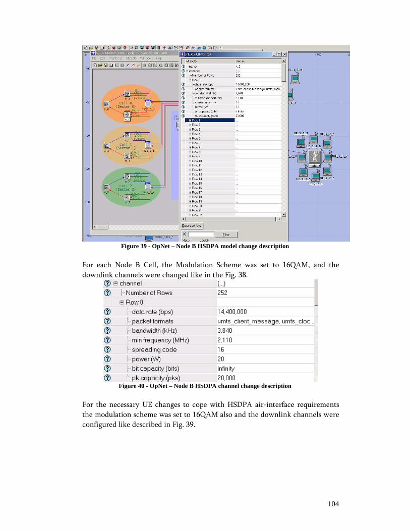
104
Figure 39 - OpNet – Node B HSDPA model change description
For each Node B Cell, the Modulation Scheme was set to 16QAM, and the
downlink channels were changed like in the Fig. 38.
Figure 40 - OpNet – Node B HSDPA channel change description
For the necessary UE changes to cope with HSDPA air-interface requirements
the modulation scheme was set to 16QAM also and the downlink channels were
configured like described in Fig. 39.

105
Figure 41 - OpNet – UE HSDPA change description
For the HSUPA model, it was also necessary to perform some changes in the
Node B and UE uplink channel and modulation schemes.
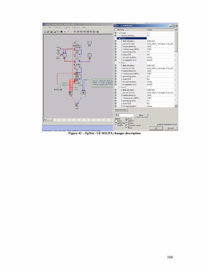
106
Figure 42 – OpNet - UE HSUPA changes description
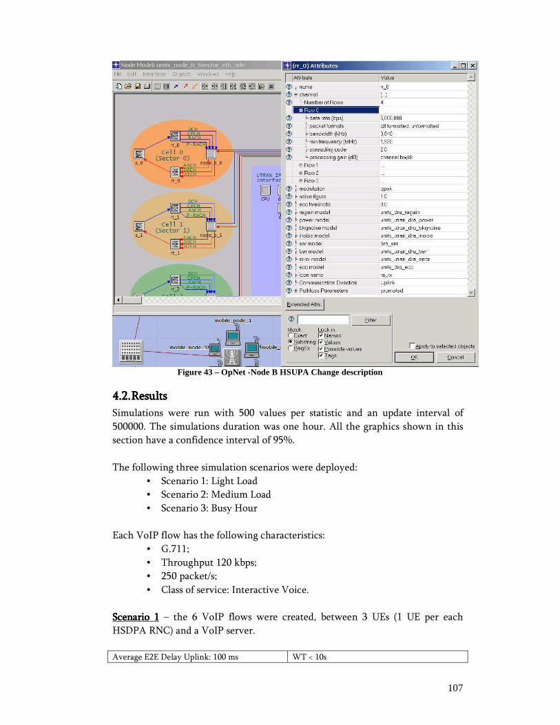
107
Figure 43 – OpNet -Node B HSUPA Change description
4444....2222.... ResultsResultsResultsResults
Simulations were run with 500 values per statistic and an update interval of
500000. The simulations duration was one hour. All the graphics shown in this
section have a confidence interval of 95%.
The following three simulation scenarios were deployed:
• Scenario 1: Light Load
• Scenario 2: Medium Load
• Scenario 3: Busy Hour
Each VoIP flow has the following characteristics:
• G.711;
• Throughput 120 kbps;
• 250 packet/s;
• Class of service: Interactive Voice.
Scenario 1Scenario 1Scenario 1Scenario 1 – the 6 VoIP flows were created, between 3 UEs (1 UE per each
HSDPA RNC) and a VoIP server.
Average E2E Delay Uplink: 100 ms WT < 10s
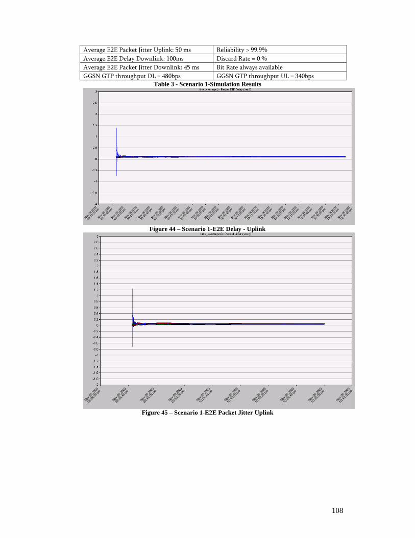
108
Average E2E Packet Jitter Uplink: 50 ms Reliability > 99.9%
Average E2E Delay Downlink: 100ms Discard Rate = 0 %
Average E2E Packet Jitter Downlink: 45 ms Bit Rate always available
GGSN GTP throughput DL = 480bps GGSN GTP throughput UL = 340bps
Table 3 - Scenario 1-Simulation Results
Figure 44 – Scenario 1-E2E Delay - Uplink
Figure 45 – Scenario 1-E2E Packet Jitter Uplink
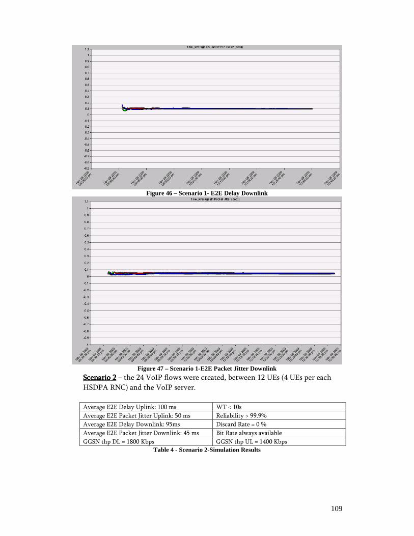
109
Figure 46 – Scenario 1- E2E Delay Downlink
Figure 47 – Scenario 1-E2E Packet Jitter Downlink
Scenario Scenario Scenario Scenario 2222 – the 24 VoIP flows were created, between 12 UEs (4 UEs per each
HSDPA RNC) and the VoIP server.
Average E2E Delay Uplink: 100 ms WT < 10s
Average E2E Packet Jitter Uplink: 50 ms Reliability > 99.9%
Average E2E Delay Downlink: 95ms Discard Rate = 0 %
Average E2E Packet Jitter Downlink: 45 ms Bit Rate always available
GGSN thp DL = 1800 Kbps GGSN thp UL = 1400 Kbps
Table 4 - Scenario 2-Simulation Results

110
Figure 48 - Scenario 2-E2E Delay Uplink
Figure 49- Scenario 2-E2E Packet Jitter Uplink
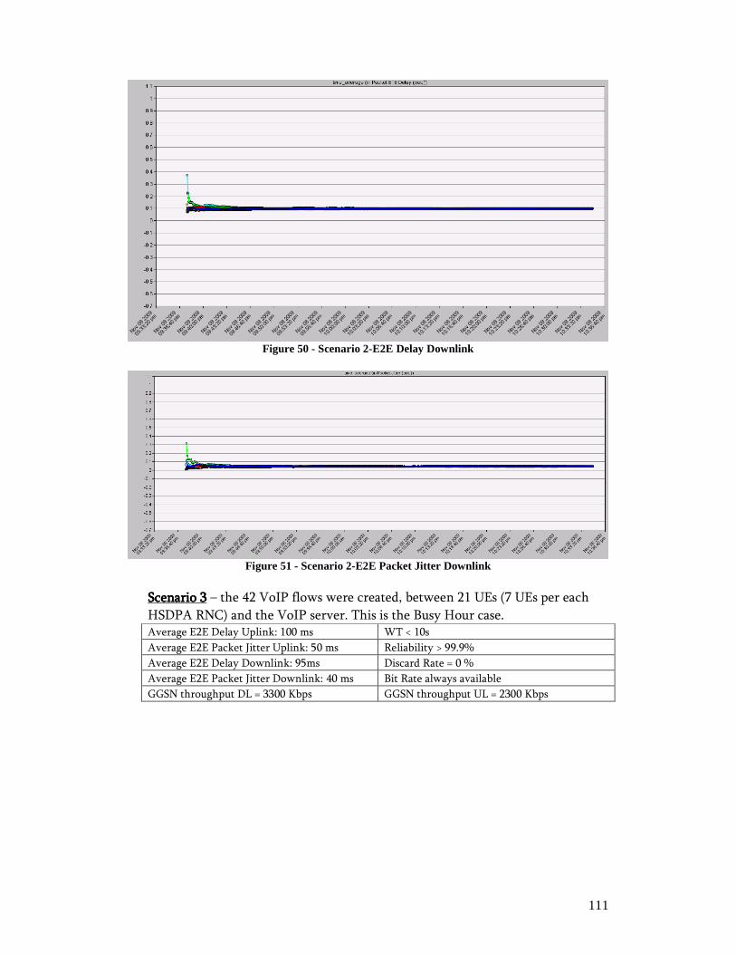
111
Figure 50 - Scenario 2-E2E Delay Downlink
Figure 51 - Scenario 2-E2E Packet Jitter Downlink
Scenario Scenario Scenario Scenario 3333 – the 42 VoIP flows were created, between 21 UEs (7 UEs per each
HSDPA RNC) and the VoIP server. This is the Busy Hour case. Average E2E Delay Uplink: 100 ms WT < 10s
Average E2E Packet Jitter Uplink: 50 ms Reliability > 99.9%
Average E2E Delay Downlink: 95ms Discard Rate = 0 %
Average E2E Packet Jitter Downlink: 40 ms Bit Rate always available
GGSN throughput DL = 3300 Kbps GGSN throughput UL = 2300 Kbps
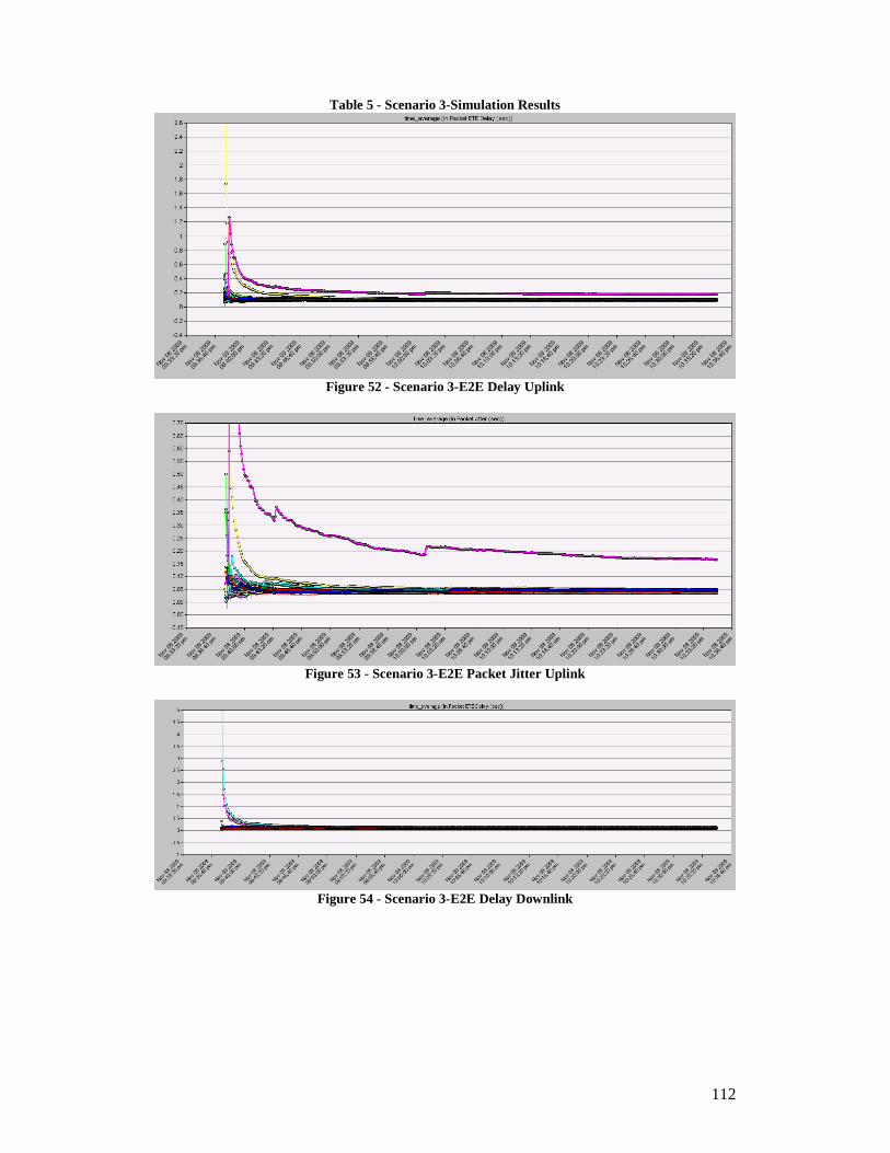
112
Table 5 - Scenario 3-Simulation Results
Figure 52 - Scenario 3-E2E Delay Uplink
Figure 53 - Scenario 3-E2E Packet Jitter Uplink
Figure 54 - Scenario 3-E2E Delay Downlink
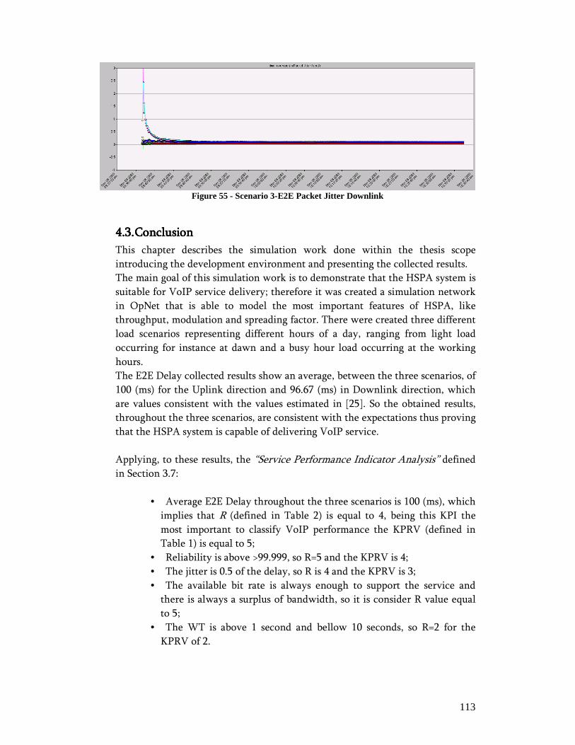
113
Figure 55 - Scenario 3-E2E Packet Jitter Downlink
4444....3333.... ConclusionConclusionConclusionConclusion
This chapter describes the simulation work done within the thesis scope
introducing the development environment and presenting the collected results.
The main goal of this simulation work is to demonstrate that the HSPA system is
suitable for VoIP service delivery; therefore it was created a simulation network
in OpNet that is able to model the most important features of HSPA, like
throughput, modulation and spreading factor. There were created three different
load scenarios representing different hours of a day, ranging from light load
occurring for instance at dawn and a busy hour load occurring at the working
hours.
The E2E Delay collected results show an average, between the three scenarios, of
100 (ms) for the Uplink direction and 96.67 (ms) in Downlink direction, which
are values consistent with the values estimated in [25]. So the obtained results,
throughout the three scenarios, are consistent with the expectations thus proving
that the HSPA system is capable of delivering VoIP service.
Applying, to these results, the “Service Performance Indicator Analysis” defined
in Section 3.7:
• Average E2E Delay throughout the three scenarios is 100 (ms), which
implies that R (defined in Table 2) is equal to 4, being this KPI the
most important to classify VoIP performance the KPRV (defined in
Table 1) is equal to 5;
• Reliability is above >99.999, so R=5 and the KPRV is 4;
• The jitter is 0.5 of the delay, so R is 4 and the KPRV is 3;
• The available bit rate is always enough to support the service and
there is always a surplus of bandwidth, so it is consider R value equal
to 5;
• The WT is above 1 second and bellow 10 seconds, so R=2 for the
KPRV of 2.

114
The HSPA network achieves a score of 3.94 out 5 while delivering the VoIP
service.
The results obtained in this chapter also serve as proof of concept for the work
developed in this thesis, by classifying the underlying network performance
according to the delivered service demands. Due to the fact that this approach is
technological agnostic it can be used to relate network performance with service
behavior for every kind of underlying packet network, fixed or mobile, and be
even extended to analyze different types of IP-based services.
The cross-layer approach proposed in this Thesis divides the analysis scope into
two inter-dependent layers: Network layer and IP-based service layer; it is also
validated by these results thus relating the network performance with service
delivery QoS and providing mechanisms to classify the adequacy of a specific
network to deliver a specific service, perform troubleshooting, forecast analysis,
predict faults and the need for capacity improvements.
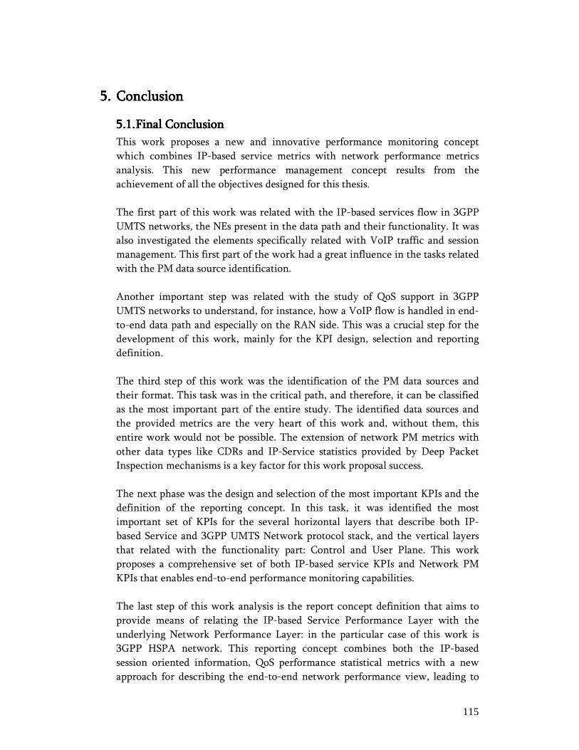
115
5555.... ConclusionConclusionConclusionConclusion
5555....1111.... Final ConclusionFinal ConclusionFinal ConclusionFinal Conclusion
This work proposes a new and innovative performance monitoring concept
which combines IP-based service metrics with network performance metrics
analysis. This new performance management concept results from the
achievement of all the objectives designed for this thesis.
The first part of this work was related with the IP-based services flow in 3GPP
UMTS networks, the NEs present in the data path and their functionality. It was
also investigated the elements specifically related with VoIP traffic and session
management. This first part of the work had a great influence in the tasks related
with the PM data source identification.
Another important step was related with the study of QoS support in 3GPP
UMTS networks to understand, for instance, how a VoIP flow is handled in end-
to-end data path and especially on the RAN side. This was a crucial step for the
development of this work, mainly for the KPI design, selection and reporting
definition.
The third step of this work was the identification of the PM data sources and
their format. This task was in the critical path, and therefore, it can be classified
as the most important part of the entire study. The identified data sources and
the provided metrics are the very heart of this work and, without them, this
entire work would not be possible. The extension of network PM metrics with
other data types like CDRs and IP-Service statistics provided by Deep Packet
Inspection mechanisms is a key factor for this work proposal success.
The next phase was the design and selection of the most important KPIs and the
definition of the reporting concept. In this task, it was identified the most
important set of KPIs for the several horizontal layers that describe both IP-
based Service and 3GPP UMTS Network protocol stack, and the vertical layers
that related with the functionality part: Control and User Plane. This work
proposes a comprehensive set of both IP-based service KPIs and Network PM
KPIs that enables end-to-end performance monitoring capabilities.
The last step of this work analysis is the report concept definition that aims to
provide means of relating the IP-based Service Performance Layer with the
underlying Network Performance Layer: in the particular case of this work is
3GPP HSPA network. This reporting concept combines both the IP-based
session oriented information, QoS performance statistical metrics with a new
approach for describing the end-to-end network performance view, leading to

116
an innovative troubleshooting, optimization and planning tool proposal. This
new reporting concept will be integrated in the Nokia Siemens Network solution
portfolio.
The new performance monitoring concepts introduced by this work are a very
important step towards the All IP Mobile Network Performance Management
area, which provides the means and tools for Network Operators and Service
Providers monitor the performance of their sub-systems and also the SLA
agreements. This will allow setting a new trend in Operational Support Systems,
Performance Management and Service Assurance solutions.
This work also provides some simulation results which show that the VoIP over
HSPA networks is a feasible scenario, thus proving the effectiveness of this work,
since this will become a frequent scenario in the near future.
5555....2222.... Future WorkFuture WorkFuture WorkFuture Work
As future work, the performance monitoring concept introduced in this thesis
can be extended, mainly to detail the support of mobility scenarios, both
geographical mobility and inter-RAT mobility.
Moreover, since the objective of this work was the proposal of a generic
performance monitoring concept, this work can also be extended to support
other network technologies and analysis scenarios, such as multi-technology
reports.
Finally, the proposed report use cases can be implemented and tested within a
real-network premise, in order to be productized and integrated in the Nokia
Siemens Network portfolio.
117
ReferencesReferencesReferencesReferences
[1] International Engineering Consortium: Operations Support Systems (OSSs) -
http://www.iec.org/online/tutorials/oss/index.asp
[2] UMTS Networks – Architecture, Mobility and Services. Heikki Kaaranen, Ari
Ahtiainen, Lauri Laitinen, Siamak Naghian, Valtteri Niemi
[3] ISO/IEC 7498-4 Information processing systems – Open Systems Interconnection
– Basic Reference Model – Part 4: Management Framework
[4] ISO/IEC 9596-1 Information technology - Open Systems Interconnection --
Common management information protocol - Part 1: Specification
[5] RFC1157 - Simple Network Management Protocol (SNMP)
[6] RFC1052 - IAB Recommendations for the Development of Internet Network
Management Standards
[7] M.3000: Overview of TMN Recommendations
[8] 3GPP TS 23.002 – Network Architecture
[9] 3GPP TS 25.331 – Radio Resource Control (RRC); Protocol specification
[10] 3GPP TS 24.008 – Mobile radio interface Layer 3 specification; Core network
protocols
[11] 3GPP TS 25.413 – UTRAN Iu interface Radio Access Network Application Part
(RANAP) signalling
[12] 3GPP TS 25.423 – UTRAN Iur interface Radio Network Subsystem Application
Part (RNSAP) signalling
[13] 3GPP TS 25.211 – Physical channels and mapping of transport channels onto
physical channels (FDD)
[14] 3GPP TS 25.308 – High Speed Downlink Packet Access (HSDPA); Overall
description.
[15] 3GPP TS 25.309 – FDD enhanced uplink; Overall description;
[16] 3GPP TS 36.300 – Evolved Universal Terrestrial Radio Access (E-UTRA) and
Evolved Universal Terrestrial Radio Access Network (E-UTRAN); Overall
description;
[17] in http://www.ccpu.com/products/trillium/3ghspa.html
[18] in dpacket.org – www.dpacket.org
[19] D. Malas, “SIP End-to-End Performance Metrics”, IETF Draft, PMOL WG, June
25, 2008
[20] RFC 3550 - RTP: A Transport Protocol for Real-Time Applications
[21] RTCP HR - High Resolution VoIP Metrics Report Blocks draft-ietf-avt-rtcphr-
03.txt, February 25, 2008
[22] The Data Warehouse ETL Toolkit – Practical Techniques for Extracting,
Cleaning, Conforming, and Delivering Data, Ralph Kimball, Joe Caserta
[23] Miguel Almeida, Rui Inácio, Susana Sargento, “Cross Layer Design Approach for
Performance Evaluation of Multimedia Contents”
[24] WCDMA for UMTS – HSPA Evolution and LTE 4th Edition, Harri Holma, Anti

118
Toskala
[25] HSDPA/HSUPA for UMTS, Harri Holma, Anti Toskala
[26] WCDMA for UMTS 3rd Edition, Harri Holma, Anti Toskala
[27] UMTS Performance Measurement - A Practical Guide to KPIs for the UTRAN
Environment, Ralf Kreher
Recommended