Seismic fragility curves for structures using non-parametric
representations
C. Mai1, K. Konakli1, and B. Sudret1
1Chair of Risk, Safety and Uncertainty Quantification,
ETH Zurich, Stefano-Franscini-Platz 5, 8093 Zurich, Switzerland
Abstract
Fragility curves are commonly used in civil engineering to assess the vulnerability of struc-
tures to earthquakes. The probability of failure associated with a prescribed criterion (e.g. the
maximal inter-storey drift of a building exceeding a certain threshold) is represented as a func-
tion of the intensity of the earthquake ground motion (e.g. peak ground acceleration or spectral
acceleration). The classical approach relies on assuming a lognormal shape of the fragility curves;
it is thus parametric. In this paper, we introduce two non-parametric approaches to establish
the fragility curves without employing the above assumption, namely binned Monte Carlo sim-
ulation and kernel density estimation. As an illustration, we compute the fragility curves for a
three-storey steel frame using a large number of synthetic ground motions. The curves obtained
with the non-parametric approaches are compared with respective curves based on the lognormal
assumption. A similar comparison is presented for a case when a limited number of recorded
ground motions is available. It is found that the accuracy of the lognormal curves depends on the
ground motion intensity measure, the failure criterion and most importantly, on the employed
method for estimating the parameters of the lognormal shape.
Keywords: earthquake engineering – fragility curves – lognormal assumption – non-parametric
approach – kernel density estimation – epistemic uncertainty
1 Introduction
The severe socio-economic consequences of several recent earthquakes highlight the need for
proper seismic risk assessment as a basis for efficient decision making on mitigation actions
1
arX
iv:1
704.
0387
6v1
[st
at.A
P] 1
2 A
pr 2
017

and disaster planning. To this end, the probabilistic performance-based earthquake engineering
(PBEE) framework has been developed, which allows explicit evaluation of performance measures
that serve as decision variables (DV) (e.g. monetary losses, casualties, downtime) accounting for
the prevailing uncertainties (e.g. ground motion characteristics, structural properties, damage
occurrence). The key steps in the PBEE framework comprise the identification of seismic hazard,
the evaluation of structural response, damage analysis and eventually, consequence evaluation.
In particular, the mean annual frequency of exceedance of a DV is evaluated as [1, 2, 3]:
λ(DV ) =
∫ ∫ ∫P (DV |DM) dP (DM |EDP ) dP (EDP |IM) |dλ(IM)| , (1)
in which P (x|y) is the conditional probability of x given y, DM is a damage measure typically
defined according to repair costs (e.g. light, moderate or severe damage), EDP is an engineer-
ing demand parameter obtained from structural analysis (e.g. force, displacement, drift ratio),
IM is an intensity measure characterizing the ground motion severity (e.g. peak ground ac-
celeration, spectral acceleration) and λ(IM) is the annual frequency of exceedance of the IM .
Determination of the probabilistic model P (EDP |IM) constitutes a major challenge in the
PBEE framework since the earthquake excitation contributes the most significant part to the
uncertainty in the DV . The present paper is concerned with this step of the analysis.
The conditional probability P (EDP ≥ edp|IM), where edp denotes an acceptable demand
threshold, is commonly represented graphically in the shape of the so-called demand fragility
curves [4]. Thus, a demand fragility curve represents the probability that an engineering demand
parameter exceeds a prescribed threshold as a function of an intensity measure of the earthquake
motion. For the sake of simplicity, demand fragility curves are simply denoted fragility curves
hereafter, which is also typical in the literature [5, 6]. We note however that the term fragility
may also be used for P (DM ≥ dm|IM) or P (DM ≥ dm|EDP ), i.e. the conditional probability
of the damage measure exceeding a threshold dm given the ground motion intensity [7] or the
engineering demand parameter [2, 3], respectively.
Originally introduced in the early 1980’s for nuclear safety evaluation [8], fragility curves are
nowadays widely used for multiple purposes, e.g. loss estimation [9], assessment of collapse risk
[10], design checking [11], evaluation of the effectiveness of retrofit measures [12], etc. Several
novel methodological contributions to fragility analysis have been made in recent years, including
the development of multi-variate fragility functions [13], the incorporation of Bayesian updating
[14] and the consideration of time-dependent fragility [15]. However, the traditional fragility
curves remain a popular tool in seismic risk assessment and recent literature is rich with relevant
applications on various type of structures, such as irregular buildings [6], underground tunnels
[16], pile-supported wharfs [17], wind turbines [18], nuclear power plant equipments [19], masonry
buildings [20]. The estimation of such curves is the focus of the present paper.
Fragility curves are typically classified into four categories according to the data sources,
2
namely analytical, empirical, judgment-based or hybrid fragility curves [21]. Analytical fragility
curves are derived from data obtained by analyses of structural models. Empirical fragility curves
are based on the observation of earthquake-induced damage reported in post-earthquake surveys.
Judgment-based curves are estimated by expert panels specialized in the field of earthquake
engineering. Hybrid curves are obtained by combining data from different sources. Each of
the aforementioned categories has its own advantages and limitations. In this paper, analytical
fragility curves based on data collected from numerical structural analyses are of interest.
The typical approach to compute analytical fragility curves presumes that the curves have
the shape of a lognormal cumulative distribution function [22, 23]. This approach is therefore
considered parametric. The parameters of the lognormal distribution are determined either by
maximum likelihood estimation [22, 24, 13] or by fitting a linear probabilistic seismic demand
model in the log-scale [5, 25, 26, 27]. The assumption of lognormal fragility curves is almost
unanimous in the literature due to the computational convenience as well as due to the ease of
combining such curves with other elements of the seismic probabilistic risk assessment framework.
However, the validity of such assumption remains questionable (see also [28]).
In this paper, we present two non-parametric approaches for establishing the fragility curves,
namely binned Monte Carlo simulation (bMCS) and kernel density estimation (KDE). The main
advantage of bMCS over existing techniques also based on Monte Carlo simulation is that it
avoids the bias induced by scaling ground motions to predefined intensity levels. In the KDE
approach, we introduce a statistical methodology for fragility estimation, which opens new paths
for estimating multi-dimensional fragility functions as well. The proposed methods are subse-
quently used to investigate the validity of the lognormal assumption in a case study, where we
develop fragility curves for different thresholds of the maximum drift ratio of a three-story steel
frame subject to synthetic ground motions. The comparison between KDE-based and lognormal
fragility curves is also shown for a concrete bridge column subject to recorded motions using
results from an earlier study by the authors [29]. The proposed methodology can be applied in
a straightforward manner to other types of structures or classes of structures or using different
failure criteria.
The paper is organized as follows: in Section 2, the different approaches for establishing
the fragility curves, namely the lognormal and the proposed bMCS and KDE approaches, are
presented. In Section 3, the method recently developed by Rezaeian and Der Kiureghian [30] for
generating synthetic ground motions, which is employed in the following numerical investigations,
is briefly recalled. The case studies are presented in Sections 4 and 5 and the results are discussed
in Section 6. The paper concludes with a summary of the main findings and perspectives on
future research.
3
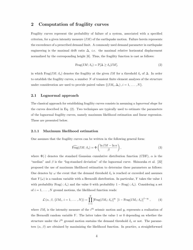
2 Computation of fragility curves
Fragility curves represent the probability of failure of a system, associated with a specified
criterion, for a given intensity measure (IM) of the earthquake motion. Failure herein represents
the exceedence of a prescribed demand limit. A commonly used demand parameter in earthquake
engineering is the maximal drift ratio ∆, i.e. the maximal relative horizontal displacement
normalized by the corresponding height [6]. Thus, the fragility function is cast as follows:
Frag(IM ; δo) = P[∆ ≥ δo|IM ], (2)
in which Frag(IM ; δo) denotes the fragility at the given IM for a threshold δo of ∆. In order
to establish the fragility curves, a number N of transient finite element analyses of the structure
under consideration are used to provide paired values {(IMi,∆i) , i = 1, . . . , N}.
2.1 Lognormal approach
The classical approach for establishing fragility curves consists in assuming a lognormal shape for
the curves described in Eq. (2). Two techniques are typically used to estimate the parameters
of the lognormal fragility curves, namely maximum likelihood estimation and linear regression.
These are presented below.
2.1.1 Maximum likelihood estimation
One assumes that the fragility curves can be written in the following general form:
Frag(IM ; δo) = Φ
(ln IM − lnα
β
), (3)
where Φ(·) denotes the standard Gaussian cumulative distribution function (CDF), α is the
“median” and β is the “log-standard deviation” of the lognormal curve. Shinozuka et al. [22]
proposed the use of maximum likelihood estimation to determine these parameters as follows:
One denotes by ω the event that the demand threshold δo is reached or exceeded and assumes
that Y (ω) is a random variable with a Bernoulli distribution. In particular, Y takes the value 1
with probability Frag(·; δo) and the value 0 with probability 1 − Frag(·; δo). Considering a set
of i = 1, . . . , N ground motions, the likelihood function reads:
L (α, β, {IMi, i = 1, . . . , N}) =
N∏i=1
[Frag(IMi; δo)]yi [1− Frag(IMi; δo)]
1−yi , (4)
where IMi is the intensity measure of the ith seismic motion and yi represents a realization of
the Bernoulli random variable Y . The latter takes the value 1 or 0 depending on whether the
structure under the ith ground motion sustains the demand threshold δo or not. The parame-
ters (α, β) are obtained by maximizing the likelihood function. In practice, a straightforward
4

optimization algorithm is applied on the log-likelihood function:
{α∗; β∗}T = arg max lnL (α, β, {IMi, i = 1, . . . , N}) . (5)
2.1.2 Linear regression
One first assumes a probabilistic seismic demand model, which relates a structural response quan-
tity of interest (herein drift ratio) to an intensity measure of the earthquake motion. Specifically,
the demand ∆ is assumed to follow a lognormal distribution of which the log-mean value is a
linear function of ln IM , leading to:
ln ∆ = A ln IM +B + ζ Z, (6)
where Z ∼ N (0, 1) is a standard normal variable. Parameters A and B are determined by means
of ordinary least squares estimation in a log-log scale. Parameter ζ is obtained by:
ζ2 =
N∑i=1
e2i / (N − 2) , (7)
where ei the residual between the actual value ln ∆ and the value predicted by the linear model:
ei = ln ∆i −A ln (IMi)−B. Then, Eq. (2) rewrites:
Frag(IM ; δo) = P [ln ∆ ≥ ln δo] = 1− P [ln ∆ ≤ ln δo]
= Φ
(ln IM − (ln δo −B) /A
ζ/A
).
(8)
A comparison to Eq. (3) shows that the median and log-standard deviation of the lognormal
fragility curve in Eq. (8) are α = exp [(ln δo −B) /A] and β = ζ/A, respectively. This approach
to fragility estimation is widely employed in the literature, see e.g. [23, 31, 32, 33] among others.
The two methods described in this section are parametric because they impose the shape of
the fragility curves (Eq. (3) and Eq. (8)), which is that of a lognormal CDF when considered
as a function of IM . We note that by using the linear-regression approach, one accepts two
additional assumptions, namely the linear function for the log-mean value of ∆ and the constant
dispersion (or homoscedasticity) of the residuals independently of the IM level. Effects of these
assumptions have been investigated by Karamlou and Bocchini [28]. In the sequel, we propose
two non-parametric approaches to compute fragility curves without relying on the lognormality
assumption.
2.2 Binned Monte Carlo simulation
Having at hand a large sample set {(IMj ,∆j) , j = 1, . . . , N}, it is possible to use binned Monte
Carlo simulation (bMCS) to compute the fragility curves, as described next. Let us consider a
given abscissa IMo. Within a small bin surrounding IMo, say [IMo − h, IMo + h] one assumes
5
that the maximal drift ∆ is linearly related to the IM . This assumption is exact in the case
of linear structures, but would only be an approximation in the nonlinear case. Therefore, the
maximal drift ∆j , which is related to IMj ∈ [IMo − h, IMo + h], is converted into the drift
∆j(IMo), which is related to the jth input signal scaled to have an intensity measure equal to
IMo:
∆j(IMo) = ∆jIMo
IMj. (9)
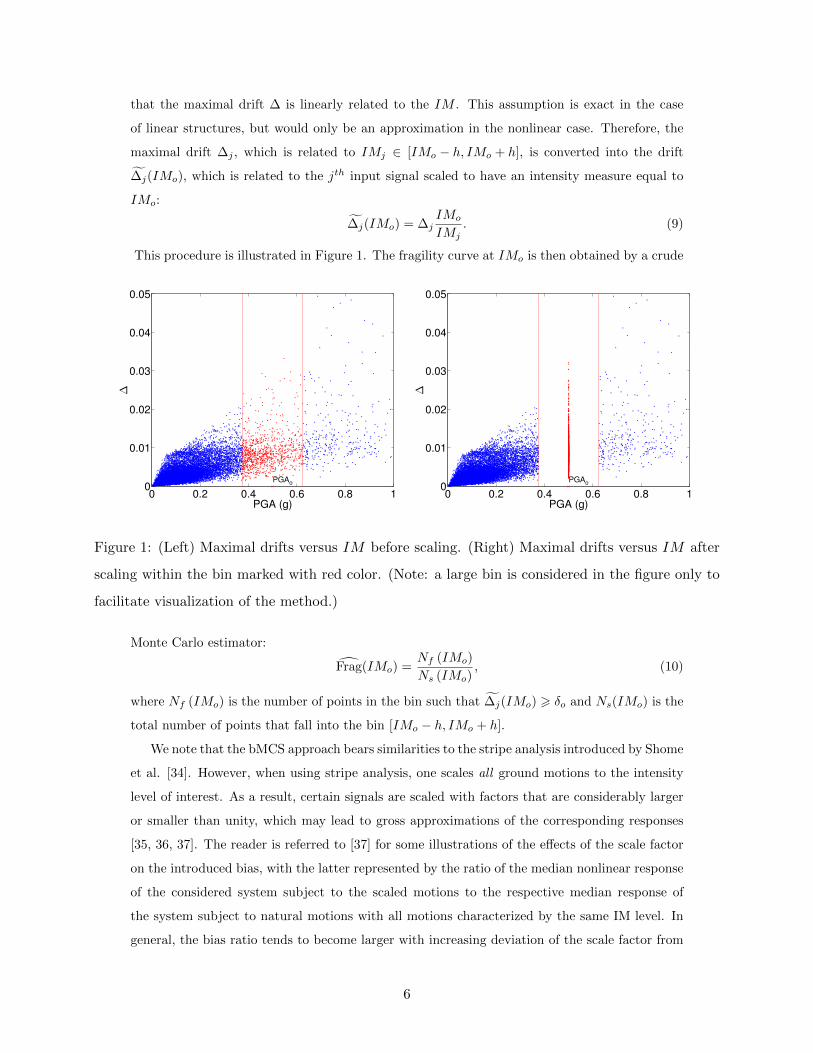
This procedure is illustrated in Figure 1. The fragility curve at IMo is then obtained by a crude
0 0.2 0.4 0.6 0.8 10
0.01
0.02
0.03
0.04
0.05
PGA (g)
∆
PGAo
0 0.2 0.4 0.6 0.8 10
0.01
0.02
0.03
0.04
0.05
PGA (g)
∆
PGAo
Figure 1: (Left) Maximal drifts versus IM before scaling. (Right) Maximal drifts versus IM after
scaling within the bin marked with red color. (Note: a large bin is considered in the figure only to
facilitate visualization of the method.)
Monte Carlo estimator:
Frag(IMo) =Nf (IMo)
Ns (IMo), (10)
where Nf (IMo) is the number of points in the bin such that ∆j(IMo) > δo and Ns(IMo) is the
total number of points that fall into the bin [IMo − h, IMo + h].
We note that the bMCS approach bears similarities to the stripe analysis introduced by Shome
et al. [34]. However, when using stripe analysis, one scales all ground motions to the intensity
level of interest. As a result, certain signals are scaled with factors that are considerably larger
or smaller than unity, which may lead to gross approximations of the corresponding responses
[35, 36, 37]. The reader is referred to [37] for some illustrations of the effects of the scale factor
on the introduced bias, with the latter represented by the ratio of the median nonlinear response
of the considered system subject to the scaled motions to the respective median response of
the system subject to natural motions with all motions characterized by the same IM level. In
general, the bias ratio tends to become larger with increasing deviation of the scale factor from
6

unity. On the other hand, the scaling in binned MCS is confined in the vicinity of the intensity
level IMo, where the vicinity is defined by the bin width 2h chosen so that the scale factors are
close to unity. Accordingly, the bias due to ground motion scaling is negligible in bMCS.
Following the above discussion, it should be noted that bias from scaling can be avoided by
a proper selection of ground motions. For instance, Shome et al. [34] showed that the scaling
of motions that correspond to a narrow interval of earthquake magnitudes and source-to-site
distances does not introduce bias into the nonlinear response estimates. Furthermore, Luco and
Bazzurro [35] showed that the bias can be reduced by selecting records that have appropriate
response spectrum shapes. According to Bazzurro et al. [38] and Vamvatsikos and Cornell [39],
the existence of scale-induced bias also depends on several other factors, such as the structural
characteristics and the considered intensity and damage measures. The topic of ground motion
scaling is complex and falls outside the scope of this paper. We underline that by using the
bMCS approach, we avoid introducing bias in the results independently of the ground motion
characteristics or other factors. In the following case studies, the resulting fragility curves serve as
reference for assessing the accuracy of the various considered techniques for fragility estimation.
2.3 Kernel density estimation
The fragility function defined in Eq. (2) may be reformulated using the conditional probability
density function (PDF) f∆|IM as follows:
Frag(a; δo) = P (∆ ≥ δo|IM = a) =
+∞∫δo
f∆(δ|IM = a) dδ. (11)
By definition, this conditional PDF is given as:
f∆(δ|IM = a) =f∆,IM (δ, a)
fIM (a), (12)
where f∆,IM (·) is the joint distribution of the vector (∆, IM) and fIM (·) is the marginal dis-
tribution of the IM . If these quantities were known, the fragility function in Eq. (11) would
be obtained by a mere integration. In this section, we propose to determine the joint and
marginal PDFs from a sample set {(IMi,∆i) , i = 1, . . . , N} by means of kernel density esti-
mation (KDE).
For a single random variable X for which a sample set {x1, . . . , xN} is available, the kernel
density estimate of the PDF reads [40]:
fX (x) =1
Nh
N∑i=1
K
(x− xih
), (13)
where h is the bandwidth parameter and K(·) is the kernel function which integrates to one.
Classical kernel functions are the Epanechnikov, uniform, normal and triangular functions. The
7
choice of the kernel is known not to affect strongly the quality of the estimate provided the
sample set is large enough [40]. In case a standard normal PDF is adopted for the kernel, the
kernel density estimate rewrites:
fX (x) =1
Nh
N∑i=1
1
(2π)1/2
exp
[−1
2
(x− xih
)2]. (14)
In contrast, the choice of the bandwidth h is crucial since an inappropriate value of h can lead
to an oversmoothed or undersmoothed PDF estimate [41].
Kernel density estimation may be extended to a random vector X ∈ Rd given an i.i.d sample
{x1, . . . ,xN} [40]:
fX (x) =1
N |H|1/2N∑i=1
K(H−1/2(x− xi)
), (15)
where H is a symmetric positive definite bandwidth matrix with determinant denoted by |H|.
When a multivariate standard normal kernel is adopted, the joint distribution estimate becomes:
fX (x) =1
N |H|1/2N∑i=1
1
(2π)d/2
exp
[−1
2(x− xi)TH−1(x− xi)
], (16)
where (·)T denotes the transposition. For multivariate problems (i.e. X ∈ Rd), the bandwidth
matrix typically belongs to one of the following classes: spherical, ellipsoidal and full matrix,
which respectively contain 1, d and d(d + 1)/2 independent unknown parameters. The matrix
H can be computed by means of plug-in or cross-validation estimators. Both estimators aim at
minimizing the asymptotic mean integrated squared error (MISE):
MISE = E
∫Rd
[fX(x; H)− fX(x)
]2dx
. (17)
However, the two approaches differ in the formulation of the numerical approximation of MISE.
For further details, the reader is referred to Duong [41]. In the most general case when the
correlations between the random variables are not known, the full matrix should be used. In
this case, the smoothed cross-validation estimator is the most reliable among the cross-validation
methods [42].
Eq. (14) is used to estimate the marginal PDF of the IM , namely fIM (a), from a sample
{IMi, i = 1, . . . , N}:
fIM (a) =1
(2π)1/2
NhIM
N∑i=1
exp
[−1
2
(a− IM i
hIM
)2]. (18)
Eq. (16) is used to estimate the joint PDF f∆,IM (δ, a) from the data pairs {(IMi, ∆i), i = 1, . . . , N}:
f∆,IM (δ, a) =1
2πN |H|1/2N∑i=1
exp
−1
2
δ −∆i
a− IMi
T
H−1
δ −∆i
a− IMi
. (19)
8

The conditional PDF f∆(δ|IM = a) is eventually estimated by plugging the estimations of
the numerator and denominator in Eq. (12). The proposed estimator of the fragility function
eventually reads:
Frag(a; δo) =hIM
(2π |H|)1/2
+∞∫δo
N∑i=1
exp
−1
2
δ −∆i
a− IMi
T
H−1
δ −∆i
a− IMi
dδ
N∑i=1
exp
[−1
2
(a− IM i
hIM
)2] . (20)
The choice of the bandwidth parameter h and the bandwidth matrix H plays a crucial role
in the estimation of fragility curves, as seen in Eq. (20). In the above formulation, the same
bandwidth is considered for the whole range of the IM values. However, there are typically few
observations available corresponding to the upper tail of the distribution of the IM . This is due
to the fact that the annual frequency of seismic motions with IM values in the respective range
(e.g. PGA exceeding 1g) is low (see e.g. [43]). This is also the case when synthetic ground
motions are used, since these are generated consistently with statistical features of recorded
motions. Preliminary investigations have shown that by applying the KDE method on the data
in the original scale, the fragility curves for the higher demand thresholds tend to be unstable
in their upper tails [44]. To reduce effects from the scarcity of observations at large IM values,
we propose the use of KDE in the logarithmic scale, as described next.
Let us consider two random variables X, Y with positive supports, and their logarithmic
transformations U = lnX and V = lnY . One has:
+∞∫y0
fY (y|X = x) dy =
+∞∫y0
fX,Y (x, y)
fX(x)dy =
+∞∫ln y0
fU,V (u, v)
x yfU (u)
x
y dv =
+∞∫ln y0
fV (v|U = u) dv. (21)
Accordingly, by substituting X = IM and Y = ∆, the fragility function in Eq. (11) can be
obtained in terms of U = ln IM and V = ln ∆ as:
Frag(a; δo) =
+∞∫δo
f∆(δ|IM = a) dδ =
+∞∫ln δo
fV (v|U = ln a) dv. (22)
The use of a constant bandwidth in the logarithmic scale is equivalent to the use of a varying
bandwidth in the original scale, with larger bandwidths corresponding to larger values of IM .
The resulting fragility curves are smoother than those obtained by applying KDE with the data
in the original scale.
2.4 Epistemic uncertainty of fragility curves
It is of major importance in fragility analysis to investigate the variability in the estimated curves
arising due to epistemic uncertainty. This is because a fragility curve is always computed based
9

on a limited amount of data, i.e. a limited number of ground motions and related structural
analyses. Large epistemic uncertainties may affect significantly the total variability of the seismic
risk assessment outcomes. Characterizing and propagating epistemic uncertainties in seismic loss
estimation has therefore attracted attention from several researchers [2, 45, 46].
The theoretical approach to determine the variability of an estimator relies on repeating the
estimation with an ensemble of different random samples. However, this approach is not feasible
in earthquake engineering because of the high computational cost. In this context, the bootstrap
resampling technique is deemed appropriate [2]. Given a set of observations X = (X1, . . . ,Xn)
of X following an unknown probability distribution, the bootstrap method allows estimation of
the statistics of a random variable that depends on X in terms of the observed data X and their
empirical distribution [47].
To estimate statistics of the fragility curves with the bootstrap method, we first draw M inde-
pendent random samples with replacement from the original data set {(IMi,∆i) , i = 1, . . . , N}.
These represent the so-called bootstrap samples. Each bootstrap sample has the same size N
as the original sample, but the observations are different: in a particular sample, some of the
original observations may appear multiple times while others may be missing. Next, we compute
the fragility curves for each bootstrap sample using the approaches in Sections 2.1, 2.2 and 2.3.
Finally, we perform statistical analysis of the so-obtained M bootstrap curves. In the subse-
quent example illustration, the above procedure is employed to evaluate the median and 95%
confidence intervals of the estimated fragility curves and also, to assess the variability of the IM
value corresponding to a 50% probability of failure.
3 Synthetic ground motions
3.1 Properties of recorded ground motions
Let us consider a recorded earthquake accelerogram a(t), t ∈ [0, T ] where T is the total duration
of the motion. The peak ground acceleration is PGA = maxt∈[0,T ]
|a(t)|. The Arias intensity Ia is
defined as:
Ia =π
2g
T∫0
a2(t) dt. (23)
Defining the cumulative square acceleration as:
I(t) =π
2g
t∫0
a2(τ) dτ , (24)
one determines the time instant tα by:
tα : I(tα) = αIa α ∈ [0, 1]. (25)
10
In addition to the Arias intensity, important properties of the accelerogram in the time domain
include the effective duration, defined as D5−95 = t95%− t5%, and the instant tmid at the middle
of the strong-shaking phase [49]. Based on the investigation of a set of recorded ground motions,
Rezaeian and Der Kiureghian [49] proposed that tmid is taken as the time when 45% of the Arias
intensity is reached i.e. tmid ≡ t45%.
Other important properties of the accelerogram are related to its frequency content. Analyses
of recorded ground motions indicate that the time evolution of the predominant frequency of an
accelerogram can be represented by a linear model, whereas its bandwidth can be considered
constant [30]. Rezaeian and Der Kiureghian [30] describe the evolution of the predominant
frequency in terms of its value ωmid at the time instant tmid and the slope of the evolution ω′.
The same authors describe the bandwidth in terns of the bandwidth parameter ζ. A procedure
for estimating the parameters ωmid, ω′ and ζ for a given accelerogram is presented in [30],
whereas a simplified version is proposed in [49].
Next, we describe a method for simulating synthetic accelerograms in terms of the set of pa-
rameters (Ia, D5−95, tmid, ωmid, ω′, ζf ); this method will be used to generate the seismic motions
in a subsequent case study.
3.2 Simulation of synthetic ground motions
The use of synthetic ground motions has been attracting an increasing interest from the earth-
quake engineering community. This practice overcomes the limitations posed by the small num-
ber of records typically available for a design scenario and avoids the need to scale the motions.
Use of synthetic ground motions allows one to investigate the structural response for a large
number of motions, which is nowadays feasible with the available computer resources (see e.g.
[48]).
Different stochastic ground motion models can be found in the literature, which can be
classified in three types [49]: record-based parameterized models that are fit to recorded motions,
source-based models that consider the physics of the source mechanism and wave travel-path, and
hybrid models that combine elements from both source- and record-based models. Vetter and
Taflanidis [50] compared the source-based model by Boore [51] with the record-based model by
Rezaeian and Der Kiureghian [49] with respect to the estimated seismic risks. It was found that
the latter leads to higher estimated risks for low-magnitude events, but the risks are quantified
in a consistent manner exhibiting correlation with the hazard characteristics. This model is
employed in the present study to generate a large suite of synthetic ground motions that are used
to obtain pairs of the ground motion intensity measure and the associated structural response,
(IM,∆), in order to conduct fragility analysis. The approach, originally proposed in [30], is
summarized below.
11

The seismic acceleration a(t) is represented as a non-stationary process. In particular, the
non-stationarity is separated into two components, namely a spectral and a temporal one, by
means of a modulated filtered Gaussian white noise:
a(t) =q(t,α)
σh(t)
t∫0
h [t− τ,λ (τ)]ω(τ) dτ, (26)
in which q(t,α) is the deterministic non-negative modulating function, the integral is the non-
stationary response of a linear filter subject to a Gaussian white-noise excitation and σh(t) is the
standard deviation of the response process. The Gaussian white-noise process denoted by ω(τ)
will pass through a filter h [t− τ,λ(τ)], which is selected as the pseudo-acceleration response of
a single-degree-of-freedom (SDOF) linear oscillator:
h [t− τ,λ(τ)] = 0 for t < τ
h [t− τ,λ(τ)] =ωf (τ)√1− ζ2
f (τ)exp [−ζf (τ)ωf (τ)(t− τ)] sin
[ωf (τ)
√1− ζ2
f (τ)(t− τ)]
for t ≥ τ.
(27)
In the above equation, λ(τ) = (ωf (τ), ζf (τ)) is the vector of time-varying parameters of the filter
h, with ωf (τ) and ζf (τ) respectively denoting the filter’s natural frequency and damping ratio
at instant τ . Note that ωf (τ) corresponds to the evolving predominant frequency of the ground
motion represented, while ζf (τ) corresponds to the bandwidth parameter of the motion. As
noted in Section 3.1, ζf (τ) may be taken as a constant (ζf (τ) ≡ ζ), while ωf (τ) is approximated
as a linear function:
ωf (τ) = ωmid + ω′(τ − tmid), (28)
where tmid, ωmid and ω′ are as defined in Section 3.1. After being normalized by the standard
deviation σh(t), the integral in Eq. (26) becomes a unit-variance process with time-varying
frequency and constant bandwidth. The non-stationarity in intensity is then captured by the
modulating function q(t,α), which determines the shape, intensity and duration T of the signal.
This is typically described by a Gamma-like function [49]:
q(t,α) = α1tα2−1exp(−α3t), (29)
where α = {α1, α2, α3} is directly related to the energy content of the signal through the
quantities Ia, D5−95 and tmid defined in Section 3.1 (see [49] for details).
For computational purposes, the acceleration in Eq. (26) can be discretized as follows:
a(t) = q(t,α)
n∑i=1
si (t,λ(ti)) Ui, (30)
where the standard normal random variable Ui represents an impulse at instant ti = i× T
n, i =
12

1, . . . , n, (T is the total duration) and si(t,λ(ti)) is given by:
si(t,λ(ti)) =h [t− ti,λ(ti)]√∑ij=1 h
2 [t− tj ,λ(tj)]. (31)
As a summary, the considered seismic motion generation model consists of the three temporal
parameters (α1, α2, α3), which are related to (Ia, D5−95, tmid), the three spectral parameters
(ωmid, ω′, ζf ) and the standard Gaussian random vector U of size n. Rezaeian and Der Ki-
ureghian [49] proposed a methodology for determining the temporal and spectral parameters
according to earthquake and site characteristics, i.e. the type of faulting of the earthquake
(strike-slip fault or reverse fault), the closest distance from the recording site to the ruptured
area and the shear-wave velocity of the top 30 m of the site soil. For the sake of simplicity,
in this paper these parameters are directly generated from the statistical models given in [49],
which are obtained from analysis of a large set of recorded ground motions.
4 Steel frame structure subject to synthetic ground mo-
tions
4.1 Problem setup
We determine the fragility curves for the three-storey three-span steel frame shown in Figure 2.
The dimensions of the structure are: storey-height H = 3 m, span-length L = 5 m. The vertical
load consists of dead load (weight of frame elements and supported floors) and live load (in ac-
cordance with Eurocode 1 [52]) resulting in a total distributed load on the beams q = 20 kN/m.
In the preliminary design stage, the standard European I beams with designation IPE 300 A and
IPE 330 O are chosen respectively for the beams and columns. The steel material has a non-
linear isotropic hardening behavior following the uniaxial Giuffre-Menegotto-Pinto steel model
as implemented in the finite element software OpenSees [53]. Ellingwood and Kinali [5] have
shown that uncertainty in the properties of the steel material has a negligible effect on seismic
fragility curves. Therefore, the mean material properties are used in the subsequent fragility
analysis: E0 = 210, 000 MPa for the Young’s modulus (initial elastic tangent in the stress-strain
curve), fy = 264 MPa for the yield strength [54, 55] and b = 0.01 for the strain hardening
ratio (ratio of post-yield to initial tangent in the stress-strain curve). Figure 2 depicts the hys-
teretic behavior of the steel material at a specified section for an example ground motion. The
structural components are modelled with nonlinear force-based beam-column elements charac-
terized by distributed plasticity along their lengths, while use of fiber sections allows modelling
the plasticity over the element cross-sections [56]. The connections between structural elements
are modeled with rigid nodes. The first two natural periods of the building obtained by modal
13
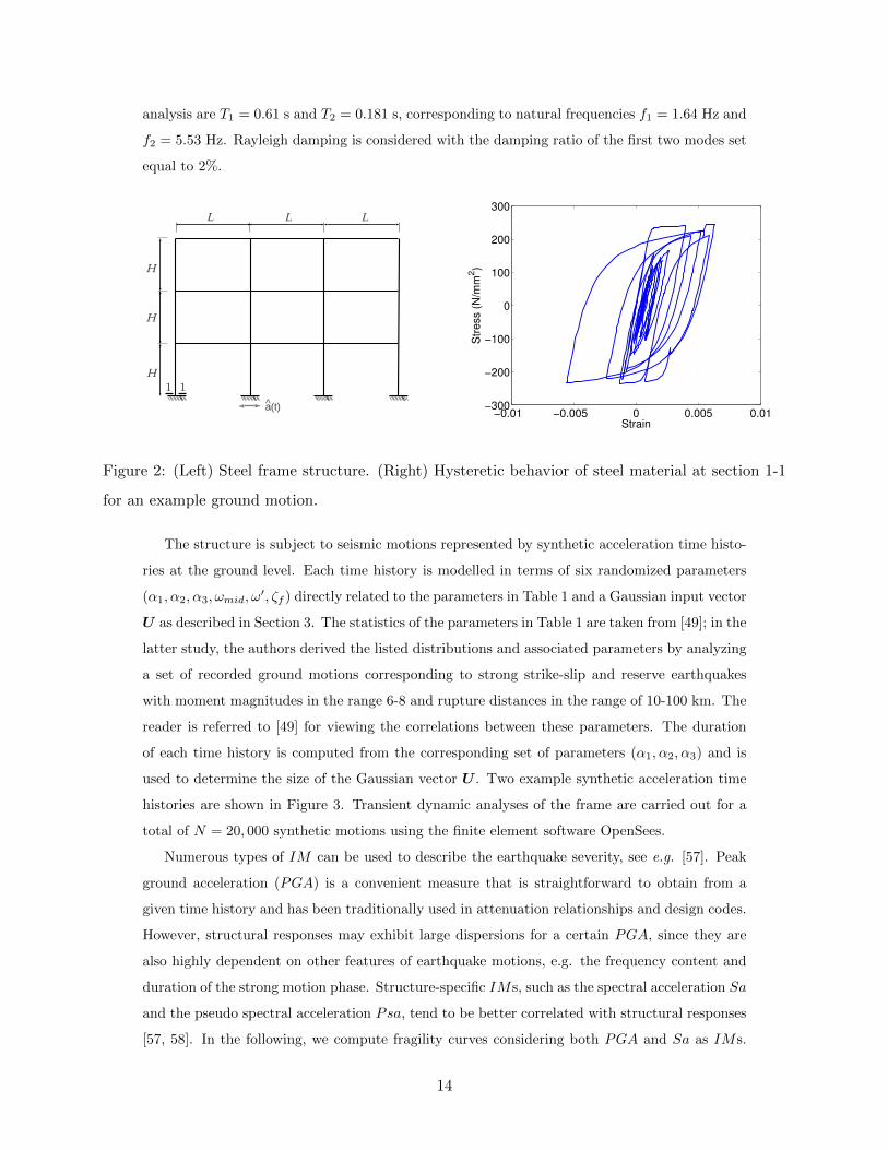
analysis are T1 = 0.61 s and T2 = 0.181 s, corresponding to natural frequencies f1 = 1.64 Hz and
f2 = 5.53 Hz. Rayleigh damping is considered with the damping ratio of the first two modes set
equal to 2%.
LHHH
a(t)^
L L
1 1−0.01 −0.005 0 0.005 0.01
−300
−200
−100
0
100
200
300
Strain
Str
ess (
N/m
m2)
Figure 2: (Left) Steel frame structure. (Right) Hysteretic behavior of steel material at section 1-1
for an example ground motion.
The structure is subject to seismic motions represented by synthetic acceleration time histo-
ries at the ground level. Each time history is modelled in terms of six randomized parameters
(α1, α2, α3, ωmid, ω′, ζf ) directly related to the parameters in Table 1 and a Gaussian input vector
U as described in Section 3. The statistics of the parameters in Table 1 are taken from [49]; in the
latter study, the authors derived the listed distributions and associated parameters by analyzing
a set of recorded ground motions corresponding to strong strike-slip and reserve earthquakes
with moment magnitudes in the range 6-8 and rupture distances in the range of 10-100 km. The
reader is referred to [49] for viewing the correlations between these parameters. The duration
of each time history is computed from the corresponding set of parameters (α1, α2, α3) and is
used to determine the size of the Gaussian vector U . Two example synthetic acceleration time
histories are shown in Figure 3. Transient dynamic analyses of the frame are carried out for a
total of N = 20, 000 synthetic motions using the finite element software OpenSees.
Numerous types of IM can be used to describe the earthquake severity, see e.g. [57]. Peak
ground acceleration (PGA) is a convenient measure that is straightforward to obtain from a
given time history and has been traditionally used in attenuation relationships and design codes.
However, structural responses may exhibit large dispersions for a certain PGA, since they are
also highly dependent on other features of earthquake motions, e.g. the frequency content and
duration of the strong motion phase. Structure-specific IMs, such as the spectral acceleration Sa
and the pseudo spectral acceleration Psa, tend to be better correlated with structural responses
[57, 58]. In the following, we compute fragility curves considering both PGA and Sa as IMs.
14

Table 1: Statistics of synthetic ground motion parameters according to [49].
Parameter Distribution Support µX σX
Ia (s×g) Lognormal (0, +∞) 0.0468 0.164
D5−95 (s) Beta [5, 45] 17.3 9.31
tmid (s) Beta [0.5, 40] 12.4 7.44
ωmid/2π (Hz) Gamma (0, +∞) 5.87 3.11
ω′/2π (Hz) Two-sided exponential [-2, 0.5] -0.089 0.185
ζf Beta [0.02, 1] 0.213 0.143
0 5 10 15 20−1
−0.5
0
0.5
1
t (s)
Acce
lera
tio
n (
g)
0 5 10 15 20 25 30−1
−0.5
0
0.5
1
t (s)
Acce
lera
tio
n (
g)
Figure 3: Examples of synthetic ground motions.
Sa represents Sa(T1) i.e. the spectral acceleration for a single-degree-of-freedom system with
period equal to the fundamental period T1 of the frame and viscous damping ratio equal to 2%.
The engineering demand parameter commonly considered in fragility analysis of steel build-
ings is the maximal inter-storey drift ratio, i.e. the maximal difference of horizontal displace-
ments between consecutive storeys normalized by the storey height (see e.g. [5, 59, 60]). Accord-
ingly, we herein develop fragility curves for three different thresholds of the maximal inter-storey
drift ratio over the frame. To gain insight into structural performance, we consider the thresholds
0.7%, 1.5% and 2.5%, which are associated with different damage states in seismic codes. In
particular, the thresholds 0.7% and 2.5% are recommended in [61] to respectively characterize
light and moderate damage for steel frames, while the threshold 1.5% corresponds to the damage
limitation requirement for buildings with ductile non-structural elements according to Eurocode
8 [62]. These descriptions only serve as rough damage indicators, since the relationship between
15
drift limit and damage in the PBEE framework is probabilistic.
4.2 Fragility curves
As described in Section 2, the lognormal approach relies on assuming that the fragility curves have
the shape of a lognormal CDF and estimating the parameters of this CDF. Using the maximum
likelihood estimation (MLE) approach, the observed failures for each drift threshold are modeled
as outcomes of a Bernoulli experiment and the parameters (α, β) of the fragility curves are
determined by maximizing the respective likelihood function. Using the linear regression (LR)
technique, the parameters of the lognormal curves are derived by fitting a linear model to the
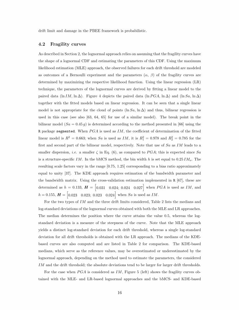
paired data (ln IM, ln ∆). Figure 4 depicts the paired data (lnPGA, ln ∆) and (lnSa, ln ∆)
together with the fitted models based on linear regression. It can be seen that a single linear
model is not appropriate for the cloud of points (lnSa, ln ∆) and thus, bilinear regression is
used in this case (see also [63, 64, 65] for use of a similar model). The break point in the
bilinear model (Sa = 0.45 g) is determined according to the method presented in [66] using the
R package segmented. When PGA is used as IM , the coefficient of determination of the fitted
linear model is R2 = 0.663; when Sa is used as IM , it is R21 = 0.978 and R2
2 = 0.785 for the
first and second part of the bilinear model, respectively. Note that use of Sa as IM leads to a
smaller dispersion, i.e. a smaller ζ in Eq. (6), as compared to PGA; this is expected since Sa
is a structure-specific IM . In the bMCS method, the bin width h is set equal to 0.25 IMo. The
resulting scale factors vary in the range [0.75, 1.25] corresponding to a bias ratio approximately
equal to unity [37]. The KDE approach requires estimation of the bandwidth parameter and
the bandwidth matrix. Using the cross-validation estimation implemented in R [67], these are
determined as h = 0.133, H =[0.031 0.024; 0.024 0.027
]when PGA is used as IM , and
h = 0.155, H =[0.023 0.023; 0.023 0.024
]when Sa is used as IM .
For the two types of IM and the three drift limits considered, Table 2 lists the medians and
log-standard deviations of the lognormal curves obtained with both the MLE and LR approaches.
The median determines the position where the curve attains the value 0.5, whereas the log-
standard deviation is a measure of the steepness of the curve. Note that the MLE approach
yields a distinct log-standard deviation for each drift threshold, whereas a single log-standard
deviation for all drift thresholds is obtained with the LR approach. The medians of the KDE-
based curves are also computed and are listed in Table 2 for comparison. The KDE-based
medians, which serve as the reference values, may be overestimated or underestimated by the
lognormal approach, depending on the method used to estimate the parameters, the considered
IM and the drift threshold; the absolute deviations tend to be larger for larger drift thresholds.
For the case when PGA is considered as IM , Figure 5 (left) shows the fragility curves ob-
tained with the MLE- and LR-based lognormal approaches and the bMCS- and KDE-based
16
Table 2: Steel frame structure - Parameters of the obtained fragility curves.
PGA Sa
δo Approach Median Log-std Median Log-std
0.7%
MLE 0.35 g 0.70 0.49 g 0.36
LR 0.37 g 0.64 0.44 g 0.13
KDE 0.36 g 0.45 g
1.5%
MLE 1.10 g 0.56 1.66 g 0.31
LR 0.87 g 0.64 1.47 g 0.24
KDE 1.08 g 1.53 g
2.5%
MLE 1.76 g 0.56 2.82 g 0.37
LR 1.55 g 0.64 3.29 g 0.24
KDE 1.82 g 3.04 g
10−3
10−2
10−1
100
101
10−5
10−4
10−3
10−2
10−1
PGA (g)
∆
Cloud of points
ln ∆=0.8889 ln PGA−4.08
10−3
10−2
10−1
100
101
10−5
10−4
10−3
10−2
10−1
Sa (g)
∆
Cloud of points
ln ∆=0.96782 ln Sa−4.1772
ln ∆=0.63486 ln Sa−4.4457
Figure 4: Paired data {(IMi,∆i) , i = 1, . . . , N} and fitted models in log-scale (the units of the
variables in the fitted models are the same as in the axes of the graphs).
non-parametric approaches. One first observes a remarkable consistency between the curves
obtained with the two non-parametric approaches despite the distinct differences in the under-
lying algorithms. This validates the accuracy of the proposed methods. For the lower threshold
(δo = 0.7%), both parametric curves are in good agreement with the non-parametric ones. For
the two higher thresholds, the LR-based lognormal curves exhibit significant deviations from
the non-parametric ones leading to an overestimation of the failure probabilities. Note that for
δo = 1.5% and δo = 2.5%, the median PGA (leading to 50% probability of exceedance) is respec-
17
tively underestimated by 19% and 15% when the LR aproach is used (see Table 2). In contrast,
the MLE-based lognormal curves are in a fair agreement with their non-parametric counterparts
with the largest discrepancies observed for the highest threshold δo = 2.5%.
Figure 5 (right) shows the resulting fragility curves when Sa is considered as IM . The
non-parametric curves based on bMCS and KDE remain consistent independently of the drift
threshold. For δo = 0.7%, the fragility curves are steep, which is due to the strong correlation
between Sa and ∆ when the structure behaves linearly. For this threshold, the LR-based curve is
closer to the non-parametric curves than the MLE-based one. For the two larger thresholds, the
MLE-based curves are fairly accurate, whereas the LR-based curves exhibit significant deviations
from their non-parametric counterparts. In particular, the LR-based curves overestimate the
failure probabilities for δo = 1.5% and underestimate the failure probabilities for δo = 2.5%.
Note that for δo = 1.5%, the median Sa is underestimated by 4%, whereas for δo = 1.5%, the
median Sa is overestimated by 8% when the LR aproach is used (see Table 2).
0 0.5 1 1.5 20
0.2
0.4
0.6
0.8
1δo =0.007
δo =0.015
δo =0.025
PGA (g)
Pro
ba
bili
ty o
f fa
ilure
LRMLEbMCSKDE
0 1 2 3 40
0.2
0.4
0.6
0.8
1δo =0.007
δo =0.015
δo =0.025
Sa (g)
Pro
ba
bili
ty o
f fa
ilure
LRMLEbMCSKDE
Figure 5: Fragility curves with parametric and non-parametric approaches using PGA and Sa as
intensity measures (LR: linear regression; MLE: maximum likelihood estimation; bMCS: binned
Monte Carlo simulation; KDE: kernel density estimation).
Summarizing the above results, the MLE-based lognormal approach yields fragility curves
that are overall close to the non-parametric ones; however, it smooths out some details of the
curves that can be obtained with the non-parametric approaches. On the contrary, the LR-based
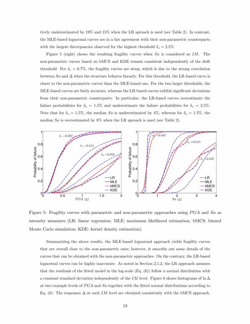
lognormal curves can be highly inaccurate. As noted in Section 2.1.2, the LR approach assumes
that the residuals of the fitted model in the log-scale (Eq. (6)) follow a normal distribution with
a constant standard deviation independently of the IM level. Figure 6 shows histograms of ln ∆
at two example levels of PGA and Sa together with the fitted normal distributions according to
Eq. (6). The responses ∆ at each IM level are obtained consistently with the bMCS approach.
18

Obviously, the assumption of a normal distribution is not valid, which is more pronounced when
Sa is used as IM . This explains the inaccuracy of the LR-based fragility curves for both types
of IM , despite the relatively high coefficients of determination of the fitted models in the case
of Sa.
−7 −6 −5 −4 −30
0.2
0.4
0.6
0.8
1
1.2
1.4
ln ∆
Pro
ba
bili
ty d
en
sity
Histogram
Normal fit
(A) PGA = 0.5 g
−6 −5 −4 −3 −20
0.2
0.4
0.6
0.8
1
1.2
1.4
ln ∆P
rob
ab
ility
de
nsity
Histogram
Normal fit
(B) PGA = 1.5 g
−5.5 −5 −4.5 −40
5
10
15
20
ln ∆
Pro
babili
ty d
ensity
Histogram
Normal fit
(C) Sa = 0.5 g
−5 −4.5 −4 −3.5 −30
0.5
1
1.5
2
2.5
3
ln ∆
Pro
ba
bili
ty d
en
sity
Histogram
Normal fit
(D) Sa = 1.5 g
Figure 6: Histograms and fitted normal distributions for ln ∆ at two levels of PGA and Sa.
4.3 Estimation of epistemic uncertainty by bootstrap resampling
In the following, we use the bootstrap resampling technique (see Section 2.4) to investigate
the epistemic uncertainty in the fragility curves estimated with the proposed non-parametric
approaches.
We examine the stability of the estimated curves by comparing those with the bootstrap
19
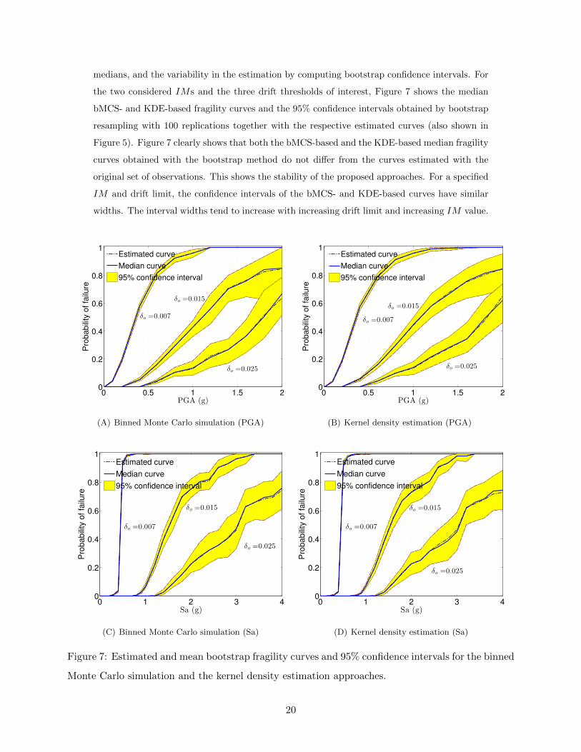
medians, and the variability in the estimation by computing bootstrap confidence intervals. For
the two considered IMs and the three drift thresholds of interest, Figure 7 shows the median
bMCS- and KDE-based fragility curves and the 95% confidence intervals obtained by bootstrap
resampling with 100 replications together with the respective estimated curves (also shown in
Figure 5). Figure 7 clearly shows that both the bMCS-based and the KDE-based median fragility
curves obtained with the bootstrap method do not differ from the curves estimated with the
original set of observations. This shows the stability of the proposed approaches. For a specified
IM and drift limit, the confidence intervals of the bMCS- and KDE-based curves have similar
widths. The interval widths tend to increase with increasing drift limit and increasing IM value.
0 0.5 1 1.5 20
0.2
0.4
0.6
0.8
1
PGA (g)
Pro
ba
bili
ty o
f fa
ilure
δo =0.007
δo =0.015
δo =0.025
Estimated curve
Median curve
95% confidence interval
(A) Binned Monte Carlo simulation (PGA)
0 0.5 1 1.5 20
0.2
0.4
0.6
0.8
1
PGA (g)
Pro
ba
bili
ty o
f fa
ilure
δo =0.007
δo =0.015
δo =0.025
Estimated curve
Median curve
95% confidence interval
(B) Kernel density estimation (PGA)
0 1 2 3 40
0.2
0.4
0.6
0.8
1
Sa (g)
Pro
ba
bili
ty o
f fa
ilure
δo =0.007
δo =0.015
δo =0.025
Estimated curve
Median curve
95% confidence interval
(C) Binned Monte Carlo simulation (Sa)
0 1 2 3 40
0.2
0.4
0.6
0.8
1
Sa (g)
Pro
ba
bili
ty o
f fa
ilure
δo =0.007
δo =0.015
δo =0.025
Estimated curve
Median curve
95% confidence interval
(D) Kernel density estimation (Sa)
Figure 7: Estimated and mean bootstrap fragility curves and 95% confidence intervals for the binned
Monte Carlo simulation and the kernel density estimation approaches.
20

In order to quantify the effects of epistemic uncertainty, one can estimate the variability of
the median IM , i.e. the IM value leading to 50% probability of exceedance. Assuming that the
median IM (PGA or Sa) follows a lognormal distribution [68], the median IM is determined
for each bootstrap curve and the log-standard deviation of the distribution of the median is
computed. Table 3 lists the log-standard deviations of the median IM values for the same cases
as in Figure 7. These results demonstrate that epistemic uncertainty is increasing with increasing
threshold δo. In all cases, the log-standard deviations are relatively small indicating a low level
of epistemic uncertainty, which is due to the large number of transient analyses (N = 20, 000)
considered in this study. Although use of such large sets of ground motions is not typical in
practice, it is useful for the refined analysis presented here.
Table 3: Log-standard deviation of median IM .
δo Approach PGA Sa
0.7%bMCS 0.0003 g 0.005 g
KDE 0.0005 g 0.005 g
1.5%bMCS 0.037 g 0.054 g
KDE 0.037 g 0.050 g
2.5%bMCS 0.114 g 0.090 g
KDE 0.120 g 0.080 g
5 Concrete column subject to recorded ground motions
To demonstrate the comparison between the lognormal and the non-parametric approaches for
the case when fragility curves are based on recorded ground motions, we herein briefly summarize
a case study by the authors originally presented in [29].
In this study, we estimate the fragility of a reinforced concrete column with a uniform cir-
cular cross-section, representing a pier of a typical California highway overpass bridge [63] (see
Figure 8). The column is modelled in the finite element code OpenSees as a fiberized nonlin-
ear beam-column element. For details on the modelling of the concrete material and the steel
reinforcement, the reader is referred to [29]. The loading-unloading behavior and the pushover
curve of the column are shown in Figure 8. Three-dimensional time-history analyses of the
bridge column are conducted for N = 531 earthquake records (each comprising three orthogonal
component accelerograms). These records are obtained from the PEER strong motion database
and cover a wide range of source-to-site distances and earthquake moment magnitudes [63]. The
21

developed fragility curves represent the probability of the maximal drift ratio ∆ in the transverse
direction exceeding specified thresholds δo as a function of the peak ground acceleration PGA or
the pseudo-spectral acceleration Psa corresponding to the first transverse mode (T1 = 0.535 s).
The considered drift ratio thresholds, shown in Table 4, are recommended for the operational
and life safety levels by two different sources [69, 70].
−0.2 −0.1 0 0.1 0.2 0.3 0.4 0.5−1500
−1000
−500
0
500
1000
1500
Displacement (m)
Forc
e (
kN
)
Loading/ unloading behavior
Pushover curve
Figure 8: Bridge configuration [63] and hysteretic behavior.
Table 4: Bridge performance and respective drift-ratio threshold.
Reference Level Description Damage Drift ratio δo
[69] II Operational Minor 0.01
[69] III Life safety Moderate 0.03
[70] II Operational Minor 0.005
[70] III Life safety Moderate 0.015
The fragility curves are established with the MLE-based and LR-based lognormal approaches
and the KDE-based non-parametric approach. Due to the relatively small number of data, the
bMCS method is not considered herein. Figure 9 depicts the clouds of points (IMi, ∆i) in the
logarithmic scale for the two IMs together with the linear fitted models. The coefficients of
determination of the latter are R2 = 0.729 for the case of PGA and R2 = 0.963 for the case of
Psa. Note that for small values of Psa (Psa <0.2 g) a linear function provides a perfect fit,
which is due to the fact that in this range of Psa, the column behavior can be represented by a
22
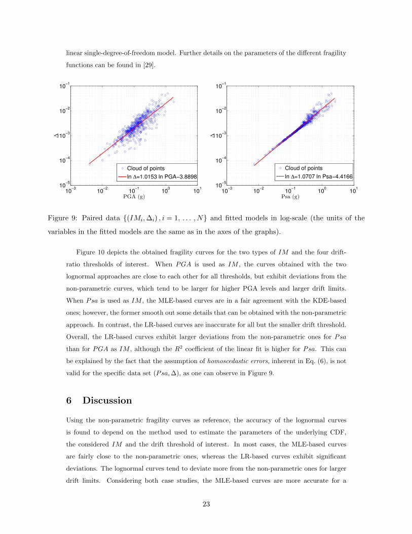
linear single-degree-of-freedom model. Further details on the parameters of the different fragility
functions can be found in [29].
10−3
10−2
10−1
100
101
10−5
10−4
10−3
10−2
10−1
PGA (g)
∆
Cloud of points
ln ∆=1.0153 ln PGA−3.8898
10−3
10−2
10−1
100
101
10−5
10−4
10−3
10−2
10−1
Psa (g)
∆
Cloud of points
ln ∆=1.0707 ln Psa−4.4166
Figure 9: Paired data {(IMi,∆i) , i = 1, . . . , N} and fitted models in log-scale (the units of the
variables in the fitted models are the same as in the axes of the graphs).
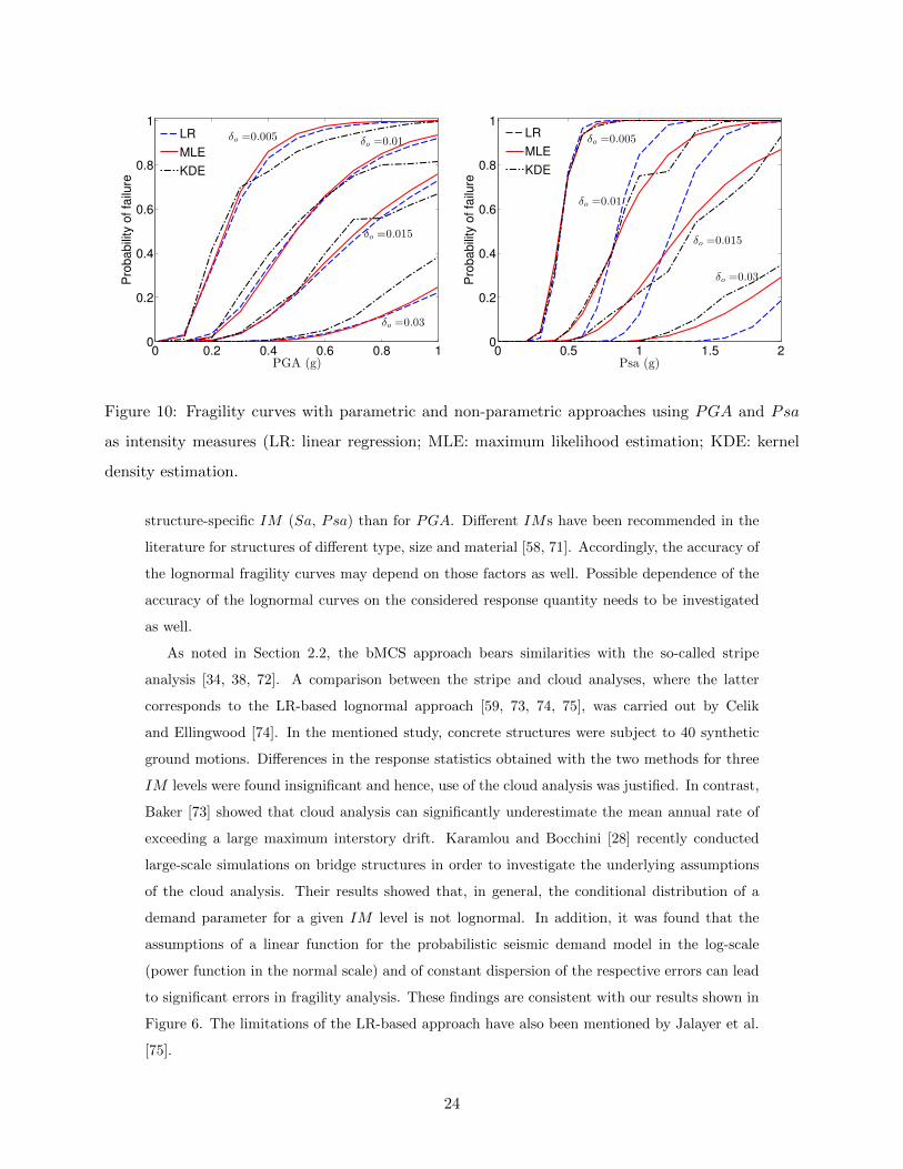
Figure 10 depicts the obtained fragility curves for the two types of IM and the four drift-
ratio thresholds of interest. When PGA is used as IM , the curves obtained with the two
lognormal approaches are close to each other for all thresholds, but exhibit deviations from the
non-parametric curves, which tend to be larger for higher PGA levels and larger drift limits.
When Psa is used as IM , the MLE-based curves are in a fair agreement with the KDE-based
ones; however, the former smooth out some details that can be obtained with the non-parametric
approach. In contrast, the LR-based curves are inaccurate for all but the smaller drift threshold.
Overall, the LR-based curves exhibit larger deviations from the non-parametric ones for Psa
than for PGA as IM , although the R2 coefficient of the linear fit is higher for Psa. This can
be explained by the fact that the assumption of homoscedastic errors, inherent in Eq. (6), is not
valid for the specific data set (Psa,∆), as one can observe in Figure 9.
6 Discussion
Using the non-parametric fragility curves as reference, the accuracy of the lognormal curves
is found to depend on the method used to estimate the parameters of the underlying CDF,
the considered IM and the drift threshold of interest. In most cases, the MLE-based curves
are fairly close to the non-parametric ones, whereas the LR-based curves exhibit significant
deviations. The lognormal curves tend to deviate more from the non-parametric ones for larger
drift limits. Considering both case studies, the MLE-based curves are more accurate for a
23
0 0.2 0.4 0.6 0.8 10
0.2
0.4
0.6
0.8
1δo =0.005
δo =0.01
δo =0.015
δo =0.03
PGA (g)
Pro
ba
bili
ty o
f fa
ilure
LR
MLE
KDE
0 0.5 1 1.5 20
0.2
0.4
0.6
0.8
1
δo =0.005
δo =0.01
δo =0.015
δo =0.03
Psa (g)
Pro
ba
bili
ty o
f fa
ilure
LR
MLE
KDE
Figure 10: Fragility curves with parametric and non-parametric approaches using PGA and Psa
as intensity measures (LR: linear regression; MLE: maximum likelihood estimation; KDE: kernel
density estimation.
structure-specific IM (Sa, Psa) than for PGA. Different IMs have been recommended in the
literature for structures of different type, size and material [58, 71]. Accordingly, the accuracy of
the lognormal fragility curves may depend on those factors as well. Possible dependence of the
accuracy of the lognormal curves on the considered response quantity needs to be investigated
as well.
As noted in Section 2.2, the bMCS approach bears similarities with the so-called stripe
analysis [34, 38, 72]. A comparison between the stripe and cloud analyses, where the latter
corresponds to the LR-based lognormal approach [59, 73, 74, 75], was carried out by Celik
and Ellingwood [74]. In the mentioned study, concrete structures were subject to 40 synthetic
ground motions. Differences in the response statistics obtained with the two methods for three
IM levels were found insignificant and hence, use of the cloud analysis was justified. In contrast,
Baker [73] showed that cloud analysis can significantly underestimate the mean annual rate of
exceeding a large maximum interstory drift. Karamlou and Bocchini [28] recently conducted
large-scale simulations on bridge structures in order to investigate the underlying assumptions
of the cloud analysis. Their results showed that, in general, the conditional distribution of a
demand parameter for a given IM level is not lognormal. In addition, it was found that the
assumptions of a linear function for the probabilistic seismic demand model in the log-scale
(power function in the normal scale) and of constant dispersion of the respective errors can lead
to significant errors in fragility analysis. These findings are consistent with our results shown in
Figure 6. The limitations of the LR-based approach have also been mentioned by Jalayer et al.
[75].
24
Based on the results of our case studies and the above discussion, we recommend the use of
the MLE approach if fragility curves are developed in a parametric manner. The superiority of
the MLE over the LR approach relies on the fact that the former avoids the assumptions of the
linear model and the homoscedasticity of the errors that are inherent in the latter. However,
when a detailed description of the fragility function is important, a non-parametric approach
should be used. The bMCS method requires a large number of data, which can be typically
obtained by use of synthetic motions; note that due to the current computer capacities and the
use of distributed computing, large-scale simulations are becoming increasingly popular among
both researchers and practitioners. On the other hand, the KDE approach can be employed
even with a limited number of recorded motions at hand, as shown in our second case study. We
again emphasize that the two non-parametric approaches lead to almost identical curves in the
case when they could be applied independently with the same (large) dataset.
7 Conclusions
Seismic demand fragility evaluation is one of the basic elements in the framework of performance-
based earthquake engineering (PBEE). At present, the classical lognormal approach is widely
used to establish such fragility curves mainly due to the fact that the lognormality assumption
makes seismic risk analysis more tractable. The approach consists in assigning the shape of a
lognormal cumulative distribution function to the fragility curves. However, the validity of this
assumption remains an open question.
In this paper, we introduce two non-parametric approaches in order to examine the validity
of the classical lognormal approach, namely the binned Monte Carlo simulation and the kernel
density estimation. The former computes the crude Monte Carlo estimators for small subsets
of ground motions with similar values of a selected intensity measure, while the latter estimates
the conditional probability density function of the structural response given the ground motion
intensity measures using the kernel density estimation technique. The proposed approaches can
be used to compute fragility curves when the actual shape of these curves is not known as well as
to validate or calibrate parametric fragility curves. Herein, the two non-parametric approaches
are confronted to the classical lognormal approach in two case studies, considering synthetic and
recorded ground motions.
In the case studies, the fragility curves are established for various drift thresholds and different
types of the ground motion intensity measure, namely the peak ground acceleration (PGA), and
the structure-specific spectral acceleration (Sa) and pseudo-spectral acceleration (Psa). The
two non-parametric curves are always consistent, which proves the validity of the proposed
techniques. Accordingly, the non-parametric curves are used as reference to assess the accuracy
25
of the lognormal curves. The parameters of the latter are estimated with two approaches, namely
by maximum likelihood estimation and by assuming a linear probabilistic seismic demand model
in the log-scale. The maximum likelihood estimation approach is found to approximate fairly
well the reference curves in most cases, especially when a structure-specific intensity measure
is used; however, it smooths out some details that can be obtained with the non-parametric
approaches. In contrast, the assumption of a linear demand model in the log-scale is found
overall inaccurate. When integrated in the PBEE framework, inaccuracy in fragility estimation
may induce errors in the probabilistic consequence estimates that serve as decision variables
for risk mitigation actions. The bootstrap resampling technique is employed to assess effects of
epistemic uncertainty in the non-parametric fragility curves. Results from bootstrap analysis
validate the stability of the fragility estimates with the proposed non-parametric methods.
Recently, fragility surfaces have emerged as an innovative way to represent the vulnerability
of a system [13]; these represent the failure probability conditional on two intensity measures of
the earthquake motions. The computation of these surfaces is not straightforward and requires
a large computational effort. The present study opens new paths for establishing the fragility
surfaces: similarly to the case of fragility curves, one can use kernel density estimation to obtain
fragility surfaces that are free of the lognormality assumption and consistent with the surfaces
obtained by Monte Carlo simulation.
We note that the computational cost of the two proposed approaches is significant when they
are based on large Monte Carlo samples. In order to reduce this cost, alternative approaches
may be envisaged. Polynomial chaos (PC) expansions [76, 77] appear as a promising tool. Based
on a smaller sample set (typically a few hundreds of finite element runs), PC expansion provides
a polynomial approximation that surrogates the structural response. The feasibility of post-
processing PC expansions in order to compute fragility curves has been shown in [78, 79] in the
case a linear structural behavior is assumed. The extension to nonlinear behavior is currently in
progress.
We underline that the proposed non-parametric approaches are essentially applicable to other
probabilistic models in the PBEE framework, relating decision variables with structural dam-
age and structural damage with structural response. Once all the non-parametric probabilistic
models are available, they can be incorporated in the PBEE framework by means of numer-
ical integration. Then a full seismic risk assessment may be conducted by avoiding potential
inaccuracies introduced from simplifying parametric assumptions at any step of the analysis.
Optimal high-fidelity computational methods for incorporating non-parametric fragility curves
in the PBEE framework will be investigated in the future.
26

Acknowledgements
The authors are thankful to the two anonymous reviewers for various valuable comments that
helped improve the quality of the manuscript. Discussions with Dr. Sanaz Rezaeian, who
provided clarifications on the stochastic ground motion model used in this study, are also ac-
knowledged.
References
[1] Porter, K.A.. An overview of PEER’s performance-based earthquake engineering methodol-
ogy. In: Proc. 9th Int. Conf. on Applications of Stat. and Prob. in Civil Engineering (ICASP9),
San Francisco. 2003, p. 6–9.
[2] Baker, J.W., Cornell, C.A.. Uncertainty propagation in probabilistic seismic loss estimation.
Structural Safety 2008;30(3):236–252.
[3] Gunay, S., Mosalam, K.M.. PEER performance-based earthquake engineering methodology,
revisited. J Earthq Eng 2013;17(6):829–858.
[4] Mackie, K., Stojadinovic, B.. Fragility basis for California highway overpass bridge seismic
decision making. Pacific Earthquake Engineering Research Center, College of Engineering,
University of California, Berkeley; 2005.
[5] Ellingwood, B.R., Kinali, K.. Quantifying and communicating uncertainty in seismic risk
assessment. Structural Safety 2009;31(2):179–187.
[6] Seo, J., Duenas-Osorio, L., Craig, J.I., Goodno, B.J.. Metamodel-based regional vulner-
ability estimate of irregular steel moment-frame structures subjected to earthquake events.
Eng Struct 2012;45:585–597.
[7] Banerjee, S., Shinozuka, M.. Nonlinear static procedure for seismic vulnerability assessment
of bridges. Comput-Aided Civ Inf 2007;22(4):293–305.
[8] Richardson, J.E., Bagchi, G., Brazee, R.J.. The seismic safety margins research program
of the U.S. Nuclear Regulatory Commission. Nuc Eng Des 1980;59(1):15–25.
[9] Pei, S., Van De Lindt, J.. Methodology for earthquake-induced loss estimation: An appli-
cation to woodframe buildings. Structural Safety 2009;31(1):31–42.
[10] Eads, L., Miranda, E., Krawinkler, H., Lignos, D.G.. An efficient method for estimating
the collapse risk of structures in seismic regions. Earthquake Eng Struct Dyn 2013;42(1):25–41.
[11] Dukes, J., DesRoches, R., Padgett, J.E.. Sensitivity study of design parameters used to
develop bridge specific fragility curves. In: Proc. 15th World Conf. Earthquake Eng. 2012,.
27
[12] Guneyisi, E.M., Altay, G.. Seismic fragility assessment of effectiveness of viscous dampers
in R/C buildings under scenario earthquakes. Structural Safety 2008;30(5):461–480.
[13] Seyedi, D.M., Gehl, P., Douglas, J., Davenne, L., Mezher, N., Ghavamian, S.. De-
velopment of seismic fragility surfaces for reinforced concrete buildings by means of nonlinear
time-history analysis. Earthquake Eng Struct Dyn 2010;39(1):91–108.
[14] Gardoni, P., Der Kiureghian, A., Mosalam, K.M.. Probabilistic capacity models and
fragility estimates for reinforced concrete columns based on experimental observations. J Eng
Mech 2002;128(10):1024–1038.
[15] Ghosh, J., Padgett, J.E.. Aging considerations in the development of time-dependent
seismic fragility curves. J Struct Eng 2010;136(12):1497–1511.
[16] Argyroudis, S., Pitilakis, K.. Seismic fragility curves of shallow tunnels in alluvial deposits.
Soil Dyn Earthq Eng 2012;35:1–12.
[17] Chiou, J., Chiang, C., Yang, H., Hsu, S.. Developing fragility curves for a pile-supported
wharf. Soil Dyn Earthq Eng 2011;31:830–840.
[18] Quilligan, A., O Connor, A., Pakrashi, V.. Fragility analysis of steel and concrete wind
turbine towers. Engineering Structures 2012;36:270–282.
[19] Borgonovo, E., Zentner, I., Pellegri, A., Tarantola, S., de Rocquigny, E.. On
the importance of uncertain factors in seismic fragility assessment. Reliab Eng Sys Safety
2013;109(0):66–76.
[20] Karantoni, F., Tsionis, G., Lyrantzaki, F., Fardis, M. N.. Seismic fragility of regular
masonry buildings for in-plane and out-of-plane failure. Earthq Struct 2014;6(6):689–713.
[21] Rossetto, T., Elnashai, A.. A new analytical procedure for the derivation of
displacement-based vulnerability curves for populations of RC structures. Engineering Struc-
tures 2005;27(3):397–409.
[22] Shinozuka, M., Feng, M., Lee, J., Naganuma, T.. Statistical analysis of fragility curves.
J Eng Mech 2000;126(12):1224–1231.
[23] Ellingwood, B.R.. Earthquake risk assessment of building structures. Reliab Eng Sys Safety
2001;74(3):251–262.
[24] Zentner, I.. Numerical computation of fragility curves for NPP equipment. Nuc Eng Des
2010;240:1614–1621.
[25] Gencturk, B., Elnashai, A., Song, J.. Fragility relationships for populations of woodframe
structures based on inelastic response. J Earthq Eng 2008;12:119–128.
[26] Jeong, S.H., Mwafy, A.M., Elnashai, A.S.. Probabilistic seismic performance assessment
of code-compliant multi-story RC buildings. Engineering Structures 2012;34:527–537.
28

[27] Banerjee, S., Shinozuka, M.. Mechanistic quantification of RC bridge damage states under
earthquake through fragility analysis. Prob Eng Mech 2008;23(1):12–22.
[28] Karamlou, A., Bocchini, P.. Computation of bridge seismic fragility by large-scale simula-
tion for probabilistic resilience analysis. Earthquake Eng Struct Dyn 2015;44(12):1959–1978.
[29] Mai, C.V., Sudret, B., Mackie, K., Stojadinovic, B., Konakli, K.. Non parametric
fragility curves for bridges using recorded ground motions. In: Cunha, A., Caetano, E.,
Ribeiro, P., Muller, G., editors. IX International Conference on Structural Dynamics, Porto,
Portugal. 2014, p. 2831–2838.
[30] Rezaeian, S., Der Kiureghian, A.. A stochastic ground motion model with separable
temporal and spectral nonstationarities. Earthquake Eng Struct Dyn 2008;37(13):1565–1584.
[31] Choi, E., DesRoches, R., Nielson, B.. Seismic fragility of typical bridges in moderate
seismic zones. Eng Struct 2004;26(2):187–199.
[32] Padgett, J.E., DesRoches, R.. Methodology for the development of analytical fragility
curves for retrofitted bridges. Earthquake Eng Struct Dyn 2008;37(8):1157–1174.
[33] Zareian, F., Krawinkler, H.. Assessment of probability of collapse and design for collapse
safety. Earthquake Eng Struct Dyn 2007;36(13):1901–1914.
[34] Shome, N., Cornell, C.A., Bazzurro, P., Carballo, J.E.. Earthquakes, records, and
nonlinear responses. Earthquake Spectra 1998;14(3):469–500.
[35] Luco, N., Bazzurro, P.. Does amplitude scaling of ground motion records result in biased
nonlinear structural drift responses? Earthquake Eng Struct Dyn 2007;36(13):1813–1835.
[36] Cimellaro, G.P., Reinhorn, A.M., D’Ambrisi, A., De Stefano, M.. Fragility analysis and
seismic record selection. J Struct Eng 2009;137(3):379–390.
[37] Mehdizadeh, M., Mackie, K.R., Nielson, B.G.. Scaling bias and record selection for
fragility analysis. In: Proc. 15th World Conf. Earthquake Eng. 2012,.
[38] Bazzurro, P., Cornell, C.A., Shome, N., Carballo, J.E.. Three proposals for characterizing
MDOF nonlinear seismic response. J Struct Eng 1998;124(11):1281–1289.
[39] Vamvatsikos, D., Cornell, C.A.. Incremental dynamic analysis. Earthquake Eng Struct
Dyn 2002;31(3):491–514.
[40] Wand, M., Jones, M.C.. Kernel smoothing. Chapman and Hall; 1995.
[41] Duong, T.. Bandwidth selectors for multivariate kernel density estimation. Ph.D. thesis;
School of mathematics and Statistics, University of Western Australia; 2004.
[42] Duong, T., Hazelton, M.L.. Cross-validation bandwidth matrices for multivariate kernel
density estimation. Scand J Stat 2005;32(3):485–506.
29
[43] Frankel, A.D., Mueller, C.S., Barnhard, T.P., Leyendecker, E.V., Wesson, R.L., Harmsen,
S.C., et al. USGS national seismic hazard maps. Earthquake spectra 2000;16(1):1–19.
[44] Sudret, B., Mai, C.V.. Calcul des courbes de fragilite par approches non-parametriques.
In: Proc. 21e Congres Francais de Mecanique (CFM21), Bordeaux. 2013a,.
[45] Bradley, B.A., Lee, D.S.. Accuracy of approximate methods of uncertainty propagation
in seismic loss estimation. Structural Safety 2010;32(1):13–24.
[46] Liel, A.B., Haselton, C.B., Deierlein, G.G., Baker, J.W.. Incorporating model-
ing uncertainties in the assessment of seismic collapse risk of buildings. Structural Safety
2009;31(2):197–211.
[47] Efron, B.. Bootstrap methods: another look at the Jackknife. The Annals of Statistics
1979;7(1):1–26.
[48] Kwong, N.S., Chopra, A.K., McGuire, R.K.. Evaluation of ground motion selection
and modification procedures using synthetic ground motions. Earthquake Eng Struct Dyn
2015;44(11):1841–1861.
[49] Rezaeian, S., Der Kiureghian, A.. Simulation of synthetic ground motions for specified
earthquake and site characteristics. Earthquake Eng Struct Dyn 2010;39(10):1155–1180.
[50] Vetter, C., Taflanidis, A.A.. Comparison of alternative stochastic ground motion models
for seismic risk characterization. Soil Dyn Earthq Eng 2014;58:48–65.
[51] Boore, D.M.. Simulation of Ground Motion Using the Stochastic Method. Pure Appl
Geophys 2003;160(3):635–676.
[52] Eurocode 1, . Actions on structures - Part 1-1: general actions - densities, self-weight,
imposed loads for buildings. 2004.
[53] Pacific Earthquake Engineering and Research Center, . OpenSees: The Open System for
Earthquake Engineering Simulation. 2004.
[54] Eurocode 3, . Design of steel structures - Part 1-1: General rules and rules for buildings.
2005.
[55] Joint Committee on Structural Safety, . Probabilistic Model Code - Part 3 : Resistance
Models. 2001.
[56] Deierlein, G.G., Reinhorn, A.M., Willford, M.R.. Nonlinear structural analysis for seismic
design. NEHRP Seismic Design Technical Brief No 2010;4.
[57] Mackie, K., Stojadinovic, B.. Improving probabilistic seismic demand models through
refined intensity measures. In: Proc. 13th World Conf. Earthquake Eng. Int. Assoc. for
Earthquake Eng. Japan; 2004,.
30
[58] Padgett, J., Nielson, B., DesRoches, R.. Selection of optimal intensity measures in
probabilistic seismic demand models of highway bridge portfolios. Earthquake Eng Struct
Dyn 2008;37(5):711–725.
[59] Cornell, C., Jalayer, F., Hamburger, R., Foutch, D.. Probabilistic basis for 2000 SAC
federal emergency management agency steel moment frame guidelines. J Struct Eng (ASCE)
2002;128(4):526–533.
[60] Lagaros, N.D., Fragiadakis, M.. Fragility assessment of steel frames using neural networks.
Earthquake Spectra 2007;23(4):735–752.
[61] Federal Emergency Management Agency, Washington, DC, . Commentary for the seismic
rehabilitation of buildings; 2000.
[62] Eurocode 8, . Design of structures for earthquake resistance - Part 1: General rules, seismic
actions and rules for buildings; 2004.
[63] Mackie, K., Stojadinovic, B.. Seismic demands for performance-based design of bridges.
Tech. Rep.; Pacific Earthquake Engineering Research Center; 2003.
[64] Ramamoorthy, S.K., Gardoni, P., Bracci, J.. Probabilistic demand models and fragility
curves for reinforced concrete frames. J Struct Eng 2006;132(10):1563–1572.
[65] Bai, J.W., Gardoni, P., Hueste, M.D.. Story-specific demand models and seismic fragility
estimates for multi-story buildings. Structural Safety 2011;33(1):96–107.
[66] Muggeo, V.M.R.. Estimating regression models with unknown break-points. Statistics in
Medicine 2003;22:3055–3071.
[67] Duong, T.. ks: kernel density estimation and kernel discriminant analysis for multivariate
data in R. J Stat Softw 2007;21(7):1–16.
[68] Choun, Y.S., Elnashai, A.S.. A simplified framework for probabilistic earthquake loss
estimation. Prob Eng Mech 2010;25(4):355–364.
[69] Marsh, M.L., Stringer, S.J.. Performance-based seismic bridge design, a synthesis of
highway practice; vol. 440. Transportation Research Board, Washington D.C.; 2013.
[70] Lu, Y., Gu, X., Guan, J.. Probabilistic drift limits and performance evaluation of
reinforced concrete columns. J Struct Eng 2005;131(6):966–978.
[71] Jankovic, S., Stojadinovic, B.. Probabilistic performance based seismic demand model for
R/C frame buildings. In: Proc. 13th World Conf. Earthquake Eng. 2004,.
[72] Jalayer, F., Cornell, C.A.. Alternative non-linear demand estimation methods for
probability-based seismic assessments. Earthquake Eng Struct Dyn 2009;38(8):951–972.
[73] Baker, J.W.. Probabilistic structural response assessment using vector-valued intensity
measures. Earthquake Eng Struct Dyn 2007;36(13):1861–1883.
31
[74] Celik, O.C., Ellingwood, B.. Seismic fragilities for non-ductile reinforced concrete frames
- role of aleatoric and epistemic uncertainties. Structural Safety 2010;32(1):1–12.
[75] Jalayer, F., De Risi, R., Manfredi, G.. Bayesian Cloud Analysis: efficient struc-
tural fragility assessment using linear regression. Bulletin of Earthquake Engineering
2014;13(4):1183–1203.
[76] Ghanem, R., Spanos, P.. Stochastic Finite Elements : A Spectral Approach. Courier
Dover Publications; 2003.
[77] Blatman, G., Sudret, B.. Adaptive sparse polynomial chaos expansion based on Least
Angle Regression. J Comput Phys 2011;230:2345–2367.
[78] Sudret, B., Piquard, V., Guyonnet, C.. Use of polynomial chaos expansions to establish
fragility curves in seismic risk assessment. In: G. De Roeck G. Degrande, G.L., Muller, G.,
editors. Proc. 8th Int. Conf. Struct. Dynamics (EURODYN 2011), Leuven, Belgium. 2011,.
[79] Sudret, B., Mai, C.V.. Computing seismic fragility curves using polynomial chaos ex-
pansions. In: Deodatis, G., editor. Proc. 11th Int. Conf. Struct. Safety and Reliability
(ICOSSAR’2013), New York, USA. 2013b,.
32
Recommended