2020-21
Submitted To: Seminar Teachers
Dr. B. Krishnamurthy, Professor & Head, Dr. S. Ganesamoorthi, Asst. Professor, Department of Agril. Extension. Submitted By:
GOPICHAND B PALB 8025, III Ph. D. Dept. of Agril. Extension
Seminar III: Construction of Composite Index
UNIVERSITY OF AGRICULTURAL SCIENCES, BANGALORE,
DEPARTMENT OF AGRICULTURAL EXTENSION,
COA, GKVK, BENGALURU-65
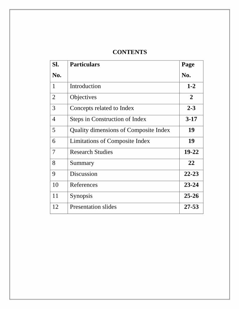
CONTENTS
Sl.
No.
Particulars Page
No.
1 Introduction 1-2
2 Objectives 2
3 Concepts related to Index 2-3
4 Steps in Construction of Index 3-17
5 Quality dimensions of Composite Index 19
6 Limitations of Composite Index 19
7 Research Studies 19-22
8 Summary 22
9 Discussion 22-23
10 References 23-24
11 Synopsis 25-26
12 Presentation slides 27-53
1
1. Introduction
The Social science research thrives to measure the human relations, behaviour, growth,
impact, comparative studies and many other socio-economic dimensions. It provides
substantial benefits to the communities at different levels i.e., local, regional, national and
international. The social science research can benefit to well being of the human mankind. The
social science can’t create the products but data that is useful for decisions. The output
information than the other forms. The ultimate aim is to produce the results that help in
improving the social and economic conditions. It initiates the institutional changes in
behavioural rules and governing pattern that establish larger social changes, life styles and way
of living. The demand for the knowledge leads the social science to more forward. The
movement of the benefits from social science move from individual, communities to the firms.
Social science research had brought many changes in more effective performance of household
or workplace (Smith, 1998).
The Agricultural Extension research merely consider as survey-based research. This
attitude that is formed on agricultural extension is more threatening for the existence of the
domain as discipline in research. There are several methods to conduct the studies on farmers
by taking methodologies from different disciplines. They include exploratory study,
explanatory study, participatory, scale development, index construction, case studies and many
more. The most valid Agricultural Extension research methodology includes the construction
of scale and composite index. The scale development is most common measurement technique
used by researchers and scholars of different social science domains. The other kind of
measurement composite index is collection of large number of indicators or variables that
aggregate to measure overall performance. It is increasingly recognised tool for policy
decisions.
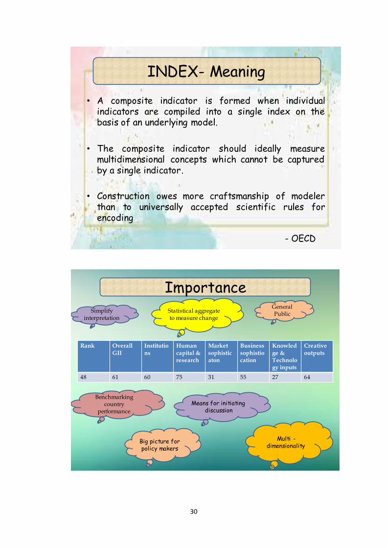
It became a means to start a discussion which ideally measures the multidimensional
concepts. The index development process statistically aggregates to measure the change. The
general public can understand the output of the composite index and interpret the same. It help
to bench mark the countries performance by comparing the trends with previous years. It also
facilitates in initiating the discussion by quoting the values to the composite index of a
particular country. It had greater importance to the policy makers. As the policymakers don’t
have time to discuss all the underlying aspect of a decision-making unit. It also serves as a
means to initiate discussion. The qualitative and the quantitative measure from the observed
facts that gives real relative position. The Google scholar search result from 2016 to 1st Dec.,
2020 gives 7,92,000 publications related to composite index depicts, how widely it is being
used.
A composite indicator or index is an aggregate of all dimensions, objectives, individual
indicators and variables used. This implies that what formally defines a composite indicator is
the set of properties underlying its aggregation convention. A composite indicator is formed
when individual indicators are compiled into a single index on the basis of an underlying
model. The composite indicator should ideally measure multidimensional concepts which
2
cannot be captured by a single indicator. Construction owes more craftsmanship of modeler
than to universally accepted scientific rules for encoding
The robustness of the index which is not thrown off by the random or partial variations.
It is able to distinguish between different cases. Efficient as it can be easy to build and measure.
The effectiveness of it depends on what exactly it captures. The robustness, discriminating,
efficient and effectiveness are the characteristics of an index. With this background, the present
seminar has been conceptualized with the following objectives:
2. Objectives
1. To know the concept of composite index
2. To understand different normalization, weighted and aggregation methods in composite
index construction
3. To review the related research studies
3. The Concepts related to Index
3.1 Objective:
It indicates the desired direction of change. For example, within the economic
dimension GDP has to be maximised; within the social dimension social exclusion has to be
minimised; within the environmental dimension CO2 emissions have to be minimised. This is
not always obvious: international mobility of researchers for example, could be minimized
when the hierarchical level is the country.
3.2 Indicator:
It is the basis for evaluation in relation to a given objective (any objective may imply a
number of different individual indicators). It is a function that associates each single country
with a variable indicating its desirability according to expected consequences related to the
same objective, e.g. GDP, saving rate and inflation rate within the objective “growth
maximisation”.
3.3 Dimension:
Dimension is the highest hierarchical level of analysis and indicates the scope of
objectives, individual indicators and variables. For example, a sustainability composite
indicator can include economic, social, environmental and institutional dimensions.
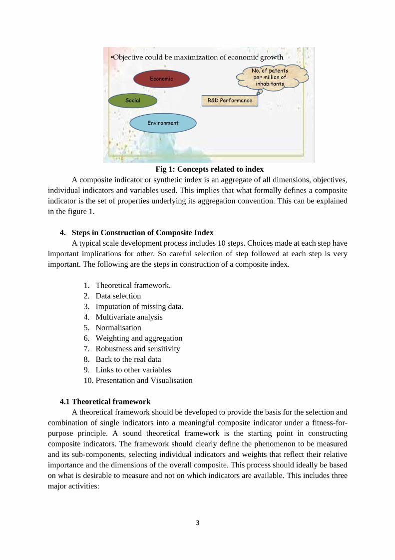
3.4 Variable:
It is a constructed measure stemming from a process that represents, at a given point in
space and time, a shared perception of a real-world state of affairs consistent with a given
individual indicator. For example, in comparing two countries within the economic dimension,
one objective could be “maximisation of economic growth”; the individual indicator might be
R&D performance, the indicator score or variable could be “number of patents per million of
inhabitants” as shown in the figure 1.
3
Fig 1: Concepts related to index
A composite indicator or synthetic index is an aggregate of all dimensions, objectives,
individual indicators and variables used. This implies that what formally defines a composite
indicator is the set of properties underlying its aggregation convention. This can be explained
in the figure 1.
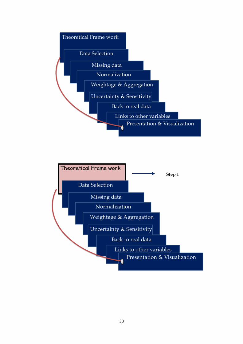
4. Steps in Construction of Composite Index
A typical scale development process includes 10 steps. Choices made at each step have
important implications for other. So careful selection of step followed at each step is very
important. The following are the steps in construction of a composite index.
1. Theoretical framework.
2. Data selection
3. Imputation of missing data.
4. Multivariate analysis
5. Normalisation
6. Weighting and aggregation
7. Robustness and sensitivity
8. Back to the real data
9. Links to other variables
10. Presentation and Visualisation
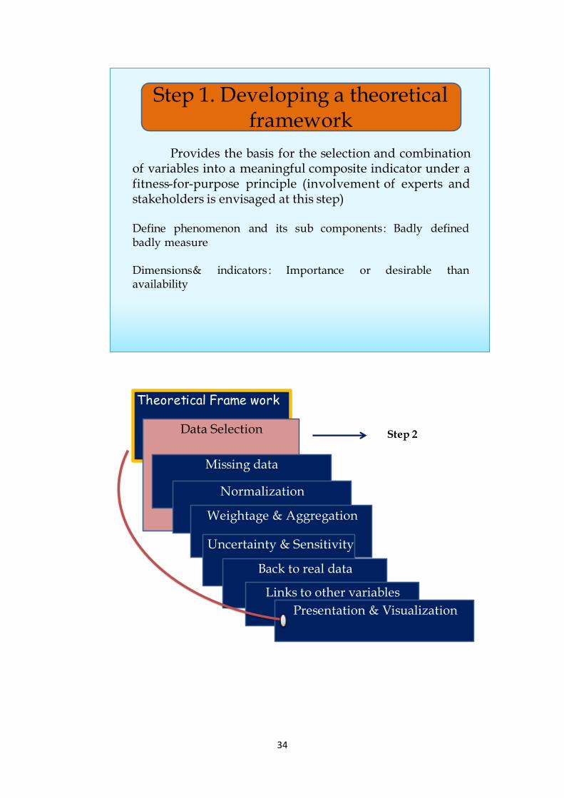
4.1 Theoretical framework
A theoretical framework should be developed to provide the basis for the selection and
combination of single indicators into a meaningful composite indicator under a fitness-for-
purpose principle. A sound theoretical framework is the starting point in constructing
composite indicators. The framework should clearly define the phenomenon to be measured
and its sub-components, selecting individual indicators and weights that reflect their relative
importance and the dimensions of the overall composite. This process should ideally be based
on what is desirable to measure and not on which indicators are available. This includes three
major activities:
4
4.1.1 Defining the concept
The definition should give the reader a clear sense of what is being measured by the
composite indicator. It should refer to the theoretical framework, linking various sub-groups
and the underlying indicators. Ultimately, the users of composite indicators should assess their
quality and relevance. In this both theoretical and operational definition included.
4.1.2 Determining sub-groups
Multi-dimensional concepts can be divided into several sub-groups. These sub-groups
need not be (statistically) independent of each other and existing linkages should be described
theoretically or empirically to the greatest extent possible. This step, as well as the next, should
involve experts and stakeholders as much as possible, in order to take into account multiple
viewpoints and to increase the robustness of the conceptual framework and set of indicators.
4.1.3 Identifying the selection criteria for the underlying indicators
The selection criteria should work as a guide to whether an indicator should be included
or not in the overall composite index. It should be as precise as possible and should describe
the phenomenon being measured.
4.1.4 By the end of this Step
• A clear understanding and definition of the multi-dimensional phenomenon to be measured.
• A nested structure of the various sub-groups of the phenomenon if needed.
• A list of selection criteria for the underlying variables, e.g. input, output, process.
• Clear documentation of the above
4.2 Data selection
Indicators should be selected on the basis of their analytical soundness, measurability,
country coverage, relevance to the phenomenon being measured and relationship to each other.
The use of proxy variables should be considered when data are scarce. The strengths and
weaknesses of composite indicators largely derive from the quality of the underlying variables.
Ideally, variables should be selected on the basis of their relevance, analytical soundness,
timeliness, accessibility, etc.
4.2.1 By the end of this Step
• Checked the quality of the available indicators.
• Discussed the strengths and weaknesses of each selected indicator.
• Created a summary table on data characteristics, e.g. availability (across country, time),
source, type (hard, soft or input, output, process).
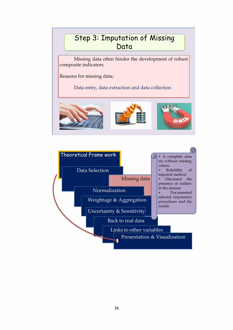
4.3 Imputation of missing data
Consideration should be given to different approaches for imputing missing values.
Extreme values should be examined as they can become unintended benchmarks. Missing data
often hinder the development of robust composite indicators. Data can be missing in a random
or non-random fashion. However, the reason for missing data starts with data collection, data
5
entry and data extraction during analysis. Three general methods for dealing with missing data
were three. In case deletion method the complete individual case will be deleted. The simple
imputation method only one imputation is used whereas multiple imputation method many
methods were used. The following are the missing data classification.
Missing completely at random (MCAR): Missing values do not depend on the
variable of interest or on any other observed variable in the data set
Missing at random (MAR): Missing values do not depend on the variable of interest,
but are conditional on other variables in the data set
Not missing at random (NMAR): Missing values depend on the values themselves.
For example, high income households are less likely to report their income.
4.3.1 By the end of this Step
• A complete data set without missing values.
• A measure of the reliability of each imputed value so as to explore the impact of imputation
on the composite indicator.
• Discussed the presence of outliers in the dataset
• Documented and explained the selected imputation procedures and the results.
4.4 Multivariate analysis
An exploratory analysis should investigate the overall structure of the indicators, assess
the suitability of the data set and explain the methodological choices, e.g. weighting,
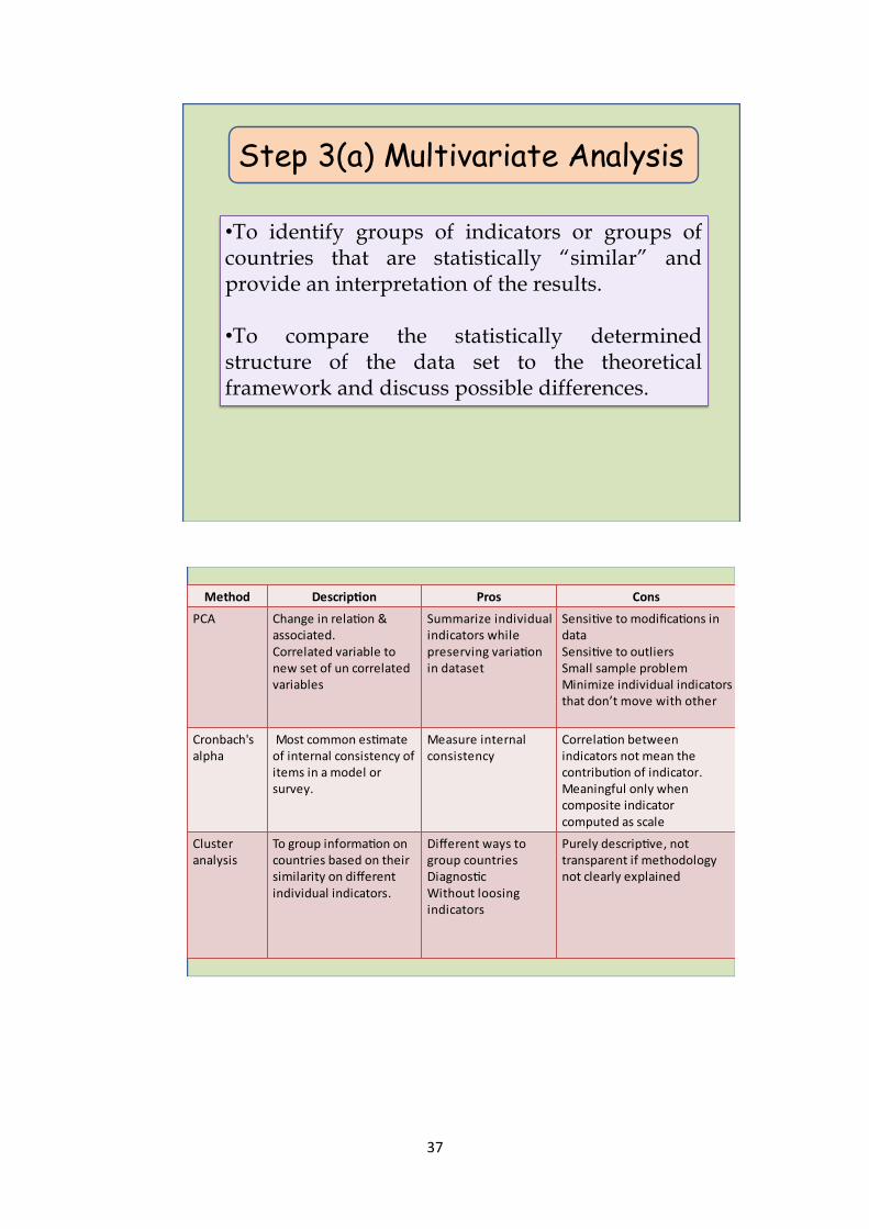
aggregation. To identify groups of indicators or groups of countries that are statistically
“similar” and provide an interpretation of the results. To compare the statistically determined
structure of the data set to the theoretical framework and discuss possible differences.
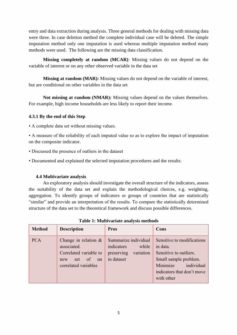
Table 1: Multivariate analysis methods
Method Description Pros Cons
PCA Change in relation &
associated.
Correlated variable to
new set of un
correlated variables
Summarize individual
indicators while
preserving variation
in dataset
Sensitive to modifications
in data.
Sensitive to outliers.
Small sample problem.
Minimize individual
indicators that don’t move
with other
6
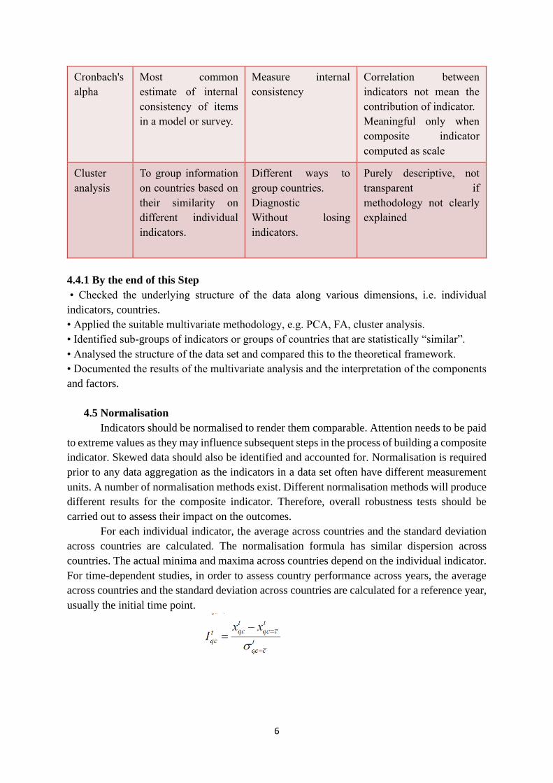
Cronbach's
alpha
Most common
estimate of internal
consistency of items
in a model or survey.
Measure internal
consistency
Correlation between
indicators not mean the
contribution of indicator.
Meaningful only when
composite indicator
computed as scale
Cluster
analysis
To group information
on countries based on
their similarity on
different individual
indicators.
Different ways to
group countries.
Diagnostic
Without losing
indicators.
Purely descriptive, not
transparent if
methodology not clearly
explained
4.4.1 By the end of this Step
• Checked the underlying structure of the data along various dimensions, i.e. individual
indicators, countries.
• Applied the suitable multivariate methodology, e.g. PCA, FA, cluster analysis.
• Identified sub-groups of indicators or groups of countries that are statistically “similar”.
• Analysed the structure of the data set and compared this to the theoretical framework.
• Documented the results of the multivariate analysis and the interpretation of the components
and factors.
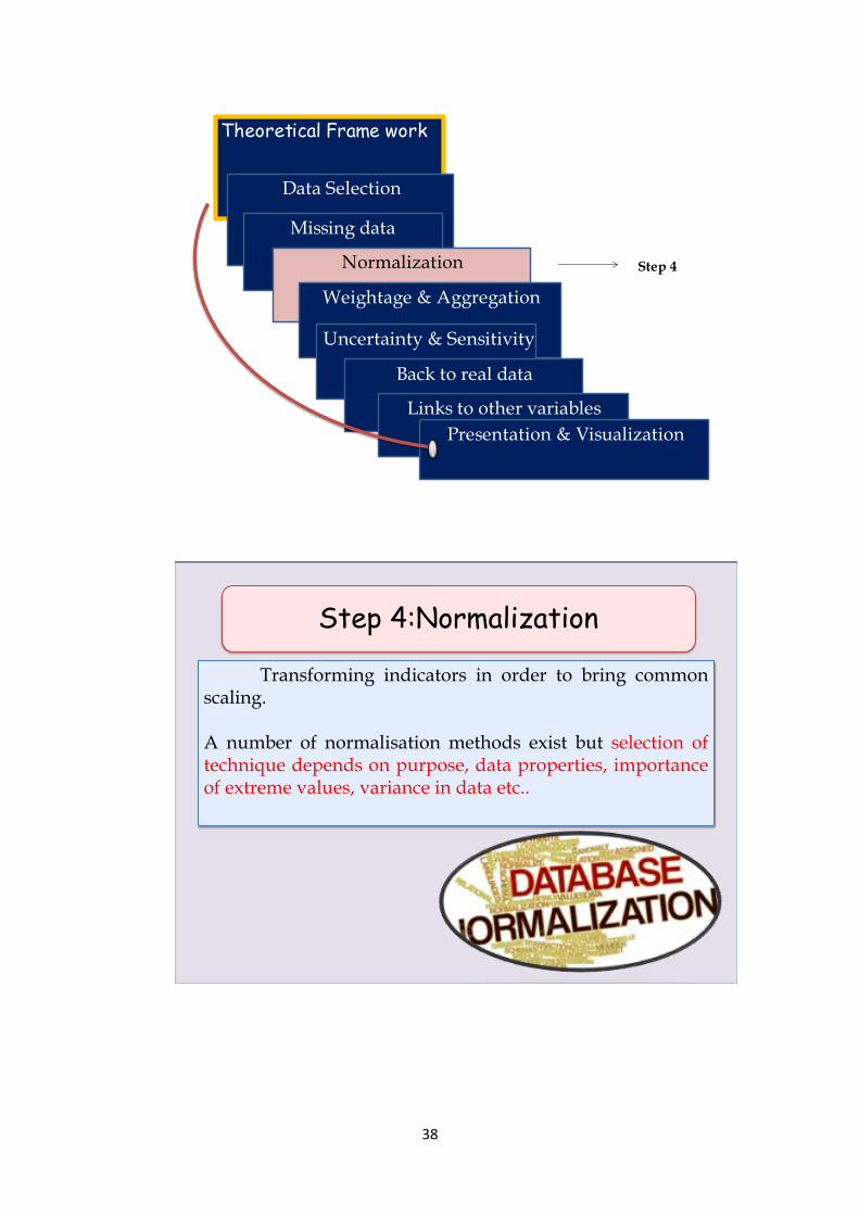
4.5 Normalisation
Indicators should be normalised to render them comparable. Attention needs to be paid
to extreme values as they may influence subsequent steps in the process of building a composite
indicator. Skewed data should also be identified and accounted for. Normalisation is required
prior to any data aggregation as the indicators in a data set often have different measurement
units. A number of normalisation methods exist. Different normalisation methods will produce
different results for the composite indicator. Therefore, overall robustness tests should be
carried out to assess their impact on the outcomes.
For each individual indicator, the average across countries and the standard deviation
across countries are calculated. The normalisation formula has similar dispersion across
countries. The actual minima and maxima across countries depend on the individual indicator.
For time-dependent studies, in order to assess country performance across years, the average
across countries and the standard deviation across countries are calculated for a reference year,
usually the initial time point.
7
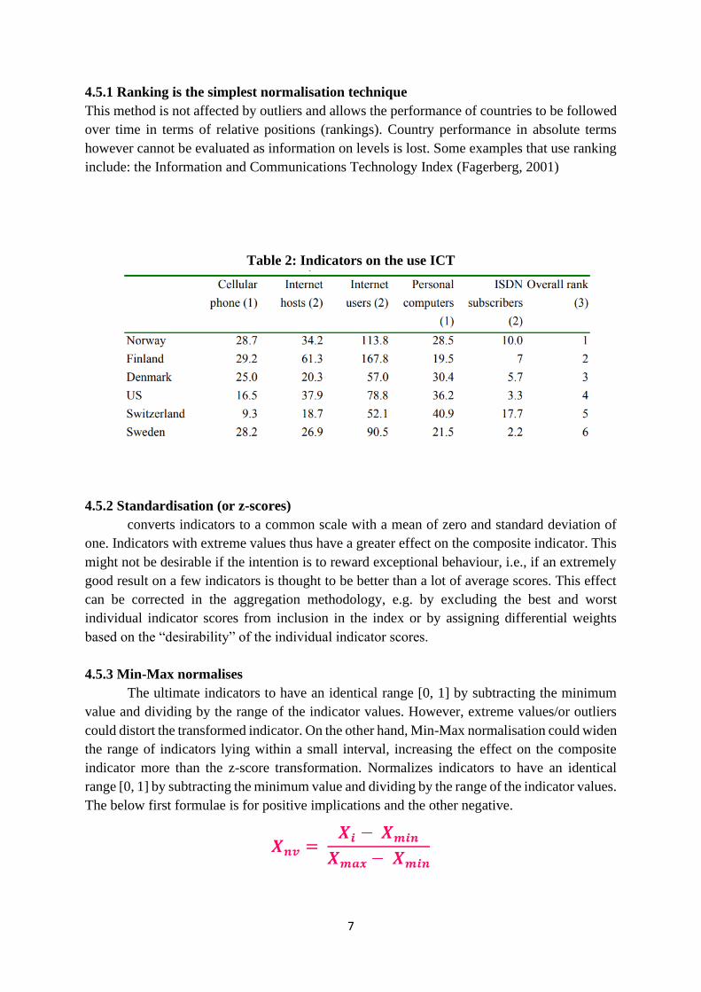
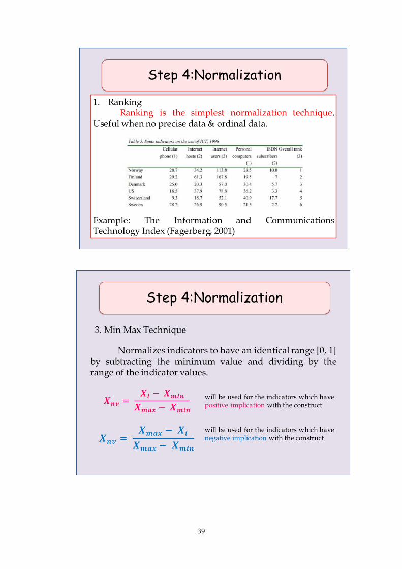
4.5.1 Ranking is the simplest normalisation technique
This method is not affected by outliers and allows the performance of countries to be followed
over time in terms of relative positions (rankings). Country performance in absolute terms
however cannot be evaluated as information on levels is lost. Some examples that use ranking
include: the Information and Communications Technology Index (Fagerberg, 2001)
Table 2: Indicators on the use ICT
4.5.2 Standardisation (or z-scores)
converts indicators to a common scale with a mean of zero and standard deviation of
one. Indicators with extreme values thus have a greater effect on the composite indicator. This
might not be desirable if the intention is to reward exceptional behaviour, i.e., if an extremely
good result on a few indicators is thought to be better than a lot of average scores. This effect
can be corrected in the aggregation methodology, e.g. by excluding the best and worst
individual indicator scores from inclusion in the index or by assigning differential weights
based on the “desirability” of the individual indicator scores.
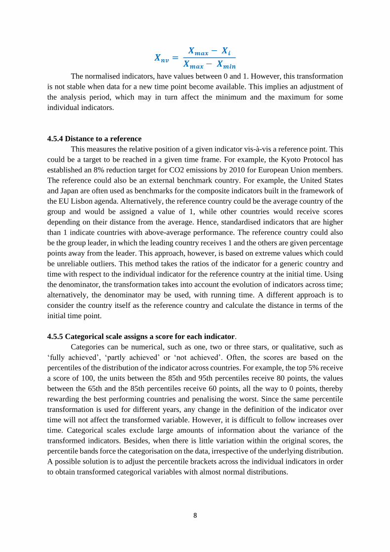
4.5.3 Min-Max normalises
The ultimate indicators to have an identical range [0, 1] by subtracting the minimum
value and dividing by the range of the indicator values. However, extreme values/or outliers
could distort the transformed indicator. On the other hand, Min-Max normalisation could widen
the range of indicators lying within a small interval, increasing the effect on the composite
indicator more than the z-score transformation. Normalizes indicators to have an identical
range [0, 1] by subtracting the minimum value and dividing by the range of the indicator values.
The below first formulae is for positive implications and the other negative.
8
The normalised indicators, have values between 0 and 1. However, this transformation
is not stable when data for a new time point become available. This implies an adjustment of
the analysis period, which may in turn affect the minimum and the maximum for some
individual indicators.
4.5.4 Distance to a reference
This measures the relative position of a given indicator vis-à-vis a reference point. This
could be a target to be reached in a given time frame. For example, the Kyoto Protocol has
established an 8% reduction target for CO2 emissions by 2010 for European Union members.
The reference could also be an external benchmark country. For example, the United States
and Japan are often used as benchmarks for the composite indicators built in the framework of
the EU Lisbon agenda. Alternatively, the reference country could be the average country of the
group and would be assigned a value of 1, while other countries would receive scores
depending on their distance from the average. Hence, standardised indicators that are higher
than 1 indicate countries with above-average performance. The reference country could also
be the group leader, in which the leading country receives 1 and the others are given percentage
points away from the leader. This approach, however, is based on extreme values which could
be unreliable outliers. This method takes the ratios of the indicator for a generic country and
time with respect to the individual indicator for the reference country at the initial time. Using
the denominator, the transformation takes into account the evolution of indicators across time;
alternatively, the denominator may be used, with running time. A different approach is to
consider the country itself as the reference country and calculate the distance in terms of the
initial time point.
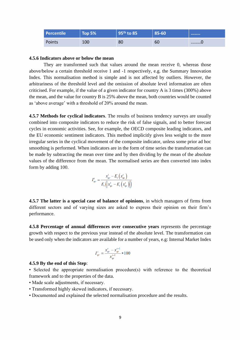
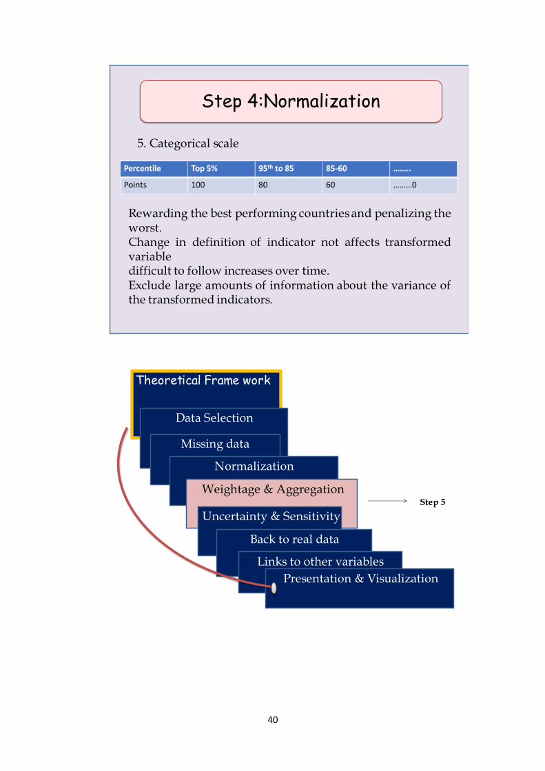
4.5.5 Categorical scale assigns a score for each indicator.
Categories can be numerical, such as one, two or three stars, or qualitative, such as
‘fully achieved’, ‘partly achieved’ or ‘not achieved’. Often, the scores are based on the
percentiles of the distribution of the indicator across countries. For example, the top 5% receive
a score of 100, the units between the 85th and 95th percentiles receive 80 points, the values
between the 65th and the 85th percentiles receive 60 points, all the way to 0 points, thereby
rewarding the best performing countries and penalising the worst. Since the same percentile
transformation is used for different years, any change in the definition of the indicator over
time will not affect the transformed variable. However, it is difficult to follow increases over
time. Categorical scales exclude large amounts of information about the variance of the
transformed indicators. Besides, when there is little variation within the original scores, the
percentile bands force the categorisation on the data, irrespective of the underlying distribution.
A possible solution is to adjust the percentile brackets across the individual indicators in order
to obtain transformed categorical variables with almost normal distributions.
9
4.5.6 Indicators above or below the mean
They are transformed such that values around the mean receive 0, whereas those
above/below a certain threshold receive 1 and -1 respectively, e.g. the Summary Innovation
Index. This normalisation method is simple and is not affected by outliers. However, the
arbitrariness of the threshold level and the omission of absolute level information are often
criticised. For example, if the value of a given indicator for country A is 3 times (300%) above
the mean, and the value for country B is 25% above the mean, both countries would be counted
as ‘above average’ with a threshold of 20% around the mean.
4.5.7 Methods for cyclical indicators. The results of business tendency surveys are usually
combined into composite indicators to reduce the risk of false signals, and to better forecast
cycles in economic activities. See, for example, the OECD composite leading indicators, and
the EU economic sentiment indicators. This method implicitly gives less weight to the more
irregular series in the cyclical movement of the composite indicator, unless some prior ad hoc
smoothing is performed. When indicators are in the form of time series the transformation can
be made by subtracting the mean over time and by then dividing by the mean of the absolute
values of the difference from the mean. The normalised series are then converted into index
form by adding 100.
4.5.7 The latter is a special case of balance of opinions, in which managers of firms from
different sectors and of varying sizes are asked to express their opinion on their firm’s
performance.
4.5.8 Percentage of annual differences over consecutive years represents the percentage
growth with respect to the previous year instead of the absolute level. The transformation can
be used only when the indicators are available for a number of years, e.g: Internal Market Index
4.5.9 By the end of this Step:
• Selected the appropriate normalisation procedure(s) with reference to the theoretical
framework and to the properties of the data.
• Made scale adjustments, if necessary.
• Transformed highly skewed indicators, if necessary.
• Documented and explained the selected normalisation procedure and the results.
10
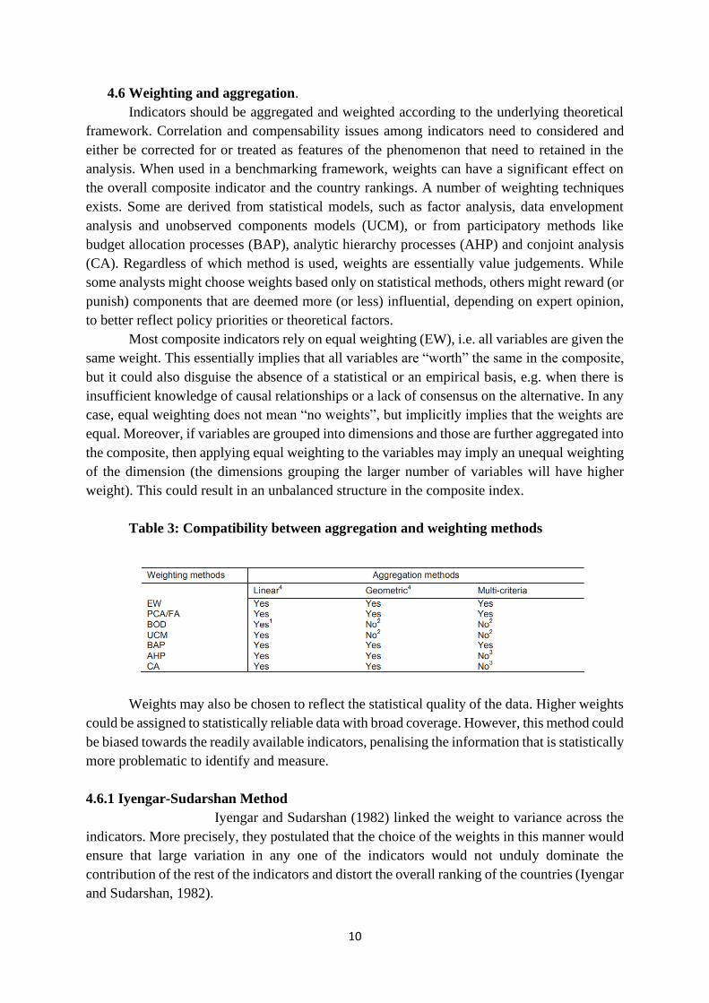
4.6 Weighting and aggregation.
Indicators should be aggregated and weighted according to the underlying theoretical
framework. Correlation and compensability issues among indicators need to considered and
either be corrected for or treated as features of the phenomenon that need to retained in the
analysis. When used in a benchmarking framework, weights can have a significant effect on
the overall composite indicator and the country rankings. A number of weighting techniques
exists. Some are derived from statistical models, such as factor analysis, data envelopment
analysis and unobserved components models (UCM), or from participatory methods like
budget allocation processes (BAP), analytic hierarchy processes (AHP) and conjoint analysis
(CA). Regardless of which method is used, weights are essentially value judgements. While
some analysts might choose weights based only on statistical methods, others might reward (or
punish) components that are deemed more (or less) influential, depending on expert opinion,
to better reflect policy priorities or theoretical factors.
Most composite indicators rely on equal weighting (EW), i.e. all variables are given the
same weight. This essentially implies that all variables are “worth” the same in the composite,
but it could also disguise the absence of a statistical or an empirical basis, e.g. when there is
insufficient knowledge of causal relationships or a lack of consensus on the alternative. In any
case, equal weighting does not mean “no weights”, but implicitly implies that the weights are
equal. Moreover, if variables are grouped into dimensions and those are further aggregated into
the composite, then applying equal weighting to the variables may imply an unequal weighting
of the dimension (the dimensions grouping the larger number of variables will have higher
weight). This could result in an unbalanced structure in the composite index.
Table 3: Compatibility between aggregation and weighting methods
Weights may also be chosen to reflect the statistical quality of the data. Higher weights
could be assigned to statistically reliable data with broad coverage. However, this method could
be biased towards the readily available indicators, penalising the information that is statistically
more problematic to identify and measure.
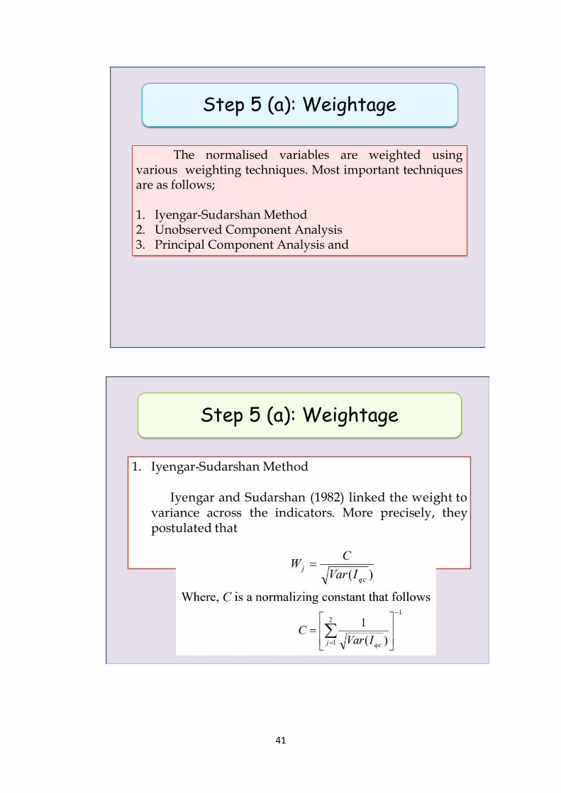
4.6.1 Iyengar-Sudarshan Method
Iyengar and Sudarshan (1982) linked the weight to variance across the
indicators. More precisely, they postulated that the choice of the weights in this manner would
ensure that large variation in any one of the indicators would not unduly dominate the
contribution of the rest of the indicators and distort the overall ranking of the countries (Iyengar
and Sudarshan, 1982).
11
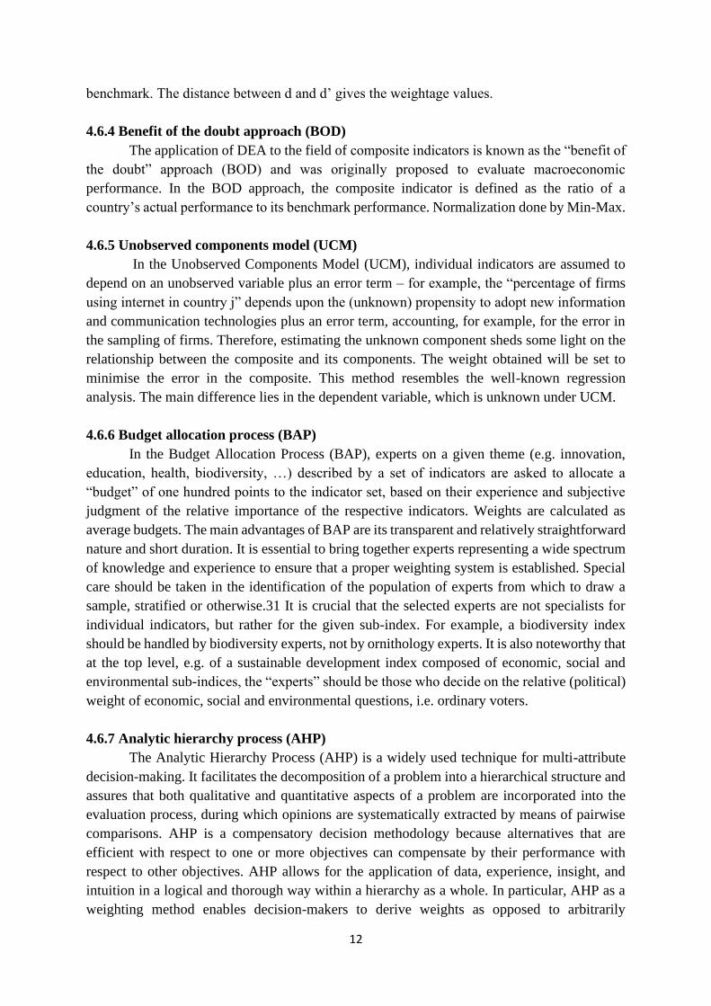
4.6.2 PCA
Principal components analysis, and more specifically factor analysis, groups together
individual indicators which are collinear to form a composite indicator that captures as much
as possible of the information common to individual indicators. Note that individual indicators
must have the same unit of measurement. Each factor (usually estimated using principal
components analysis) reveals the set of indicators with which it has the strongest association.
The idea under PCA/FA is to account for the highest possible variation in the indicator set
using the smallest possible number of factors. Therefore, the composite no longer depends
upon the dimensionality of the data set but rather is based on the “statistical” dimensions of the
data.
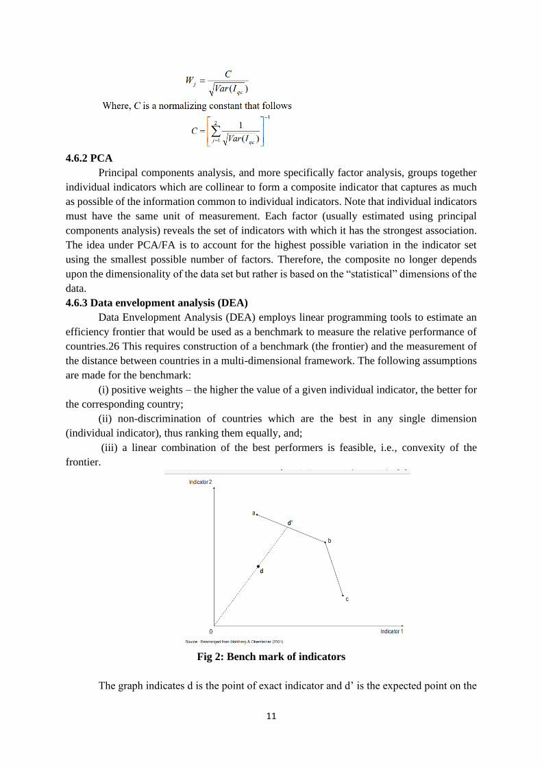
4.6.3 Data envelopment analysis (DEA)
Data Envelopment Analysis (DEA) employs linear programming tools to estimate an
efficiency frontier that would be used as a benchmark to measure the relative performance of
countries.26 This requires construction of a benchmark (the frontier) and the measurement of
the distance between countries in a multi-dimensional framework. The following assumptions
are made for the benchmark:
(i) positive weights – the higher the value of a given individual indicator, the better for
the corresponding country;
(ii) non-discrimination of countries which are the best in any single dimension
(individual indicator), thus ranking them equally, and;
(iii) a linear combination of the best performers is feasible, i.e., convexity of the
frontier.
Fig 2: Bench mark of indicators
The graph indicates d is the point of exact indicator and d’ is the expected point on the
12
benchmark. The distance between d and d’ gives the weightage values.
4.6.4 Benefit of the doubt approach (BOD)
The application of DEA to the field of composite indicators is known as the “benefit of
the doubt” approach (BOD) and was originally proposed to evaluate macroeconomic
performance. In the BOD approach, the composite indicator is defined as the ratio of a
country’s actual performance to its benchmark performance. Normalization done by Min-Max.
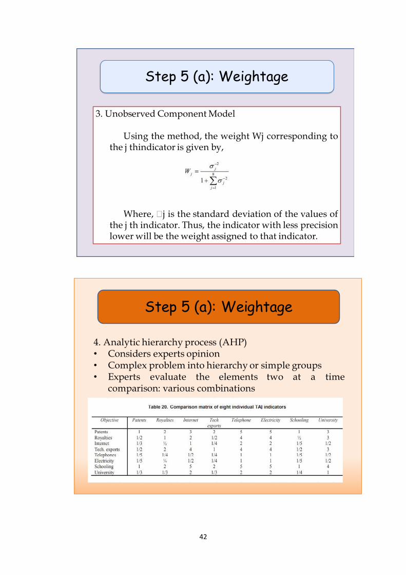
4.6.5 Unobserved components model (UCM)
In the Unobserved Components Model (UCM), individual indicators are assumed to
depend on an unobserved variable plus an error term – for example, the “percentage of firms
using internet in country j” depends upon the (unknown) propensity to adopt new information
and communication technologies plus an error term, accounting, for example, for the error in
the sampling of firms. Therefore, estimating the unknown component sheds some light on the
relationship between the composite and its components. The weight obtained will be set to
minimise the error in the composite. This method resembles the well-known regression
analysis. The main difference lies in the dependent variable, which is unknown under UCM.
4.6.6 Budget allocation process (BAP)
In the Budget Allocation Process (BAP), experts on a given theme (e.g. innovation,
education, health, biodiversity, …) described by a set of indicators are asked to allocate a
“budget” of one hundred points to the indicator set, based on their experience and subjective
judgment of the relative importance of the respective indicators. Weights are calculated as
average budgets. The main advantages of BAP are its transparent and relatively straightforward
nature and short duration. It is essential to bring together experts representing a wide spectrum
of knowledge and experience to ensure that a proper weighting system is established. Special
care should be taken in the identification of the population of experts from which to draw a
sample, stratified or otherwise.31 It is crucial that the selected experts are not specialists for
individual indicators, but rather for the given sub-index. For example, a biodiversity index
should be handled by biodiversity experts, not by ornithology experts. It is also noteworthy that
at the top level, e.g. of a sustainable development index composed of economic, social and
environmental sub-indices, the “experts” should be those who decide on the relative (political)
weight of economic, social and environmental questions, i.e. ordinary voters.
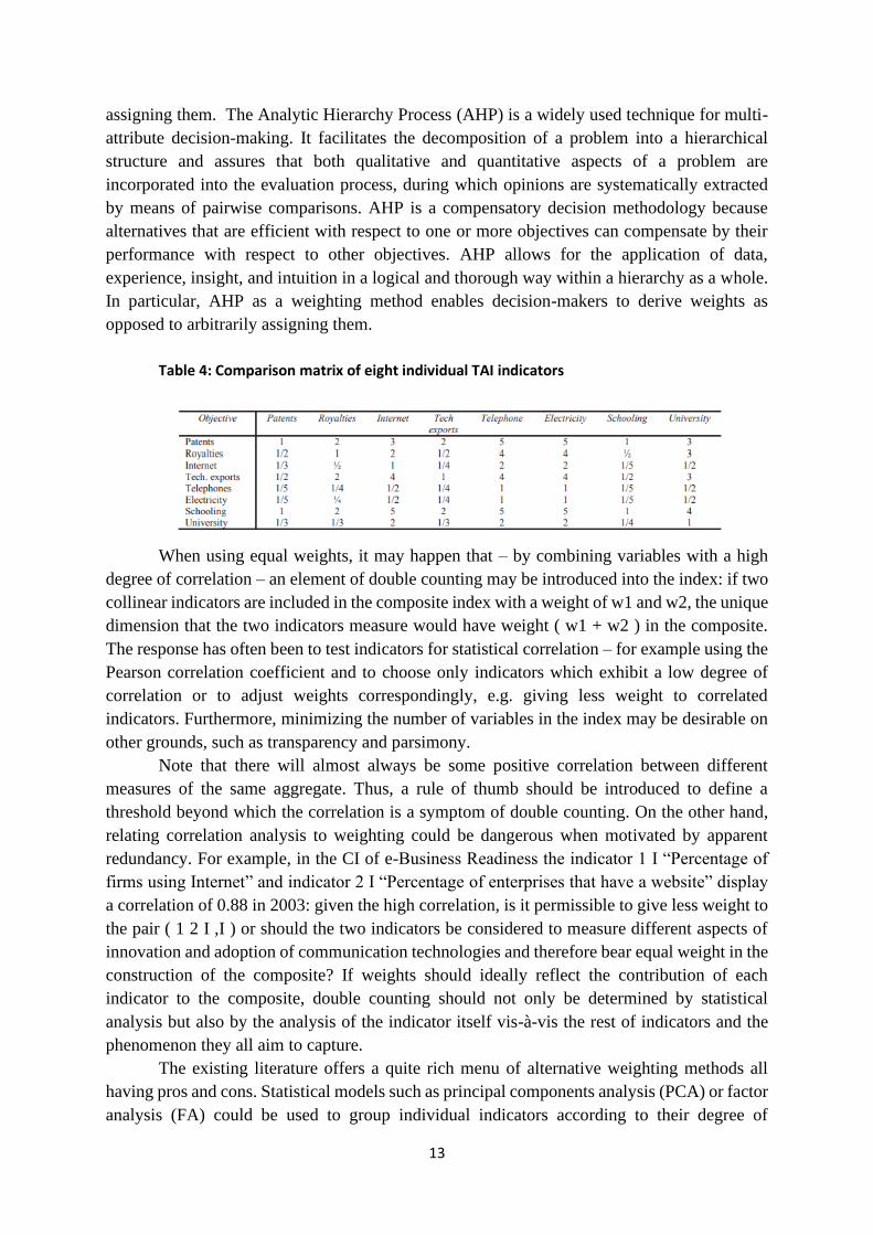
4.6.7 Analytic hierarchy process (AHP)
The Analytic Hierarchy Process (AHP) is a widely used technique for multi-attribute
decision-making. It facilitates the decomposition of a problem into a hierarchical structure and
assures that both qualitative and quantitative aspects of a problem are incorporated into the
evaluation process, during which opinions are systematically extracted by means of pairwise
comparisons. AHP is a compensatory decision methodology because alternatives that are
efficient with respect to one or more objectives can compensate by their performance with
respect to other objectives. AHP allows for the application of data, experience, insight, and
intuition in a logical and thorough way within a hierarchy as a whole. In particular, AHP as a
weighting method enables decision-makers to derive weights as opposed to arbitrarily
13
assigning them. The Analytic Hierarchy Process (AHP) is a widely used technique for multi-
attribute decision-making. It facilitates the decomposition of a problem into a hierarchical
structure and assures that both qualitative and quantitative aspects of a problem are
incorporated into the evaluation process, during which opinions are systematically extracted
by means of pairwise comparisons. AHP is a compensatory decision methodology because
alternatives that are efficient with respect to one or more objectives can compensate by their
performance with respect to other objectives. AHP allows for the application of data,
experience, insight, and intuition in a logical and thorough way within a hierarchy as a whole.
In particular, AHP as a weighting method enables decision-makers to derive weights as
opposed to arbitrarily assigning them.
Table 4: Comparison matrix of eight individual TAI indicators
When using equal weights, it may happen that – by combining variables with a high
degree of correlation – an element of double counting may be introduced into the index: if two
collinear indicators are included in the composite index with a weight of w1 and w2, the unique
dimension that the two indicators measure would have weight ( w1 + w2 ) in the composite.
The response has often been to test indicators for statistical correlation – for example using the
Pearson correlation coefficient and to choose only indicators which exhibit a low degree of
correlation or to adjust weights correspondingly, e.g. giving less weight to correlated
indicators. Furthermore, minimizing the number of variables in the index may be desirable on
other grounds, such as transparency and parsimony.
Note that there will almost always be some positive correlation between different
measures of the same aggregate. Thus, a rule of thumb should be introduced to define a
threshold beyond which the correlation is a symptom of double counting. On the other hand,
relating correlation analysis to weighting could be dangerous when motivated by apparent
redundancy. For example, in the CI of e-Business Readiness the indicator 1 I “Percentage of
firms using Internet” and indicator 2 I “Percentage of enterprises that have a website” display
a correlation of 0.88 in 2003: given the high correlation, is it permissible to give less weight to
the pair ( 1 2 I ,I ) or should the two indicators be considered to measure different aspects of
innovation and adoption of communication technologies and therefore bear equal weight in the
construction of the composite? If weights should ideally reflect the contribution of each
indicator to the composite, double counting should not only be determined by statistical
analysis but also by the analysis of the indicator itself vis-à-vis the rest of indicators and the
phenomenon they all aim to capture.
The existing literature offers a quite rich menu of alternative weighting methods all
having pros and cons. Statistical models such as principal components analysis (PCA) or factor
analysis (FA) could be used to group individual indicators according to their degree of
14
correlation. Weights, however, cannot be estimated with these methods if no correlation exists
between indicators. Other statistical methods, such as the “benefit of the doubt” (BOD)
approach, are extremely parsimonious about weighting assumptions as they allow the data to
decide on the weights and are sensitive to national priorities. However, with BOD weights are
country specific and have a number of estimation problems.
Alternatively, participatory methods that incorporate various stakeholders – experts,
citizens and politicians – can be used to assign weights. This approach is feasible when there
is a well-defined basis for a national policy. For international comparisons, such references are
often not available, or deliver contradictory results. In the budget allocation approach, experts
are given a “budget” of N points, to be distributed over a number of individual indicators,
“paying” more for those indicators whose importance they want to stress. The budget allocation
is optimal for a maximum of 10-12 indicators. If too many indicators are involved, this method
can induce serious cognitive stress in the experts who are asked to allocate the budget. Public
opinion polls have been extensively used over the years as they are easy and inexpensive to
carry out.
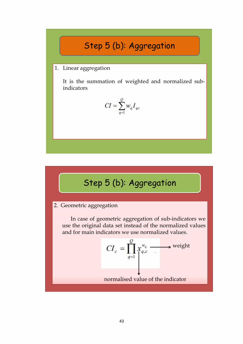
4.6 b. Aggregation
Aggregation methods also vary. While the linear aggregation method is useful when all
individual indicators have the same measurement unit, provided that some mathematical
properties are respected. Geometric aggregations are better suited if the modeller wants some
degree of non-compensability between individual indicators or dimensions. Furthermore,
linear aggregations reward base-indicators proportionally to the weights, while geometric
aggregations reward those countries with higher scores.
In both linear and geometric aggregations, weights express trade-offs between
indicators. A deficit in one dimension can thus be offset (compensated) by a surplus in another.
This implies an inconsistency between how weights are conceived (usually measuring the
importance of the associated variable) and the actual meaning when geometric or linear
aggregations are used. In a linear aggregation, the compensability is constant, while with
geometric aggregations compensability is lower for the composite indicators with low values.
In terms of policy, if compensability is admitted (as in the case of pure economic indicators),
a country with low scores on one indicator will need a much higher score on the others to
improve its situation when geometric aggregation is used. Thus, in benchmarking exercises,
countries with low scores prefer a linear rather than a geometric aggregation. On the other hand,
the marginal utility from an increase in low absolute score would be much higher than in a high
absolute score under geometric aggregation. Consequently, a country would have a greater
incentive to address those sectors/activities/alternatives with low scores if the aggregation were
geometric rather than linear, as this would give it a better chance of improving its position in
the ranking.
To ensure that weights remain a measure of importance, other aggregation methods
should be used, in particular methods that do not allow compensability. Moreover, if different
goals are equally legitimate and important, a non-compensatory logic might be necessary. This
is usually the case when highly different dimensions are aggregated in the composite, as in the
case of environmental indices that include physical, social and economic data. If the analyst
decides that an increase in economic performance cannot compensate for a loss in social

15
cohesion or a worsening in environmental sustainability, then neither the linear nor the
geometric aggregation is suitable. A non-compensatory multi-criteria approach (MCA) could
assure non-compensability by finding a compromise between two or more legitimate goals. In
its basic form this approach does not reward outliers, as it retains only ordinal information, i.e.
those countries having a greater advantage (disadvantage) in individual indicators. This
method, however, could be computationally costly when the number of countries is high, as
the number of permutations to calculate increases exponentially.
Table 5: Composite Indices Formed by Linear Aggregation Method Using
Different Weighting Techniques
16
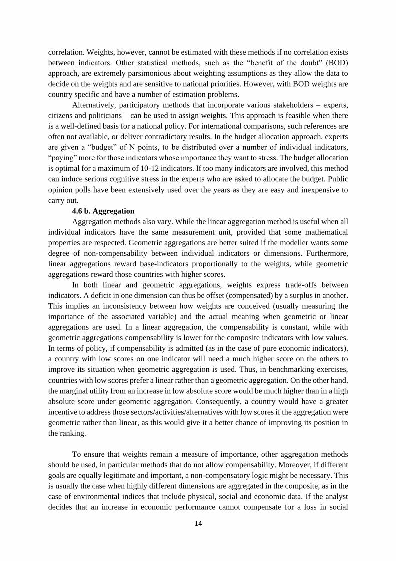
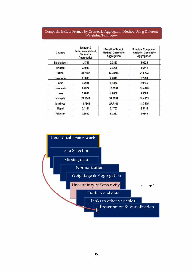
Table 6: Composite Indices Formed by Geometric Aggregation Method Using
Different Weighting Techniques
The table 5 and 6 determine how the different values changes with the linear and
geometric methods of aggregation in different weightage methods.
With regard to the time element, keeping weights unchanged across time might be
justified if the researcher is willing to analyse the evolution of a certain number of variables,
as in the case of the evolution of the EC Internal Market Index from 1992 to 2002. Weights do
not change with MCA, being associated to the intrinsic value of the indicators used to explain
the phenomenon. If, instead, the objective of the analysis is that of defining best practice or of
setting priorities, then weights should necessarily change over time.
The absence of an “objective” way to determine weights and aggregation methods does
not necessarily lead to rejection of the validity of composite indicators, as long as the entire
process is transparent. The modeller’s objectives must be clearly stated at the outset, and the
chosen model must be tested to see to what extent it fulfils the modeller’s goal.
4.6.8 By the end of this Step
• Selected the appropriate weighting and aggregation procedure(s) with reference to the
theoretical framework.
• Considered the possibility of using alternative methods (multi-modelling principle).
• Discussed whether correlation issues among indicators should be accounted for
• Discussed whether compensability among indicators should be allowed • Documented and
explained the weighting and aggregation procedures selected.
17
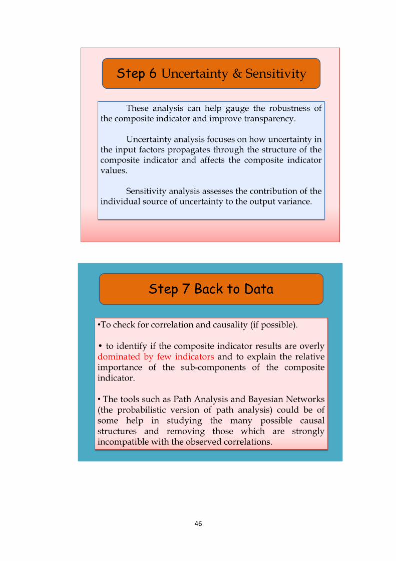
4.7 Robustness and sensitivity.
Analysis should be undertaken to assess the robustness of the composite indicator in
terms of, e.g., the mechanism for including or excluding single indicators, the normalisation
scheme, the imputation of missing data, the choice of weights and the aggregation method.
Several judgements have to be made when constructing composite indicators, e.g., on the
selection of indicators, data normalisation, weights and aggregation methods, etc. The
robustness of the composite indicators and the underlying policy messages may thus be
contested. A combination of uncertainty and sensitivity analysis can help gauge the robustness
of the composite indicator and improve transparency.
4.7.1 By the end of this Step
• Identified the sources of uncertainty in the development of the composite indicator.
• Assessed the impact of the uncertainties/assumptions on the final result.
• Conducted sensitivity analysis of the inference, e.g. to show what sources of uncertainty are
more influential in determining the relative ranking of two entities.
• Documented and explained the sensitivity analyses and the results.
4.8 Back to the real data.
Composite indicators should be transparent and fit to be decomposed into their
underlying indicators or values. Composite indicators provide a starting point for analysis.
While they can be used as summary indicators to guide policy and data work, they can also be
decomposed such that the contribution of subcomponents and individual indicators can be
identified and the analysis of country performance extended.
4.8.1 By the end of this Step
• Decomposed the composite indicator into its individual parts and tested for correlation and
causality (if possible).
• Profiled country performance at the indicator level to reveal what is driving the composite
indicator results, and in particular whether the composite indicator is overly dominated by a
small number of indicators.
• Documented and explained the relative importance of the sub-components of the composite
indicator.
4.9 Links to other variables.
Attempts should be made to correlate the composite indicator with other published
indicators, as well as to identify linkages through regressions. Composite indicators often
measure concepts that are linked to well-known and measurable phenomena, e.g. productivity
growth, entry of new firms. These links can be used to test the explanatory power of a
composite. Simple cross-plots are often the best way to illustrate such links. An indicator
measuring the environment for business start-ups, for example, could be linked to entry rates
of new firms, where good performance on the composite indicator of business environment
would be expected to yield higher entry rates.
18
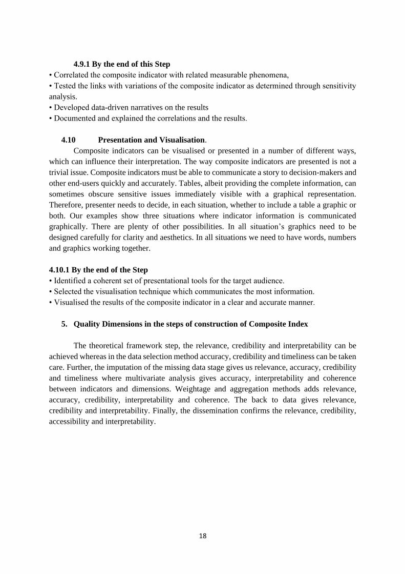
4.9.1 By the end of this Step
• Correlated the composite indicator with related measurable phenomena,
• Tested the links with variations of the composite indicator as determined through sensitivity
analysis.
• Developed data-driven narratives on the results
• Documented and explained the correlations and the results.
4.10 Presentation and Visualisation.
Composite indicators can be visualised or presented in a number of different ways,
which can influence their interpretation. The way composite indicators are presented is not a
trivial issue. Composite indicators must be able to communicate a story to decision-makers and
other end-users quickly and accurately. Tables, albeit providing the complete information, can
sometimes obscure sensitive issues immediately visible with a graphical representation.
Therefore, presenter needs to decide, in each situation, whether to include a table a graphic or
both. Our examples show three situations where indicator information is communicated
graphically. There are plenty of other possibilities. In all situation’s graphics need to be
designed carefully for clarity and aesthetics. In all situations we need to have words, numbers
and graphics working together.
4.10.1 By the end of the Step
• Identified a coherent set of presentational tools for the target audience.
• Selected the visualisation technique which communicates the most information.
• Visualised the results of the composite indicator in a clear and accurate manner.
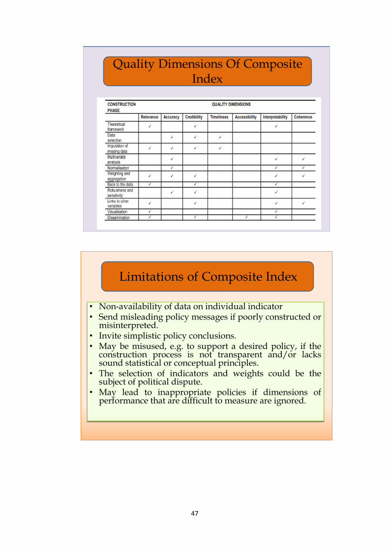
5. Quality Dimensions in the steps of construction of Composite Index
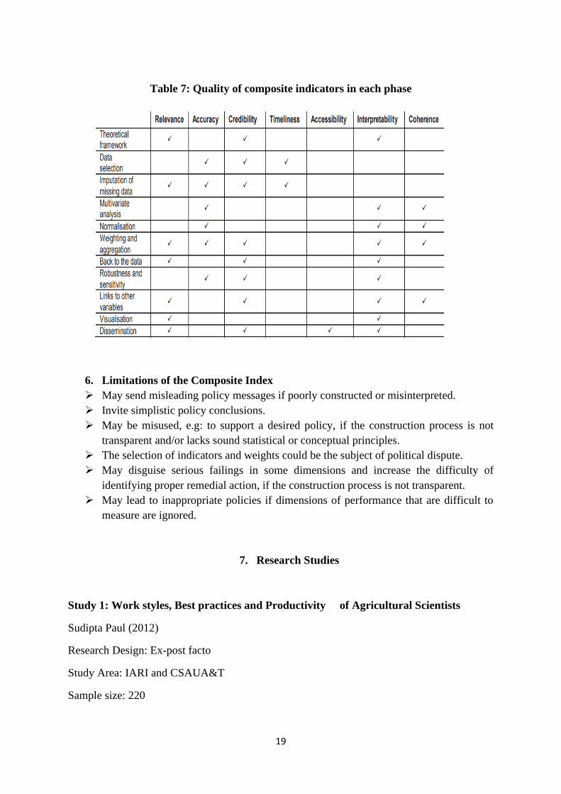
The theoretical framework step, the relevance, credibility and interpretability can be
achieved whereas in the data selection method accuracy, credibility and timeliness can be taken
care. Further, the imputation of the missing data stage gives us relevance, accuracy, credibility
and timeliness where multivariate analysis gives accuracy, interpretability and coherence
between indicators and dimensions. Weightage and aggregation methods adds relevance,
accuracy, credibility, interpretability and coherence. The back to data gives relevance,
credibility and interpretability. Finally, the dissemination confirms the relevance, credibility,
accessibility and interpretability.
19
Table 7: Quality of composite indicators in each phase
6. Limitations of the Composite Index
➢ May send misleading policy messages if poorly constructed or misinterpreted.
➢ Invite simplistic policy conclusions.
➢ May be misused, e.g: to support a desired policy, if the construction process is not
transparent and/or lacks sound statistical or conceptual principles.
➢ The selection of indicators and weights could be the subject of political dispute.
➢ May disguise serious failings in some dimensions and increase the difficulty of
identifying proper remedial action, if the construction process is not transparent.
➢ May lead to inappropriate policies if dimensions of performance that are difficult to
measure are ignored.
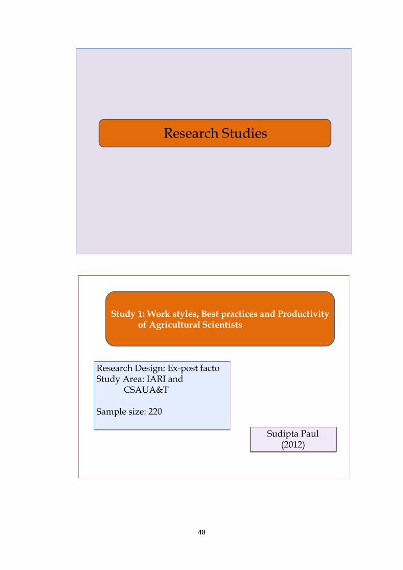
7. Research Studies
Study 1: Work styles, Best practices and Productivity of Agricultural Scientists
Sudipta Paul (2012)
Research Design: Ex-post facto
Study Area: IARI and CSAUA&T
Sample size: 220
20
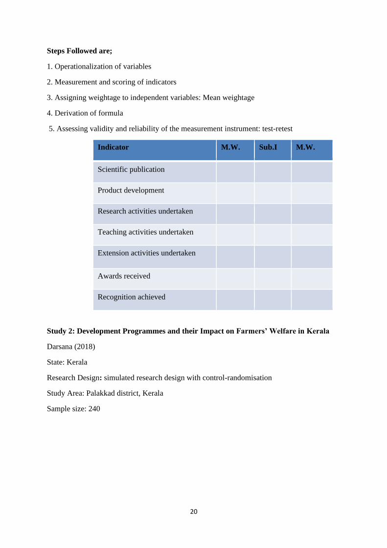
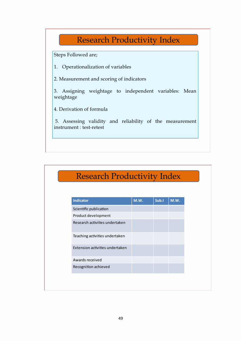
Steps Followed are;
1. Operationalization of variables
2. Measurement and scoring of indicators
3. Assigning weightage to independent variables: Mean weightage
4. Derivation of formula
5. Assessing validity and reliability of the measurement instrument: test-retest
Indicator M.W. Sub.I M.W.
Scientific publication
Product development
Research activities undertaken
Teaching activities undertaken
Extension activities undertaken
Awards received
Recognition achieved
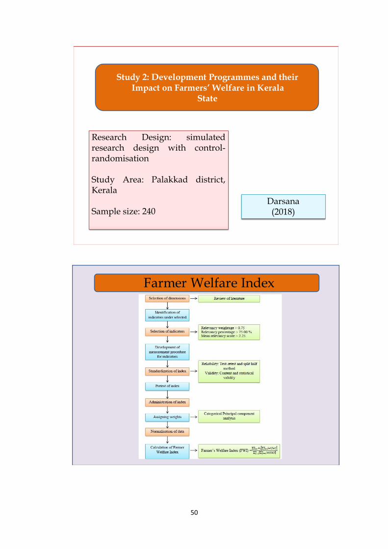
Study 2: Development Programmes and their Impact on Farmers’ Welfare in Kerala
Darsana (2018)
State: Kerala
Research Design: simulated research design with control-randomisation
Study Area: Palakkad district, Kerala
Sample size: 240
21
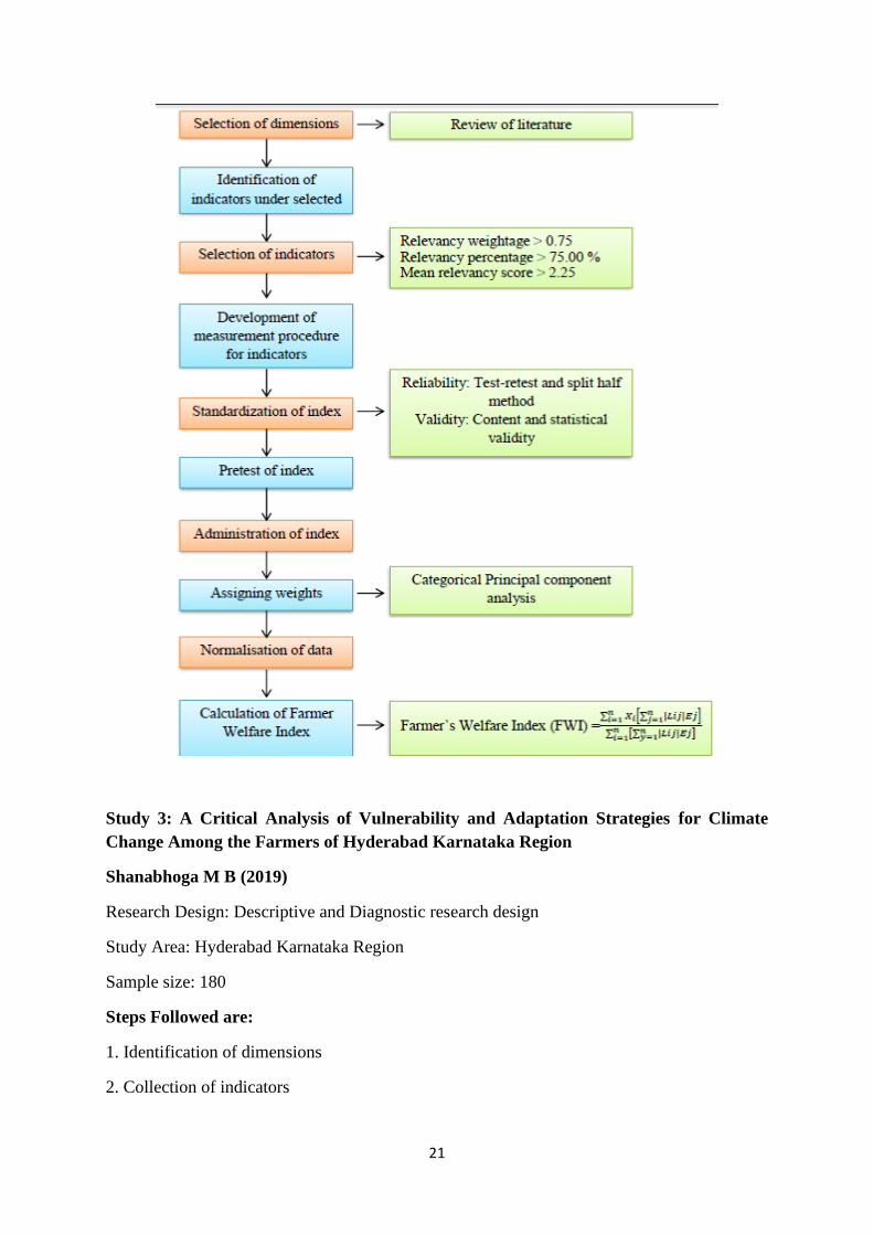
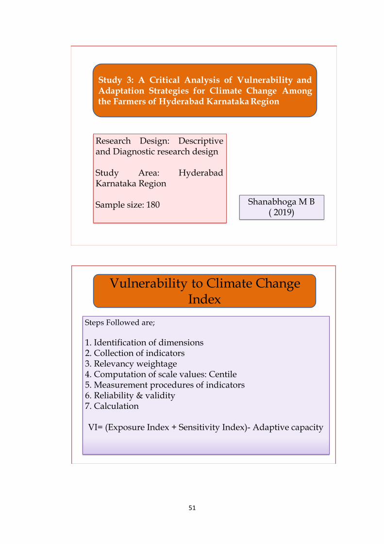
Study 3: A Critical Analysis of Vulnerability and Adaptation Strategies for Climate
Change Among the Farmers of Hyderabad Karnataka Region
Shanabhoga M B (2019)
Research Design: Descriptive and Diagnostic research design
Study Area: Hyderabad Karnataka Region
Sample size: 180
Steps Followed are:
1. Identification of dimensions
2. Collection of indicators

22
3. Relevancy weightage
4. Computation of scale values: Centile
5. Measurement procedures of indicators
6. Reliability & validity
7. Calculation
VI= (Exposure Index + Sensitivity Index)- Adaptive capacity
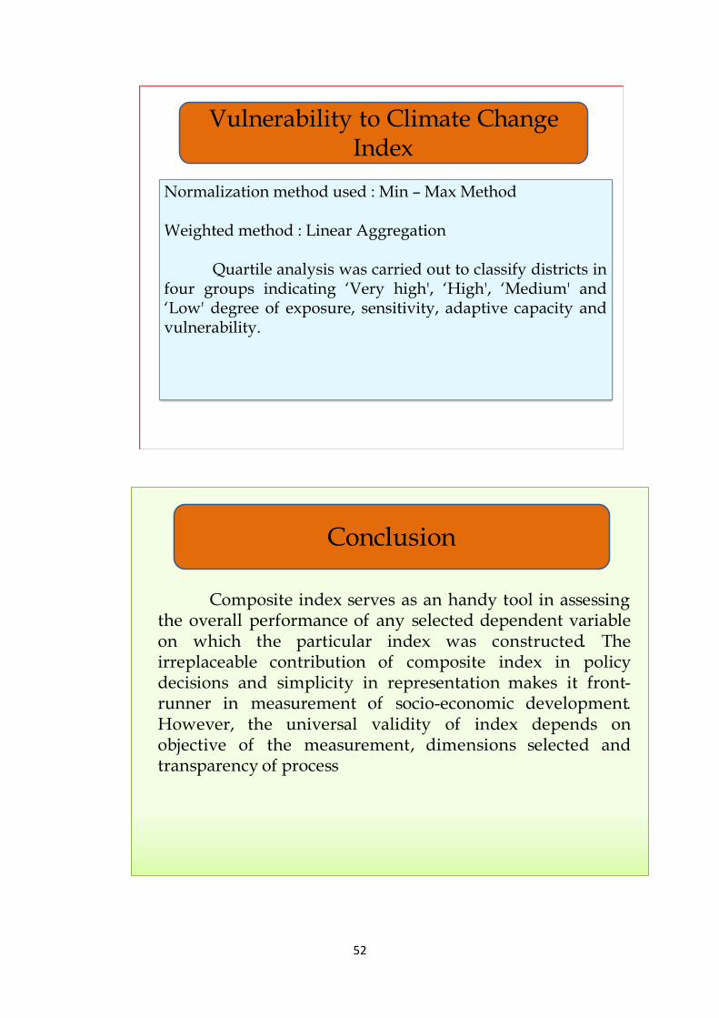
8. Summary
Composite index serves as a handy tool in assessing the overall performance of any
selected dependent variable on which the particular index was constructed. The irreplaceable
contribution of composite index in policy decisions and simplicity in representation makes it
front-runner in measurement of socio-economic development. However, the universal validity
of index depends on objective of the measurement, dimensions selected and transparency of
process.
9. Discussion
1. Min-Max weightage method uses decimal values?
Absolutely, the Min-Max method uses decimals in between 0 to 1.
2. What are the issues in constructing the composite index?
The data availability is main issue and also the judgement of appropriate combination
of weightage, aggregation and other steps should come with experience in the index
development. It also won’t bring sometimes the root cause of the problem where its
primary objective is to bring big picture.
3. Do indicators and variables same?
Variable term is very broader and that should be varied in results with in the population.
The indicators some times treated as variable when they are in measurable forms. The
index structure and the whole research structure we make during our research with
different variables where index construction is a part to measure a variable. These
structures should be seen differently.
4. What it is meant by outliers?
The extreme values of the data that disturb the normal data and its measurements. These
outliers are special cases which can’t be applied to the population. Thus, we try different
methods to solve these.
23
5. When to use different aggregation techniques?
Generally, the additive/linear model is mostly used. The geometric aggregation method
is little complex comparatively as we measure with different data at indicator (raw data)
and dimension levels (normalized data). Based on research data, time and other
parameters the techniques are selected.
6. What is difference between Scale and Index?
In scale the construct starts first and variables were reflected based on construct whereas
in the index the group of variables form the construct. This is the major difference
between the scale and index. It is so easy to explain but lot of conceptual and ground
level understanding is need to select between these options.
7. Whether Scale or Index which is better measurement technique?
Here judgement is so difficult when they serve different purpose. One strictly gives
overall information for policy decisions and the scale to get gross rot empirical evidence
with underlying factors of attitude and knowledge.
8. Why such complicated process for development when there are other simple
measurement techniques?
The complicated process like PCA output emphasizes the statistical validity of the
model developed which makes the results more acceptable than the simple analytical
methods. However, the best fitness method is more value than the more
complicated/available one.
9. What do you suggest for coming scholars to choose between index and scale?
As mentioned above direction of construct and variables is primary criteria. The
multidimensionality best embedded in the index than scale where many scale
development process includes uni-dimensionality.
References
BANDURA, R., 2008, A survey of composite indices measuring country performance: 2008
update. New York: United Nations Development Programme, Office of Development
Studies (UNDP/ODS Working Paper).
FAGERBERG, J., 2002, Europe at the crossroads: the challenge from innovation-based
growth. The globalizing learning economy, 45-60.
DARSANA, 2018, Development Programmes and their Impact on Farmers’ Welfare in Kerala.
Ph.D. Thesis (Unpub.), University of Agricultural Sciences, Bangalore.
Joint Research Centre-European Commission, 2008, Handbook on constructing composite
indicators: methodology and user guide. OECD publishing.
MAZZIOTTA, M., & PARETO, A., 2013, Methods for constructing composite indices: One
for all or all for one. Rivista Italiana di Economia Demografia e Statistica, 67(2), 67-
80.
24
PAUL, S., 2012, Work styles, best practices and productivity of agricultural scientists. Ph.D.
Thesis (Unpub.), Indian Agricultural Research Institute, New Delhi.
SMITH, V. H., 1998, Measuring the benefits of social science research (Vol. 2). Intl Food
Policy Res Inst.
VENKAIAH, K., MESHRAM, I. I., MANOHAR, G., RAMAKRISHA, K., & LAXMAIAH,
A., 2015, Development of composite index and ranking the districts using nutrition
survey data in Madhya Pradesh, India. Indian Journal of Community Health, 27(2),
204-210.
SHANABHOGA, M. B., KRISHNAMURTHY, B. AND VINAYKUMAR, R., 2019,
Development of a vulnerability index to assess vulnerability status of the farmers and
district due to climate change. International J. of Advanced Biological Res., 9(3): 238-
247.
IYENGAR, N. S., AND SUDARSHAN, P., 1982, A method of classifying regions from
multivariate data. Economic and political weekly, 2047-2052.
25
UNIVERSITY OF AGRICULTURAL SCIENCES, BANGALORE,
DEPARTMENT OF AGRICULTURAL EXTENSION,
COA, GKVK, BENGALURU-65
Name: GOPICHAND, B Date : 05-12-2020
ID No: PALB 8025 Time : 09:30 AM
Class : III Ph. D. Venue: Dwarakinath Hall
Seminar III Synopsis
Construction of Composite Index
The more valid Agricultural Extension research methodology includes the construction
of scale and composite index. The scale development is most common measurement
technique used by researchers and scholars of different social science domains. The other
kind of measurement composite index is collection of large number of indicators or variables
that aggregate to measure overall performance. It is increasingly recognised tool for policy
decisions. It became a means to start a discussion which ideally measures the
multidimensional concepts. The Google scholar search result from 2016 to 1st Dec., 2020 gives
7,92,000 publications related to composite index depicts, how widely it is being used. The
robust, discriminating, efficient and effectiveness are the characteristics of an index. With
this background, the present seminar has been conceptualized with the following objectives:
4. To know the concept of composite index
5. To understand different normalization, weighted and aggregation methods in
composite index construction
6. To review the related research studies
The comprehensive index development process includes 10 steps. Choices made in
each step have important implications for others. Therefore, the composite indicator builder
has not only to make the appropriate methodological choices but also to identify whether
they fit or not. The initial step, theoretical framework will be constructed by establishing
linkage between variables, indicators and dimensions. Therefore, understanding the multi-
dimensional phenomenon is very crucial at this step. The data selection and missing data
steps are to be operationalized before the normalization of data. This is very important to
bring common scaling to indicators. The methods include the ranking the simplest technique,
standardization makes each indicator mean, 0 and S.D., 1. The Min-Max method normalize
the indicators within the range 0 to 1, which uses different formulae for positive and negative
implications to fall in predetermined range. Further, distance from reference point method,
the benchmark established based on certain criteria and comparison with the bench mark
gives normalized values. The other methods were categorical scale based on points given to
different percentile ranges and indicators above and below mean -1 to +1 without any further
differentiation in scores.
26
After the normalization, each indicator should be weighted by addition of each unit to
the indicator. Most composite indicators rely on equal weightage which lack statistical
ground. The Principal Component Analysis groups the indicators based on the collinearity
statistically. However, it needs very high sample size. Data envelopment model measures the
distance between countries. In unobserved component analysis, shedding light on some
unknown component will give the weightage. Analytical hierarchy process considers expert
opinion on different indicators in the model of paired comparison technique. The weightage
is followed by aggregation of weights which include the additive, geometric and multi-criteria
approaches. Compensability is poor performance of one indicator is compensated by other
while aggregating. The additive model is completely compensatory whereas the multi criteria
is non-compensatory.
Research Studies
Paul (2012) developed the research productivity index by subjective weighting of
dimensions and indicators by experts. The relative weightage and scoring based on
achievement of scientist with dimensions scientific publication, product development,
research activities undertaken, teaching activities undertaken, extension activities
undertaken, awards received and recognition achieved.
Shanabhoga (2019) constructed the vulnerability to climate change index with Min-
max normalization technique with initial experts ranking dimensions and indicators suggested
by Guilford (1954). The dimensions were exposure, sensitivity and adaptive capacity with
scale values 5.17, 4.46 and 4.70 respectively.
Conclusion
The irreplaceable contribution of composite index in policy decisions and simplicity in
representation makes it front-runner in measurement of socio-economic development.
However, the universal validity of index depends on objective of the measurement and
transparency in the process employed.
References
PAUL, S., 2012, Work styles, best practices and productivity of agricultural scientists. Ph.D. Thesis (Unpub.), Indian Agricultural Research Institute, New Delhi.
SHANABHOGA, M. B., KRISHNAMURTHY, B. AND VINAYKUMAR, R., 2019, Development of a
vulnerability index to assess vulnerability status of the farmers and district due to climate change. International J. of Advanced Biological Res., 9(3): 238-247.

27
Presentation Slides

28

29
30

31

32
33
34

35
36
37
38
39
40
41
42
43

44
45
46
47
48
49
50
51
52

53
Recommended