Lecture Notes on Stochastic Processes
Frank Noé, Bettina Keller and Jan-Hendrik Prinz
July 17, 2013

1
[email protected], [email protected], [email protected]
DFG Research Center Matheon, FU Berlin, Arnimallee 6, 14195 Berlin, Ger-many
July 17, 2013
Contents
1 Introduction and Overview 5
1.1 Overview . . . . . . . . . . . . . . . . . . . . . . . . . . . . . . . . 5
1.2 Some terms from measure theory . . . . . . . . . . . . . . . . . . 5
1.3 Probabilities, probability spaces and discrete random variables . 8
1.4 Random Variables . . . . . . . . . . . . . . . . . . . . . . . . . . 9
1.5 Central Limit Theorem . . . . . . . . . . . . . . . . . . . . . . . . 12
2 Markov chains 14
2.1 General Properties of space-discrete Markov processes . . . . . 16
2.2 Time-Discrete Markov Chains . . . . . . . . . . . . . . . . . . . 18
2.3 Markov chain Monte Carlo (MCMC) . . . . . . . . . . . . . . . . 25
3 Analysis of Markov Chains 30
3.1 Hitting and Splitting/Committor Probabilities . . . . . . . . . . 30
3.2 Transition path theory / Reactive Flux: . . . . . . . . . . . . . . . 33
3.3 Eigenvector decomposition and interpretation . . . . . . . . . . 36
3.4 Timescales and timescale test . . . . . . . . . . . . . . . . . . . . 39
3.5 Correlation functions . . . . . . . . . . . . . . . . . . . . . . . . . 40
4 Continuous Random variables 43
4.1 Continuous random variables . . . . . . . . . . . . . . . . . . . . 44
4.2 Properties of Random Variables X ∈ R . . . . . . . . . . . . . . . 45
4.3 Transformation between random variables . . . . . . . . . . . . 46
4.4 Linear Error Propagation . . . . . . . . . . . . . . . . . . . . . . . 48
4.5 Characteristic Functions . . . . . . . . . . . . . . . . . . . . . . . 52
2
CONTENTS 3
5 Markov chain estimation 54
5.1 Bayesian Approach . . . . . . . . . . . . . . . . . . . . . . . . . . 54
5.2 Transition Matrix Estimation from Observations; Likelihood . . 55
5.3 Maximum Probability Estimator . . . . . . . . . . . . . . . . . . 57
5.4 Maximum Likelihood Estimator of Reversible Matrices . . . . . 58
5.5 Error Propagation . . . . . . . . . . . . . . . . . . . . . . . . . . . 59
5.6 Full Bayesian Estimation . . . . . . . . . . . . . . . . . . . . . . . 62
5.6.1 Metropolis-Hastings sampling . . . . . . . . . . . . . . . 63
5.6.2 Non-reversible shift element . . . . . . . . . . . . . . . . 64
5.6.3 Reversible shift element . . . . . . . . . . . . . . . . . . . 64
5.6.4 Row Shift . . . . . . . . . . . . . . . . . . . . . . . . . . . 66
6 Markov Jump Processes 69
6.1 Poisson process . . . . . . . . . . . . . . . . . . . . . . . . . . . . 70
6.2 Markov Jump Process . . . . . . . . . . . . . . . . . . . . . . . . 72
6.3 Master equation . . . . . . . . . . . . . . . . . . . . . . . . . . . . 74
6.4 Solving very large systems . . . . . . . . . . . . . . . . . . . . . . 77
6.5 Hitting Probabilities, Committors and TPT fluxes . . . . . . . . 79
7 Continuous Markov Processes 81
7.1 Random Walk . . . . . . . . . . . . . . . . . . . . . . . . . . . . . 81
7.1.1 Long-time approximation and transition to continuousvariables . . . . . . . . . . . . . . . . . . . . . . . . . . . . 81
7.1.2 Wiener Process and Brownian dynamics . . . . . . . . . 83
7.2 Langevin and Brownian Dynamics . . . . . . . . . . . . . . . . . 84
7.2.1 Applications . . . . . . . . . . . . . . . . . . . . . . . . . . 85
7.2.2 Further reading . . . . . . . . . . . . . . . . . . . . . . . . 86
8 Markov model discretization error 87
8.1 Basics . . . . . . . . . . . . . . . . . . . . . . . . . . . . . . . . . . 87
8.2 Spectral decomposition . . . . . . . . . . . . . . . . . . . . . . . . 88
8.3 Raleigh variational principle . . . . . . . . . . . . . . . . . . . . . 89
8.4 Ritz method . . . . . . . . . . . . . . . . . . . . . . . . . . . . . . 92
8.5 Roothaan-Hall method . . . . . . . . . . . . . . . . . . . . . . . . 93
8.6 Results . . . . . . . . . . . . . . . . . . . . . . . . . . . . . . . . . 95
CONTENTS 4
9 Stochastic vs. Transport Equations 98
9.1 Stochastic Differential Equations (SDE) . . . . . . . . . . . . . . 98
9.1.1 Terminology . . . . . . . . . . . . . . . . . . . . . . . . . . 98
9.1.2 Stochastic Processes . . . . . . . . . . . . . . . . . . . . . 99
9.1.3 Further Reading . . . . . . . . . . . . . . . . . . . . . . . 100
9.2 Master-Equation to Fokker-Planck . . . . . . . . . . . . . . . . . 100
9.3 Stochastic Integrals . . . . . . . . . . . . . . . . . . . . . . . . . . 102
9.3.1 Ito-Integral . . . . . . . . . . . . . . . . . . . . . . . . . . 103
9.3.2 Stratonovich Integral . . . . . . . . . . . . . . . . . . . . . 105
10 Discretization 106
Chapter 1
Introduction and Overview
1.1 Overview
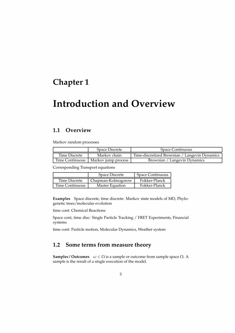
Markov random processes
Space Discrete Space Continuous
Time Discrete Markov chain Time-discretized Brownian / Langevin DynamicsTime Continuous Markov jump process Brownian / Langevin Dynamics
Corresponding Transport equations
Space Discrete Space Continuous
Time Discrete Chapman-Kolmogorow Fokker-PlanckTime Continuous Master Equation Fokker-Planck
Examples Space discrete, time discrete: Markov state models of MD, Phylo-genetic trees/molecular evolution
time cont: Chemical Reactions
Space cont, time disc: Single Particle Tracking / FRET Experiments, Financialsystems
time cont: Particle motion, Molecular Dynamics, Weather system
1.2 Some terms from measure theory
Samples / Outcomes ω ∈ Ω is a sample or outcome from sample space Ω. Asample is the result of a single execution of the model.
5
CHAPTER 1. INTRODUCTION AND OVERVIEW 6
Examples:
Coin toss: Ω = heads, tailsDie roll: Ω = 1, 2, 3, 4, 5, 6Roulette: Ω = 0, ..., 36Gaussian random variable: Ω = R.
Events An event E is a set containing zero or more outcomes. Events are de-fined because in many situations individual outcomes are of little practical use.More complex events are defined in order to characterize groups of outcomes.
Examples:
Die roll: even = 2, 4, 6, odd = 1, 3, 5Events may be non-exclusive, e.g.
Roulette: red = 1, 3, 5, ..., black = 2, 4, 6, ..., 0 = 0, even, odd, ...
All intervals on the real axis: ix1,x2 = [x1, x2] | x1 ≤ x2; x1, x2 ∈ R
Algebra In stochastics, the term algebra is used to refer to the event set above,and it is a collection of sets of samples ω with particular properties. It is notrelated to the term algebra as a field of mathematics.
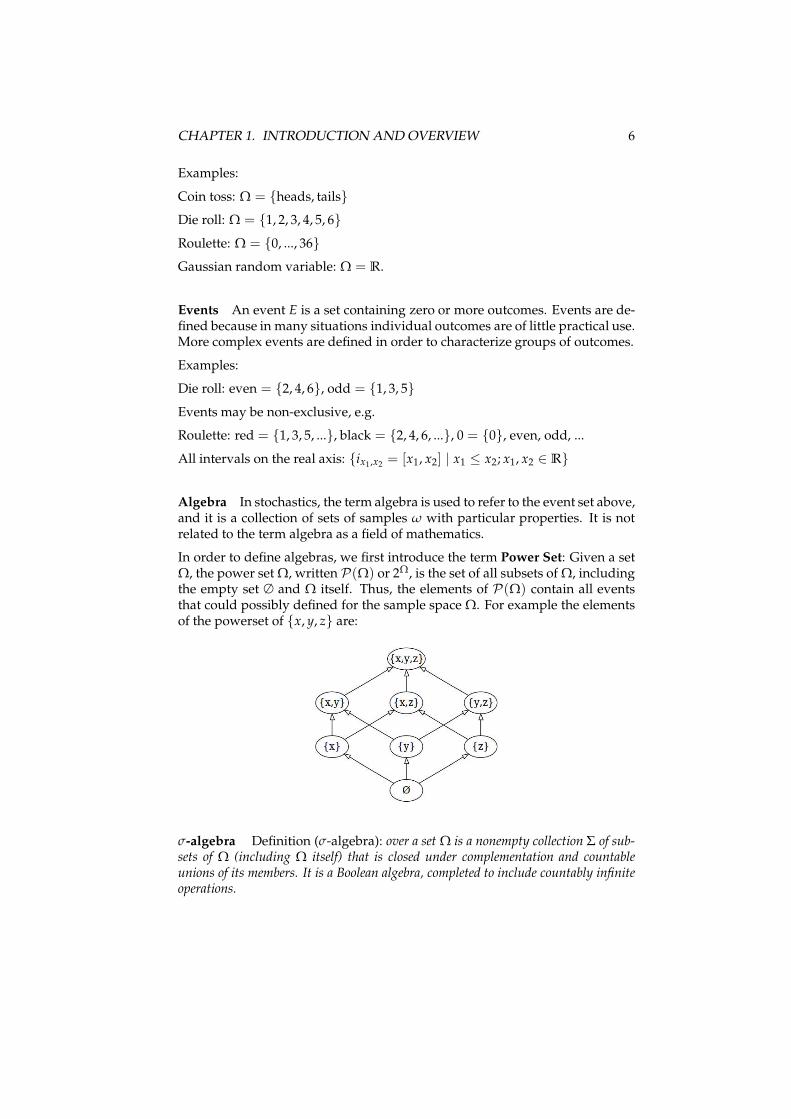
In order to define algebras, we first introduce the term Power Set: Given a setΩ, the power set Ω, written P(Ω) or 2Ω, is the set of all subsets of Ω, includingthe empty set ∅ and Ω itself. Thus, the elements of P(Ω) contain all eventsthat could possibly defined for the sample space Ω. For example the elementsof the powerset of x, y, z are:
σ-algebra Definition (σ-algebra): over a set Ω is a nonempty collection Σ of sub-sets of Ω (including Ω itself) that is closed under complementation and countableunions of its members. It is a Boolean algebra, completed to include countably infiniteoperations.
CHAPTER 1. INTRODUCTION AND OVERVIEW 7
Example: if Ω = a, b, c, d, one possible σ algebra on Ω is:
Σ = ∅, a, b, c, d, a, b, c, d.
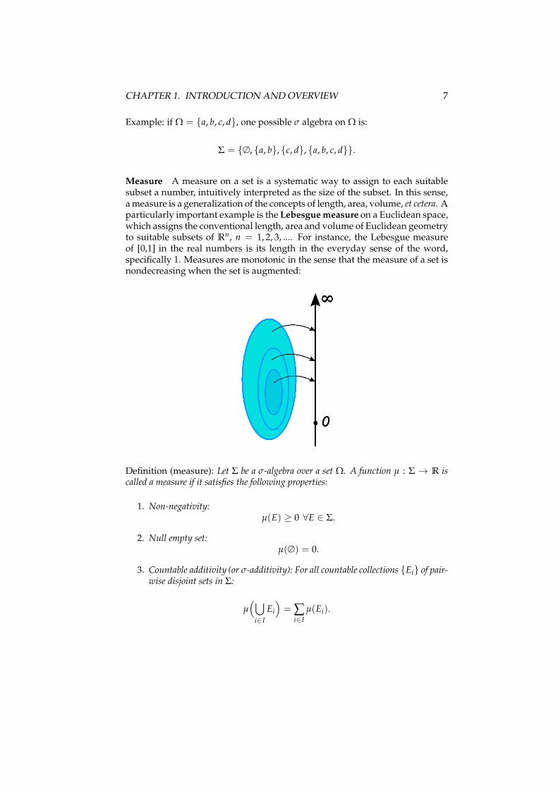
Measure A measure on a set is a systematic way to assign to each suitablesubset a number, intuitively interpreted as the size of the subset. In this sense,a measure is a generalization of the concepts of length, area, volume, et cetera. Aparticularly important example is the Lebesgue measure on a Euclidean space,which assigns the conventional length, area and volume of Euclidean geometryto suitable subsets of R
n, n = 1, 2, 3, .... For instance, the Lebesgue measureof [0,1] in the real numbers is its length in the everyday sense of the word,specifically 1. Measures are monotonic in the sense that the measure of a set isnondecreasing when the set is augmented:
Definition (measure): Let Σ be a σ-algebra over a set Ω. A function µ : Σ → R iscalled a measure if it satisfies the following properties:
1. Non-negativity:µ(E) ≥ 0 ∀E ∈ Σ.
2. Null empty set:µ(∅) = 0.
3. Countable additivity (or σ-additivity): For all countable collections Ei of pair-wise disjoint sets in Σ:
µ(⋃
i∈I
Ei
)
= ∑i∈I
µ(Ei).
CHAPTER 1. INTRODUCTION AND OVERVIEW 8
Measure space Definition (measure space): is a triple (Ω, Σ, µ) containing anonempty set Ω a σ-Algebra Σ on Ω and a measure µ : Σ → R
1.3 Probabilities, probability spaces and discrete ran-
dom variables
Probability measure Definition (probability measure): P is a measure with theadditional property that µ(Σ) = 1.
This can be ensured by normalizing another measure:
P(E) =µ(E)
µ(Σ).
We call P(E) the probability of E. As a consequence, the measure of the com-plement is:
P(EC) = 1 − P(E). ∀E ∈ Σ
In the case that all samples are equally likely, the probability of a particularevent E is given by the ratio of the number of combinations leading to E overthe total number of combinations:
P(E) =nE
ntot
For example consider drawing black or white balls from a large urn given thatfor each draw the probability of black or white is equal. We are interested in theprobability of getting k black balls in n ≥ k draws, where we are not interestedin the sequence of the draw. The number of ways to draw k black balls is givenby the binomial coefficient:
(n
k
)
=n!
k! (n − k)!=
n · (n − 1) · · · (n − k + 1)
k · (k − 1) · · · 1if k ∈ 0, 1, . . . , n,
The total number of combinations is 2n, and thus the probability is
P(k) = 2−n
(n
k
)
CHAPTER 1. INTRODUCTION AND OVERVIEW 9
Conditional Probability Definition (conditional probability): The conditionalprobability of event A given B is given by
P(A | B) =P(A ∩ B)
P(B), (whence P(B) 6=0)
Here A ∩ B is the intersection of A and B, that is, it is the event that both eventsA and B occur.
Independence Definition (independence): Two events A and B are independentif and only if
P(A ∩ B) = P(A)P(B)
More generally, any collection of events-possibly more than just two of them-are mu-tually independent if and only if for any finite subset A1, ..., An of the collection wehave
P
(n⋂
i=1
Ai
)
=n
∏i=1
P(Ai).
This is called the multiplication rule for independent events.
Probability space Definition (probability space): is a measure space (Ω, Σ, P)with a probability measure P. Ω is called sample space and E ∈ Σ are the events. EC
is called counter event. P(E) is called probability and P(EC) counter probability of E.
Once the probability space is established, it is assumed that “nature” makes itsmove and selects a single outcome, ω, from the sample space Ω. Then we saythat all events from F containing the selected outcome ω (recall that each eventis a subset of Ω) “have occurred”. The selection performed by nature is donein such a way that if we were to repeat the experiment an infinite number oftimes, the relative frequencies of occurrence of each of the events would havecoincided with the probabilities prescribed by the function P.
1.4 Random Variables
Given a probabilty space (Ω, Σ, P), a discrete random variable X(ω) : Ω → R
is a map from outcomes to values. We will first take a look at discrete randomvariables
Example 1: Coin toss. State space Ω = heads, tails. We can introduce arandom variable Y as follows:
CHAPTER 1. INTRODUCTION AND OVERVIEW 10
Y(ω) =
1, if ω = heads,
0, if ω = tails.
Example 2: Die roll. State space Ω = 1, 2, 3, 4, 5, 6. The “even” function e(ω)is given by
e(ω) =
0, if one of 1,3,5 is rolled,
1, if one of 2,4,6 is rolled,
Probability density function In probability theory, a probability density func-tion (abbreviated as pdf, or just density) of a continuous random variable is afunction that describes the relative likelihood for this random variable to occurat a given point in the observation space. The probability of a random variablefalling within a given set is given by the integral of its density over the set.
A probability density function is most commonly associated with continuousunivariate distributions. In the discrete case, the probability density
fX(x) = P[x]
is identical with the probability of an outcome, and is also called probabilitydistribution.
Example 1: coin toss
fY(y) =
12 , if y = 1,12 , if y = 0.
Example 2: die roll
fX(x) =
16 , if x = 1, 2, 3, 4, 5, 6,
0, otherwise.
We have that probability density can be summed over sets:
P[A] = ∑x∈A
P[x] = ∑x∈A
fX(x)
and the cumulative density function is given by:
FX(x0) = P[x ≤ x0] = ∑x≤x0
P[x] = ∑x≤x0
fX[x]
CHAPTER 1. INTRODUCTION AND OVERVIEW 11
As a result of normalization:
FX(−∞) = 0
FX(∞) = 1
Moments: expectation, variance, covariance If f is a probability density func-tion, then the value of the following integral above is called the nth moment ofthe probability distribution.
µn = E(xn) = ∑x∈Ω
xn f (x)
The first moment is the mean (µ1 or in short µ). For any two random variablesX, Y it holds that
µ1(X + Y) = E(X +Y) = ∑x∈Ω
∑y∈Ω
x f (x) + y g(y) = E(X) + E(Y)
The nth central moment of the probability distribution of a random variable Xis
µn = E((X − µ)n).
For example:
µ2 = Var(x) = E((x − µ)2)
= E(x2 − 2xµ + µ2) = E(x2)− 2µE(x) + µ2
= E(x2)− µ2
For the variance of X + Y we have the integral
Var(X + Y) = E((x − µx) + (y − µy))2)
= E((x − µx)2) + 2E((x − µx)(y − µy)) + E((y − µy))
2)
= Var(X) + 2Cov(X, Y) + Var(Y)
CHAPTER 1. INTRODUCTION AND OVERVIEW 12
Correlation or Pearson’s correlation coefficient is defined by:
Corr(X, Y) =Cov(X, Y)
√
Var(X)Var(Y)
For uncorrelated random variables it holds that:
Var(X +Y) = Var(X) + Var(Y)
as then Cov(X, Y) = 0. Note that correlation does not imply independence.
Independence Definition (independent random variables): Two random vari-ables X and Y are independent if and only if for any numbers a and b the eventsX ≤ a and Y ≤ b are independent events as defined above. Similarly an arbitrarycollection of random variables – possible more than just two of them—is independentprecisely if for any finite collection X1, ..., Xn and any finite set of numbers a1, ..., an,the events X1 ≤ a1, ..., Xn ≤ an are independent events as defined above.
For independent random variables it holds for any moments:
µn(X +Y) = µn(X) + µn(Y)
If two variables are independent, then they are also uncorrelated. The converseof these, i.e. the proposition that if two random variables have a correlation of0 they must be independent, is not true.
Furthermore, random variables X and Y with probability densities fX(x) andfY(y), are independent if and only if the combined random variable (X, Y) hasa joint distribution
fX,Y(x, y) = fX(x) fY(y)
1.5 Central Limit Theorem
The central limit theorem states that when a random effect results from the sumof many independent random variables, each of them having a finite varianceboth otherwise from arbitrary distributions, then this summed effect will tends
CHAPTER 1. INTRODUCTION AND OVERVIEW 13
towards a Gaussian distribution. This is the reason why Gaussian distributionsare so ubiquitously found: Many real-life processes are complex in the sensethat they result from the interaction of many stochastic degrees of freedom,thus the central limit theorem kicks in and produces Gaussian distributions ofobserved variables.
The proof of the CLT will come later in the continuous random variable sec-tion. For now, we’ll just give the following statements: Let Sn be the sum of nindependent random variables with zero mean and variance σ2, given by
Sn = X1 + · · ·+ Xn.
Then, if we define new random variables
Zn =Sn − nµ√
n=
Sn√n=
n
∑i=1
Xi√n
,
thenlim
n→∞P(Zn) = N (0, σ2) :
they will converge in distribution to the normal distribution N (0, σ2) as n ap-proaches infinity. N (0, σ2) is thus the asymptotic distribution of Zn. Zn canalso be expressed as
Zn =√
n(Xn − µ) =√
n Xn,
where
Xn =Sn
n=
1
n(X1 + · · ·+ Xn)
is the sample mean. It directly follows that the quantity Zn/√
n = (Xn − µ) =Xn, i.e. the estimation error of the mean, has a variance of σ2/n. For anyrandom variable X:
VarXn − E(X) =Var(X)
n
for n independent samples.
Chapter 2
Markov chains
We will now focus our attention to Markov chains and come back to space-continuous processes later. The motivation for this is that whenever studyinga space-continuous process in practice, it needs to be in some way discretized,and thus effectively becomes a Markov chain. The numerical properties of sucha discretization will be studied later.
Let X = 1, ..., n be a discrete state space and let x(t) be a Markov chain (withthe Markov property as defined above) on X, where t may be either discrete orcontinuous. The system “jumps” between the states of X in time. Such a jumpis called a transition.
Time-discrete Markov processes All of the processes we had described hereare Markov processes they are defined by the fact that the propagation of thesystem is entirely determined by knowing its present state xt, and is thus inde-pendent on its past. Formally, for discrete times:
P(x(t) | x(t − 1), x(t − 2), ..., x(1)) = P(x(t) | x(t − 1))
The dynamics then is entirely defined by the transition probabilities P(x(t) |x(t − 1)) : [X × X] → R . In the state-continuous case this is a transitiondensity that acts between points of the state space. In the state-discrete casethis is a transition (probability) matrix, often denoted by P = [Pij] or T = [Tij].
Higher-order Markov chains A Markov chain of order m (or a Markov chainwith memory m) where m is finite, is a process satisfying
P(x(t) | x(t− 1), x(t− 2), ..., x(1)) = P(x(t) | x(t− 1), x(t− 2), ..., x(t−m)) for t > m
14
CHAPTER 2. MARKOV CHAINS 15
In other words, the future state depends on the past m states. It is possible toconstruct a chain (y(t)) from (x(t)) which has the ’classical’ Markov propertyas follows:
Let y(t) = (x(t), x(t − 1), ..., y(t − m + 1)), the ordered m-tuple of x values.Then y(t) is a Markov chain with state space Xm and has the classical Markovproperty. This is a result of Taken’s embedding theorem.
Applications (see Wiki pages)
Internet applications The PageRank of a webpage as used by Google is de-fined by a Markov chain. It is the probability to be at page i in the stationarydistribution on the following Markov chain on all (known) webpages. If N isthe number of known webpages, and a page i has ki links then it has transition
probability αki+ 1−α
N for all pages that are linked to and 1−αN for all pages that
are not linked to. The parameter α is taken to be about 0.85.
Markov models have also been used to analyze web navigation behavior ofusers. A user’s web link transition on a particular website can be modeled us-ing first- or second-order Markov models and can be used to make predictionsregarding future navigation and to personalize the web page for an individualuser.
Economics and finance Markov chains are used in Finance and Economicsto model a variety of different phenomena, including asset prices and mar-ket crashes. The first financial model to use a Markov chain was the regime-switching model of James D. Hamilton (1989), in which a Markov chain is usedto model switches between periods of high volatility and low volatility of as-set returns. A more recent example is the Markov Switching Multifractal assetpricing model, which builds upon the convenience of earlier regime-switchingmodels It uses an arbitrarily large Markov chain to drive the level of volatilityof asset returns.
Dynamic macroeconomics heavily uses Markov chains. An example is usingMarkov chains to exogenously model prices of equity (stock) in a general equi-librium setting.
Mathematical biology Markov chains also have many applications in bio-logical modelling, particularly population processes, which are useful in mod-elling processes that are (at least) analogous to biological populations. TheLeslie matrix is one such example, though some of its entries are not proba-bilities (they may be greater than 1). Another important example is the mod-eling of cell shape in dividing sheets of epithelial cells. The distribution ofshapes—predominantly hexagonal—was a long standing mystery until it wasexplained by a simple Markov Model, where a cell’s state is its number of sides.
CHAPTER 2. MARKOV CHAINS 16
Empirical evidence from frogs, fruit flies, and hydra further suggests that thestationary distribution of cell shape is exhibited by almost all multicellular an-imals. Yet another example is the state of Ion channels in cell membranes.
Gambling Markov chains can be used to model many games of chance. PersiDiakonis, a famous mathematician currently in Stanford, has proven severaltheorems concerning the decorrelation of Markov chains. One such proof showsthat the number of times a deck of cards needs to be shuffled in order to be con-sidered to be well shuffled is 7.
2.1 General Properties of space-discrete Markov pro-
cesses
(also valid for Markov jump processes, see below)
Time-homogeneity Time-homogeneous Markov chains (or stationary Markovchains) are processes where
P(x(t + 1) = i|x(t) = j) = P(x(s + t + 1) = i|x(s + t) = j)
for all s. The probability of the transition is an invariant property of the system,i.e. independent of the time when we evaluate the Markov chain.
Reducibility A state j is said to be accessible from a state i (written i → j) ifa system started in state i has a non-zero probability of transitioning into statej at some point. Formally, state j is accessible from state i if there exists a timet ≥ 0 such that
P(x(t) = j|x(0) = i) > 0.
Allowing t to be zero means that every state is defined to be accessible fromitself.
A state i is said to communicate with state j (written i ↔ j) if both i → j andj → i. A set of states C is a communicating class if every pair of states in Ccommunicates with each other, and no state in C communicates with any statenot in C. A communicating class is closed if the probability of leaving the classis zero, namely that if i is in C but j is not, then j is not accessible from i.
Finally, a Markov chain is said to be irreducible if its state space is a singlecommunicating class; in other words, if it is possible to get to any state fromany state.
CHAPTER 2. MARKOV CHAINS 17
Recurrence A state i is said to be transient if, given that we start in state i,there is a non-zero probability that we will never return to i. Formally, let therandom variable Ti be the first return time to state i:
Ti = inft ≥ 1 : x(t) = i | x(0) = i.
Then, state i is transient if and only if:
P(Ti = ∞) > 0.
If a state i is not transient (it has finite hitting time with probability 1), then itis said to be recurrent or persistent. Although the hitting time is finite, it neednot have a finite expectation. Let Mi be the expected return time,
Mi = E[Ti].
Then, state i is positive recurrent if Mi is finite; otherwise, state i is null re-current (the terms non-null persistent and null persistent are also used, respec-tively).
A state i is called absorbing if it is impossible to leave this state.
Steady-state analysis and limiting distributions A Markov process has aunique stationary distribution π if and only if it is irreducible and all of itsstates are positive recurrent. Note that this in particular includes ergodic pro-cesses, because ergodicity is a stronger requirement. In that case, π is relatedto the expected return time:
πi =1
Mi.
Further, if the chain is both irreducible and aperiodic, then for any i and j,
limt→∞
P(x(t) = j | x(0) = i) =1
Mj.
Note that there is no assumption on the starting distribution; the chain con-verges to the stationary distribution regardless of where it begins. Such π iscalled the equilibrium distribution of the chain.
If a chain has more than one closed communicating class, its stationary dis-tributions will not be unique (consider any closed communicating class in thechain; each one will have its own unique stationary distribution. Any of thesewill extend to a stationary distribution for the overall chain, where the proba-bility outside the class is set to zero).
CHAPTER 2. MARKOV CHAINS 18
2.2 Time-Discrete Markov Chains
A Markov chain on X, named after Andrey Markov, is a discrete random pro-cess with the Markov property. A discrete random process means a systemwhich can be in various states, and which changes randomly in discrete steps.It can be helpful to think of the system as evolving once a minute, althoughstrictly speaking the "step" may have nothing to do with time. The Markovproperty states that the probability distribution for the system at the next step(and in fact at all future steps) only depends on the current state of the system,and not additionally on the state of the system at previous steps. Since the sys-tem changes randomly, it is generally impossible to predict the exact state ofthe system in the future. However, the statistical properties of the system at agreat many steps in the future can often be described. In many applications itis these statistical properties that are important.
An example of a Markov chain is a random walk on the number line whichstarts at zero and transitions +1 or −1 with equal probability at each step. Theposition reached in the next transitions only depends on the present positionand not on the way this present position is reached.
Transition Matrix We define the propagator / transition matrix P ∈ Rn×n
which describes the evolution of the chain:
pij ≥ 0 ∀i, j
∑j=1...n
pij = 1 ∀i
These conditions define a stochastic matrix. pij represents the transition proba-bility of state i to state j within one step of the system (which may correspondto a fixed physical time step τ):
pij = P[x(t + 1) = j | x(t) = i]
Markov chain (definition) We are given a countable set X = 1, ..., n calledstate space, a stochastic matrix P ∈ R
n×n, and a distribution p(0) ∈ Rn. The
series of random variables x(t), t = 0, 1, ..., T is called Markov chain of lengthT with initial distribution p(0) and transition matrix P if:
• x(0) has distribution p(0)
• x(t + 1) has distribution px(t), i.e. the x(t)-th row of P for all t ≥ 0.
CHAPTER 2. MARKOV CHAINS 19
That is, the next value of the chain depends only on the current value, not anyprevious values. Thus it is often said that “Markov chains have no memory”.Note that this is not exactly correct: Markov chains have memory depth 1.A process without memory would be given by a sequence of independentlydrawn random variables
Evolution P can be used to generate trajectories according to the definitionabove:
1. Draw x(1) from the initial distribution p0
2. Draw x(t + 1) from the discrete distribution [px(t),1, ..., px(t),n]
Alternatively, we can also consider the probability to be in a given state i attime t, pi(t). This can be viewed as the fraction of particles in each state. Theentire distribution of the system is described by the vector pt ∈ R
n. Thus thetime evolution can be described by the set of equations:
pj(t + 1) = ∑i
pij pi(t) ∀j
which is equivalently written by the matrix equation
p(t + 1)T = p(t)TP
Chapman-Kolmogorow Equation We use the transition matrix twice and ob-tain:
pj(t + 2) = ∑i
pij pi(t + 1)
= ∑i
∑k
pki pijpk(t + 1)
or
p(t + 2)T = p(t)TP2
Note that this is possible because of Markovianity. Think about the form ofpj(t + 2) if the transition probabilities would not only depend on the current,but also the previous state.
P can be used to transport this probability vector over longer times:
CHAPTER 2. MARKOV CHAINS 20
p(t)T = p(0)TPt.
The probability to go from i to j in t time steps is:
P(x(t) = j | x(0) = i) = [Pt]ij
Stationary Distribution A Markov process has a unique stationary distribu-tion π if and only if it is irreducible and all of its states are positive recurrent.The stationary distribution, by definition is the distribution that is unchangedby the action of P:
πT = πT P
we can also write this as
πT P = 1πT
PTπ = 1π
and see that this is an eigenvalue equation. Thus, π (and any multiple cπ,c ∈ R) is a left eigenvector of P with eigenvalue 1. Since an irreducible andpositively recurrent chain has a unique stationary distribution, for a chain theeigenvalue 1 is unique. For all other eigenvalues, it can be shown that theyhave a norm strictly smaller than 1.
We can also ask for the corresponding right eigenvalue and find that
P1 = 1
Proof:
P
1...1
=
∑j p1j1 = ∑j p1j
...
∑j pnj1 = ∑j pnj
=
1...1
.
CHAPTER 2. MARKOV CHAINS 21
Convergence towards the stationary distribution For any diagonalizable ma-trix P we can write:
Pri = riλi
P[
r1 · · · rn]
=[
r1 · · · rn]
λ1 0. . .
0 λn
PR = RΛ
P = RΛR−1
and likewise
liP = λili
l1...
ln
P =
λ1 0. . .
0 λn
l1...
ln
LP = ΛL
P = L−1ΛL
or
P = RΛL
We assume a chain that is irreducible and positively recurrent. We consider theChapman-Kolmogorow equation:
p(t)T = p(0)TPt
and diagonalize P:
p(t)T = p(0)T (RΛL)t
= p(0)TRΛtL
= p(0)Tn
∑i=1
λtiril
Ti
Since the chain is irreducible and positively recurrent, it will have a singleeigenvalue 1 and otherwise eigenvalues with norm <1. We order them as fol-lows:
CHAPTER 2. MARKOV CHAINS 22
λ1 = 1, λ2, ..., λn with |λk| ≤ |λk+1| for k > 1.
and can thus write:
p(t)T = p(0)Tλt1r1lT
1 + p(0)Tn
∑i=2
λtiril
Ti
= p(0)T1πT + p(0)Tn
∑i=2
λtiril
Ti
thus, the infinite time distribution is
pT∞ = lim
t→∞p(t)T
= p(0)T1πT + limt→∞
(
p(0)Tn
∑i=2
λtiril
Ti
)
but since |λi| < 1 for all i > 1, the terms on the right cancel and we see that theinfinite time distribution is indeed π:
pT∞ = p(0)T1πT
= p(0)T
π1 · · · πn...
...π1 · · · πn
=[
π1 ∑j pj(0) · · · πn ∑j pj(0)]
=[
π1 · · · πn]
= πT
Speed of convergence We are interested in how fast the stationary distribu-tion is reached. Consider the error
CHAPTER 2. MARKOV CHAINS 23
E(t) =∥∥∥πT − p(t)T
∥∥∥
=
∥∥∥∥∥
πT − πT − p(0)Tn
∑i=2
λtiril
Ti
∥∥∥∥∥
=
∥∥∥∥∥
p(0)Tn
∑i=2
λtiril
Ti
∥∥∥∥∥
=
∥∥∥∥∥
p(0)Tλt2r2lT
2 + p(0)Tn
∑i=3
λtiril
Ti
∥∥∥∥∥
Asymptotically, i.e. for times t ≫ −1/ ln |λ3|, all terms on the right will ap-proximately zero, and we obtain for this regime:
E(t) ≈ λt2
∥∥∥p(0)Tr2lT
2
∥∥∥
which means the error decays exponentially with λt2. When comparing to an
exponential decay function exp(−kt), The rate of this decay is k2 = − ln λ2 and
the timescale of this decay is t2 = k−12 = −1/ ln λ2.
Note that if the initial distribution already happens to be πT , we see that weget the coefficients:
∥∥πTril
Ti
∥∥ =
∥∥lT
1 rilTi
∥∥ for i > 1. However, as a result of the
diagonalization we have lTi rj = 〈li, rj〉 = 0 for all i 6= j, and thus all coefficients
become 0, showing that convergence is indeed immediate in this case.
Periodicity A state i has period k if any return to state i must occur in multi-ples of k time steps. Formally, the period of a state is defined as
k = gcdn : P(Xn = i|X0 = i) > 0
(where "gcd" is the greatest common divisor). Note that even though a statehas period k, it may not be possible to reach the state in k steps. For example,suppose it is possible to return to the state in 6, 8, 10, 12, ... time steps; then kwould be 2, even though 2 does not appear in this list.
If k = 1, then the state is said to be aperiodic i.e. returns to state i can occur atirregular times. Otherwise (k > 1), the state is said to be periodic with periodk.
It can be shown that every state in a communicating class must have overlap-ping periods with all equivalent-or-larger occurring sample(s).
CHAPTER 2. MARKOV CHAINS 24
Ergodicity A state i is said to be ergodic if it is aperiodic and positive recur-rent. If a Markov process is irreducible and all its states are ergodic, then theprocess is said to be ergodic.
It can be shown that a finite state irreducible Markov chain is ergodic if it hasan aperiodic state.
Reversible Markov chain / Detailed balance A Markov chain is said to bereversible if there is a π such that
πi pij = πj pji.
This condition is also known as the detailed balance condition.
Summing over i gives
∑i
πi pij = πj
so for reversible Markov chains, π is always a stationary distribution.
The idea of a reversible Markov chain comes from the ability to "invert" a con-ditional probability using Bayes’ Rule:
P(x(t) = i | x(t + 1) = j) =P(x(t) = i, x(t + 1) = j)
P(x(t + 1) = j)
=P(x(t) = i)P(x(t + 1) = j | x(t) = i)
P(x(t + 1) = j)
=πi
πjP(x(t + 1) = j | x(t) = i)
pji =πi
πjpij.
It now appears as if time has been reversed.
We can consequently define a backward propagator, which will be used later,as:
pij =πj
πipji
which is in the reversible case identical to the forward propagator ( pij = pij ∀i, j).
CHAPTER 2. MARKOV CHAINS 25
Further Reading:
1. J. Norris: “Markov Chains”. Cambride University Press.Parts available from: http://www.statslab.cam.ac.uk/~james/Markov/
2.3 Markov chain Monte Carlo (MCMC)
Monte Carlo idea The idea of Monte Carlo methods is to approximate a de-terministic quantity with a probabilistic method. While the idea is quite old,the first use of the term Monte Carlo can be traced back to von Neumann andUlam in the 1940s, who collaborated on the Manhattan project in Los Alamos.
For example, given that a circle inscribed in a square and the square itself havea ratio of areas that is π/4, the value of π can be approximated using a MonteCarlo method (see Wiki page on Monte Carlo):
1. Draw a square on the ground, then inscribe a circle within it.
2. Uniformly scatter N objects of uniform size (e.g. grains of rice) over thesquare.
3. Count the number of objects inside the circle, Nx.
4. The ratio Nx/N is an estimate of π/4. Multiply the result by 4 to estimateπ.
Monte Carlo methods are often useful in cases where integrals need to be com-puted and deterministic numerical approaches fail, e.g. because the domaincannot be explicitly written or the integration space is too high-dimensional.
Generally, if we draw N samples (x1, ..., xN) from a discrete domain X and ac-cept them according to probability distribution P(x), then we can approximatethe probability of a point x as
limN→∞
Nx
N= P(x)
which allows expectations to be calculated, e.g.
E(x) = ∑x∈Ω
xP(x) = limN→∞
1
N ∑i
xi
E(a(x)) = ∑x∈Ω
a(x)P(x) = limN→∞
1
N ∑i
a(xi)
or in the continuous case, where f (x) is the probability density:
CHAPTER 2. MARKOV CHAINS 26
E(x) =∫
x∈Ωdx x f (x) = lim
N→∞
1
N ∑i
xi
E(a(x)) =∫
x∈Ωdx a(x) f (x) = lim
N→∞
1
N ∑i
a(xi)
Metropolis Monte Carlo Metropolis Monte Carlo1 was the first MCMC al-gorithm proposed. MCMC algorithms use the Monte Carlo idea above butconstruct a Markov Chain of Monte Carlo moves that has an invariant distri-bution identical to the desired sample distribution P. The MCMC approachis useful for estimating probability density functions for which probability ra-tios P(x1)/P(x2) are easy to calculate, but integrals ∑x∈A P(x) are hard orimpossible to calculate analytically or with deterministic numerical methodsbecause the domain A is very complex or the integration space is very high-dimensional. Moreover, if there is only a small fraction of Ω where P(x) issignificantly greater than 0, then application of the direct Monte Carlo method(see circle example above) is not useful, as it leads to mostly low-probabilitysamples.
The Metropolis Monte Carlo algorithm is a special MCMC method designedfor physical or chemical systems that have an energy E(x) and where the sta-tionary distribution is given by the Boltzmann distribution
P(x) = Z−1 exp(−βE(x)) , (2.1)
x is the the state of the system, i.e. the conformation of a molecule, Z is thepartition function,
Z = ∑x∈Ω
exp(−βE(x))
with β = 1kBT where kB is the Boltzmann constant and T is the temperature.
We assume that we have a model that allows us to calculate E(x) and thus alsoexp(−βE(x)) for a given x, but we cannot calculate probabilities of large setsof states, especially Z, because we simply cannot afford to enumerate all states.Metropolis Monte Carlo defines a Markov chain with propagator P with thefollowing properties:
1. The chain is reversible, i.e. we have a stationary distribution π withπi pij = πj pji
2. The stationary distribution is exactly the distribution we want to samplefrom πi = P(i).
1Nicholas Metropolis, Arianna W. Rosenbluth, Marshall N. Rosenbluth, Augusta H. Teller, andEdward Teller, "Equation of State Calculations by Fast Computing Machines", Journal of ChemicalPhysics 21, 1087 (1953)
CHAPTER 2. MARKOV CHAINS 27
If we can construct a Markov chain we can generate realizations x(t) and esti-mate expectation values from it. For a given distribution P(x) there are manyways to construct a Markov chain which fulfills the above conditions and isthus able to generate estimates of P(x). They differ mainly by their computa-tional efficiency for different problems.
In the following we sketch the Metropolis Monte Carlo algorithm:
1. Pick a starting state x0
2. For k = 0 to N − 1:
(a) Pick a trial conformation xk → x′
(b) Calculate the probability ratio
P(x′)P(xk)
= exp(−β[E(x′)− E(xk)])
(c) Accept the trial move with probability
pacc = min1,P(x′)P(xk)
this can be realized by drawing a random number k ∈ [0, 1[ andaccepting if k ≤ pacc.
(d) If the trial move is accepted, xk+1 = x′, else xk+1 = xi
By looking at the acceptance criterion, we see that:
E(x′) > E(xi) ⇒ exp(−β∆E) < 1 ⇒ accepted if k < exp(−β∆E)E(x′) ≤ E(xi) ⇒ exp(−β∆E) ≥ 1 ⇒ accepted if k < 1, i.e. always
The algorithm is correct, i.e. it indeed generates a reversible Markov chainwith stationary distribution P(x), provided that following requirements arefulfilled:
1. The Boltzmann distribution can be evaluated at any point x.
2. The probability of making a trial move x → x′ is equal to the probabilityof making the reverse trial move, i.e. P(x → x′) = P(x′ → x)
3. Any point x′ can be reached from any other point x by making trialmoves, i.e. the Markov chain is irreducible.
CHAPTER 2. MARKOV CHAINS 28
Proof of Metropolis Monte Carlo
• Unique stationary distribution: Assumption 2 means that the constructedMarkov chain is positively recurrent, Assumption 3 means that it is irre-ducible. As a result, the constructed propagator P has a unique stationarydistribution.
• Reversibility: We call the probability to propose a move xi to xj is P(xi →xj) and vice versa P(xj → xi). The probability to move from xi to xj, i.e.to propose and accept, are pij and vice versa pji. Without restriction ofgenerality we assume E(xi) < E(xj). We find that:
pij = P(xi → xj) exp(−β[E(xj)− E(xi)]) = P(xi → xj)exp(−βE(xj))
exp(−βE(xi))= P(xi → xj)
P(xj)
P(xi)
pji = P(xj → xi)
by construction,
P(xi → xj) = P(xj → xi)
pijP(xi)
P(xj)= pji
resulting in the equations:
P(xi)pij = P(xj)pji ∀i, j
• It follows that P is a reversible chain with respect to the unique stationarydistribution π = P(x).
Metropolis-Hastings algorithm The Metropolis-Hastings algorithm is a gen-eralization of the above idea by Hastings 2. Let us not assume that the proposalprobabilites are symmetric, i.e. in general P(xi → xj) = P(xj → xi) is not truefor all i, j. Let us consider two points xi, xj with P(xi) ≥ P(xj) and accept
xi → xj with probabilityP(x j)P(x j→xi)
P(xi)P(xi→x j)and the reverse move with probability 1.
We reconsider the proof of the Metropolis Monte Carlo algorithm:
pij = P(xi → xj)P(xj)P(xj → xi)
P(xi)P(xi → xj)=
P(xj)P(xj → xi)
P(xi)
pji = P(xj → xi)
2Hastings, W.K., "Monte Carlo Sampling Methods Using Markov Chains and Their Applica-tions", Biometrika 57, pp. 97-109 (1970).
CHAPTER 2. MARKOV CHAINS 29
such that again:pijP(xi) = pjiP(xj).
This provides the following algorithm:
1. Pick a starting state x0
2. For k = 0 to N − 1:
(a) Propose a trial conformation xk → x′ with probability P(xi → x′)
(b) Accept the trial move with probability
pacc = min1,P(x′)P(x′ → xi)
P(xi)P(xi → x′)
(c) If the trial move is accepted, xk+1 = x′, else xk+1 = xi
Additionally to the requirements of the Metropolis Monte Carlo method weneed to be able the proposal probabilities P(xi → x′).
Remarks on the processes and convergences Consider the Markov processx(t) with stationary probability π and let us assume that we can simulate itsdynamics with the propagator Px. Along the previous analysis, the direct sim-ulation of this process will converge to π asymptotically with rate kx = − ln λx,where λx is the largest eigenvalue of Px that is smaller than 1.
We can construct a MCMC method which samples π via a different propa-gator Py. This MCMC process will converge to π asymptotically with rateky = − ln λy, where λy is the largest eigenvalue of Py that is smaller than 1.
Thus, it is important to distinguish the the original process and the MCMC pro-cess constructed to sample the stationary distribution of the original process.We can construct different processes that sample the same stationary distribu-tion. Clearly, depending on λy these processes can have very different efficien-cies. Ideally we would chose a strategy with λy < λx and thus obtain a fasterconvergence than the original process itself.
Chapter 3
Analysis of Markov Chains
3.1 Hitting and Splitting/Committor Probabilities
Hitting probabilites for Markov Chains Given a stochastic process on statespace X = 1, ...., n, the hitting time of set A: HA : X → 0, 1, 2, ... ∪ ∞ isdefined as:
HAi = inft ≥ 0 : x(t) ∈ A|x(0) = i
and the hitting probability is the probability that starting from i we ever hit A:
hAi = P(HA
i < ∞).
For a Markov chain on X with transition matrix P, the vector of hitting proba-bilities hA = (hA
i : i ∈ I) is the minimal non-negative solution to the system oflinear equations:
hAi = 1for i ∈ A
hAi = ∑
j∈X
pijhAj for i /∈ A.
(Minimality means that if x = (xi : i ∈ X) is another solution with xi ≥ 0 forall i, then xi ≥ hi for all i.)
Proof:
First we show that hA satisfies the above equation.
1) If x(0) = i ∈ A, then HAi = 0, so hA
i = 1.
30
CHAPTER 3. ANALYSIS OF MARKOV CHAINS 31
2) If x(0) = i /∈ A, then HAi ≥ 1, so by the Markov property:
P(HAi < ∞ | x(1) = j) = P(HA
j < ∞) = hAj
and
hAi = P(HA
i < ∞)
= ∑j∈X
P(HAi < ∞, x(1) = j)
= ∑j∈X
P(HAi < ∞ | x(1) = j)P(x(1) = j | x(0) = i)
= ∑j∈X
hAj pij.
Next, we show that hA are the minimal solution
1) Suppose that x = (xi : i ∈ I) is any solution to the equation. then hAi = xi =
1 for i ∈ A.
2) Suppose i /∈ A, then:
xi = ∑j∈X
pijxj = ∑j∈A
pij + ∑j/∈A
pijxj
Substitute for xj to obtain:
xi = ∑j∈X
pijxj = ∑j∈A
pij + ∑j/∈A
pij
(
∑k∈A
pjk + ∑k/∈A
pjkxk
)
= P(x(1) ∈ A | x(0) = i) + P(x(1) /∈ A, x(2) ∈ A | x(0) = i) + ∑j/∈A
∑k/∈A
pij pjkx(k).
By repeated substitution for x in the final term, we obtain after n steps:
xi = P(x(1) ∈ A | x(0) = i) + ... + P(x(1) /∈ A, ..., x(n− 1) /∈ A, x(n) ∈ A | x(0) = i).
+ ∑j1 /∈A
... ∑jn /∈A
pij1 pj1 j2 ...pjn−1jn xjn
Now if x is non-negative, so is the last term on the right, and the remainingterms sum to P(HA
i < n). So xi ≥ P(HAi < n) for all n and then:
xi ≥ limn→∞
P(HAi < n) = P(HA
i < ∞) = hi.
CHAPTER 3. ANALYSIS OF MARKOV CHAINS 32
Committor Probabilities The committor probability, q+i pertaining to twosets A, B is the probability that starting in state i, we will go to B next ratherthan to A:
q+i = Pi(HB< HA).
In order to compute this, we define an A-absorbing process as
pij =
pij i /∈ A, j ∈ S1 i ∈ A, i = j0 i ∈ A, i /∈ j
and then compute the hitting probability to B. Since the process is absorbingin A only, the hitting probability to B will reflect the probability to go to B nextrather than to A.
Using the hitting probability equations:
q+i = 1for i ∈ B
q+i = ∑j∈X
pijq+j for i /∈ B.
with the absorbing process yields:
q+i = 0for i ∈ A
q+i = 1for i ∈ B
q+i = ∑j∈X
pijq+j for i /∈ A, B.
The backward committor probability, q−i pertaining to two sets A, B is the prob-ability that being in state i, we have been in A last rather than in B. In order
to get the backward committor, we use the backwards propagator pij =π j
πipji,
consider a B-absorbing process for the reverse dynamics and compute the hit-ting probability for A:
q−i = 1for i ∈ A
q−i = 0for i ∈ B
q−i = ∑j∈X
pijq−j for i /∈ A, B.
CHAPTER 3. ANALYSIS OF MARKOV CHAINS 33
for reversibility / detailed balance, pij =π j
πipji = pij and thus:
q−i = 1for i ∈ A
q−i = 0for i ∈ B
q−i = ∑j∈X
pijq−j for i /∈ A, B.
it can be easily checked that:
q− = 1 − q+
satisfies this equation as it transforms it to the forward committor equation.
3.2 Transition path theory / Reactive Flux:
Probability weight of reactive trajectories:
mRi = πiq
−i q+i
with ZAB = ∑i mRi = ∑i πiq
−i q+i < 1 it is clear that we need to normalize:
mABi = Z−1
ABπiq−i q+i .
For detailed balance, we have:
mABi = Z−1
ABπi(1 − q+i )q+i .
to obtain the probability distribution of reaction trajectories, i.e. the probabilityto be at state i and to be reactive.
Probability current of reactive trajectories:
f ABij =
πiq
−i pijq
+j i 6= j
0 i = j.
(for detailed balance, we have q−i = 1− q+i ). The probability current is the numberof jumps i → j which lie on reactive A → B trajectories.
We have a number of nice properties:
1) Flux conservation (Kirchhoff’s 1st law)
CHAPTER 3. ANALYSIS OF MARKOV CHAINS 34
∑j∈X
( f ABij − f AB
ji ) = 0 ∀i /∈ A, B
Proof:
∑j∈X
( f ABij − f AB
ji ) = πiq−i ∑
j 6=i
pijq+j − q+i ∑
j 6=i
πjq−j pji
= πiq−i ∑
j 6=i
pijq+j − πiq
+i ∑
j 6=i
q−j pij
Due to the committor equations, we have:
∑j∈X
( f ABij − f AB
ji ) = πiq−i q+i − πiq
+i q−i = 0.
From q+i = 1∀i ∈ A and q−i = 0∀i ∈ B we see that
f ABij = 0∀j ∈ A
f ABij = 0∀i ∈ B
thus flux is not conserved at A and B, but throughout the network such that:
∑i∈A,j/∈A
f ABij = ∑
j/∈B,i∈B
f ABji .
Remarks:
- It is worth noting that by setting q+i as negative potential, f+ij as current and
πi pij as conductance provides an electric network theory with Ohm’s law andKirchhoff’s laws being valid.
- All TPT is valid when substituting pij in lij.
The Effective current is defined as
f+ij = max f ABij − f AB
ji , 0
and gives the net average number of reactive trajectories per time unit making atransition from i to j on their way from A to B.
CHAPTER 3. ANALYSIS OF MARKOV CHAINS 35
The total flux, i.e. the total number of reactive A → B trajectories per time unitis simply given by the effective current flowing out of A and into B:
τ−1cyc = K = ∑
i∈A,j/∈A
pABij = ∑
i∈A,j/∈A
πi pijq+j = ∑
j/∈B,i∈B
f ABji = ∑
i∈B,j/∈B
πjq−j pij
If the system is ergodic, every trajectory must go back from B to A in order to beable to transit to B again. Thus, K is also equal to the number of reactive B → Atrajectories and equal to the number of A → B → A cycles. Correspondingly,the inverse of K, τcyc is the average cycle time.
The A → B total transition rate, i.e. number of reaction events given that westart in A is given by
τ−1AB = kAB =
K
∑i=X πiq−i
.
and this is the inverse A → B mean first passage time.
Transition Pathways - A reaction pathway w = (i0, i1, ..., in) from A to B is asimple pathway, such that
i0 ∈ A, in ∈ B, i1...in /∈ A, B.
- the capacity of a pathway w is the minimal effective current:
c(w) = min(i,j)∈w
f+ij
- the bottleneck of a reaction pathway w is the edge with the minimal effectivecurrent:
(b1, b2) = arg min(i,j)∈w
f+ij
- The best pathway is one that maximizes the minimal current. This is only nec-essarily unique at the bottleneck. However, following algorithm is a rationalway to find a unique best pathway in graph
G = X, f+
:
BestPath(G,A,B)
CHAPTER 3. ANALYSIS OF MARKOV CHAINS 36
1. Determine bottleneck (b1, b2) in G
2. Decompose G into L and R, which are the parts of G “left” of b1 (nodesi : q+i ≤ q+b1
) and “right” of b2 (nodes i : q+i ≥ q+b2)
3. wL =
b1 i f b1 ∈ A
BestPath(L, A, b1) else
4. wR =
b2 i f b2 ∈ B
BestPath(R, b2, B) else
5. return (wL,wR)
In order to decompose the network into individual pathways, let w = BestPath(G, A, B)and subtract that pathway from the network:
( f+ij )′ = f+ij − c(w) if (i, j) ∈ w
( f+ij )′ = f+ij else.
It directly follows from the flux conservation laws that in the new pathwayswe still have flux conservation and
K′ = K − c(w).
We will have K′ = 0 when all A → B pathways have been subtracted andthe decomposition is finished. This results in a set of A → B pathways whosestatistical contribution to the A → B is given by the capacity of each, c(w).
Further Reading:
1. P. Metzner, C. Schütte, and E. Vanden-Eijnden: “Transition Path Theoryfor Markov Jump Processes”. Mult. Mod. Sim. (2007)
2. F. Noé, C. Schütte, E. Vanden-Eijnden, L. Reich, T. Weikl: “Constructingthe Full Ensemble of Folding Pathways from Short Off-Equilibrium Sim-ulations”. PNAS (2009)
3.3 Eigenvector decomposition and interpretation
Right and Left eigenvectors can be defined by
Pri = λiri
CHAPTER 3. ANALYSIS OF MARKOV CHAINS 37
and
liP = λili
This can be written using the diagonal matrix of eigenvalues Λ = diag (λ1, . . . , λn)by
PR = RΛ
and
LP = ΛL
We can use L := R−1, which is a valid matrix. We diagonalize an transitionmatrix with the matrix of right eigenvectors R, its inverse denoted by L := R−1
and the diagonal matrix of eigenvalues Λab = δabλa by
Pt = RΛL
=n
∑i=1
riλti l
Ti
It can be easily seen, that the matrix L is also a matrix of left eigenvectors,which helps with the interpretation. Note, that in principle any matrix of lefteigenvectors (in the rows) can be used, but only the one which fulfills L :=R−1 is suitable for diagonalizing. This definition still allows for some scalingfreedom and requires only
〈li, ri〉 = 1 ∀i
〈li, rj〉 = 0 ∀i 6= j
We can see by this separation, that the transition matrix is working for eacheigenvector-eigenvalue pair working on different timescales, because the timedependence is structurally only found in the potency of the eigenvalue. If weapply this matrix to vector p, which we want to propagate, we get
p(t)T = p(0)TPt
=n
∑i=1
λti p(0)Tril
Ti
=n
∑i=1
λti〈p(0), ri〉lT
i
=n
∑i=1
γiλti l
Ti
CHAPTER 3. ANALYSIS OF MARKOV CHAINS 38
Which means, that the scalar product with the right eigenvector is the intensityγi, how much the ith relaxation process is involved when relaxing from theinitial distribution p(t). The left eigenvector denotes the change of probabilitydensity that is brought about by the ith relaxation process. If the system isreversible we show that when ri is a right eigenvector of P, then the vector li
with
li = Πri
is a left eigenvector of P. Here, Π = diagπi with πT = πT P being thestationary distribution.
Proof: reversibility implies detailed balance:
πi pij = πj pji ∀i, j
In Matrix form:
ΠP = PTΠ
ΠRΛR−1 =(
RΛR−1)T
Π
ΠRΛR−1 =(
R−1)T
ΛRTΠ
we note that R−1 is a left eigenvector matrix: L := R−1
ΠRΛL = LTΛRTΠ
which means that ΠR and LT span the same eigenspace and that when ri is aright eigenvector,
Πri = li
is a left eigenvector.
Based on this we can rewrite the decomposition of P = RΛL: If P is reversible,there exists a set of left and right eigenvectors, such that
P = RΛRTΠ
= Π−1LTΛL
CHAPTER 3. ANALYSIS OF MARKOV CHAINS 39
provided that the eigenvectors are properly normalized, i.e. RTΠR = Id andLΠ−1LT = Id. This can be enforced by taking an arbitrary set of left eigenvec-
tors, li, or right eigenvectors, ri and scaling them:
li = li/(
lTi Π−1 li
) 12
ri = ri/(
rTi Πri
) 12
This can be used for the development of a probability distribution
p(t)T = p(0)TPt
=n
∑i=1
λti p(0)Tri(Πri)
T
=n
∑i=1
λti p(0)Trir
Ti Π
=n
∑i=1
λti p(0)TWiΠ
with Wi = rirTi being a projection matrix onto the basis of the right eigenvec-
tors. A probability distribution is projection onto this basis, weighted with thestationary distribution and scaled according to the eigenvalue.
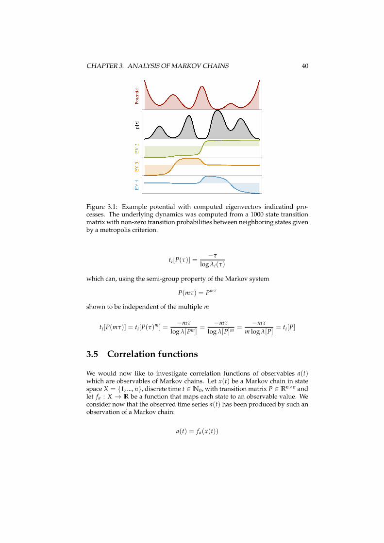
Fig. 3.1 shows an example of the relation between eigenvectors and the under-lying dynamics.
3.4 Timescales and timescale test
The eigenvalues λi are related to a timescale in the manner, that the processvanishes with increasing t slower or faster. Compare the discrete-time decayλt
i and compare it to the exponential decay in continuous time with timescaleti, exp(−t/ti):
λti = exp(−t/ti)
ti =−1
log λi
and if we associate the transition matrix with a real time step τ then then wehave the implied timescales
CHAPTER 3. ANALYSIS OF MARKOV CHAINS 40
Figure 3.1: Example potential with computed eigenvectors indicatind pro-cesses. The underlying dynamics was computed from a 1000 state transitionmatrix with non-zero transition probabilities between neighboring states givenby a metropolis criterion.
ti[P(τ)] =−τ
log λi(τ)
which can, using the semi-group property of the Markov system
P(mτ) = Pmτ
shown to be independent of the multiple m
ti[P(mτ)] = ti[P(τ)m] =
−mτ
log λ[Pm]=
−mτ
log λ[P]m=
−mτ
m log λ[P]= ti[P]
3.5 Correlation functions
We would now like to investigate correlation functions of observables a(t)which are observables of Markov chains. Let x(t) be a Markov chain in statespace X = 1, ..., n, discrete time t ∈ N0, with transition matrix P ∈ R
n×n andlet fa : X → R be a function that maps each state to an observable value. Weconsider now that the observed time series a(t) has been produced by such anobservation of a Markov chain:
a(t) = fa(x(t))
CHAPTER 3. ANALYSIS OF MARKOV CHAINS 41
As a shorthand notation we also define a vector a = ( fa(1), ..., fa(n))T contain-ing the observable of each state of X in the corresponding entry, i.e. we canwrite in short:
a(t) = ax(t)
The autocorrelation function of a(t) can then be written as:
E(a(t) a(t + τ)) = E(ax(t)ax(t+τ)) = ∑i,j∈X
P(x(t) = i, x(t + τ) = j) ai aj
where τ ∈ N0 is a discrete time lag. In the stationary and ergodic case this isequivalent to:
E(a(t) a(t + τ)) = limT→∞
1
T − τ
T−τ
∑t=0
a(t) a(t + τ)
We notice that we can rewrite:
E(a(t) a(t + τ)) = ∑i,j∈X
P(x(t) = i, x(t + τ) = j) ai aj
= ∑i,j∈X
πi pij(τ) ai aj
= aTΠPτa
Using spectral decomposition we can rewrite this as:
E(a(t) a(t + τ)) =n
∑i=1
λτi aTΠrir
Ti Πa
=n
∑i=1
λτi aTlil
Ti a
=n
∑i=1
λτi 〈a, li〉2
=n
∑i=1
λτi γi
with the choice γi = 〈a, li〉2. Thus, we can explain correlation functions interms of multi-exponential decays with timescales/rates given by the eigen-values and intensities depending on the overlap of the observable a with theeigenvectors. On the other hand, we can estimate E(a(t) a(t + τ)) from giventrajectory and explore its spectral properties by observing this multiexponen-tial decay over τ.

CHAPTER 3. ANALYSIS OF MARKOV CHAINS 42
Further Reading:
• Timescales [4]
Chapter 4
Continuous Randomvariables
We now consider continuous random variables. The basic object is as usuala probability space (Ω, Σ, P), which describes the randomness in our experi-ment. Ω is the set of basic samples that can occur, the algebra Σ is the set ofall possible events that we are interested in characterizing. P is a probabilitymeasure that assigns a probability to each event S ∈ Σ. Since we are aimingat continuous random variables, a useful sample space is Ω = R, and a usefulalgebra is the Borel algebra:
Borel algebra is the smallest σ-algebra on the real numbers R. It contains allintervals on the real axis, i.e.:
ix1,x2 = [x1, x2] | x1 ≤ x2; x1, x2 ∈ R ∪ R ∪ ∅
The probability measure P is a measure with the normalization condition P(Ω) =1. A common measure for continuous spaces is the Lebesque measure µ, whichcan be turned into a probability measure by normalizing with µ(Ω):
Lebesque measure is the ordinary notion of length, area, volume of subsetsof Euclidean spaces.
Example: It is useful to think of the probability space as a model for a computerthat generates high-quality random variables (high quality here means almostuncorrelated). Computational random number generators usually have a sam-ple space Ω = [0, 1] ⊂ R, the corresponding algebra is a Borel algebra on thesubset [0, 1] and the probability is given by the normalized Lebesque measure:
P([x1, x2]) =∫ x2
x=x1dx/
∫ 1x=0 dx.
43
CHAPTER 4. CONTINUOUS RANDOM VARIABLES 44
4.1 Continuous random variables
Random variable (continuous) A measurable function X : Ω → R betweena probability space (Ω, Σ, P) and a measurable space (R,B(R)), where B(R)is the Borel-Algebra of R, is a continuous random variable.
Measurable function Definition (measurable function): When (Ω1, Σ1) and(Ω2, Σ2) are measurable spaces, a function f : Ω1 → Ω2 is (Σ1, Σ2)-measureableif
f−1(E2) := ω ∈ Ω1 : f (ω) ∈ E2 ∈ Σ1 ∀E2 ∈ Σ2
Lebesgue Integration A measure space (Ω, Σ, µ) is associated with the the-ory of Lebesgue integration. Let g : Ω → R be a measurable function, then theintegral is defined as:
G :=∫
Ωg dµ =
∫
Ωg(ω) dµ(ω)
In the “nice” case that the measure is absolutely continuous we can rewrite thisin terms of the ordinary Riemann integration
G =∫
Ωg(ω) µ(ω) dω
Probability density function In probability theory, a probability density func-tion (abbreviated as pdf, or just density) of a continuous random variable is afunction that describes the relative likelihood for this random variable to occurat a given point in the observation space. The probability of a random variablefalling within a given set is given by the integral of its density over the set.
A probability density function is most commonly associated with continuousunivariate distributions. A random variable X has density f , where f is a non-negative Lebesgue-integrable function, if:
P[a ≤ X ≤ b] =∫ b
adµ(x) =
∫ b
af (x) dx.
CHAPTER 4. CONTINUOUS RANDOM VARIABLES 45
Cumulative distribution function Hence, if F is the cumulative distributionfunction of X, then:
F(x) =∫ x
−∞f (u) du,
and
f (x) =d
dxF(x).
Intuitively, one can think of f (x)dx as being the probability of X falling withinthe infinitesimal interval [x, x + dx].
Example: As in the example above, consider the probability space of a com-puter that generates [0, 1] random variables with normalized Lebesque mea-sure, ([0, 1],B([0, 1]), µ/µ([0, 1])). We define a random variable x ∈ R whichwe want to be distributed according to f (x). This can be realized by definingx = F−1(ω).
4.2 Properties of Random Variables X ∈ R
Moments: expectation, variance, covariance If f is a probability density func-tion, then the value of the following integral above is called the nth moment ofthe probability distribution.
µn = E(xn) =∫ ∞
−∞xn f (x) dx
For any two random variables X, Y it holds that
µ1(X + Y) = E(X + Y) =∫ ∫
x f (x) y g(y) dx dy = E(X) + E(Y)
The properties discussed for discrete random variables can be transferred tothe continuous case likewise.
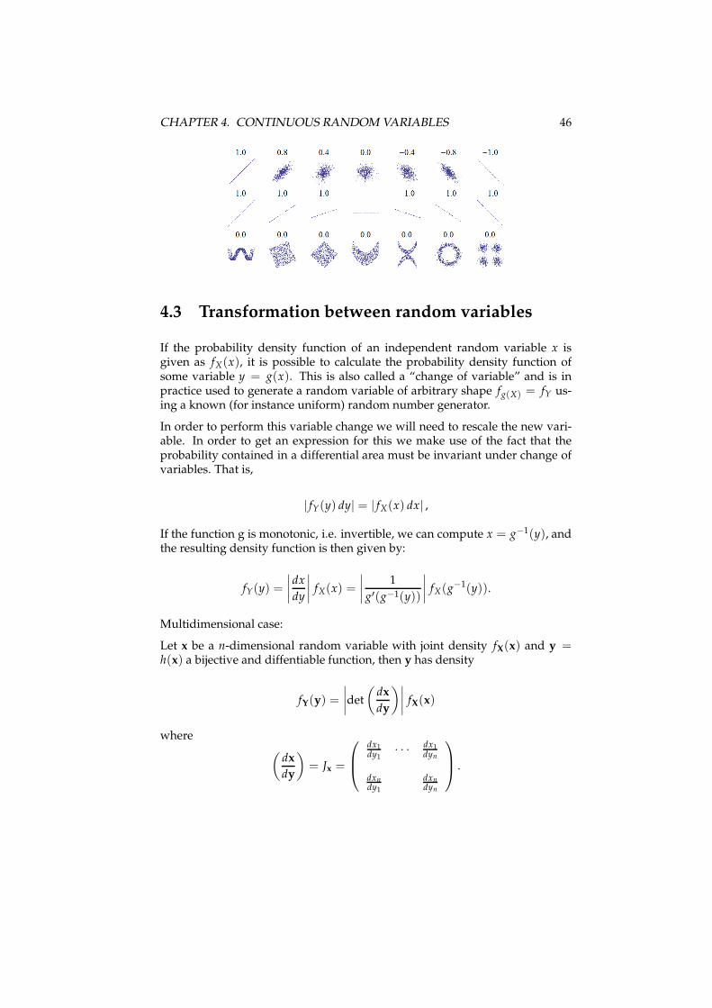
Correlations Consider the following distributions of two random variablesand their correlation coefficients:
CHAPTER 4. CONTINUOUS RANDOM VARIABLES 46
4.3 Transformation between random variables
If the probability density function of an independent random variable x isgiven as fX(x), it is possible to calculate the probability density function ofsome variable y = g(x). This is also called a “change of variable” and is inpractice used to generate a random variable of arbitrary shape fg(X) = fY us-ing a known (for instance uniform) random number generator.
In order to perform this variable change we will need to rescale the new vari-able. In order to get an expression for this we make use of the fact that theprobability contained in a differential area must be invariant under change ofvariables. That is,
| fY(y) dy| = | fX(x) dx| ,
If the function g is monotonic, i.e. invertible, we can compute x = g−1(y), andthe resulting density function is then given by:
fY(y) =
∣∣∣∣
dx
dy
∣∣∣∣
fX(x) =
∣∣∣∣
1
g′(g−1(y))
∣∣∣∣
fX(g−1(y)).
Multidimensional case:
Let x be a n-dimensional random variable with joint density fX(x) and y =h(x) a bijective and diffentiable function, then y has density
fY(y) =
∣∣∣∣det
(dx
dy
)∣∣∣∣
fX(x)
where(
dx
dy
)
= Jx =
dx1dy1
· · · dx1dyn
dxndy1
dxndyn
.
CHAPTER 4. CONTINUOUS RANDOM VARIABLES 47
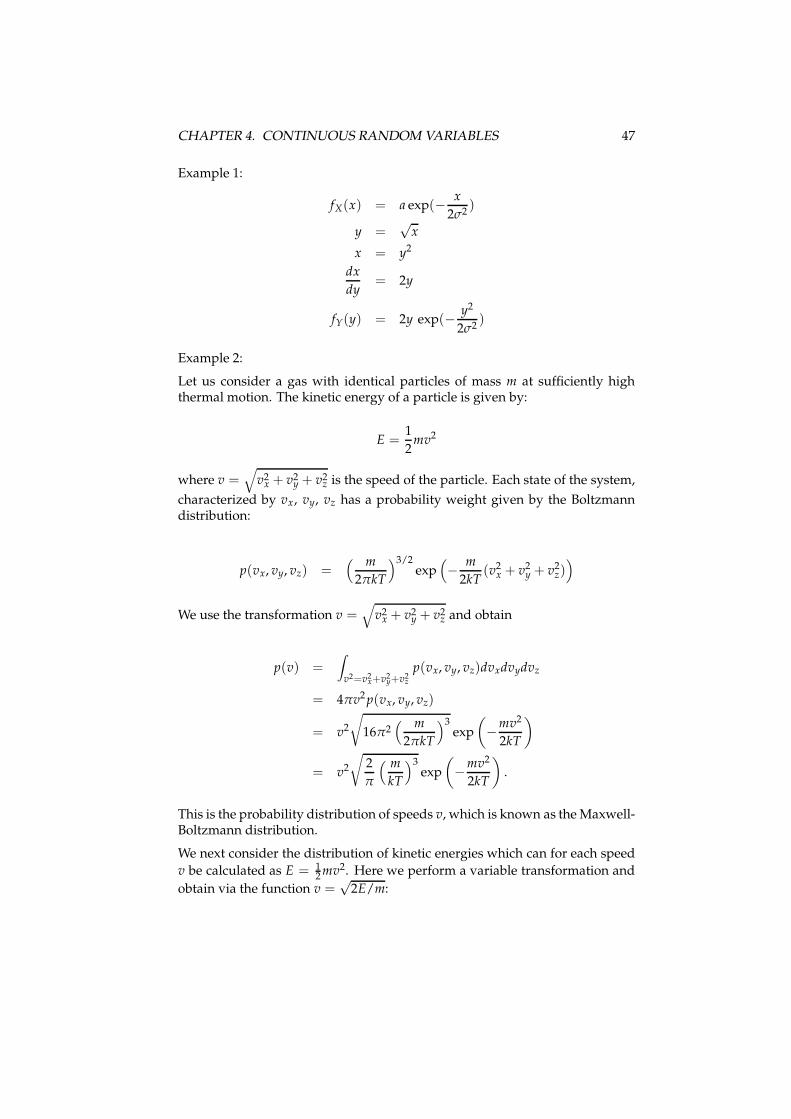
Example 1:
fX(x) = a exp(− x
2σ2)
y =√
x
x = y2
dx
dy= 2y
fY(y) = 2y exp(− y2
2σ2)
Example 2:
Let us consider a gas with identical particles of mass m at sufficiently highthermal motion. The kinetic energy of a particle is given by:
E =1
2mv2
where v =√
v2x + v2
y + v2z is the speed of the particle. Each state of the system,
characterized by vx, vy, vz has a probability weight given by the Boltzmanndistribution:
p(vx, vy, vz) =( m
2πkT
)3/2exp
(
− m
2kT(v2
x + v2y + v2
z))
We use the transformation v =√
v2x + v2
y + v2z and obtain
p(v) =∫
v2=v2x+v2
y+v2z
p(vx, vy, vz)dvxdvydvz
= 4πv2 p(vx, vy, vz)
= v2
√
16π2( m
2πkT
)3exp
(
−mv2
2kT
)
= v2
√
2
π
( m
kT
)3exp
(
−mv2
2kT
)
.
This is the probability distribution of speeds v, which is known as the Maxwell-Boltzmann distribution.
We next consider the distribution of kinetic energies which can for each speed
v be calculated as E = 12 mv2. Here we perform a variable transformation and
obtain via the function v =√
2E/m:
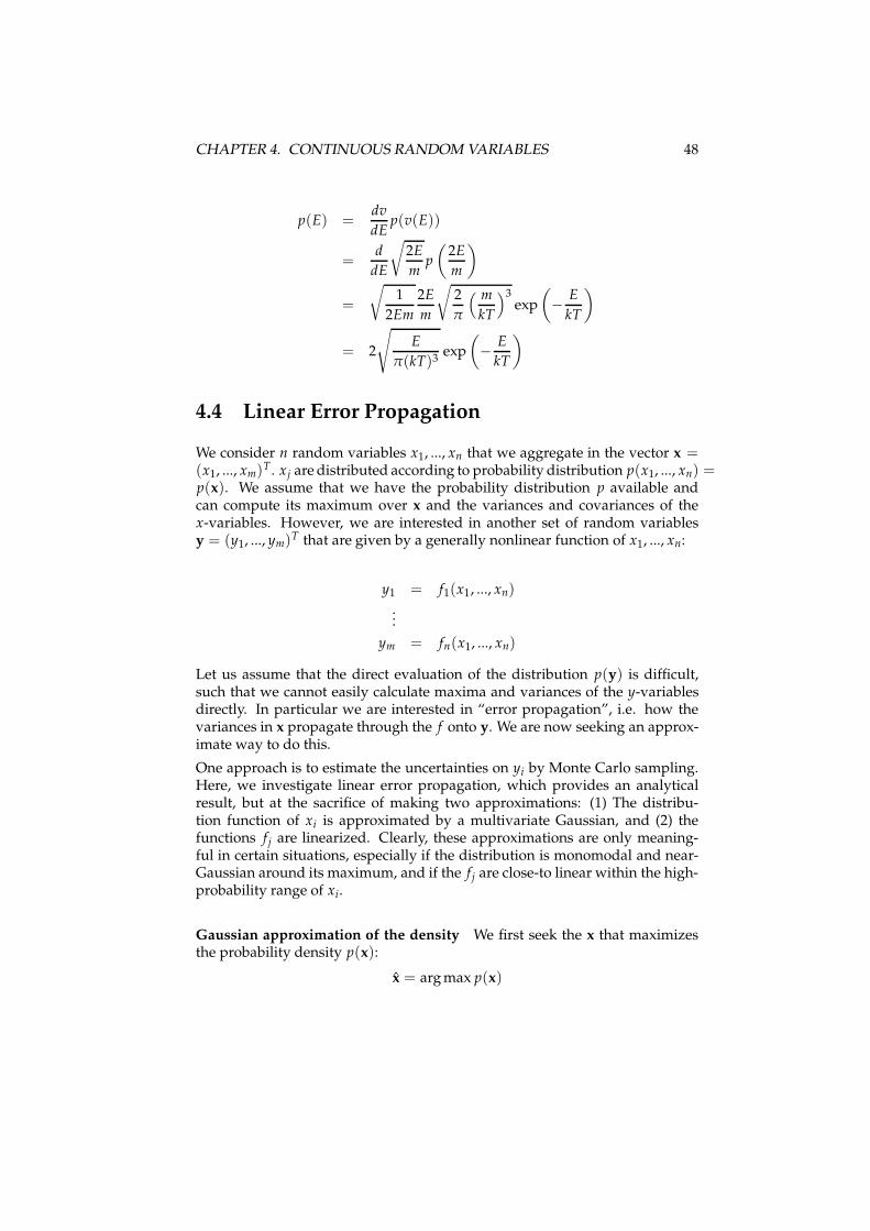
CHAPTER 4. CONTINUOUS RANDOM VARIABLES 48
p(E) =dv
dEp(v(E))
=d
dE
√
2E
mp
(2E
m
)
=
√
1
2Em
2E
m
√
2
π
( m
kT
)3exp
(
− E
kT
)
= 2
√
E
π(kT)3exp
(
− E
kT
)
4.4 Linear Error Propagation
We consider n random variables x1, ..., xn that we aggregate in the vector x =(x1, ..., xm)T . xj are distributed according to probability distribution p(x1, ..., xn) =p(x). We assume that we have the probability distribution p available andcan compute its maximum over x and the variances and covariances of thex-variables. However, we are interested in another set of random variablesy = (y1, ..., ym)T that are given by a generally nonlinear function of x1, ..., xn:
y1 = f1(x1, ..., xn)
...
ym = fn(x1, ..., xn)
Let us assume that the direct evaluation of the distribution p(y) is difficult,such that we cannot easily calculate maxima and variances of the y-variablesdirectly. In particular we are interested in “error propagation”, i.e. how thevariances in x propagate through the f onto y. We are now seeking an approx-imate way to do this.
One approach is to estimate the uncertainties on yi by Monte Carlo sampling.Here, we investigate linear error propagation, which provides an analyticalresult, but at the sacrifice of making two approximations: (1) The distribu-tion function of xi is approximated by a multivariate Gaussian, and (2) thefunctions f j are linearized. Clearly, these approximations are only meaning-ful in certain situations, especially if the distribution is monomodal and near-Gaussian around its maximum, and if the f j are close-to linear within the high-probability range of xi.
Gaussian approximation of the density We first seek the x that maximizesthe probability density p(x):
x = arg max p(x)
CHAPTER 4. CONTINUOUS RANDOM VARIABLES 49
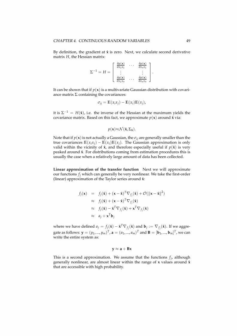
By definition, the gradient at x is zero. Next, we calculate second derivativematrix H, the Hessian matrix:
Σ−1 = H =
∂p(x)∂x1x1
· · · ∂p(x)∂xnx1
......
∂p(x)∂x1xn
· · · ∂p(x)∂xnxn
.
It can be shown that if p(x) is a multivariate Gaussian distribution with covari-ance matrix Σ containing the covariances:
σij = E(xixj)− E(xi)E(xj),
it is Σ−1 = H(x), i.e. the inverse of the Hessian at the maximum yields thecovariance matrix. Based on this fact, we approximate p(x) around x via:
p(x)≈N (x, Σx).
Note that if p(x) is not actually a Gaussian, the σij are generally smaller than thetrue covariances E(xixj) − E(xi)E(xj). The Gaussian approximation is onlyvalid within the vicinity of x, and therefore especially useful if p(x) is verypeaked around x. For distributions coming from estimation procedures this isusually the case when a relatively large amount of data has been collected.
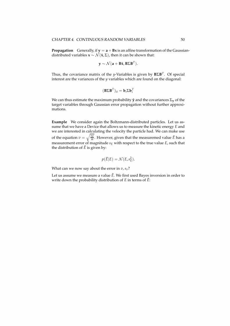
Linear approximation of the transfer function Next we will approximateour functions f j which can generally be very nonlinear. We take the first-order(linear) approximation of the Taylor series around x:
f j(x) = f j(x) + (x − x)T∇ f j(x) +O(‖x − x‖2)
≈ f j(x) + (x − x)T∇ f j(x)
≈ f j(x)− xT∇ f j(x) + xT∇ f j
(x)
≈ aj + xTbj
where we have defined aj = f j(x)− xT∇ f j(x) and bj := ∇ f j
(x). If we aggre-
gate as follows: y = (y1, ..., ym)T, a = (a1, ..., am)T and B = [b1, ..., bm]T, we canwrite the entire system as:
y ≈ a + Bx
This is a second approximation. We assume that the functions f j, althoughgenerally nonlinear, are almost linear within the range of x values around xthat are accessible with high probability.
CHAPTER 4. CONTINUOUS RANDOM VARIABLES 50
Propagation Generally, if y = a+Bx is an affine transformation of the Gaussian-distributed variables x ∼ N (x, Σ), then it can be shown that:
y ∼ N (a + Bx, BΣBT).
Thus, the covariance matrix of the y-Variables is given by BΣBT . Of specialinterest are the variances of the y variables which are found on the diagonal:
(BΣBT)ii = biΣbTi
We can thus estimate the maximum probability y and the covariances Σy of thetarget variables through Gaussian error propagation without further approxi-mations.
Example We consider again the Boltzmann-distributed particles. Let us as-sume that we have a Device that allows us to measure the kinetic energy E andwe are interested in calculating the velocity the particle had. We can make use
of the equation v =√
2Em . However, given that the measuremed value E has a
measurement error of magnitude sE with respect to the true value E, such thatthe distribution of E is given by:
p(E|E) = N (E, s2E).
What can we now say about the error in v, sv?
Let us assume we measure a value E. We first used Bayes inversion in order towrite down the probability distribution of E in terms of E:
CHAPTER 4. CONTINUOUS RANDOM VARIABLES 51
p(E|E) ∝ p(E)p(E|E)
∝1
2πs2E
exp
(
− (E − E)2
2s2E
)
2
√
E
π(kT)3exp
(
− E
kT
)
∝√
E exp
(
− E
kT
)
exp
(
− (E − E)2
2s2E
)
∝√
E exp
(
− (E − E)2kT + 2s2EE
2s2EkT
)
∝√
E exp
(
−E2kT − 2(EkT − s2E)E + E2kT
2s2EkT
)
∝√
E exp
−
(√
kTE − (EkT−s2E)√
kT)2 − (EkT−s2
E)2
kT + E2kT
2s2EkT
∝√
E exp
− (E − (EkT−s2E)
kT )2
2s2E
We abbreviate mE =(EkT−s2
E)kT and obtain:
dp(E|E)dE
=
(
1
2√
E−
√E
s2E
(E − mE)
)
exp
(
− (E − mE)2
2s2E
)
which becomes zero for:
E = arg max p(E|E) =mE ±
√
m2E + 2s2
E
2
of which we choose the positive solution:
E =mE +
√
m2E + 2s2
E
2.
Note that for vanishing error E = mE = E.
The variance of E in a Gaussian approximation around E is given by the inverse
second derivative at E. Using the abbreviation α =√
m2E + 2s2
E, we obtain:
CHAPTER 4. CONTINUOUS RANDOM VARIABLES 52
σ2E =
(d2 p(E|E)
dE2
∣∣∣∣E
)−1
=s2
E
√2mE + 2α
2 exp(− (α−mE)2
8s2E
)α
Thus, we have approximated:
p(E|E) ≈ N (E, σ2E).
Now we use the equation v =√
2Em which is linearized by:
v(E) ≈√
2E
m+
√
1
2mE(E − E)
≈√
2E
m−√
E
2m+
√
1
2mEE
≈√
E
(√
2
m−√
1
2m
)
+
√
1
2mEE
And hence
σ2v =
(dv
dE
)2
σ2E =
s2E
√2mE + 2α
2m(mE + α) exp(− (α−mE)2
8s2E
)α
if we take m = 1 unitless then
σ2v =
s2E√
2mE + 2α exp(− (α−mE)2
8s2E
)α
For small errors sE, this is approximately:
σ2v ≈ s2
E
2E3/2
4.5 Characteristic Functions
An alternative way to represent a probability density fX(x) is by its Fouriertransform. This is called characteristic Function G(ω), defined for all ω ∈ R:
CHAPTER 4. CONTINUOUS RANDOM VARIABLES 53
G(ω) = G(ω)x = E[eiωx] =∫
eiωx fX(x) dx
This is also the moment generating function of the distribution because its Tay-lor expansion turns out to be
G(ω) =∞
∑m=0
(iω)m
m!µm = 1 + iωµ − 1
2ω2µ2 + ...
with the moments µm.
The characteristic function completely determines the behavior and propertiesof the probability distribution of the random variable X. The two approachesare equivalent in the sense that knowledge of one of the functions can alwaysbe used in order to find the other one, yet they both provide different insightfor understanding the features of our random variable. However, in particularcases, there can be differences in whether these functions can be represented asexpressions involving simple standard functions.
If a random variable admits a density function, then the characteristic functionis its dual, in the sense that each of them is a Fourier transform of the other.
Proof of the central limit theorem For a theorem of such fundamental im-portance to statistics and applied probability, the central limit theorem hasa remarkably simple proof using characteristic functions. It is similar to theproof of a (weak) law of large numbers. For any random variable, Xi, withzero mean, the characteristic function of Xi is, by Taylor’s theorem,
G(ω) = 1 − σ2ω2
2+ o(ω2)
where o(ω2) is "little o notation" for some function of ω that goes to zero morerapidly than ω2. Thus, the characteristic function of Zn is
G(ω)Zn = G(ω)
n
∑i=1
Xi
=n
∏i=1
G
(ω√
n
)
Xi
=
[
1 − σ2ω2
2n+ o
(ω2
n
)]n
→ e−ω2σ2/2, n → ∞.
Chapter 5
Markov chain estimation
5.1 Bayesian Approach
Bayes Theorem: Consider two events A and B. Based on the definition of theconditional probability we can follow:
P (A | B) =P(A ∩ B)
P(B)
=
P(A∩B)P(A)
· P(A)
P(B)
=P (B | A) · P(A)
P (B).
Let us consider a model M and observation O. Bayes’ rule states that:
P(M | O) = P(M)P(O | M)
P(O)
in particular, when we consider only one given observation O, we can state:
P(M | O) ∝ P(M) P(O | M).
where we call
P(M | O) posterior probabilityP(M) prior probability of the model MP(O) prior probability of the data O
P(O | M) likelihood
54
CHAPTER 5. MARKOV CHAIN ESTIMATION 55
since usually we only work with a given dataset P(O) is constant, and it issufficient to know that:
P(M | O) ∝ P(M) P(O | M)
The likelihood P(O | M) is usually easy to compute if we have specified thetype of model and we have the data at hand. The prior P(M) is a probabilitythat has the function to bias the estimator towards models that are reasonable.If no prior is used that is equivalent to using a uniform prior, which may notalways be a good choice. Choosing P(M) is a modeling problem, so there is“right” or “wrong” here and it must be chosen with expertise for the processobserved. The significance of the prior is to be able to have a well-defined prob-ability distribution even in the case that no or almost no data is at hand. Whenmore and more data is collected, the likelihood P(O | M) will get sharper andthus eventually dominate the prior. Thus, it is generally a good idea to use arather weak prior that rules out unphysical results but can be easily overcomewhen some data is collected.
When seeking optimial models we will maximize the posterior:
P(M | O) → max
or alternatively we can draw samples xk from it, e.g. with a MCMC approach:
xk ∼ P(M | O)
5.2 Transition Matrix Estimation from Observations;
Likelihood
We consider an observed sequence x(t) ∈ X, t = 0, ..., T in a state spaceX = 1, ..., n.
We assuming that x(t) has been generated from a Markov chain with transitionmatrix P, which we would like to infer from the data. This is a very commonproblem in many applications, such as finance, game theory, molecular physicsand biology.
Let the frequency matrix Z = (zij) ∈ Rn×n count the number of observed
transitions between states, i.e. zij is the number of observed transitions fromstate i at time t to state j at time t + 1, summed over all times t:
zij = |x(t) = i, x(t + 1) = j | t = 0...T − 1|.
CHAPTER 5. MARKOV CHAIN ESTIMATION 56
It is easy to treat the case of observing multiple sequences x(1)(t), ..., x(N)(t) by
noticing that their count matrices add up: Z = Z(1)+ ...+Z(N). As a shorthandnotation we define:
zi :=n
∑k=1
zik.
is the total number of observed transitions leaving state i. It is intuitively clearthat in the limit of an infinitely long trajectory, the elements of the true transi-tion matrix are given by the trivial estimator:
pij =zij
∑k zik=
zij
zi, (5.1)
For a trajectory of limited length, the underlying transition matrix P cannot beunambiguously computed. The probability that a particular P would generatethe observed trajectory x(t) is given by:
P(x(0), ..., x(T) | P) =T−1
∏t=0
px(t),x(t+1) = P(Z|P) =n
∏i,j=1
pzij
ij
Vice versa, the probability that the observed data was generated by a particulartransition matrix P is
P(P|Z) ∝ P(P)P(Z|P) = P(P)n
∏i,j=1
pzij
ij , (5.2)
where P(P) is the prior probability of transition matrices before observing anydata. P(Z|P) is called likelihood. Transition matrix estimation is often ap-proached by identifying the maximum of P(Z|P), i.e., the maximum likelihoodestimator. For the case of a uniform prior, this is identical to the transition ma-trix with maximum posterior probability. Otherwise, we now restrict ourselvesto prior distributions which are conjugate to the likelihood (“conjugate prior”),i.e. have the same functional form. This leads to:
P(P|Z) ∝ ∏i,j
pbij+zij
ij = ∏i,j
pcij
ij , (5.3)
with the prior count matrix B = [bij] and we have defined the total (posterior)number of counts C = B + Z. In the following we will always work with C.The likelihood estimation C = Z is a special case.
CHAPTER 5. MARKOV CHAIN ESTIMATION 57
5.3 Maximum Probability Estimator
We will now derive the Maximum Probability Estimator by finding the tran-sition matrix that maximizes P(P|Z). The probability is difficult to work withdue to the product. For optimization purposes it is therefore a common “trick”to instead work with the logarithm of the likelihood (log-likelihood):
Q = log P(P|C) = ∑i,j
cij log pij.
This is useful since the logarithm is a monotonic function: as a result, the maxi-mum of log f is also the maximum of f . However, this function is not boundedfrom above, since for pij → ∞, Q → ∞. Of course, we somehow need to restrictourselves to sets of variables which actually form transition matrices, i.e., theysatisfy the constraint:
∑j
pij = 1.
When optimizing with equality constraints, one uses Langrangian multipliers.The Lagrangian for Q is given by:
F = Q + λ1(∑j
p1j − 1) + ... ++λm(∑j
pmj − 1).
This function is maximized by the maximum likelihood transition matrix. Itturns out that F only has a single stationary point, which can be easily foundby setting the partial derivatives to zero. Those are given by
∂ log F
∂pij=
cij
pij+ λi.
Set to 0:
cij
pij+ λi = 0
λi pij = −cij.
We now make use of the transition matrix property:
λi
m
∑j=1
pij = λi = −m
∑j=1
cij = −ci
CHAPTER 5. MARKOV CHAIN ESTIMATION 58
and thus:
cij
pij− ci = 0
pij =cij
ci.
It turns out that P(τ), as provided by Eq. (5.1), is the maximum of P(C|P)and thus also of P(P|C) when transition matrices are assumed to be uniformlydistributed a priori. In the limit of infinite sampling, P(P|C) converges towardsa delta distribution with its peak at P(τ).
5.4 Maximum Likelihood Estimator of Reversible
Matrices
It will turn out that in particular when estimating conformation dynamics fromshort trajectories, it is essential to additionally require that the transition matrixis reversible. The reason is that the system itself is in equilibrium, and a statis-tical model for the equilibrium case is desired, but the individual trajectoriesare far off equilibrium, as they are too short to be considered “relaxed” on thetimescale of the molecule. George Boxer (Princeton) has suggested the follow-ing way to compute the maximum likelihood reversible transition matrix:
Let xij = πi pij be the unconditional transition probabilities with the additionalconstraint that ∑i,j xij = 1, the detailed balance condition is given by
xij = xji.
The transition probabilities are given in terms of xij as:
pij =xij
∑nk=1 xik
,
such that the log-likelihood is given by:
and then our goal is to find X = (xji) in order to maximize
Q =m
∑i,j=1
cij
(
log xij − log
(m
∑k=1
xik
))
.
The partial derivatives are given by:
CHAPTER 5. MARKOV CHAIN ESTIMATION 59
∂Q
∂xij=
cij
xij+
cji
xji−
m
∑j′=1
cij′
∑mk=1 xik
−m
∑j′=1
cjj′
∑mk=1 xjk
and writing ci = ∑nk=1 cki and xi = ∑
nk=1 xki we have
∂Q
∂xji=
cji + cij
xji− ci
xi− cj
xj
When Q is maximized ∂Q∂x ji
= 0 and so this gives the condition that
xji =cij + cji
cixi+
c j
x j
and we can iterate this condition to convergence.
5.5 Error Propagation
We start again with the posterior distribution of transition matrix P ∈ Rn×n:
P(P|Z) ∝ ∏i,j
pcij
ij , (5.4)
setting U = (uij) = (cij + 1), we can rewrite this as:
P(P|Z) ∝ ∏i
∏j
puij−1
ij = ∏i
Dir (pi, ui)
where Dir is a Dirichlet distribution, a well-known distribution. Based onknown properties of this distribution we can state using the abbreviation ui =∑j uij:
pij = [E(P)]ij =uij
ui=
cij + 1
ci + n
pij = [P]ij = (arg max P(P|Z))ij =uij − 1
uij − n=
cij
ci
Var(pij) =uij(ui − uij)
u2i (ui + 1)
=pij(1 − pij)
(ui + 1)=
pij(1 − pij)
ci + n + 1
Cov(pij, pik) =−uijuik
u2i (ui + 1)
∀i 6= j
CHAPTER 5. MARKOV CHAIN ESTIMATION 60
We now are interested in the question how the uncertainties given by Var(pij)propagate onto uncertainties of functions derived from transition matrices,such as eigenvalues. If we do not use constraints between different rows suchas detailed balance, the rows can be treated as independent sets of randomvariables and thus:
Cov(
pij, plk
)= 0, i 6= l
We can thus define a Covariance matrix separately for each row as:
Σ(i)jk := Cov
(pij, pik
)=
1
u2i (ui + 1)
[
uiδjkuij − uijuik
]
=1
(ui + 1)
[
δjk pij − pij pik
]
where δ is the Kronecker delta. Alternatively, we can write the covariance ma-trix in vector notation:
Σ(i) =1
(ui + 1)
[
diag ( pi)− pi pTi
]
This means, that the covariance for the Dirichlet processes scales with the totalnumber of count in a row.
Using this first two moments of the distribution we can approximate each rowin the transition matrix Pi by a multivariate Gaussian distribution of the form
Pi ∼ N(
pi, Σ(i))
This we can use in Gaussian error propagation for linear functions of the tran-sition matrix (see above). Let us assume we have a scalar function f (P) :R
n×n → R. The first order Taylor approximation is given by:
f (P) = f (P) +∑i,j
∂ f
∂pij
(P)(pij − pij).
Since we know that the rows are independent we define a sensitivity vector foreach row separately
s(i)j =
∂ f
∂pij(P)
CHAPTER 5. MARKOV CHAIN ESTIMATION 61
and with the function for the error propagation we get
f = f(
P)
and
Var ( f ) = Cov( f , f ) = ∑i
(
s(i))T
Σ(i)s(i)
Example: Eigenvalues For properly normalized eigenvectors we have:
Λ = LPR
λ(k) = l(k)Pr(k)
= ∑i,j
l(k)i pijr
(k)j
∂λ(k)
∂pij= l
(k)i r
(k)j
and for unnormlized eigenvectors this is corrected by:
∂λ(k)
∂pij=
l(k)i r
(k)j
〈l(k), r(k)〉
and thus, using the linear perturbation approach:
Var(
λ(k))
=n
∑i=1
∑a,b
∂λ(k)
∂piaCov(pab)
∂λ(k)
∂pib
=1
〈l(k), r(k)〉2
n
∑i=1
∑a,b
l(k)i r
(k)a
(
∑a
uia(ui − uia)
u2i (ui + 1)
+ ∑a,b 6=a
−uiauib
u2i (ui + 1)
)
l(k)i r
(k)b
In the special case of p = 1 we have li = πi, ri = 1 with l · r = 1 and we get
CHAPTER 5. MARKOV CHAIN ESTIMATION 62
Var(
λ(1))
=n
∑i=1
∑a 6=b
∂λ(k)
∂piaVar(p
(i)aa )
∂λ(k)
∂pia+ ∑
a 6=b
∂λ(k)
∂piaCov(p
(i)ab )
∂λ(k)
∂pib
=n
∑i=1
π2i
(
∑a
uia(ui − uia)
u2i (ui + 1)
+ ∑a,b 6=a
−uiauib
u2i (ui + 1)
)
=n
∑i=1
π2i
u2i (ui + 1)
(
∑a 6=b
uiaui − uiauia − ∑a,b 6=a
uiauib
)
=n
∑i=1
π2i
u2i (ui + 1)
(
ui ∑a
(uia − uia)
)
= 0
which is the expected result, since the first eigenvalue is constant.
The limitation of this approach is that it does not work well in situations wherethe Transition matrix distribution is far from Gaussian (especially in the situa-tion of little data). Furthermore, the more nonlinear a given function of interestis in terms of pij, the more the estimated uncertainty on this function might bewrong.
Further Reading:
• Error Estimation [3, 1]
5.6 Full Bayesian Estimation
Here, a general method to sample transition matrices according to the posteriorprobability (5.3) based on Markov Chain Monte Carlo (MCMC) is proposed.While it is computationally more expensive than the linear error analysis andthe Dirichlet sampling, it is more general than these methods. In particular,it allows (i) the complete distribution of arbitrary observables to be approxi-mated to the desired degree of accuracy, (ii) the sampling to be restricted totransition matrices fulfilling additional constraints, such as detailed balanceand predefined π, and (iii) arbitrary prior distributions, p(T), to be employed.The method is illustrated on µs MD simulations of a hexapeptide for which thedistributions and uncertainties of the free energy differences between confor-mations, the transition matrix elements and the transition matrix eigenvaluesare estimated.
To sample the distribution 5.3, a sampling procedure is proposed based ontaking Monte-Carlo steps in T-space: Given a current matrix T and a proposednew matrix T′, the acceptance probability is computed by:
CHAPTER 5. MARKOV CHAIN ESTIMATION 63
paccept =p(T′ → T)
p(T → T′)p(T′|C)p(T|C) (5.5)
where p(T → T′) and p(T′ → T) denote the probability to propose T′ givenT and vice versa. Any proposal step can be used to sample the probabilityp(T|C), provided that two conditions are satisfied:
• p(T → T′) and p(T′ → T) can be evaluated for every possible proposalstep, such that (5.5) can be evaluated.
• The proposal steps generate an ergodic chain, i.e. if T denotes the setof matrices to be sampled from, then from any matrix T ∈ T any othermatrix T′ ∈ T must be accessible with a finite number of steps.
MCMC sampling of transition matrices: See paper F. Noé: “Probability Dis-tributions of Molecular Observables computed from Markov Models”, J. Chem.Phys 128, 244103 (2008).
5.6.1 Metropolis-Hastings sampling
We want to sample
p(P|Z) ∝ p(P)p(Z|P) = p(P)∏i,j
pcij
ij (5.6)
where pij is the transition probability from state i to state j and cij are the num-ber of observed transitions in the data set. For the sake of simplicity we assumea uniform prior
p(P|Z) ∝ p(Z|P) = ∏i,j
pcij
ij , (5.7)
however, the use of non-uniform priors is straight forward. Using the Metropolis-Hastings algorithm, we have
pMH =p(P′ → P) p(P′|Z)p(P → P′) p(P|Z) =
p(P′ → P) p(Z|P′)p(P → P′) p(Z|P) =
p(P′ → P) ∏i,j p′cij
ij
p(P → P′) ∏i,j pcij
ij
(5.8)
The goal is to find proposal steps P → P′ and the corresponding proposal prob-ability p(P → P′), such that the proposed transition matrices P′ fulfill certainconstraints, e.g. stochasticitiy, detailed balance or fixed stationary distribution.
CHAPTER 5. MARKOV CHAIN ESTIMATION 64
5.6.2 Non-reversible shift element
Shifts a single off-diagonal element pij of the original transition matrix P by∆. The reverse element pji is not altered and, therefore, detailed balance is notguaranteed. Stochasticity is preserved by an appropriate modification of thediagonal element pii:
p′ij = pij − ∆ (5.9)
p′ii = pii + ∆ , (5.10)
where ∆ is a uniform random number in[−pii, pij
]. The forward and backward
proposal probabilities are symmetric:
p(P → P′) =1
pij + pii(5.11)
p(P′ → P) =1
pij − ∆ + pii + ∆= p(P → P′) . (5.12)
and, thus,
pMH =∏i,j p′
cij
ij
∏i,j pcij
ij
=
(
pij − ∆
pij
)cij (pii + ∆
pii
)cii
(5.13)
5.6.3 Reversible shift element
Shifts a off-diagonal element pij of the original transition matrix P by ∆. Thereverse element pji is altered such that detailed balance
πi pij = πj pji (5.14)
is maintained. Stochasticity is preserved by an appropriate modification of thediagonal elements pii and pjj:
p′ij = pij − ∆ (5.15)
p′ji = pji −πi
πj∆ (5.16)
p′ii = pii + ∆ (5.17)
p′jj = pjj +πi
πj∆ (5.18)
Allowed range of ∆:
CHAPTER 5. MARKOV CHAIN ESTIMATION 65
upper bound:(a) p′ij = pij − ∆ ≥ 0 → ∆ ≤ pij
(b) p′ji = pji − πiπ j
∆ ≥ 0 → ∆ ≤ π j
πipji = pij
lower bound:(c) p′ii = pii + ∆ ≥ 0 → ∆ ≥ −pii
(d) p′jj = pjj +πiπ j
∆ ≥ 0 → ∆ ≥ −π j
πipjj
and thus
∆ ∈[
max
(
−pii,−πj
πipjj
)
, pij
]
. (5.19)
The proposal probability in the forward direction is
p(P → P′) =1
pij − max(
−pii,−π j
πipjj
) (5.20)
and in the backward direction
p(P′ → P) =1
p′ij − max(
−p′ii,−π j
πip′jj)
, p′ij(5.21)
=1
pij − ∆ − max(
−pii − ∆,−π j
πi(pjj +
πiπ j
∆)) (5.22)
=1
pij − ∆ − max(
−pii − ∆,−π j
πipjj − ∆
) (5.23)
= P(P → P′) . (5.24)
The accepting probability is
pacc = min1, pMH (5.25)
(5.26)
pMH =∏i,j p′
cij
ij
∏i,j pcij
ij
=
(
pij − ∆
pij
)cij (pii + ∆
pii
)cii
pji − πiπ j
∆
pji
c ji
pjj +πiπ j
∆
pjj
c jj
(5.27)
If P fulfills detailed balance, the stationary distribution remains unchanged(π′ = π):
πP′ = [π1, ..., πi−1,
π1 p1i + ... + πi(pii + ∆) + ... + πj(pji −πi
πj∆) + ... + πm pmi, πi+1, ..., πj−1,
π1 p1j + ... + πi(pij − ∆) + ... + πj(pjj +πi
πj∆) + ... + πm pmj, πj+1, ..., πm]
= [π1, ..., πm] = π.
CHAPTER 5. MARKOV CHAIN ESTIMATION 66
Furthermore, if P fulfills detailed balance, P′ fulfills detailed balance as well:
π′i p′ij = πi(pij − ∆) = πi pij − πi∆
π′j p
′ji = πj(pji −
πi
πj∆) = πj pji − πi∆
Thus
πi pij = πj pji ⇒ π′i p′ij = π′
j p′ji.
5.6.4 Row Shift
Finally a step is considered which scales the self-transition probability, pii, andall outgoing transition probabilities, pij as follows:
p′ij = αpij
p′ii = 1 − ∑k 6=i
p′ik
= 1 − α ∑k 6=i
pik
= 1 − α(1 − pii)
= αpii − α + 1
The step thus changes the ith row of P. The parameter α is subject to the fol-lowing constraints:
αpij ≥ 0 → α ≥ 0 (a)αpii − α + 1 ≤ 1 → α ≥ 0 (b)αpii − α + 1 ≥ 0 → α ≤ 1
1−Tii(c)
αpij ≤ 1 ∀j 6= i → α ≤ 1max(Tij)
∀j 6= i (d)
Note that (1− pii) ≥ pij for all j 6= i, and thus (1− pii)−1 ≤ (max(pij))
−1, mak-ing (d) redundant with (c). Consequently, α is drawn uniformly from followingrange:
α ∈[
0,1
1 − pii
]
CHAPTER 5. MARKOV CHAIN ESTIMATION 67
The ratio of proposal probabilities is given by:
p(P′ → P)
p(P → P′)=
pα(P′ → P)
pα(P → P′)dA′
dA=
dr′dA′
dr dA,
where pα is the proposal probability along the line parametrized by α, while dAis an area element orthogonal to that line and intersecting with P, and dA′ is thescaled area element. With p(α) = 1 − pii and α = p′ij/pij = (1 − p′ii)/(1 − pii)
we obtain (see paper) pα(P′ → P)/pα(P → P′) = 1. The area element is pro-portial to the (m − 2)nd power of the distance of the ith row from (0, ..., 0, pii =1, 0, ..., 0), denoted by r:
dA ∝ (r · dc)(m−2)
dA′ ∝ (r′ · dc)(m−2).
With r =√
(1 − pii)2 + ∑j 6=i p2ij and r′ =
√
α2(1 − pii)2 + ∑j 6=i α2 p2ij = αr one
obtains:
p(P′ → P)
p(P → P′)= α(m−2).
Acceptance probability:
pacc =p(P′ → P)
p(P → P′)p(P′|C)p(P|C)
= α(m−2)
(p′iipii
)Cii
∏j 6=i
(p′ijpij
)Cij
= α(m−2)
(1 − α(1 − pii)
pii
)Cii
∏j 6=i
αCij
= α(m−2+Ci−Cii)(
1 − α(1 − pii)
pii
)Cii
with Ci = ∑mj=1 Cij.
The row shift operation will change the stationary distribution π. π is, for ex-ample, required to conduct the reversible element shifts. Instead of recomput-ing the stationary distribution expensively by solving an eigenvalue problem,it may be efficiently updated as follows:
CHAPTER 5. MARKOV CHAIN ESTIMATION 68
π′i =
πi
πi + α(1 − πi)
π′j =
απj
πi + α(1 − πi).
Proof:
π′ = π′P′
has the elements πi and πj, j 6= i, given by:
π′i = π′
1 p′1i + ... + π′i−1 p′i−1,i + π′
i p′ii + π′i+1 p′i+1,i + ... + π′
m p′mi
πi
πi + α(1 − πi)=
απ1 p1i + ... + απi−1pi−1,i + πi[1 − α(1 − pii)] + απi+1 pi+1,i + ... + απm pmi
πi + α(1 − πi)
πi = α[π1 p1i + ... + πm pmi] + πi − απi
πi = π1 p1i + ... + πm pmi
and
π′j = π′
1 p′1j + ... + π′i−1 p′i−1,j + π′
i p′ij + π′i+1 p′i+1,j + ... + π′
m p′mj
απj
πi + α(1 − πi)=
απ1 p1j + ... + απi−1 pi−1,j + πiαpij + απi+1 pi+1,j + ... + απm pmj
πi + α(1 − πi)
πj = π1 p1j + ... + πm pmj.
Thus:
π = πP ⇔ π′ = π′P′
Chapter 6
Markov Jump Processes
Time-continuous Markov processes When time steps are taken to be spaceddifferentially small, the above definition is also useful to define time-continuousMarkov processes. For example Brownian motion, Langevin dynamics, andMaster equation dynamics are all time-continuous Markov processes.
Intuitively, one can define a time-homogeneous Markov process as follows. Letx(t) ∈ X = 1, ..., n be the random variable describing the state of the processat time t. Now prescribe that, given that the process starts in a state i at time t, ithas made the transition to some other state j 6= i at time t + h with probabilitygiven by
p(x(t + h) = j | x(t) = i) = kijh + o(h),
where o(h) represents a quantity that goes to zero faster than h goes to zero. Inother words, the limit
limh→0+
dp(x(t+ h) = j | x(t) = i)
dh= lim
h→0+
d
dh(kijh + o(h)) = kij
exists. The transition rates kij, i, j ∈ X defined the transition rate matrix K ∈R
n×n. For the probabilities to be conserved, i.e., the probabilities associatedwith starting in a given state must add up to one, the off-diagonal elements ofK must be non-negative and the diagonal elements must satisfy
kii = −∑j 6=i
kij.
With this notation, and letting pt ∈ Rn the probability to be at any state at time
t, the evolution of a continuous-time Markov process is given by the first-orderdifferential equation
69
CHAPTER 6. MARKOV JUMP PROCESSES 70
d
dtpt = ptK
To see the reason of the definition of kii, we expand this equation out by com-ponents:
d
dtpi(t) =
n
∑j=1
pj(t)kji
=n
∑j 6=i
pj(t)kji + pi(t)kii
=n
∑j 6=i
pj(t)kji
︸ ︷︷ ︸
gain
− ∑j 6=i
pi(t)kij
︸ ︷︷ ︸
loss
.
which is known as the Master equation or gain-loss equation.
The probability that no transition happens in some time r is
P(x(s) = i ∀ s ∈ (t, t + h] | x(t) = i) = ekiih.
That is, the probability distribution of the waiting time until the first transitionis an exponential distribution with rate parameter −kii, and continuous-timeMarkov processes are thus memoryless processes.
A time dependent (time heterogeneous) Markov process is a Markov processas above, but with the k-rate a function of time, denoted kij(t).
6.1 Poisson process
This is an important stochastic process in physics modelling countable, singu-lar events in continuous time, such as:
• The arrival of "customers" in a queue.
• The number of raindrops falling over an area.
• The number of photons hitting a photodetector.
• The number of particles emitted via radioactive decay by an unstablesubstance, where the rate decays as the substance stabilizes.
CHAPTER 6. MARKOV JUMP PROCESSES 71
It is parametrized by a “rate” or “intensity” constant k, or equivalently the char-acteristic timescale τ = k−1. A time-homogeneous Poisson process is definedas a counting process N(t) where the number of counts (N(t + ∆t)− N(t)) inthe time interval (t, t + ∆t] follows a Poisson distribution with parameter k∆t.This relation is given as:
P[(N(t + ∆t)− N(t)) = n] =e−k∆t(k∆t)n
n!n ∈ N0 (6.1)
k is the expected number of events per unit time and τ = k−1 is the expectedduration between two events. It can be shown that the moments of this distri-bution are:
E[n] = k∆t,
i.e. the mean number of counts is simply the waiting time times the rate, andalso
Var[n] = k∆t.
For large enough statistics (∆t ≫ k−1), the central limit theorem makes thePoisson distribution converge towards a Gaussian distribution with correspond-ing moments:
limk∆t→∞
P[(N(t + ∆t)− N(t)) = n] = N (k∆t, k∆t).
For short enough times, the probability to get more than one count in ∆t van-ishes:
limk∆t→0
P[(N(t + ∆t)− N(t)) > 1]
P[(N(t + ∆t)− N(t)) = 1]= lim
k∆t→0
1
e−k∆tk∆t
∞
∑n=2
e−k∆t(k∆t)n
n!
= limk∆t→0
∞
∑n=2
(k∆t)n−1
n!
= 0
Thus in the short-time limit, we can ignore the possibility to get more than onecount:
P[(N(t + ∆t)− N(t)) = 0] = e−k∆t
P[(N(t + ∆t)− N(t)) = 1] = k∆t e−k∆t
P[(N(t + ∆t)− N(t)) > 1] ≈ 0.
CHAPTER 6. MARKOV JUMP PROCESSES 72
for k∆t → 0, we also have e−k∆t ≈ 1 − k∆t
P[(N(t + ∆t)− N(t)) = 0] ≈ 1 − k∆t
P[(N(t + ∆t)− N(t)) = 1] ≈ k∆t(1 − k∆t) ≈ k∆t.
which is identical to a binomial distribution P[(N(t + ∆t) − N(t)) = n] =(k∆t)n(1 − k∆t)1−n for n ∈ 0, 1.
Let us go back to the general case (6.1). Without loss of generality we start theprocess at time t = 0 and ask for the probability of t1, the time at which thefirst count occurs:
dt ft1(t) = P[(N(t1)− N(0) = 0] P[(N(t1 + dt)− N(t1) = 1]
= e−kt1 e−k dtk dt
= dt k e−kt1
Due to the independence of events in subsequent intervals, the probability den-sity of any intermittance time t between two counts is:
ft(t) = k exp(−kt)
=1
τexp
(
− t
τ
)
.
This also shows immediately that the mean waiting time is equal to τ:
E[t] =∫ ∞
t=0ft(t) t dt = τ = k−1
while the variance is
Var[t] = E[t2]− E[t]2 = τ2 = k−2
6.2 Markov Jump Process
Consider a system that can exist in two states such as the chemical reaction:
1k→ 2
CHAPTER 6. MARKOV JUMP PROCESSES 73
and let the time-dependent populations of agents “1” and “2” be denoted byp1(t) and p2(t). We can model their evolution by the following differentialequations
−dp1(t)
dt= kp1(t) =
dp2(t)
dt
Solving for p1:
dp1
p1= −kdt
∫ p1(t)
p1(0)
dp1
p1= −k
∫ t
0dt
lnp1(t)
p1(0)= −kt
p1(t) = p1(0) exp(−kt).
and for p2:
∫ p2(t)
p2(0)dp2(t) = −
∫ p1(t)
p1(0)dp1(t)
p2(t)− p2(0) = p1(0)− p1(t)
p2(t) = p1(0) + p2(0)− p1(0) exp(−kt)
Generally we can say that both time evolutions have the functional form pi(t) ∼exp(−kt), while multiplicative and additive constants can be used to realizedifferent solutions.
Here, p1 and p2 are concentrations or amounts of the corresponding chemicals.Now we change the viewpoint and look at a single copy of molecule 1. We askat which time, t, this copy will decay to molecule 2. Since this decay occurswith a constant rate and independent of the past, it has to be ft(t) ∝ exp(−kt),which normalized becomes:
ft(t) = k exp(−kt),
thus each exit process of a Markov jump process is a Poisson process. In otherwords, a Markov jump process (which can generally consist of many statesthat interconvert), is a superposition of Poisson processes, each occurring witha rate that corresponds to the exit rate out of the current state.
As an example consider C2H6 → 2CH3. This reaction is irreversible and has arate of 5.46 · 10−4s−1 under normal temperature and pressure conditions.
Let us now consider the general case: We have m states (e.g. chemical species),for each of them we consider a concentration, population or probability
pi ∈ R, i ∈ 1, ..., m.
CHAPTER 6. MARKOV JUMP PROCESSES 74
And we have a number of simple reactions between species of the sort
pi
kij→ pj
between some pairs i, j ∈ 1, ..., m. We can formally define all rates
kij ∈ R, i, j ∈ 1, ..., m,
and set those to 0 where no reaction exists.
6.3 Master equation
Now the time evolution of the pi is given by a differential equation with a sumof gains and losses, called Master equation:
dpi
dt= ∑
j 6=i
[kji pj − kij pi
]
= ∑j 6=i
kji pj + pi ∑j 6=i
−kij
= ∑j 6=i
kji pj + kii pi
=m
∑j=1
kji pj
where we have formally defined
kii = ∑j 6=i
−kij,
allowing us to write the Master equation in matrix form simply as:
dpT(t)
dt= pT(t)K.
with generator / rate matrix K ∈ Rm×m containing nonnegative off-diagonal
and nonpositive diagonal entries:
kij ≥ 0 ∀i 6= j
kii = −∑i 6=j
kij ∀i
CHAPTER 6. MARKOV JUMP PROCESSES 75
Note that we have conservation of mass, i.e.
‖p‖1 =m
∑i=1
pi = ptot = const.
Using the normalization convention ptot = 1, we can look at the same equationin terms of moving probability densities:
dp(t)T
dt= p(t)TK.
The Master equation has the following formal solution:
pT(t + τ) = pT(t) exp(Kτ) (6.2)
(of course all constant shifts are also solutions).
This suggests to compare to Markov chains, where we have:
pT(t + τ) = pT(t)T(τ), (6.3)
showing that we have the equivalence:
T(τ) = exp(Kτ). (6.4)
where exp(·) is the Matrix exponential, which is defined as:
exp(Kτ) = exp(τRΛR−1)
= exp(τRdiag(κ1, ..., κm)R−1)
= Rdiag(exp(τκ1), ..., exp(τκm))R−1
whereR = [r1, ...rm]
is the right eigenvector matrix with eigenvectors ri in the columns, and
diag(κ1, ..., κm)
is a diagonal matrix with the eigenvalues κi on the diagonal.
Thus, the transition and the rate matrix are closely related. T(τ) is the prop-agator for the solution of the Master equation for time interval τ. In other
CHAPTER 6. MARKOV JUMP PROCESSES 76
words, Eq. (6.3) is an exact solution of Eq. (6.2) at time points τ, i.e. an ex-act time-discretization. We can compare this to the approximative solution thatis obtained when we make the time step τ very small, such that τκi → 0 ∀i ∈1, ..., m, and exp(τκi) ≈ 1 + τκi ∀i ∈ 1, ..., m:
exp(Kτ) = Rdiag(exp(τκ1), ..., exp(τκm))R−1
≈ Rdiag(1 + τκ1, ..., 1+ τκm)R−1
≈ Id + τK,
which is a first-order Taylor approximation. The resulting equation is
T(τ) ≈ Id + τK
and the associated solution approximation to the Master equation is
pT(t + τ) ≈ pT(t) + τpT(t)K,
which is just the Euler discretization of the Master equation.
Note that the formal inverse operation K = τ−1 log(T(τ)) should be avoided.This operation is numerically very unstable (fluctuations of eigenvalues closeto 0 become strongly amplified by the log), and also T(τ) has a greater real-valued support than K: T(τ) may have negative eigenvalues, in which case noreal-valued solution of the log exists. However the operation
Kp(τ) =T(τ)− I
τ
is always permitted. Kp(τ) ≈ K is called pseudogenerator, and it is an approx-imation to the true rate matrix in a Markov jump process. The approximationbecomes exact in the limit:
K = limτ→0+
T(τ)− I
τ,
and if that limit exists, then the process is said to have the generator K. When infact the underlying process is already a time-discrete Markov chain at some fi-nite time τ, then Kp(τ) is exact and we can treat the Markov chain as a Markovjump process with Kp(τ) as rate matrix.
Due to the close relationship to Markov chains, many properties of Markovchains have direct equivalents for Markov jump processes. If K is irreducibleand positively recurrent it has a stationary distribution given by
CHAPTER 6. MARKOV JUMP PROCESSES 77
0 = πTK.
The backward generator is defined as:
kij =πj
πikji
If K is furthermore reversible it fulfills the detailed balance equation:
kij = kij ∀i, j.
πikij = πjkji ∀i, j.
6.4 Solving very large systems
Consider a situation where state space is huge. For example, in the limit of fewparticles, we would no longer like to use particle concentrations, but wouldlike to resolve particle number. For example, a virus A can replicate with somerate k1, be killed by a drug B with some other rate k2, but the drug also degen-erates with some rate k3:
Ak1→ 2A
A + Bk2→ B
Bk3→ 0
Now we are interested in the question: Given a set of rate constant and the factthat a patient has initially [A] virus particles and receives [B] drug molecules,will the virus be killed, or will it survive? We need to resolve few particlenumbers, because a single surviving virus could spawn a new population, ora single surviving drug can still kill a small population. So the difference be-tween 0 and 1 copies is important and cannot be resolved by a concentration.Now the state space of our system is huge, because each combination of copynumbers of A and B is a state, e.g. [(0,0), (0,1), (1,0), ...]. In principle the statespace is infinite, but even when we limit ourselves to 1000 copies per species atmost (which is only reasonable for certain settings of initial concentrations andrate constants), then we already have 106 states, and we don’t want to makelinear algebra operations with a 106 × 106 rate matrix. Therefore we need away to simulate this system without ever evaluating the entire matrix.
We notice two facts:
CHAPTER 6. MARKOV JUMP PROCESSES 78
1. At a given time t, consider we are in state i. Exit out of this state occurs viaa Poisson process with rate ki = ∑j kij = −kii. This means the lifetime, orwaiting time, τi, is distributed as:
p(τi) = ki exp(−kiτi).
with the cdf
F(τi) = P(τ′i ≤ τi) = ki
∫ τi
0dt exp(−kiτ
′i )
= ki[−1
kiexp(−kiτi) +
1
ki]
= 1 − exp(−kiτi)
whose inverse is:
τi = − ln[1 − F(t0)]
ki
thus, if v is a uniform random variable in [0, 1], then − ln u/ki is dis-tributed as p(t).
2. Given that we in a state i and have two options to leave, using rates k1
and k2, what is the probability to choose 1 versus 2? Call the exit time tostate 1 t2 and to state 2 t2:
P(t1 < t2) =∫ ∞
t=0p(t1 = t) P(t2 > t) dt
=∫ ∞
t=0k1 exp(−k1t) [1 − (1 − exp(−k2t)] dt
=∫ ∞
t=0k1 exp(−k1t) exp(−k2t) dt
=∫ ∞
t=0k1 exp(−t(k1 + k2)) dt
=k1
k1 + k2
and
P(t2 < t1) =k2
k1 + k2.
This argument can be easily extended to more than 2 states.
Based on these two arguments, we can propose an algorithm to sample tra-jectories from rate systems without evaluating the full matrix. The Gillespiealgorithm for simulating the time evolution of a system where some processescan occur with known rates K can be written as follows:
1. Set the time t = 0 and initial state i = i0.
CHAPTER 6. MARKOV JUMP PROCESSES 79
2. Form a list of all possible states that can be reached from the current statei and corresponding rates ki1, ..., kin. Let the total reaction rate be ki =∑
nj=1 kij
3. Calculate the cumulative function pj =∑
js=1 kis
kifor j = 0, . . . , n.
4. Generate a uniform random number u ∈ (0, 1] and find the event to carryout j by finding the j for which pj−1 < u ≤ pj (this can be achievedefficiently using binary search). Update state i
5. Generate a uniform random number v ∈ (0, 1] and update time by t =
t − log vki
6. Return to step 2.
This algorithm is known in different sources variously as the residence-timealgorithm or the n-fold way or the Bortz-Kalos-Liebowitz (BKL) algorithm,Gillespie algorithm, or just the kinetic Monte Carlo (KMC) algorithm. It isimportant to note that the timestep involved is a function of the probabilitythat all events i, did not occur.
6.5 Hitting Probabilities, Committors and TPT fluxes
Similar as for transition matrices, we can derive simply expressions for transi-tion path theory using rate matrices.
Hitting probabilites for Markov Jump Processes Using
hAi = 1for i ∈ A
hAi = ∑
j∈I
pijhAj for i /∈ A.
with K = P − I (The linear expansion is sufficient for solving a linear systemof equations) yields
hAi = 1for i ∈ A
hAi = ∑
j∈I,j 6=i
kijhAj + (kii + 1)hA
i for i /∈ A.
and thus
CHAPTER 6. MARKOV JUMP PROCESSES 80
hAi = 1for i ∈ A
∑j∈I
kijhAj = 0for i /∈ A.
Committor Probabilities
kij =
kij i /∈ A0 i ∈ A
substituted into the Dirichlet problem:
q+i = 1for i ∈ B
∑j∈I
kijq+j = 0for i /∈ B.
yields
q+i = 0for i ∈ A
q+i = 1for i ∈ B
∑j∈I
kijq+j = 0for i /∈ A, B.
In order to get the backward committor, we define the backwards propagator
kij =π j
πikji and obtain:
q−i = 1for i ∈ A
q−i = 0for i ∈ B
∑j∈I
kijq−j = 0for i /∈ A, B.
for reversibility / detailed balance, kij =π j
πikji and it can be easily checked that:
q− = 1 − q+
The TPT fluxes are exactly equivalent:
fij = πiq−i kijq
+i
f+ij = max0, fij − f ji.
Chapter 7
Continuous Markov Processes
7.1 Random Walk
Define a random process on the set of whole numbers that in each turn makesa step, randomly and equally probable by +1 or -1, starting with position 0.The number of different walks of n steps where each step is +1 or −1 is clearly2n. For the simple random walk, each of these walks are equally likely. Thus,to have m “+1” steps and n − m “-1” steps we have (n
m) combinations. Such awalk will proceed to the coordinate sn = 2m − n, such that we can also writethe number of combinations as ( n
(n+sn)/2), which is 0 if n+ sn is odd. Therefore,
the probability density of sn is equal to
P(sn) = 2−n
(n
(n + sn)/2
)
.
As an alternative view, we can draw n random numbers xi uniformly from−1, 1. We define the random variable sn as
Sn =n
∑i=1
xi
7.1.1 Long-time approximation and transition to continuousvariables
Since the xi are independent, we have
Var(sn) =n
∑i=1
Var(xi) = n
81
CHAPTER 7. CONTINUOUS MARKOV PROCESSES 82
Following the central limit theorem (see above), we obtain for large n the ap-proximation
sn ∼ N (0,n2σ2
n) = N (0, n),
i.e. the position of the walker is distributed as a Gaussian with zero meanand variance n. This is identical to saying that after an initial burnin phasethe mean square displacement of the walker grows linearly with time n, or itsmean displacement (standard deviation) with square root of time,
√n.
Thus,
P(sn) ≈1√2πn
exp(− s2n
2n)
this can also be shown using the de Moivre-Laplace theorem, which is a centrallimit theorem for Binomial distributions.
Next, we go to a continuous space. We make the subsitutions:
n = t/∆t
sn = x/∆x
Since variable sn = x/∆x is substituted, we must make a change of variables(see above). We have dsn/dx = 1/∆x:
p(x) ≈∣∣∣∣
dSn
dx
∣∣∣∣
P(Sn)
=1
|∆x|√
2π t∆t
exp(− x2∆t
2t(∆x)2)
=1√
4πDexp(− x2
4Dt)
= Nx(0, 2Dt)
where we have defined the diffusion constant
D :=∆x2
2∆t.
which determines the proportionality constant of the increase of the meansquare displacement:
2D∆t = ∆x2.
CHAPTER 7. CONTINUOUS MARKOV PROCESSES 83
Hence we can also write down a transition density, i.e. the conditional proba-bility density to jump from point x to point y in time step τ:
p(x, y; τ) =1√
4πDexp(− (x − y)2
4Dτ)
7.1.2 Wiener Process and Brownian dynamics
In mathematics, the Wiener process is a continuous-time stochastic processnamed in honor of Norbert Wiener. It is often called Brownian motion, af-ter Robert Brown. It is one of the best known Lévy processes (càdlàg stochasticprocesses with stationary independent increments) and occurs frequently inpure and applied mathematics, economics and physics.
Definition:
1. W0 = 0
2. Wt is almost surely continuous
3. Wt has independent increments with distribution Wt −Ws ∼ N (0, t− s),(for 0 ≤ s ≤ t).
The condition that it has independent increments means that if 0 ≤ s1 ≤ t1 ≤s2 ≤ t2 then Wt1 − Ws1 and Wt2 − Ws2 are independent random variables, andthe similar condition holds for n increments.
Consider the unit Brownian motion (normalized white noise) process:
dx = dWt
Numeric realization at time step ∆t:
1. x0 = 0
2. xt+1 = xt +√
t∆W with ∆W ∼ N (0, 1)
Brownian dynamics
dx = σdWt =√
2DdWt
This scaled Wiener process is simply the continuous version of the 1-dimensionalrandom walk, also known as one-dimensional free diffusion with diffusion, be-cause:
1. x0 = 0
CHAPTER 7. CONTINUOUS MARKOV PROCESSES 84
2. xt ∼ N (0, 4Dt)
Since we have an explicit description of the time-dependent probability dis-tribution, we can also imagine an ensemble of trajectories to evolve in time,whose distribution has the time-dependent moments:
µ(t) = 0
σ(t) =√
2Dt
At t → 0+ the distribution starts out as a Dirac function at x = 0 and thenbroadens into a Gaussian that gets flatter and flatter. This is a Fokker-Plancktype description and will be studied in more detail later.
7.2 Langevin and Brownian Dynamics
Consider the one-dimensional Langevin equation in x ∈ R
md2x
dt2= −∇V(x)− γm
[dx
dt+√
2DdW
]
,
with mass m, friction γ and the Wiener process dW. In the overdamped case,the drag force due to friction is much larger than the inertial force (|γx| ≫|mx|), and it is thus assumed |mx| ≈ 0, obtaining Brownian dynamics:
0 = −∇V(x)− γm
[dx
dt+√
2DdW
]
,
which is more conveniently written as:
dx
dt= −∇V(x)
γm+√
2DW,
The fluctuation-dissipation theorem (Einstein-Smoluchowski) relates frictionand temperature T via the diffusion constant D:
D =kBT
γm
with kB being the Boltzmann constant. This allows us to write:
dx
dt= −D
∇V(x)
kBT+√
2DdW.
CHAPTER 7. CONTINUOUS MARKOV PROCESSES 85
The stationary density of Brownian dynamics is:
π(x) ∝ exp
(
−V(x)
kBT
)
Using an Euler discretization, we can integrate the Brownian dynamics equa-tion as:
xt+τ − xt = −Dτ∇V(xt)
kBT+√
2Dτηt.
ηt = N (0, 1).
Calling the present position x and the subsequent position y, we can writedown the conditional transition probability density:
p(x, y; τ) = Ny
(
x − Dτ∇V(x)
kBT, 2Dτ
)
.
=1√
4πDexp
−
(
y − x + Dτ∇V(x)
kBT
)2
4Dτ
Example: The local potential is assumed to be harmonic:
V(x) =α
2(x − µ)2
yielding
dx
dt= −αD
x − µ
kBT+√
2DdW.
and the stationary density:
π(x) ∝ exp
(
−α(x − µ)2
2kBT
)
= N(
µ,kBT
α
)
.
We will later see that when starting with a delta- or Gaussian distribution in aBrownian dynamics in a harmonic potential, then the solution is still Gaussianat any time later.
7.2.1 Applications
Molecular Dynamics Consider the motion of an ion in a channel

CHAPTER 7. CONTINUOUS MARKOV PROCESSES 86
Cellular Dynamics Consider the motion of proteins in or on a membrane
7.2.2 Further reading
• Stochastic Processes: [5]
Chapter 8
Markov model discretizationerror
8.1 Basics
Let Ω be a real-valued vector space Rd (state space) and µ, p, l, r functions on
a Hilbert space H = p : Ω → R :∫
Ωdx p2(x) < ∞ with scalar product
〈u, v〉w =∫
Ωdx u(x) v(x) w(x). We consider a Markov process zt on Ω which
is stationary and ergodic with respect to its unique stationary (invariant) dis-tribution µ(x) ≡ p(zt = x) ∀t. We use variables x, y ∈ Ω to denote points instate space. The dynamics of the process zt are characterized by the transitiondensity
p(x, y; τ) = p(zt+τ = y | zt = x),
and the correlation density, i.e., the probability density of finding the processat points x and y at a time spacing of τ, is defined by
C(x, y; τ) = µ(x) p(x, y; τ) = p(zt+τ = y, zt = x).
We further assume zt to be reversible with respect to its stationary distribution,i.e.:
µ(x) p(x, y; τ) = µ(y) p(y, x; τ) (8.1)
C(x, y; τ) = C(y, x; τ). (8.2)
Reversibility is not strictly necessary but tremendously simplifies the forth-coming expressions and their interpretation [?]. In physical simulations, re-versibility is the consequence of the simulation system being in thermal equi-librium with its environment, i.e. the dynamics in the system is purely a con-sequence of thermal fluctuations and there are no external driving forces.
87
CHAPTER 8. MARKOV MODEL DISCRETIZATION ERROR 88
Consider a probability density pt(x) ≡ p(zt = x). We can write the propaga-tion of this density via propagator P(τ) as:
pτ(y) = P(τ) p0(x) =∫
xdx p0(x) p(x, y; τ)
8.2 Spectral decomposition
The transition density can be decomposed into spectral components of thepropagator [?]:
p(x, y; τ) =∞
∑i=1
λi(τ) µ−1(x) li(x) li(y)
Suppose we are interested in the dominant m eigenvalues. We then only needto consider a finite sum, and a “fast” part that quickly decays in τ:
p(x, y; τ) =m
∑i=1
λi(τ) µ−1(x) li(x) li(y) + pfast(x, y; τ)
where l are eigenfunctions and λi are eigenvalues of the propagator, i.e.
λi(τ) li = P(τ) li.
and eigenvalues shall be sorted as λ1 = 1 > λ2 ≥ λ3.... The eigenfunctions arenormalized by:
〈li, lj〉µ−1 =∫
xdx µ−1(x) li(x) lj(x) = δij. (8.3)
where δij is the Kronecker delta. For the first term we have
l1 = P(τ) l1,
i.e. l1 is proportional to the stationary (invariant) density. As a result of thenormalization conditions we have ‖l1‖1 =
∫
x dx l1(x) = 1 and
l1(x) = µ(x)
is identical to the stationary density. As a result of reversibility, the fast partpfast vanishes for long times τ and we are left with:
p(x, y; τ) =m
∑i=1
λi(τ) µ−1(x) li(x) li(y) (8.4)
=m
∑i=1
exp(−κiτ) µ−1(x) li(x) li(y) (8.5)
CHAPTER 8. MARKOV MODEL DISCRETIZATION ERROR 89
where κi is an implied rate. Correspondingly, the correlation density can bewritten as:
C(x, y; τ) =m
∑i=1
λi(τ) li(x) li(y)
Example
Consider a two-well potential with a spectral gap, κ2 ≪ κ3. Then, there exists a
family of τ > pκ−13 where p is a sufficiently large number (usually 3 or greater),
such that
p(x, y; τ) ≈ µ(x) + λ2(τ) µ−1(x) l2(x) l2(y)
C(x, y; τ) ≈ µ(x)µ(y) + λ2(τ) l2(x) l2(y).
I.e., for describing the dynamics on long timescales, we only need to approxi-mate µ, l2 and λ2.
8.3 Raleigh variational principle
In nontrivial dynamical systems neither the correlation densities p(x, y; τ) andC(x, y; τ) nor the eigenvalues λi and eigenfunctions li are analytically avail-able. This section provides a variational principle based on which these quanti-ties can be estimated from simulation data generated by the dynamical processzt. For this, the formalism introduced above is used to formulate the Raleighvariational principle used in quantum mechanics [?] for Markov processes.
The density C(x, y; τ) is considered to act as a the kernel of a correlation oper-ator. Let f be a real-valued function of state, f = f (x) : Ω → R, its autocorre-lation with respect to the stochastic process zt is given by:
acf( f ; τ) = E[ f (z0) f (zτ)] =∫
x
∫
ydx dy f (x) C(x, y; τ) f (y) (8.6)
Remark 1. In the Dirac notation often used in physical literature, integrals suchas the one above may be abbreviated by E[ f (x0) f (xτ)] = 〈 f | C | f 〉 with thecorrelation operator defined as | C | f 〉 =
∫
x dx f (x) C(x, y; τ).
Theorem 2. The autocorrelation function of a weighted eigenfunction rk =µ−1lk is its eigenvalue λk:
acf(rk; τ) = E [rk(z0) rk(zτ)] = λk
CHAPTER 8. MARKOV MODEL DISCRETIZATION ERROR 90
Proof. Using (8.6) with f = µ−1lk, it directly follows that:
acf(rk; τ) =∫
x
∫
ydx dy µ−1(x) lk(x) C(x, y; τ) µ−1(y) lk(y) (8.7)
=m
∑i=1
λi(τ)∫
x
∫
ydx dy µ−1(x) lk(x) li(x) li(y) µ−1(y) lk(y)
=m
∑i=1
λi(τ) 〈lk, li〉2µ−1
=m
∑i=1
λi(τ) δik
= λk(τ).
Theorem 3. Let r2 = µ−1 l2 be an approximate model for the second eigenfunc-tion, which is normalized and orthogonal to the true first eigenfunction:
〈l2, µ〉µ−1 = 0 (8.8)
〈l2, l2〉µ−1 = 1, (8.9)
thenacf(r2; τ) = E [r2(z0) r2(zτ)] ≤ λ2
Proof. l2 is written in terms of the basis of eigenfunctions li:
l2 = ∑i
aili.
Due to 〈l2, µ〉µ−1 = 〈l2, 1〉 = 0, µ(x) ≥ 0, and µ−1 l2 = ∑i aiµ−1li = a11 +
∑i≥2 aiµ−1li it follows a1 = 0. Hence:
l2 = ∑i≥2
aili = a2l2 + ∑i>2
aili = a2l2 + ǫ.
Using the normalization condition (8.9), the following equality can be derivedfor the amplitudes:
1 = 〈l2, l2〉µ−1
= 〈∑i≥2
aili, ∑j≥2
ajlj〉µ−1
= ∑i≥2
ai ∑j≥2
aj〈li, lj〉µ−1
= ∑i≥2
a2i (8.10)
CHAPTER 8. MARKOV MODEL DISCRETIZATION ERROR 91
then
acf(µ−1 l2; τ) = ∑i
λi(τ)∫
x
∫
ydx dy µ−1(x)
(
∑j≥2
ajlj(x)
)
li(x) li(y) µ−1(y)
(
∑j≥2
ajlj(y)
)
= ∑i
λi(τ)
[∫
xdx µ−1(x)
(
∑j≥2
ajlj(x)
)
li(x)
]2
= ∑i
λi(τ)
[
∑j≥2
aj〈lj, li〉µ−1
]2
= ∑i
a2i λi(τ)
= a22λ2(τ) +∑
i
a2i λi(τ)
≤ a22λ2(τ) +∑
i
a2i λ2(τ) = λ2(τ)∑
i
a2i = λ2(τ) (8.11)
Corollary 4. Let rk = µ−1 lk be an approximate model for the k’th eigenfunc-tion, with the normalization and orthogonality constraints:
〈lk, li〉µ−1 = 0, ∀i < k (8.12)
〈lk, lk〉µ−1 = 1,
thenacf(rk; τ) = E [rk(z0) rk(zτ)] ≤ λk
The proof is analogous to Theorem 3, with Eq. (8.10) being ∑i≥k a2i = 1.
Remark 5. A crucial assumption of the variational principle given by Theorems(2) to (4) is that for estimating the k-th eigenfunction, the k − 1 dominant eigen-functions are already known. In particular, the first eigenfunction, i.e. the sta-tionary density must be known. In practice, these eigenfunctions are approxi-mated via solving a variational principle. Nonetheless, some basic statementscan be made even if no eigenfunction is known exactly. For example, it is triv-ial that when the estimated stationary density µ is used in Theorem 2, then theestimate of the first eigenvalue is still always correctly 1:
acf(µ−1µ; τ) = acf(1; τ) = 1
and from theorems 2 and 3 it follows that any function rk 6= µ
acf(rk; τ) < 1
hence the eigenvalue 1 is simple and dominant also when estimating eigenval-ues from data.
CHAPTER 8. MARKOV MODEL DISCRETIZATION ERROR 92
Remark 6. An important insight at this point is that a variational principle ofconformation dynamics can be formulated in terms of correlation functions. Incontrast to quantum mechanics or other fields where the variational principlehas been successfully employed, no closed-form expression of the operator C isneeded. The ability to express the variational principle in terms of correlationfunctions with respect to C , means that the eigenvalues to be maximized canbe directly estimated from simulation data. When statistically sufficiently real-izations of zt are available, then the autocorrelation function can be estimatedvia:
acf(rk; τ) = E(rk(z0)rk(zτ)) ≈1
N ∑ rk(z0)rk(zτ)
where N are the number of simulated time windows of length τ.
8.4 Ritz method
The Ritz method is a systematic approach to find the best possible approxima-tion to the m first eigenfunctions of an operator C simultaneously in terms of alinear combination of orthonormal functions [?]. Here the Ritz method is sim-ply restated in terms of the present notation. Let χi : Ω → R, i ∈ 1, ..., m bea set of m orthonormal basis functions:
〈χi, χj〉µ = δij
and let χ denote the vector of these functions:
χ(x) = [χ1(x), ..., χm(x)]T.
We seek a coefficient matrix B ∈ Rm×m with
B = [b1, ..., bm] (8.13)
with the column vectors bi = [bi1, ..., bim]T that approximate eigenfunctions of
operator C as:
ri(x) = µ−1(x)li(x) = bTi χ(x) = ∑
j
bij χi(x) (8.14)
The matrix B that optimally approximates the eigenfunctions in terms of max-
imizing the Raleigh coefficients λi(τ) = acf(µ−1 li; τ) is found by the eigenvec-tors of the eigenvalue problem:
HB = BΛ
with the individual eigenvalue/eigenvector pairs
Hbi = biλi
CHAPTER 8. MARKOV MODEL DISCRETIZATION ERROR 93
and the density matrix H = [hij] with:
hij =∫
x
∫
ydx dy χi(x) C(x, y; τ) χj(y) (8.15)
= E[χi(z0) χj(zτ)], (8.16)
or hij = 〈χi | C | χj〉 in the Dirac notation.
Remark 7. Due to the equality between Eq. (8.15) and (8.16) the elements ofthe H matrix can be estimated as correlation functions of a simulation of theprocess zt
8.5 Roothaan-Hall method
The Roothaan-Hall method is a generalization of the Ritz method used for solv-ing the linear parameter optimization problem for the case when the basis setis not orthogonal [?, ?]. Let the matrix S ∈ R
m×m with elements
Sij = 〈χi, χj〉
be the matrix of overlap integrals with the normalization conditions Sii = 1.Note that S has full rank if and only if all χi are pairwise linearly indepen-dent. The optimal solution B in the sense of Eqs (8.13)-(8.14) is found by theeigenvectors of the generalized eigenvalue problem:
HB = SBΛ
with the individual eigenvalue/eigenvector pairs:
Hbi = Sbiλi
The direct approach to solve this problem is given by
S−1HB = BΛ.
Remark 8. The Ritz and Roothaan-Hall methods are useful for eigenfunctionmodels that are expressed in terms linear combinations of basis functions. Non-linear parameter models can also be handled with nonlinear optimization meth-ods. In such nonlinear cases it needs to be tested whether there is a uniqueoptimum or not.
CHAPTER 8. MARKOV MODEL DISCRETIZATION ERROR 94
Markov state model
Let S1, ..., Sn be pairwise disjoint sets partitioning Ω and let πi =∫
Sidxµ(x)
be the stationary probability of set Si ⊂ Ω. Consider the piecewise constantfunctions
χi = 1Si
then the S-matrix is given by:
Sij = 〈χi, χj〉
= δij
∫
Si
dxµ(x)
= diagπ
= Π.
The corresponding H matrix evaluates to
hij =∫
x
∫
ydx dy 1Si
C(x, y; τ) 1Sj(8.17)
=∫
Si
∫
Sj
dx dy C(x, y; τ)
=∫
Si
∫
Sj
dx dy µ(x)p(x, y; τ) (8.18)
=πi
πi
∫
Si
dx dy µ(x)p(x, Sj; τ) (8.19)
= πiTij (8.20)
= cij
= ΠT
and using the Roothan-Hall method thus results in:
Π−1
ΠTB = BΛ.
TB = BΛ.
Tbi = biλi.
and is therefore associated with the right eigenvector problem of a Markovstate model:
Tri = riλi.
Therefore, using a Markov model is identical with using the Roothan-Hallmethod with the choice χi = 1Si
, i.e. using step functions as a Basis set. Inother words, the Markov model eigenvectors provide an optimal linear combi-nation of step functions to the true eigenfunctions.
CHAPTER 8. MARKOV MODEL DISCRETIZATION ERROR 95
8.6 Results
Approximation of κ2
The autocorrelation function of r2, which we denote as 〈r2(0)r2(τ)〉 = 〈r2(xt)r2(xt+τ)〉,evaluates to
λ2(τ) = 〈r2(0)r2(τ)〉= αe−κ2τ + ∑
i>2
〈ri, r2〉2µe−κiτ (8.21)
whereα = 〈r2, r2〉2
µ.
This autocorrelation function does not yield the exact eigenvalue λ2(τ), but
some approximation λ2(τ). For τ ≫ κ−13 , which can readily be achieved for
clear two-state processes where κ2 ≫ κ3, the sum on the right hand side disap-pears:
λ2(τ) ≈ αe−κ2τ . (8.22)
This suggests that the true rate, as well as a measure of reaction coordinatequality, could be recovered from large tau decay of an appropriately good trialfunction even from the projected process.
Single-τ rate estimators: A simple rate estimator is to directly take value of theautocorrelation function of some function ψ2 at a single value of τ, and trans-form it into a rate estimate by virtue of Eq. (8.22). We call these estimatorssingle-τ estimators. Ignoring statistical uncertainties, they yield a rate estimateof the form
κ2,single = − ln λ2(τ)
τ(8.23)
Quantitatively, the error can be bounded by the expression:
κ2,single − κ2 ≤ − ln α
τ. (8.24)
Proof:
CHAPTER 8. MARKOV MODEL DISCRETIZATION ERROR 96
κ2 = −τ−1 ln λ2(τ)
= −τ−1 ln
(
αλ2(τ) + ∑i>2
a2i λi(τ)
)
= −τ−1 ln
(
αe−τκ2 + ∑i>2
a2i e−τκi
)
= −τ−1 ln
(
e−τκ2
[
α + ∑i>2
a2i e−τ(κi−κ2)
])
= −τ−1
(
ln e−τκ2 + ln
[
α + ∑i>2
a2i e−τ(κi−κ2)
])
(8.25)
which leads to the systematic error in the rate κ2:
∆κ2,τ = κ2,τ − κ2 = −τ−1 ln
[
α + ∑i>2
a2i e−τ(κi−κ2)
]
(8.26)
Please note that the expression in the logarithm is smaller than unity, such thatthe rate κ2 is always overestimated. We can continue to simplify to
∆κ2,τ = −τ−1 ln
(
α(1 + ∑i>2
a2i
αe−τ(κi−κ2))
)
= τ−1 ln1
α− τ−1 ln
(
1 + ∑i>2
a2i
αe−τ(κi−κ2)
)
(8.27)
as an expression for the estimation error. This error can then be bounded using0 ≤ ln(1 + x) for x ≥ 0 by
0 ≤ ∆κ2,τ ≤ τ−1 ln1
α(8.28)
and since κi > κ2 is true for i > 2 we can also find a lower bound on the errorthat only depends on the spectral gap κ3 − κ2 and the RCQ α
0 ≤ τ−1 ln1
α− τ−1 ln
(
1 +1 − α
αe−τ(κ3−κ2)
)
≤ ∆κ2,τ ≤ τ−1 ln1
α(8.29)
where we used that ln(1 + x) < x always holds. We conclude that the esti-mation error ∆κ2 is dominated by a 1/τ dependence whereas the width of this
CHAPTER 8. MARKOV MODEL DISCRETIZATION ERROR 97
error bound decreases exponentially in the spectral gap. For a two-state sys-tem with with a large gap κ2 ≫ κ3 this uncertainty vanishes and the rate erroris indeed approximated by:
∆κ2,τ ≈ τ−1 ln1
α. (8.30)
The systematic error of single-τ estimators results from the fact that Eq. (8.23)effectively attempts to fit the tail of a multiexponential decay λ2(τ) by a single-exponential with the constraint λ2(0) = 1. Unfortunately, the ability to im-prove these estimators by simply increasing τ is limited because the statisticaluncertainty of estimating Eq. 8.22 quickly grows in τ [?].
Chapter 9
Stochastic vs. TransportEquations
9.1 Stochastic Differential Equations (SDE)
We want to integrate a stochastic differential equation of the following form
dXt
dt= b (t, Xt) + σ (t, Xt) Rt
with b and σ being continuous functions and Rt a random variable representingnoise. The time integrated process is again a random variable.
9.1.1 Terminology
A probability measure space (Ω,A, P) is a triple of
• Ω the set of results
• A ∈ P(Ω) a σ-Algebra the set of measurable events, which we can asso-ciate with a probability
• P : A → [0, 1] ⊂ R+0 a measure on Ω, which is normalized P(Ω) = 1 and
P(A) the probability that event A ∈ A occurs.
A random variable is a function X : Ω → Rn, which is measurable with respect
to the measure spaces (Ω,A, P) and (Rn,B (Rn)).
We can use an abbreviated form and write for a random variable f : Ω → R
98
CHAPTER 9. STOCHASTIC VS. TRANSPORT EQUATIONS 99
〈 f 〉 :=∫
f dP =∫
Ωf (ω) dP(ω)
and in analogy
〈 f g〉 :=∫
f g dP =∫
Ωf (ω) g(ω)dP(ω)
The expectation is then defined as
E( f ) := 〈 f 〉All Moments 〈 f n〉 can be defined in a similar manner.
Each random variable X : Ω → Rn has an induced measure µX defined by
µX(B) := P(X−1(B)) = P(ω ∈ Ω | X(ω) ∈ B), ∀B ∈ B (Rn)
and is thus equals the probability of the inverse image set X−1(B).
Using the induced measure we can use the random variable in the usual sensewith the probability measure space (Rn,B(Rn), µX) and consider µX(B) to bethe probability to generate a random number x ∈ B ⊂ B(Rn).
If we can represent µX by a a density function g : Rn → R with
µX(B) = P(X−1(B)) =∫
Bg(x)dx
and we can rewrite the integration with measure µX by an integral in Rn.
In analogy a function f : Rn → R
m, which is measurable with respect to(B(Rn),B(Rm)), can then be integrated with
〈 f (X)〉 =∫
Ωf (X(ω))dP(ω) =
∫
Rnf (x)g(x)dx
9.1.2 Stochastic Processes
Let (Ω,A, P) be a probability space and (Rn,B(Rn)) the measure space withthe Borel-Algebra of R
n. If I ⊆ [0, ∞) an index set, then the family (Xt)t∈Iconsisting of measurable functions Xt : Ω → R
n, t ∈ I is a stochastic process(with state space R
n).
For fixed t the function Xt is a n-dimensional random variable.
For fixed ω the function (Xt)t∈I (ω) : I → Rn is one path of (Xt)t∈I and one
can consider ω as a particle and the path its trajectory.
Finally one can consider the function (Xt)t∈I : (t, ω) → Rn and ask for mea-
surability.
CHAPTER 9. STOCHASTIC VS. TRANSPORT EQUATIONS 100
9.1.3 Further Reading
• Introduction to SDE[2] (in German)
9.2 Master-Equation to Fokker-Planck
∂p(x, t)
∂t=∫
(K(y, x)p(y, t)− K(x, y)p(x, t))dy
We express K(x, y) by
K (y, r(x, y)) = K(x, y), r(x, y) = x − y
so that we have
K (y, r) = K (y + r, y)
This leads to
∂p(x, t)
∂t=
∫(K(y, y − x)p(y, t)− K(x, x − y)p(x, t)
)dr
=∫(K(x − r, r)p(x − r, t)− K(x,−r)p(x, t)
)dr
Now we assume that
1. K (x, y) is of short range K (y, r) ≈ 0, |y| > δ
2. K (x, y) varies slowly K (y + ∆y, r) ≈ K (y, r) , |∆y| < δ
3. p(x, t) varies slowly in x
and do a Taylor expansion of the first integral in x + (−r) around x
K(x − r, r)p(x − r, t) ≈ K(x, r)p(x, t) +(−r)1
1!
∂
∂x
(K(x, r)p(x, t)
)+
(−r)2
2!
∂2
∂x2
(K(x, r)p(x, t)
)
≈ K(x, r)p(x, t)− r∂
∂x
(K(x, r)p(x, t)
)+
1
2r2 ∂2
∂x2
(K(x, r)p(x, t)
)
Place this into the equation above and get
CHAPTER 9. STOCHASTIC VS. TRANSPORT EQUATIONS 101
∂p(x, t)
∂t=∫ (
K(x, r)p(x, t)− r∂
∂x
(K(x, r)p(x, t)
)+
1
2r2 ∂2
∂x2
(K(x, r)p(x, t)
))
− K(x,−r)p(x, t)dr
=∫
K(x, r)p(x, t)dr−∫
r∂
∂x
(K(x, r)p(x, t)
)dr+
1
2
∫
r2 ∂2
∂x2
(K(x, r)p(x, t)
)dr
−∫
K(x,−r)p(x, t)dr
= p(x, t)∫
K(x, r)dr−∫
r∂
∂x
(K(x, r)p(x, t)
)dr+
1
2
∫
r2 ∂2
∂x2
(K(x, r)p(x, t)
)dr
− p(x, t)∫
K(x,−r)dr
The first and last integral are the same, because the last integral can be com-puted for r → −r and maintains its value
∂p(x, t)
∂t= −
∫
r∂
∂x
(K(x, r)p(x, t)
)dr +
1
2
∫
r2 ∂2
∂x2
(K(x, r)p(x, t)
)dr
= − ∂
∂x
(
p(x, t)∫
r(K(x, r)
)dr
)
+1
2
∂2
∂x2
(
p(x, t)∫
r2(K(x, r)
)dr
)
Now we can introduce the so called jump moments
an(x) =∫
rn(K(x, r)
)dr
and finally write the Fokker-Planck equation as an approximation of the masterequation
∂p(x, t)
∂t= − ∂
∂x(a1(x)p(x, t)) +
1
2
∂2
∂x2(a2(x)p(x, t)) .
With the jump moments we also have a way to compute the the necessary driftand diffusion functions in terms of the rate kernel function K(x, y).
The exact approximation with all terms of the Taylor expansion is known asKramer-Moyer-Expansion. It is equivalent to the Master-Equation.
∂p(x, t)
∂t=
∞
∑n=1
(−1)n
n!
∂n
∂xn(an(x)p(x, t))
CHAPTER 9. STOCHASTIC VS. TRANSPORT EQUATIONS 102
9.3 Stochastic Integrals
The SDE above
dXt
dt= u (t, Xt) + v (t, Xt) Rt
is discretized for time steps tj
Xj+1 − Xj
tj+1 − tj= u(tj, Xj) + v(tj, Xj)Rj
and thus
Xj+1 = Xj + u(tj, Xj)∆t + v(tj, Xj)Rj∆t
Since the Rj cannot be independent due to non continuous paths we have toreplace Rj∆t by increments ∆Wj = Wtj+1
− Wtj. And we want
these to be
1. independent for a finite number of time steps, so that ∆Wj−1, . . . , ∆W1 areindependent increment,s
2. stationary, so independent of movement in time t → t + τ and the distri-bution of Wt − Ws depends only on t − s
3. and E (Wt − Ws) = 0
This is only fulfilled for the Wiener process, which is a stochastic process Wt :Ω → R with
1. W0 = 0 (almost surely)
2. (Wt)t≥0 has independent increments
3. Wt −Ws ∼ N (0, t − s), ∀0 ≤ s < t
Then we compute
E(Wt) = E(Wt −W0) + E(W0) = 0
and
E((Wt −Ws)2) = Var(Wt − Ws) + E((Wt − Ws))
2 = Var(Wt − Ws) = t − s
CHAPTER 9. STOCHASTIC VS. TRANSPORT EQUATIONS 103
E (Wt · Ws) = min s, t
With the Extension-theorem of Kolmogorov we can prove, that such a processexists and the existence of a process, that is almost surely continuous followsfrom the Continuity-theorem of Kolmogorov.
9.3.1 Ito-Integral
We derive the definition for the Stochastic Integral only for a set of elementaryfunction. It can then be shown, that for most stochastic process exists a suitableseries of elementary function that converge to it and the Ito-Integral can bedefined as the limit of the integral for the series of elementary functions.
The elementary functions have the form of time-wise constant random variableej(ω) and points tj = j · 2−n
φ(t, ω) = ∑j≥0
ej(ω) · χ[tj,tj+1)(t)
for fixed spacing n ∈ N. And we define a stochastic integral for these functionsby
∫ b
aφ(t, ω)dWt(ω) = ∑
j≥0
ej(ω)(
Wtj+1−Wtj
)
and assume, that a and b are in accordance with the time grid induced by n.Otherwise the points where Wt is evaluated have to be adapted at the end-points accordingly.
Choose for exampleej(ω) := W(1−τ)tj+τtj+1
(ω)
and we compute the integral to
Iτ = ∑j≥0
W(1−τ)tj+τtj+1
(
Wtj+1−Wtj
)
with expectation
E(Iτ) = τ(b − a)
Strangely, the expectation of the integral depends on the position of evaluation.We define the stochastic integral by
CHAPTER 9. STOCHASTIC VS. TRANSPORT EQUATIONS 104
Iτ [ f ](ω) = ∑j≥0
f ((1 − τ)tj + τtj+1, ω)(
Wtj+1(ω)− Wtj
(ω))
and distinguish the two cases
• τ = 0 : The left-side of the intervals are used and the integral is calledIto-Integral. The corresponds to the case where only information from thepast and present is used to compute information a specific time and sois the resulting integrated stochastic process with Expectation zero. Thisis the mathematical more consistent way to construct a new stochasticprocess by integration.
• 0 < τ ≤ 1 : Now the expectation is not vanishing and the integral uses
“future” information. For τ = 12 it is called the Stratonovich Integral has
simpler transformation rules and a more reasonable physical interpreta-tion:Each path in an SDE that is almost continuous can be approximated bysmooth functions, which can be inserted into the SDE and then solved asa deterministic DEQ. The solution converges to a random process in t andcan be identified with the Stratonovich integral. Thus it is the correct de-scription for random forces in SDE and not necessarily randomness withother origin, that is mimicked by a random process.
Both integrals are linear and can be split as ordinary integrals can.
For Ito-Integral there exists a transformation rule. If a SDE is given by
dXt = u dt + v dWt
and there is a function Yt := g(t, Xt) with
g : [0, ∞)× R → R
then
dYt =
(∂g
∂t+ u
∂g
∂x+
1
2v2 ∂2g
∂x2
)
dt + v∂g
∂xdWt
is also a stochastic process. From this transformation law follows the Fokker-Planck-Equation. This means, that the Fokker-Planck Equation can be regardedas an Ito-Process of the above form.
CHAPTER 9. STOCHASTIC VS. TRANSPORT EQUATIONS 105
9.3.2 Stratonovich Integral
For the Stratonovich Integral the solution is similar (denoted by )
dXt = u dt + v dWt
is transformed by
dYt =
(∂g
∂t+ u
∂g
∂x
)
dt + v∂g
∂x dWt
The above Stratonovich SDE will not transform into the Fokker-Planck-Equation,but there exists also a transformation between both integration ways, whichthen leads to an SDE, that is equivalent to the Fokker-Planck Equation. Ifh : R → R is a smooth function, then
h(Wt) dWt =1
2h(Wt)
∂h
∂x(Wt)dt + h(Wt)dWt
holds. This leads to the following relations between the different transportequations and SDEs
P (j, tn+1 | i, tn−1, xn−2; tn−2; . . .) = P (j, tn+1 | i, tn−1) (Markov Process)↓ ↓
p(t+1)i = ∑j p
(t)j P(j → i) (Chapman-Kolmogorov)
↓ ↓∂p(x,t)
∂t =∫(K(y, x)p(y, t)− K(x, y)p(x, t))dy (Master-Equation)
↓ ↓∂p(x,t)
∂t = − ∂∂x (u(x, t)p(x, t))+ 1
2∂2
∂x2
(v(x, t)2p(x, t)
)(Fokker-Planck)
m mdXt = u dt + v dWt (Ito Calculus)
m mdXt =
(
u − 12 v ∂
∂x v)
dt + v dWt (Stratonovich Calculus)
Chapter 10
Discretization
When working with state-continuous Markov processes in the computer, thestate space must be discretized. This is effectively transforming the state-continuousMarkov process into a state-discrete Markov process, i.e. a Markov chain, thusallowing all Markov chain analysis and estimation tools above to be applied.Importantly, it must be ensured that this Markov chain is still a good approxi-mation of the original process, i.e. that the discretization error is small. This isin detail worked out in the paper
M. Sarich, F. Noé and C. Schütte: “On the approximation error of Markov statemodels“. Multiscale Model. Simul. (2010)
106
Bibliography
[1] Nina Singhal Hinrichs and Vijay S Pande. Calculation of the distributionof eigenvalues and eigenvectors in markovian state models for moleculardynamics. The Journal of Chemical Physics, 126(24):244101, Jan 2007.
[2] Roland Pulch. Stochastische differentialgleichungen: Theorie und nu-merik. Lec. Notes, pages 1–115, Jan 2006.
[3] Nina Singhal and Vijay S Pande. Error analysis and efficient sam-pling in markovian state models for molecular dynamics. J. Chem. Phys,123(20):204909, Nov 2005.
[4] William C Swope, Jed W Pitera, and Frank Suits. Describing protein foldingkinetics by molecular dynamics simulations. 1. theory. J. Phys. Chem. B,108:6571–6581, Jan 2004.
[5] N G van Kampen. Stochastic Processes in Physics and Chemistry. NumberThird Edition. 2006.
107
Recommended