Structural VARs II
May 10, 2012

Structural VARs
Today:
I Long-run restrictions
I Two critiques of SVARs
Blanchard and Quah (1989), Rudebusch (1998), Gali (1999) andChari, Kehoe McGrattan (2008).
Recap:
We know how to estimate VAR(p) model
yt = φ1yt−1 + φ2yt−2 + ...+ φpyt−p + εt : εt ∼ N(0,Ω)
But sometimes we are interested in the structural form of a VAR
A0yt = A1yt−1 + A2yt−2 + ...+ Apyt−p + ut : ut ∼ N(0, I ) (1)
Recap:
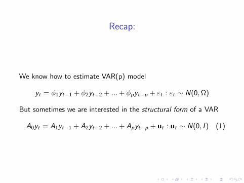
Last time we discussed how to estimate A0 using the Choleskidecomposition
I This implied ordering the variables according tocontemporaneous causality
Whether this is a good idea or not cannot be judged by simplylooking at the data
I Identifying assumptions need to be motivated carefully andappear sensible on an a priori basis
Recap:
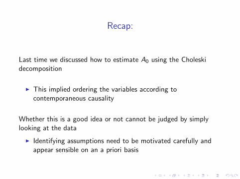
To go from reduced form
yt = φ1yt−1 + φ2yt−2 + ...+ φpyt−p + εt
= A−10 A1yt−1 + A−1
0 A2yt−2 + ...+ A−10 Apyt−p + A−1
0 ut
to the structural form we assumed that A0 is lower triangular
A0yt = A1yt−1 + A2yt−2 + ...+ Apyt−p + ut
so that A−10 =chol(Ω).
I Important: There are (infinitely) many ways to orthogonalizethe reduced form errors εt that all fit the data equally well:
I There exists an infinite number of orthonormal matrices Tsuch that TT ′ = I and hence A−1
0 TT ′(A−1
0
)′= Ω
Long run restrictions
Another class of “weak” restriction that may hold across a largerange of models are so called long run restrictions
I First suggested by Blanchard and Quah (1989)
The idea: There may a be a subset of shocks that havepermanent effects on some variables but not on others, and shocksthat have no permanent effects on any variables
I This splits reduced form shocks into permanent shocks and”everything else”
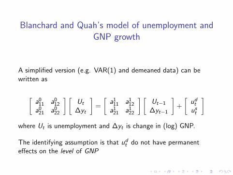
Blanchard and Quah’s model of unemployment andGNP growth
A simplified version (e.g. VAR(1) and demeaned data) can bewritten as
[a0
11 a012
a021 a0
22
] [Ut
∆yt
]=
[a1
11 a112
a121 a1
22
] [Ut−1
∆yt−1
]+
[udtust
]where Ut is unemployment and ∆yt is change in (log) GNP.
The identifying assumption is that udt do not have permanenteffects on the level of GNP
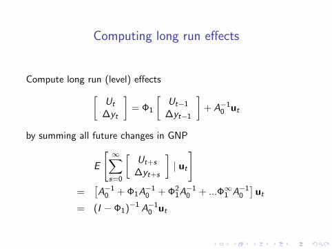
Computing long run effects
Compute long run (level) effects[Ut
∆yt
]= Φ1
[Ut−1
∆yt−1
]+ A−1
0 ut
by summing all future changes in GNP
E
[ ∞∑s=0
[Ut+s
∆yt+s
]| ut
]=
[A−1
0 + Φ1A−10 + Φ2
1A−10 + ...Φ∞1 A−1
0
]ut
= (I − Φ1)−1 A−10 ut
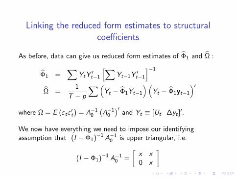
Linking the reduced form estimates to structuralcoefficients
As before, data can give us reduced form estimates of Φ1 and Ω :
Φ1 =∑
YtY′t−1
[∑Yt−1Y
′t−1
]−1
Ω =1
T − p
∑(Yt − Φ1Yt−1
)(Yt − Φ1yt−1
)′where Ω = E (εtε
′t) = A−1
0
(A−1
0
)′and Yt ≡ [Ut ∆yt ]
′.
We now have everything we need to impose our identifyingassumption that (I − Φ1)−1 A−1
0 is upper triangular, i.e.
(I − Φ1)−1 A−10 =
[x x0 x
]
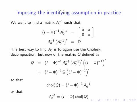
Imposing the identifying assumption in practice
We want to find a matrix A−10 such that
(I − Φ)−1 A−10 =
[x x0 x
]A−1
0
(A−1
0
)′= Ω
The best way to find A0 is to again use the Choleskidecomposition, but now of the matrix Q defined as
Q ≡ (I − Φ)−1 A−10
(A−1
0
)′ ((I − Φ)−1
)′= (I − Φ)−1 Ω
((I − Φ)−1
)′so that
chol(Q) = (I − Φ)−1 A−10
or thatA−1
0 = (I − Φ) chol(Q)
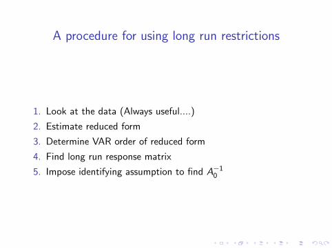
A procedure for using long run restrictions
1. Look at the data (Always useful....)
2. Estimate reduced form
3. Determine VAR order of reduced form
4. Find long run response matrix
5. Impose identifying assumption to find A−10

Step 1: Look at the data
1950 1960 1970 1980 1990 2000 2010-4
-2
0
2
4
6US unemployment
1950 1960 1970 1980 1990 2000 2010-4
-2
0
2
4US GDP growth
Step 2 and 3
Estimate reduced form
I Standard OLS
Determine VAR order of reduced form
I Use LR test or FPE, AIC, HQ or Schwarz criterion
We know how to do all this, but let’s look at plots.

Determine VAR order: LR tests
0 2 4 6 8 10 120
100
200
300
400
500
600
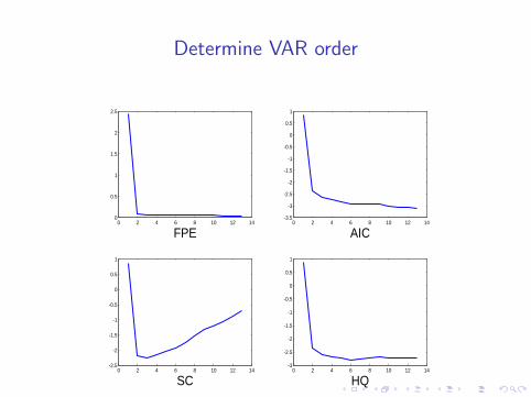
Determine VAR order
0 2 4 6 8 10 12 140
0.5
1
1.5
2
2.5
FPE0 2 4 6 8 10 12 14
-3.5
-3
-2.5
-2
-1.5
-1
-0.5
0
0.5
1
AIC
0 2 4 6 8 10 12 14-2.5
-2
-1.5
-1
-0.5
0
0.5
1
SC0 2 4 6 8 10 12 14
-3
-2.5
-2
-1.5
-1
-0.5
0
0.5
1
HQ
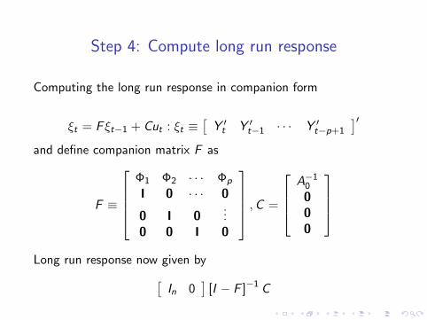
Step 4: Compute long run response
Computing the long run response in companion form
ξt = F ξt−1 + Cut : ξt ≡[Y ′t Y ′t−1 · · · Y ′t−p+1
]′and define companion matrix F as
F ≡
Φ1 Φ2 · · · Φp
I 0 · · · 0
0 I 0...
0 0 I 0
,C =
A−1
0
000
Long run response now given by[
In 0]
[I − F ]−1 C
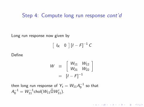
Step 4: Compute long run response cont’d
Long run response now given by[IK 0
][I − F ]−1 C
Define
W ≡[W11 W12
W21 W22
]= [I − F ]−1
then long run response of Yt = W11A−10 so that
A−10 = W−1
11 chol(W11ΩW ′11).
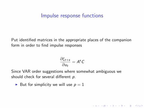
Impulse response functions
Put identified matrices in the appropriate places of the companionform in order to find impulse responses
∂ξt+s
∂ut= AsC
Since VAR order suggestions where somewhat ambiguous weshould check for several different p.
I But for simplicity we will use p = 1
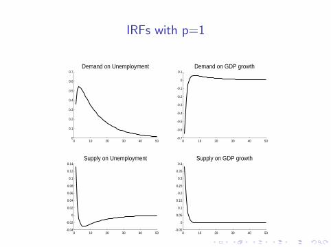
IRFs with p=1
0 10 20 30 40 500
0.1
0.2
0.3
0.4
0.5
0.6
0.7Demand on Unemployment
0 10 20 30 40 50-0.7
-0.6
-0.5
-0.4
-0.3
-0.2
-0.1
0
0.1Demand on GDP growth
0 10 20 30 40 50-0.04
-0.02
0
0.02
0.04
0.06
0.08
0.1
0.12
0.14Supply on Unemployment
0 10 20 30 40 50-0.05
0
0.05
0.1
0.15
0.2
0.25
0.3
0.35
0.4Supply on GDP growth
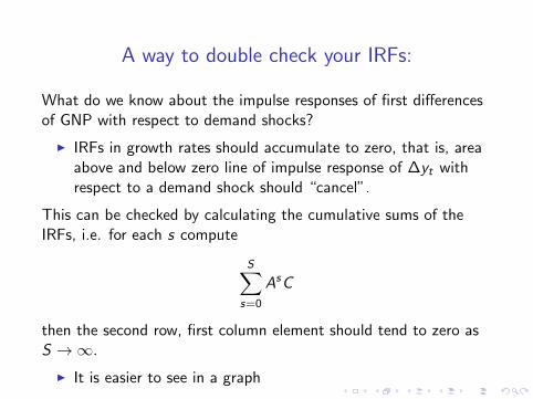
A way to double check your IRFs:
What do we know about the impulse responses of first differencesof GNP with respect to demand shocks?
I IRFs in growth rates should accumulate to zero, that is, areaabove and below zero line of impulse response of ∆yt withrespect to a demand shock should “cancel”.
This can be checked by calculating the cumulative sums of theIRFs, i.e. for each s compute
S∑s=0
AsC
then the second row, first column element should tend to zero asS →∞.
I It is easier to see in a graph
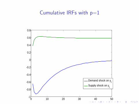
Cumulative IRFs with p=1
0 10 20 30 40 50-1
-0.8
-0.6
-0.4
-0.2
0
0.2
0.4
0.6
0.8
Demand shock on yt
Supply shock on yt

Variance decomposition
1. Start by computing the unconditional variance
Σyy = ΦΣyΦ′ + CC ′ =
[σ2
∆y σ∆yu
σu∆y σ2u
]2. Compute variance of first variable using c1c
′1 instead of CC ′ in
Σy1 = ΦΣy1Φ′ + c1c′1
=
[σ2
∆y1 σ∆yu1
σu∆y1 σ2u1
]3. Divide the resulting diagonal elements with corresponding
diagonal element of unconditional covariance matrix, i.e.
compute the fractionsσ2
∆y1
σ2∆y
andσ2u1σ2u
to get the fraction of the
unconditional variances explained by the first shock.
4. Repeat step 2-3 for each shock
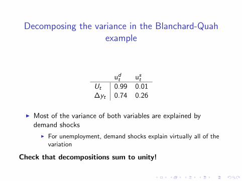
Decomposing the variance in the Blanchard-Quahexample
udt us
t
Ut 0.99 0.01∆yt 0.74 0.26
I Most of the variance of both variables are explained bydemand shocks
I For unemployment, demand shocks explain virtually all of thevariation
Check that decompositions sum to unity!

Historical Decompositions
What shocks at what time contributed to the business cycle duringeach moment in the sample?
Yt = ΦYt−1 + Cut
= ΦtY0 + Φt−1Cu1 + ...+ Φt−sCus + ...+ Φt−t+1Cut−1 + Cut
Decompose into the effect of each shock in period t as
Yt = ΦtY0 + Φt−1c1u1,1 + ...+ Φt−t+1c1u1,t−1 + c1u1,t
+Φt−1c2u2,1 + ...+ Φt−t+1c2u2,t−1 + c2u2,t
We can compute this for each t if we have a time series for the ut
given byut = C−1 (Yt − ΦYt−1)
It is illustrative to plot all this in one graph, containing y1t , y11,t
and y12,t and initial conditions effects.

Historical decomposition
1950 1960 1970 1980 1990 2000 2010-4
-2
0
2
4
6
ud
us
Y0
Unemployment
1950 1960 1970 1980 1990 2000 2010-4
-2
0
2
4
ud
us
Y0
GDP growth
Other examples of long run restrictions
Gali (1999) uses long run restrictions to analyze the implications ofpermanent productivity shocks for employment and hours worked.
I Identifying assumption: Only productivity shocks can havepermanent effects on level of output
I Finds that identified productivity shocks do not cause anincrease in hours worked or employment, as suggested by RBCmodels
I Gali argues that this is evidence in favor of New Keynesianmodels with sticky prices.
I NK models predict that hours fall after productivity shock
More on this after the break....
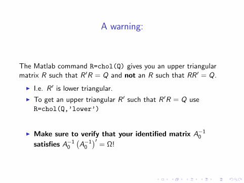
A warning:
The Matlab command R=chol(Q) gives you an upper triangularmatrix R such that R ′R = Q and not an R such that RR ′ = Q.
I I.e. R ′ is lower triangular.
I To get an upper triangular R ′ such that R ′R = Q useR=chol(Q,’lower’)
I Make sure to verify that your identified matrix A−10
satisfies A−10
(A−1
0
)′= Ω!
Two critiques of SVARs
1. Rudebusch vs Sims
2. Minnesota vs Long Run restrictions
Rudebusch vs Sims
Rudebusch (1998) argues that SVAR measures of monetary policydo not make sense
Sims argues that they do
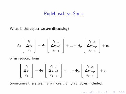
Rudebusch vs Sims
What is the object we are discussing?
A0
rt∆ytπt
= A1
rt−1
∆yt−1
πt−1
+ ...+ Ap
rt−p∆yt−pπt−p
+ ut
or in reduced form rt∆ytπt
= Φ1
rt−1
∆yt−1
πt−1
+ ...+ Φp
rt−p∆yt−pπt−p
+ εt
Sometimes there are many more than 3 variables included.
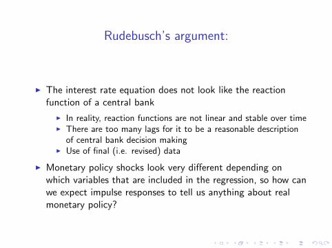
Rudebusch’s argument:
I The interest rate equation does not look like the reactionfunction of a central bank
I In reality, reaction functions are not linear and stable over timeI There are too many lags for it to be a reasonable description
of central bank decision makingI Use of final (i.e. revised) data
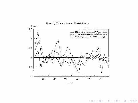
I Monetary policy shocks look very different depending onwhich variables that are included in the regression, so how canwe expect impulse responses to tell us anything about realmonetary policy?
Sims’ counter argument
I Linearity and time invariance are always approximations andthis is a problem common to all macroeconomic models.Non-linearity and time varying rules add little explanatorypower, though.
I Long lags in ”reaction function” is just a statistical summarythat does not imply that the Fed responds to ”oldinformation”.
I Revised data: Can be handled by restricting the response ofinterest rates to only variables that are observed at the timeof the decision.
I Sims has a subtle but important point about the how modelscan disagree about the shocks but agree about the effects ofmonetary policy.
Chari, Kehoe and McGrattan (JME2008)
Some background:
I SVARs using long run restrictions (e.g. Gali 1999) similar toBlanchard and Quah’s (1989) find that hours worked decreasein response to permanent productivity shocks
I This is bad news for RBC models since they imply that hoursshould increase in response to productivity
I Conclusion: Only models fitting this pattern (i.e. sticky pricemodels) are worth pursuing.
Chari et al challenges this conclusion
Chari, Kehoe and McGrattan (JME2008)
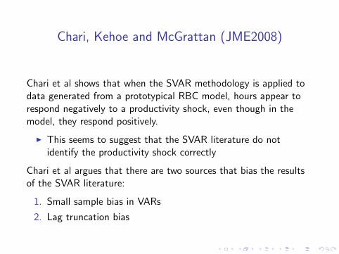
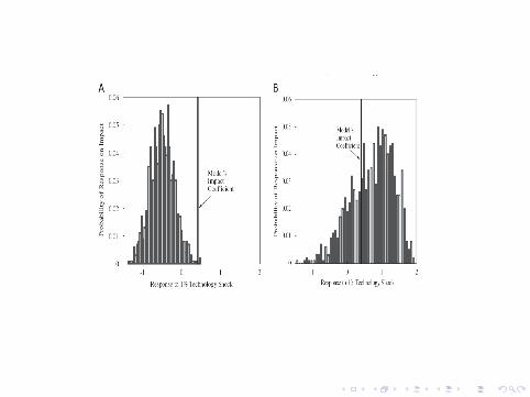
Chari et al shows that when the SVAR methodology is applied todata generated from a prototypical RBC model, hours appear torespond negatively to a productivity shock, even though in themodel, they respond positively.
I This seems to suggest that the SVAR literature do notidentify the productivity shock correctly
Chari et al argues that there are two sources that bias the resultsof the SVAR literature:
1. Small sample bias in VARs
2. Lag truncation bias
Chari, Kehoe and McGrattan (JME2008)
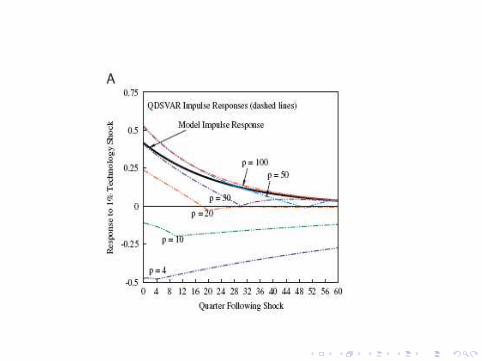
Lag truncation bias:The structural model can be written as an MA(∞)
Yt = A0εt + A1εt−1 + ...+ Asεt−s : s →∞≡ A(L)εt
An implicit assumption in the SVAR literature is that A(L)−1 existsand is equal to I −
∑pi=1 BiL
i so that there exists a finite orderVAR
[I −p∑
i=1
BiLi ]Yt = εt
where p is a low number (typically p = 4).
Suggested strategy to use SVARs to guide modeldesign
I It is risky to compare estimated IRFs to true model IRFs
I A better strategy is to compare estimated IRFs from actualdata with estimated IRFs from data generated by theoreticalmodel
The Minnesota slogan is Do to the model what you do to the dataThat is reasonable advice
I Also applies to de-trending issues etc
Recommended