£So-S-11
STUDl.ES IN RURAL FINANCE
AGRICULTURAL FINANCE PROGRAM ,
Department of Agricultural Economics and Rural Sociology
THE OHIO STATE UNIVERSITY
COLUMBUS, OHIO
43210
Economics and Sociology Occasional Paper # 511
RURAL HOUSEHOLD SAVINGS BEHAVIOR IN SOUTH KOREA, 1962-1976
by
K. N. Hyun D. W Adams
L. J. Hushak
July 24, 1978
••
..
'
RURAL HOUSEHOLD SAVINGS BEHAVIOR IN SOUTH KOREA, 1962-1976*
by
K. N. Hyun, D. W Adams and L. J. Hushak
Savings behavior in high-income countries has drawn
substantial attention from economists the past several
decades. Analysis of aggregate or urban household in-
formation in these countries has led to development of
very useful theories about savings behavior [Mikesell
and Zinser]. Only recently, however, have a small
number of studies been done on rural household savings
in low-income countries [Adams, 1978]. Lack of approp-
riate data has slowed this analysis and made it diffi-
cult for researchers to apply new theories, such as the
permanent income hypothesis, to the analysis of rural
savings behavior. Those interested in this topic have
been forced to use fragmentary, cross-sectional infor-
mation, often collected for some other purpose in order
to shed light on rural savings activities. Because of
these data limitations, researchers also have been
forced to relate savings behavior largely to current
household income. The paucity of research on this topic
has made it nearly impossible to confirm or dispel myths
* The Agency for International Development provided support for this study .
••
-2-
which pervade the development literature about rural
savings behavior: e.g., rural households are too poor
to save, rural households getting more income will
engage in consumption orgies, rural households are not
able to defer gratification by postponing consumption,
and rural households are insensitive to savings incen-
tives and opportunities.
Research on rural savings in low-income countries
is further complicated by the adverse effects of many
government policies on rural household incomes and
low-income countries. These include concessional inter-
est rate policies, product and input prices, taxes, and
foreign exchange regulations which result in low incomes
and weak incentives to save in rural areas. It is im-
possible to answer directly questions about what savings
behavior would have been in a country if policies had
provided more income and stronger savings incentives in
rural areas. Only indirect answers are possible which
are drawn from analysis of rural household savings per
formance in those few countries which have allowed rural
incomes to grow substantially, and have also provided
significant positive incentives and opportunities for
rural households to save.
..
'
-3-
During the past dozen years, South Korea appears to 1/
have provided a positive environment for rural savers.-
South Korea also has assembled rural household data
through representative Farm Household Economy Surveys
since 1962 which are rich enough in detail and also
reliable enough to justify careful analysis of savings
behavior . .2./ A further advantage of this data is that
time series as well as cross-sectional analysis can be
done on individual households. This allows comparison
of savings behavior results from cross-sectional analysis
with time series data.
In the following discussion we attempt to do two
things. The first objective is to document the extent of
voluntary rural household savings in South Korea among
Survey Households from 1962 to 1976. The second objective
is to test a technique recently suggested by several re-
searchers for estimating permanent household income from
cross-sectional data [Bhalla]. If this technique proves
to be reliable, it will allow more comprehensive analysis
of savings behavior in countries where only cross-sectional
data are available.
1/ Another of very few such examples is Taiwan [Ong and others].
2/ See Hyun for more details on these annual surveys carried out by the Ministry of Agriculture and Fisheries.
. -~
-·
•
-4-
Rural Household Incomes and Savings
The Korean economy as well as the agricultural
sector have grown substantially since the early 1960's.
Gross national product has increased by almost 10 percent
per year since 1962 and per capita income in real terms
has gone up nearly six-fold. Growth in the agricul
tural sector has been less spectacular but none the
less impressive, given the very limited land resources
in South Korea. The real value of agricultural output
more than doubled from 1962 to 1976. Major financial
market and foreign exchange reforms in 1965, and adjust
ments in pricing policies in the late 1960's and early
1970's have substantially improved farmers' incomes
and their incentives to save [Brown].
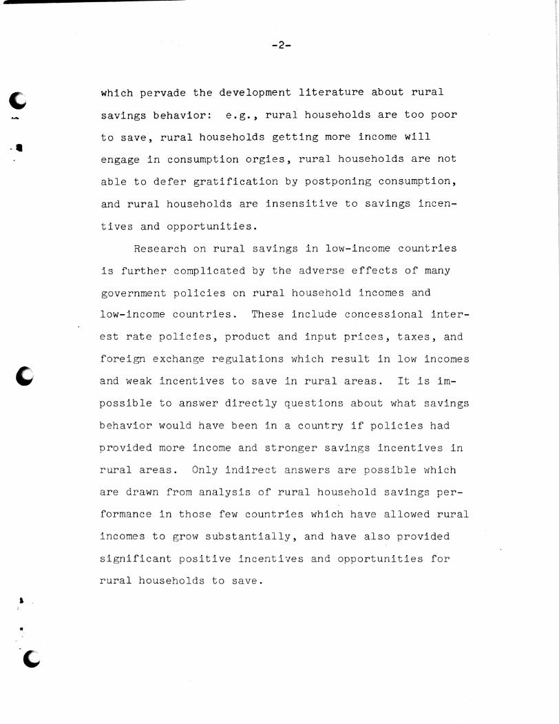
As can be noted in Table 1, average net real income
of the Farm Economy Survey households increased two and
a half times from 1962 to 1976. In comparison with
other more developed countries, however, rural incomes
were still quite low throughout the period. In 1962,
average rural farm household income was less than $600
per year. This only amounted to about $90 per capita.
The substantial increase in income by 1976 raised house
hold incomes to about $1460 and per capita incomes to
about $260. By international standards these rural
households are far from being affluent .
Year
1962 1963 1964 1965 1966
1967 1968 1969 1970 1971
1972 1973 1974 1975 1976
.. · ... TABLE 1: Average Household Income, Consumption Expenditures and Propensity
to Save of Farm Economy Survey Households in Korea, 1962-1976
Net b/
Household-Household Consumption Gross
Households Income Expenditures Savings (1) (2) (3)=(1)-(2)
Number (In 1970 a/
Korean 1,000 Won- )
1,163 177 150 27 1,161 201 177 24 1,172 204 173 31 1,173 166 157 9 1,180 177 157 20
1,176 190 170 20 1,181 212 176 36 1,180 241 197 44 1,180 259 218 41 1,180 333 235 98
1,182 352 263 89 1,170 369 270 99 2,515 366 242 124 2,517 373 271 102 2,516 444 298 146
.. .
Average Propensity
to Save (4)=(3)/(1)
.15
.12
.15
.05
.12
.11
. 17
.18
.16
.29
.25
.27
.34
.27
.33
SOURCE: Ministry of Agriculture and Fisheries (MAF), Republic of Korea, Report on the Results of Farm Household Economy Survey, yearly reports from 1962 to 1976 (Seoul, Korea; MAF, various years 1963 through 1977).
~/Adjusted to 1970 prices using Index of Wholesale Prices of Korea. In 1970t the average exchange rate of won for a U.S. dollar was 304.
~/Includes household payments for taxes and interest.
I V1 I
•
-6-
Although not shown in Table 1, about 20 percent
of household income was provided by off-farm earnings
throughout the period. Changes in weather and govern
ment pricing policies were important factors explain
ing major changes in incomes in the mid-1960's, the
late 1960 1 s, and early 1970's. As might be expected,
household consumption expanded with household incomes,
but at a slower rate. This resulted in sharp increases
in household gross savings, especially after the mid-
1960's. The average propensity to save jumped from
only .15 in 1962 to .33 in 1976. Despite relatively
low absolute levels of income, rural households in
South Korea have saved very large proportions of their
incomes the past few years.
Without complicated analysis, one can conclude
that a major part of this increase in expressed savings
resulted from the expansion in real household incomes.
As Wai has pointed out, however, incentives and oppor
tunities to save are important factors which help explain
part of savings behavior. Friedman and others have
argued that the quality of household income flows also
may help to explain this behavior. Quality may be
indicated by the stability of the flow or by measures
of permanent and transitory components of the flows.
Still other researchers argue that changing characteristics
of the household itself may influence consumption-savings
behavior.
-7-
The household data used in this study do not in-
elude information which sheds much light on savings
opportunities or incentives.l/ The data do allow
analysis of the effects on savings behavior of per-
manent income, and various household characteristics.
Major emphasis will be placed in the following discus-
sion on measuring the influence of permanent and tran-
sitory income.
Empirical Models
Friedman's permanent income hypothesis rests on several
main tenets [Friedman, p. 222]. These include that a con
sumer's measured (observed) income (Y) and consumption (C)
in a particular period may be separated into transitory
and permanent income (Yp). That is, marginal and average
propensities to consume out of permanent income are in-
dependent of the level of permanent income. Also, that
transitory and permanent components are uncorrelated.
A number of empirical tests of this hypothesis have shown
that the marginal propensity to consume (MPC) out of trans-
itory income is greater than zero, but less than MPC out
of permanent income [Ferber].
}/ Lee and others have argued that improved access to financial savings facilitates in agricultural cooperatives over the 1961-75 period was an important stimulant to voluntary rural savings in South Korea.
'I ...
-8-
Friedman has proposed that permanent consumption be
assumed equal to measured consumption (C). Statistically,
the permanent income hypothesis can be stated as,
(1) C = b1Y + b2Yp + e
where b1 is the MPC out of transitory income, (b1 + b2)
is the MPC out of permanent income, and e is the random
error.
Studies in low-income countries suggest that other
household characteristics and returns to investments also
affect consumption-savings behavior.ii Under the per- ·
manent income hypothesis it is argued that additional
variables affect the MPC out of permanent income (b2).
Assuming the relationship is linear,
(2) b2 = b20 + b21LD + b22SI + b23RT + b24LQ
+ b 25DP
Substitution into the consumption function (1) gives
(3) C = b1Y + b20Yp + b 21LD Yp + b22SI Yp
+ b23RT Yp + b24LQ Yp + b25DP Yp + e,
where LD is hectares of cultivated land area, SI reflects
source of incomes which is defined as the ratio of gross
farm income to gross household income, RT is the rate of
return to capital during the previous year, LQ is the value
of liquid assets, and DP is the ratio of dependents to
ii Two comprehensive reviews of the consumption-savings literature in low-income countries are Snyder and Alamgir.
'
-9-
total family members.21 Following Girao and others,
equation (2) is assumed to be nonstochastic.
Farm size (LD) is used as a proxy for farm invest-
ment opportunities. The coefficient b 21 is expected to
be negative [Kelly and Williamson]. The source of in-
come ratio (SI) indirectly influences consumer behavior
through investment opportunities, relative stabilities of
various income flows, prices of industrial goods, and de-
monstration effects of urban consumption patterns [Adams
and others, 1975]. If farmers have relatively unstable
farm incomes the coefficient b 22 is expected to be negative.
The rate-of-return to capital (RT) is used as a
proxy for the profitability of all household investments.
This variable also serves as the opportunity cost of
current consumption versus future consumption. Theore-
tically, farmers who have high expected rates-of-return
on capital will increase their investment in farm capital
and also switch more of their current income to savings
[Adams and others, 1975]. The relationship between the re
turn to capital and MPC (b23) depends on the source of
the investment funds. If funds come from reduced con-
sumption, the expected sign is negative. On the other
hand, if funds come from increased borrowings or liqui-
dating other assets to make investments, a positive
relationships is expected.
.2/ Detailed definitions of the variables used in the analysis are presented in the Appendix.
'
-10-
The value of liquid asset holdings (LQ) is a rough
measure of wealth. Several empirical studies have sug
gested that liquid assets are important factors affect
ing savings behavior [for example, Mizoguchi]. The
coefficient b 24 is expected to be positive. The depend
ency ratio (DP) is a measure of the proportion of house
hold members who do not contribute to household income.
The coefficient b 25 is expected to be positive because
a higher DP increases consumption without changing
income [Leff].
As an alternative against which to compare results
of the permanent income consumption function (3), a
Keynesian consumption function is estimated. It is of
the general form
(4) c = a 0 + a 1Y + E a 0 jzj + E a 1 jzj Y + e,
where Z refers to the set of the other variables expected
to affect consumption behavior.
Measurement of Permanent Income
From an empirical point of view, the permanent in
come hypothesis is difficult to test because of the
problem of measuring a consuming unit's permanent in
come. As mentioned earlier, due to the lack of data
this difficulty is serious in low-income countries.
Some empirical studies in low-income countries have used
moving averages of the previous two or three year's
' . .
-11-
incomes, or cell means of income for grouped families
as proxies for permanent income [Snyder] .
In this study, two different measures of permanent
income are used: predicted income from an income esti-
mating function and a weighted average of past observed
incomes. Bhalla recently used an "earnings function"
to estimate the impact which permanent household
characteristics have on the earnings of rural households
in India. His analysis builds on earlier earnings func-
tion work by Gordon, Lillard and others. Following
Bhalla, it is hypothesized that various permanent house-
hold characteristics, which have been used for tests of
the permanent income hypothesis, explain permanent in-
come through a functional relationship. Under this
hypothesis, permanent income can be estimated with the
statistical model
(5) Y = c 0 + c 1LD + c 2LQ + c 3ED + c4FM + c 5DP
+ c6SI + u
where ED is average years of schooling of household
members more than six years of age, FM is family size,
and other variables are as defined previously. The
predicted values of income (Y) are the values of perma
nent income for each household, and the residuals (u)
are the values of transitory income.
'
-12-
The advantage of this technique is that it can
be estimated from cross-sectional data for a single
year. The disadvantage is that it cannot account for
cyclical changes which cause the total sample to de
viate uniformly from expected income. However, if the
explanatory variables in equation (5) measure the hu
man and physical resources of households, the predicted
incomes will at least reflect the relative permanent
income status of households in the sample and can be
used as measures of permanent income in consumption
function estimation.
The second method of measuring permanent income is
a weighted average of measured incomes for the most re
cent three years, including the year considered. As
Friedman suggested, permanent income is usually measured
by a weighted average of current and past values of
measured incomes with weights declining exponentially.
This method, however, requires fairly long time-series
data. With only three years of income data available
to us for this study, the weights were arbitrarily desig
nated, and permanent incomes calculated as follows:
(6) Yp = .5Y + .3Y_1 + .2Y_2,
where subscripts are numbers for lagged years.
'
'
-13-
Results of Model Estimation
The data used in the analysis come from panel house-
holds in the Korean Farm Household Economy Survey. There
were 131 households which were surveyed each year 1968
through 1970. Analysis of this panel data for 1970 make
up the main body of this section. The data for 1968
and 1969 are used only for calculating permanent income
as specified by equation (6), the second measure of per-
manent income, and the rate-of-return on capital in the
previous year.
The estimate of equation (5) from which household
permanent income estimates are obtained is
A Y = Yp(l) = 140.59 + 137.92LD + 0.146LQ + 16.llFM
(32.77) (15.58) (0.39 (4.03)
2 68.llDP - 143.06SI, R = 0.627; F = 42.07; (36.52) (38.44)
where standard errors are in parentheses. The schooling
variable (ED) was dropped; it had a negative coefficient
which was not significantly different from zero. Summary
statistics of the permanent (Yp) and transitory (Ytr) in
come estimates from statistical estimation of equation (5)
and the weighted averages defined by equation (6) are
presented in Table 2. The two measures of permanent in-
come have similar standard deviations and a simnle car-
relation of 0.945, indicating that they are providing
~
'
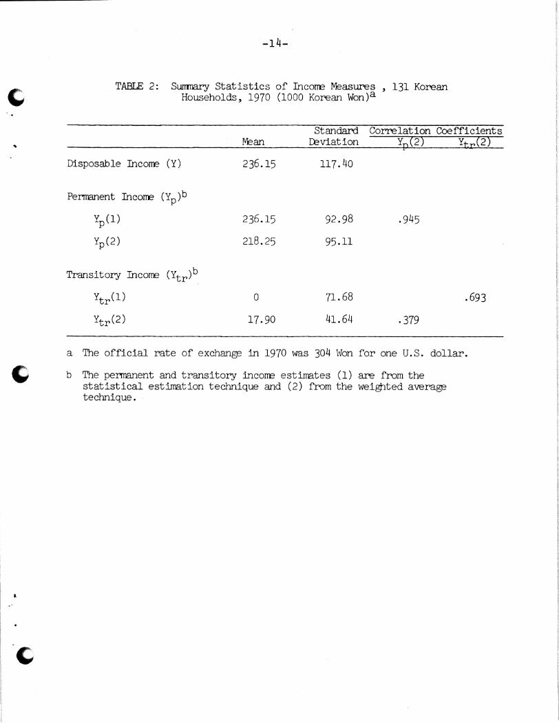
TABI.E 2: Surrrnary Statistics of Incorre Measures , 131 Korean Households, 1970 (1000 Korean Won)a
Standard Correlation Coefficients IVE an Leviation Yp(2) YtrC2)
Disposable Incorre (Y) 236.15 117.40
Permanent Income (Y )b p
Yp(l) 236.15 92.98 .945
Yp(2) 218.25 95.11
Transitory Income (Ytr)b
Ytr(l) 0 71.68 .693
YtrC2) 17.90 41.64 . 379
a The official rate of exchang,B in 1970 was 304 Won for one U.S. dollar.
b The permanent and transitory incorre estirrates (1) are from the statistical estirration technique and (2) from the weigtited averag,B technique.
I l l I j
J I i
t I I
I
" .
-15-
similar measures of the permanent income status of
sample households. In the consumption function esti
mates, Yp(2) for each household is adjusted upward
by adding mean transitory income (17.9 thousand Won)
to adjust for trend. This has the effect of increas-
ing estimates of MPC out of permanent income because
the consumption function is forced through the origin.
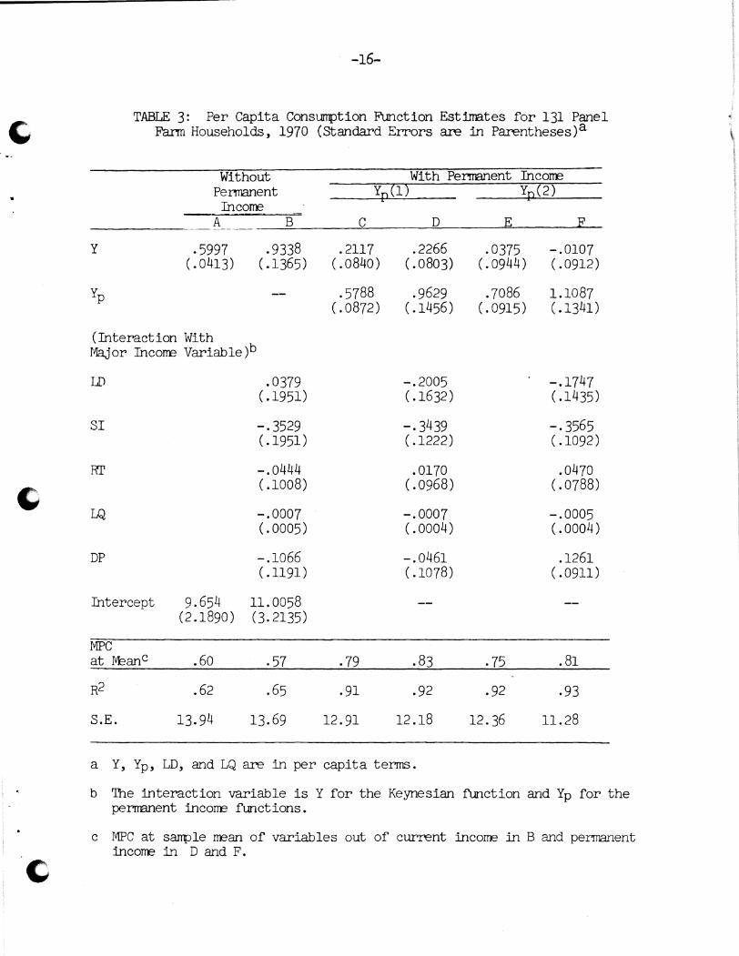
Consumption function estimates are presented in
Table 3 and 4. The estimates in Table 3 are per capita
functions while those in Table 4 are per household.
All equations are statistically significant at the one
percent level.
In Table 3, model A shows that the MPC out of per
manent income is about 0.79, the sum of the coefficients
of the two income variables. Since the coefficient of
Yp(l) is statistically significant at the one percent
level and the sum of the two coefficients is less than
one, the result supports the permanent income hypothesis
that MPC out of permanent income is greater than MPC out
of transitory income, but less than one. The MPC out
of transitory income is about 0.21, which is significantly
greater than zero at the one oercent level. This is con
sistent with empirical findings in other countries that
MPC out of transitory income is greater than zero.
I
-16-
I TABLE 3: Per Capita Consi.mption Function Estirrates for 131 Panel i
~ Farm Households, 1970 (Standard ErTOrs are in Parentheses)a
Without With Pernanent IncoITE .. Permanent Yp(l) Yp(2)
IncoITE A B c D E F -------
y .5997 .9338 .2117 .2266 .0375 -.0107 (.0413) (.1365) (. 0840) (. 0803) (.0944) (.0912)
Yp .5788 .9629 .7086 1.1087 (.0872) (.1456) (. 0915) ( .1341)
(Interaction With Major IncoITE Variable )b
w .0379 -.2005 -.1747 ( .1951) (.1632) ( .1435)
SI -.3529 -. 3439 -. 3565 ( .1951) (.1222) ( .1092)
RI' -.0444 .0170 .0470 ( .1008) (.0968) (. 0788)
LQ -.0007 -.0007 -.0005 (. 0005) (.0004) (.0004)
DP -.1066 -.0461 .1261 ( .1191) ( .1078) (.0911)
Intercept 9.654 11.0058 (2.1890) (3. 2135)
MPC at M?anc .60 .57 . 79 .83 .75 . 81
R2 .62 .65 .91 .92 .92 .93
S.E. 13.94 13.69 12.91 12.18 12.36 11.28
a Y, Yp, LD, and LQ are in per capita terms.
b The interaction variable is Y for the Keynesian function and Yp for the pernanent incorJE functions.
c MPC at sanple ITEan of variables out of current incorre in B and permanent incoITE in D and F.
~
-17-
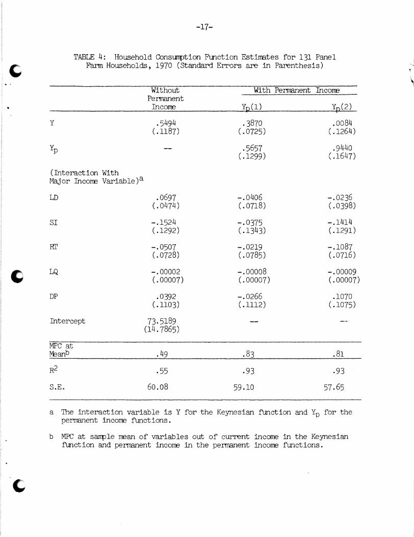
TABLE 4: Household Consumption F'unction Estirrates for 131 Panel
' Farm Households, 1970 (Standard Errors are in Parenthesis)
\ l
Without With Permment Incorre Permment
> .. Income y (1) y (2)
y .5494 . 3870 .0084 ( .1187) (. 0725) ( .1264)
Yp .5657 .9440 (.1299) ( .1647)
(Interaction With Major Income Variable )a
LD .0697 -.0406 -.0236 (.0474) (. 0718) (.0398)
SI -.1524 -.0375 -.1414 (.1292) (.1343) (.1291)
-.0507 -.0219 -.1087 (. 0728) (.0785) (.0716)
~ LQ -.00002 -.00008 -.00009
(.00007) (.00007) (.00007)
DP .0392 -.0266 .1070 (.1103) (.1112) ( .1075)
Intercept 73.5189 (14.7865)
MPC at M2anb .49 .83 .81
R2 .55 .93 .93
S.E. 60.08 59.10 57.65
a The interaction variable is Y for the Keynesian £'unction and Y0 for the perrmnent income functions. -
b MPC at sanple mean of variables out of current income in the Keynesian £'unction and permment income in the permment income functions.
'
-18-
The estimated MPC out of permanent income from the
model Eis about 0.75, which is very close to that esti
mated from model C. The MPC out of transitory income
is essentially zero, supporting Friedman. Overall, it
can be concluded from both consumption function estimates
that MPC out of permanent income is around three quarters,
and is much greater than the MPC out of transitory in
come. In comparison, the simple Keynesian model A shows
that the MPC out of current income is about 0.60. The
standard error of the regression (S.E.) is higher for
model A than for models C and E. This comparison sug
gests that in the consumption models used here, permanent
income variables provide better estimates of consumption
savings behavior than the simple Keynesian formulation.
In models B, D, and F of Table 3, the additional vari
ables expected to affect consumption behavior are added.
In Table 4 estimates of the same consumption functions are
presented using per household variables instead of per capita
variables. The Keynesian estimates exclude the shift vari
ables (Ea0 jZj in equation 4); when both shift and inter
action variables are included the MPC is small, e.g., 0.28
at the sample mean in the per capita equation. The esti
mated MPC out of permanent income at the sample mean of
all variables is about 0.83 for Yp(l) and 0.81 for YP(2)
in both the per capita and household consumption functions.
•
'
-19-
functions. These estimates are within one standard error
of the simple consumption function MPC estimates in models
C and E. The MPC out of current income from the Keynesian
functions are 0.57 from model B in Table 3, and 0.49 in
Table 4.
The results of the additional variables are mixed.
Farm size (LD) has the expected negative relationship
with MPC in all permanent income equations, but is not
statistically significant in any equation. The income
source ratio (SI) has the expected negative coefficients
in all equations. It is highly significant in the per
capita equations of Table 3, but not significant in the
household equations of Table 4. The larger magnitude
of the coefficients of LD and SI in the per capita equa
tions than in the household equations presents a puzzle.
There may be an interaction effect among LD, SI, and
family size, but an examination of correlation coeffi
cients and alternative equation estimates did not reveal
a solution. In one alternative, where Y and Yp are per
capita, but LD, SI, and LQ are per household, the coef
ficients of LD and SI are similar to those in the house
hold functions.
The coefficients of RT, LQ, and DP are not statisti
cally significant. The coefficients of RT (rate of return
•
-20-
to capital), which did not have the expected sign, are
mixed. More detailed information on returns to current
investments may have yielded different results. The
coefficients of LQ (liquid assets) are negative in all
equations, while the expected sign was positive. The
dependency ratio (DP), which had an expected positive
relationship with MPC, has coefficients of both signs.
Conclusions
At least two interesting findings emerge from this
study. The first is that farm households in South Korea
have saved voluntarily a remarkably large part of their
incomes since the early 1960s. During the late 1960s
these households saved, on the margin, about one-fifth
of their permanent incomes and about four-fifths of their
transitory incomes. The second finding is that useful
measures of permanent and transitory incomes can be esti
mated from cross-sectional data, and that these estimates
can be helpful in better understanding savings behavior.
Much of the development literature assumes that
significant amounts of voluntary savings will not emerge
from low-income households. Unfortunately, the data used
in this study were not rich enough in detail to allow us
to shed much light on why this assumption appears not to
hold for South Korea. We can only conjecture on reasons
for the relatively high marginal propensities to save
-·
-21-
out of permanent income. At least three possible
explanations merit further analysis. The first
might be related to unique cultural traits. Some ob-
servers have argued that the surprisingly high savings
propensities among rural households in Japan, Taiwan
and South Korea are the result of parsimonious cultural
traits unique to some oriental societies. If this is
true, there is very little for other countries to learn
from the South Korean savings experience. Scattered
reports of substantial voluntary savings by rural house-
holds in some places in India, Latin America, and Africa
cast serious doubt in our minds about the strength of
this argument.
A second explanation might relate to the lack of
reliable data on rural household savings behavior in
most low-income countries. It may be that substantial
unrecorded voluntary savings is taking place in rural
areas of other low-income countries. Most rural house-
hold savings do not move through formal markets where
they can be measured with secondary data. Also, as men-
tioned earlier, rural household income, consumption,
asset and savings activity information is difficult
and costly to collect. Most rural surveys in low
income countries do not include sufficient reliable
and detailed information to document actual savings
-22-
behavior. The remarkable savings performance in
Japan, Taiwan and Korea may reflect better measures
of household savings, rather than unique cultural
traits.
A third explanation might focus on differences
in opportunities and incentives to save. Clearly, the
ability to save, as reflected by level of absolute in
come, is important in explaining savings behavior. We
agree with Wai, however, that providing households
with strong positive incentives to save, plus offering
them additional convenient forms in which to hold their
savings can also stimulate savings. While difficult
to prove statistically with the data available, it ap
pears that South Korea was very effective in providing
savings incentives and opportunities. Policies which
gave these incentives and opportunities to save ought
to be largely transferable to other low-income countries.
The results of our analysis lead us to be optimis
tic about the possiblities of mobilizing voluntary sav
ings in rural areas of low-income countries. Policy
makers might be pleasantly surprised by the results of
well designed rural savings mobilization programs, es
pecially in those times and places where rural household
incomes are growing substantially. Spurts in income may
result in household incomes with significant transitory
•
'
-25-
Liquid Asset Holdings (LQ): the values of product inven
tories, small animals, and cash and quasi-cash hold
ings such as deposits and money lent at the beginning
of the year (1000 Won).
Dependency Ratio (DP): the ratio of family members less
than 15 or over 60 years of age to total family
members.
Family Size (FM): the total number of individuals who
resided in the household during most of the calendar
year.
Education (ED): the average years of schooling of house
hold members more than six years of age.
' ..
-23-
components which are highly susceptible to saving op
portunities and incentives.
•
•
-24-
APPENDIX
Definitions of Terms
Consumption (C): all household expenditures not directly
related to production activities during the calendar
year. It includes an imputed value for in-kind con
sumption, and also purchases of consumer durables
(1000 Won).
Disposable Income (Y): the sum of net farm income and
net non-farm income less tax and interest payments
realized by the household during the year. Farm
income does not include an adjustment for capital
depreciation, but does include an estimated value
of in-kind household consumption and inventory
changes in products (1000 Won).
Farm Size (LD): the total hectares of cultivated land
included in the farm enterprise. Most of this land
is owner-operated.
Source of Income Ratio (SI): the ratio of gross farm in
come to total gross household income.
Rate-of-Return to Capital (RT): the ratio of gross house
hold income to total assets of the previous year.
Ratios for the previous year are used since investment
deicisions are likely heavily influenced by recent
returns to investment .
•
•
•
-26-
References
Adams, Dale W, "Mobilizing Household Savings Through Rural
Financial Markets," Economic Development and Cultural
Change, Vol. 26, No. 3, April 1978, pp. 547-560.
Adams, Dale W and others, "Changes in Rural Purchasing
Power in Taiwan, 1952-72," Food Research Institute
Studies, Vol. 14, No. 2, 1975, pp. 127-145.
Alamgir, Mohiuddin, "Rural Savings and Investment in Devel
oping Countries: Some Conceptual and Empirical Issues,"
The Bangladesh Development Studies, Vol. 4, No. 1,
January 1976, pp. 1-48.
Bhalla, Surjit S., "Aspects of Savings Behavior in Rural
India," Studies in Domestic Finance, No. 31, Public
and Private Finance Division, Development Economics
Department, World Bank, December 1976.
Brown, Gilbert, Korean Pricing Policies and Economic
Development in the 1960's (Baltimore: Johns Hopkins
University Press, 1973).
Canh, Troung Quang, "Income Instability and Consumption
Behavior: A Study of Taiwanese Farm Households
1964-1970," unpublished Ph.D. dissertation, The Ohio
State University, 1974.
Ferber, Robert, "General Theories of Spending or Savings
Behavior," in Sapiro (ed.), Macroeconomics, Selected
Readings (Harcourt, Brace & World, Inc., 1970) .
•
-27-
Friedman, Milton, A Theory of the Consumption Function
(Princeton: Princeton University Press, 1957).
Girao, J. A. and others, "Effect of Income Instability on
farmers Consumption and Investment Behavior: An
Econometric Analysis," Search, Vol. 3, No. l,·Cornell
University of Agricultural Experiment Station, 1973.
Gordon, Roger H., "Essays on the Causes and Equitable
Treatment of Differences in Earnings and Ability,"
unpublished Ph.D. dissertation, Department of Economics,
Massachusetts Institute of Technology, June 1976.
Hyun, Kong-Nam, "Aspects of Rural.Household Saving Behavior
in Korea, 1962-1974," unpublished M.S. thesis, The
Ohio State University, 1977.
Kelly, A. C. and Jeffery G. Williamson, "Household Savings
Behavior in the Developing Economies: The Indonesian
Case," Economic Development and Cultural Change,
Vol. 16, No. 3, April 1968, pp. 385-403.
Lee, Tae Young, Dong Hi Kim and Dale W Adams, "Savings De
posits and Credit Activities in South Korean Agricul
tural Cooperatives 1961-1975," Asian Survey, Vol. 17,
No. 12, December 1977, pp. 1182-1194.
Leff, Nathaniel H., "Dependency Rate and Savings Rates,"
American Economic Review, Vol. 59, No. 5, 1969,
pp. 886-896 .
/ I
c
'
•
-28-
Lilliard, Lee A., "Inequality: Earnings vs. Human Wealth,"
American Economic Review, Vol. 67, No. 2, March 1977,
pp. 42-53.
Mikesell, Raymond F. and James E. Zinser, "The Nature of
the Savings Function in Developing Countries: A
Survey of the Theoretical and Empirical Literature,"
Journal of Economic Literature, Vol. 11, No. 1,
March 1973, pp. 1-26.
Ministry of Agriculture and Fisheries (MAF), Republic of
Korea, Report on the Results of Farm Household Economy
Survey, yearly reports 1962 to 1976 (Seoul, Korea: MAF,
various years 1963 through 1977).
Mizoguchi, Toshiyuki, Personal Savings and Consumption in
Postwar Japan (Tokyo: Kinokuniya Bookstore Co., 1970).
Ong, Marcia M. L. and others, "Voluntary Rural Savings
Capacities in Taiwan, 1960-70," American Journal of
Agricultural Economics, Vol. 58, No. 3, August 1976,
pp. 578-582.
Snyder, Donald W., "Econometric Studies of Household Sav
ings Behavior in Developing Countries: A Survey,"
The Journal of Development Studies, Vol. X, No. 2,
January 1974, pp. 139-153.
Wai, U Tun, Financial Intermediaries and National Savings in
Developing Countries (New York: Praeger, 1972) .
Recommended