ICML07 Tutorial
Amnon Shashua
School of Computer Science & Eng.The Hebrew University
Tensor Methods for Machine Learning, Computer Vision, and Computer
Graphics
Part I:Factorizations and Statistical Modeling/Inference

ICML07 Tutorial
Factorizations of Multi-Dimensional ArraysNormally: factorize the data into a lower dimensional space in order to describe the original data in a concise manner.
Focus of Lecture:
Factorization of symmetric forms Probabilistic clustering.
Factorization of empirical joint distribution Latent Class Model
Factorization of partially-symmetric forms Latent clustering

ICML07 Tutorial
N-way array decompositions
A rank=1 tensor (n-way array) is represented by an outer-productof n vectors
A rank=1 matrix G is represented by an outer-product of two vectors:
ICML07 Tutorial
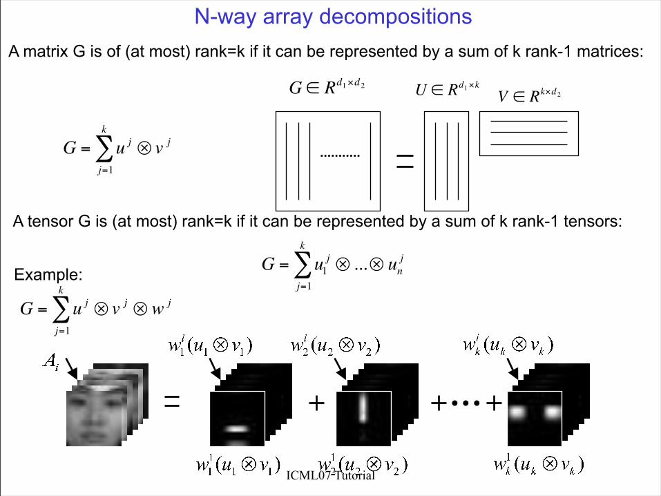
N-way array decompositions A matrix G is of (at most) rank=k if it can be represented by a sum of k rank-1 matrices:
A tensor G is (at most) rank=k if it can be represented by a sum of k rank-1 tensors:
Example:

ICML07 Tutorial
N-way array Symmetric Decompositions
A super-symmetric rank=1 tensor (n-way array) , is represented by an outer-product of n copies of a single vector
A symmetric rank=1 matrix G:
A symmetric rank=k matrix G:
A super-symmetric tensor described as sum of k super-symmetric rank=1 tensors:
is (at most) rank=k.
ICML07 Tutorial 6
General Tensors
Latent Class Models
Hebrew University
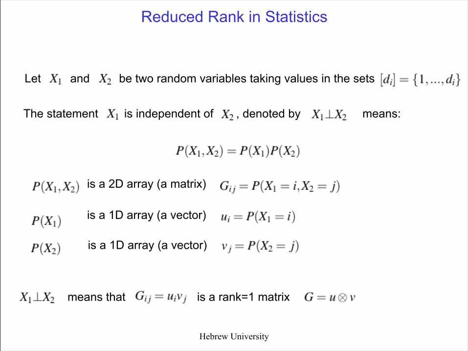
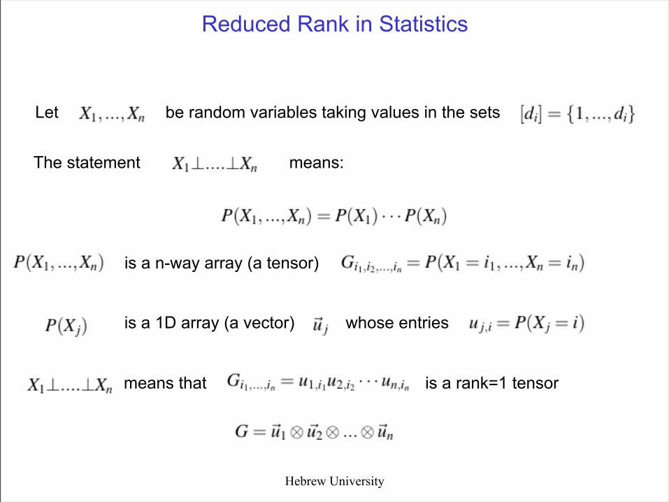
The statement is independent of , denoted by means:
Let and be two random variables taking values in the sets
Reduced Rank in Statistics
is a 2D array (a matrix)
is a 1D array (a vector)
is a 1D array (a vector)
means that is a rank=1 matrix
Hebrew University
The statement means:
Let be random variables taking values in the sets
Reduced Rank in Statistics
is a n-way array (a tensor)
is a 1D array (a vector) whose entries
means that is a rank=1 tensor
Hebrew University
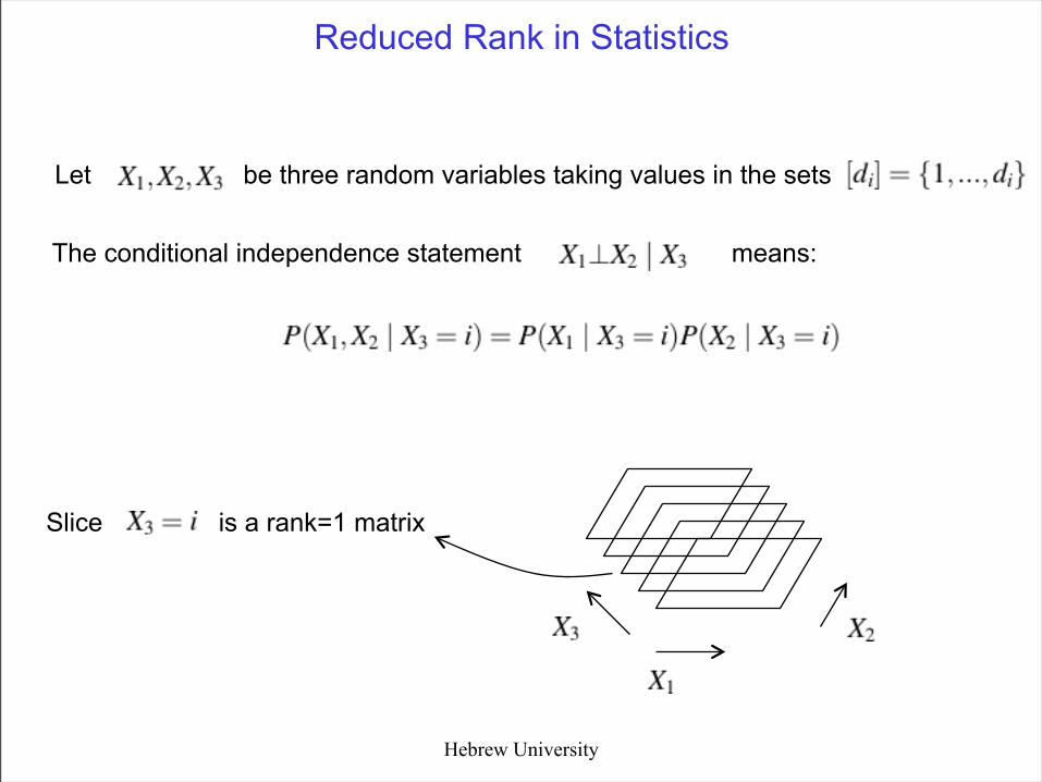
Slice is a rank=1 matrix
The conditional independence statement means:
Let be three random variables taking values in the sets
Reduced Rank in Statistics
Hebrew University
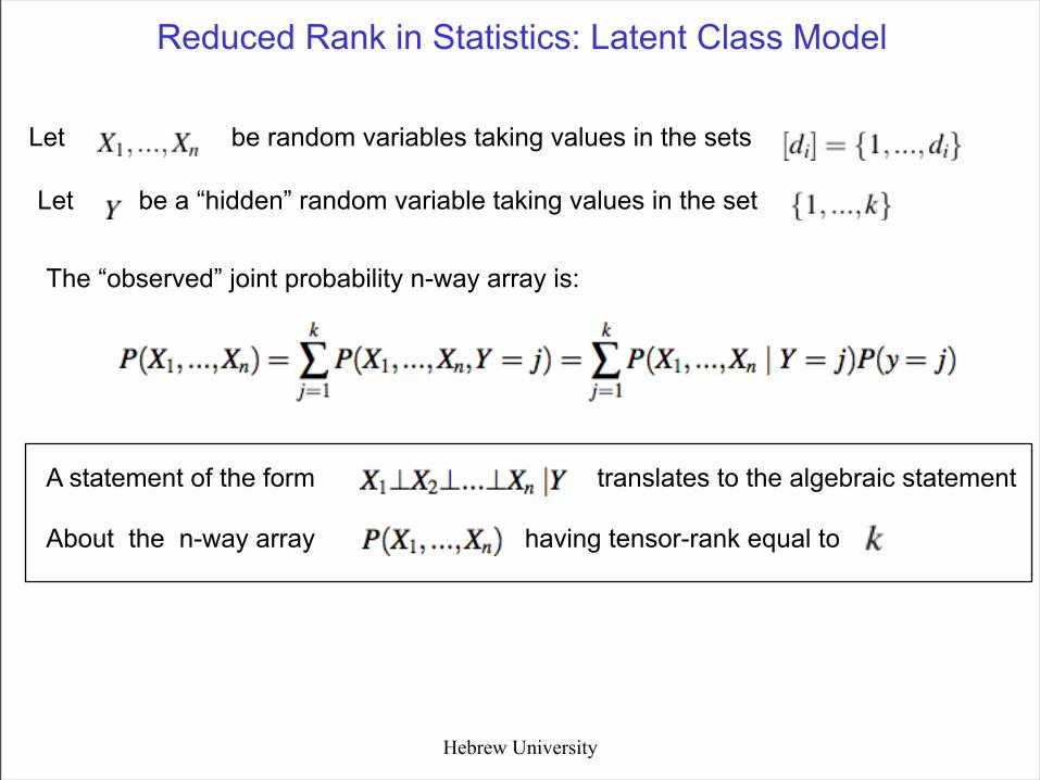
Let be random variables taking values in the sets
Reduced Rank in Statistics: Latent Class Model
Let be a “hidden” random variable taking values in the set
The “observed” joint probability n-way array is:
A statement of the form translates to the algebraic statement
About the n-way array having tensor-rank equal to
Hebrew University
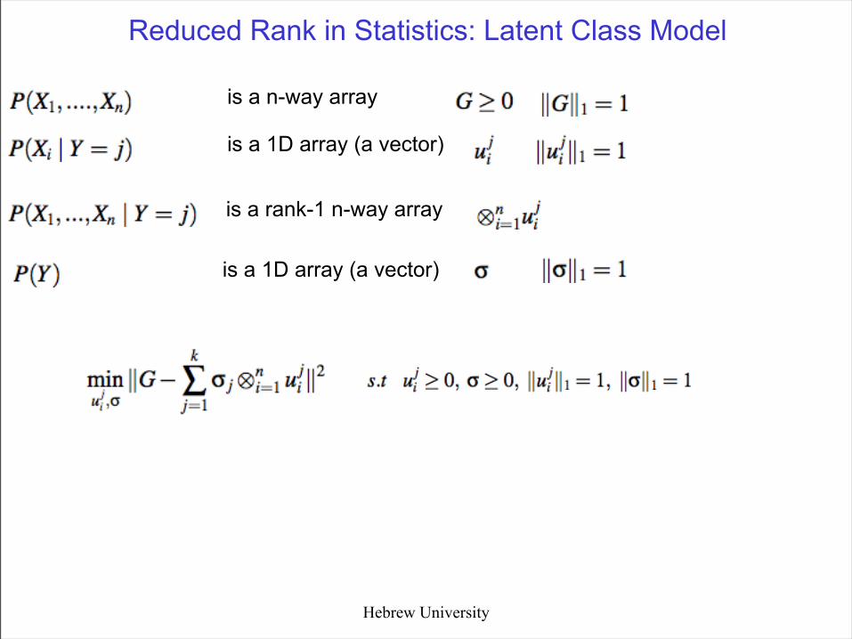
is a 1D array (a vector)
is a rank-1 n-way array
is a 1D array (a vector)
is a n-way array
Reduced Rank in Statistics: Latent Class Model

Hebrew University
Reduced Rank in Statistics: Latent Class Model
for n=2:
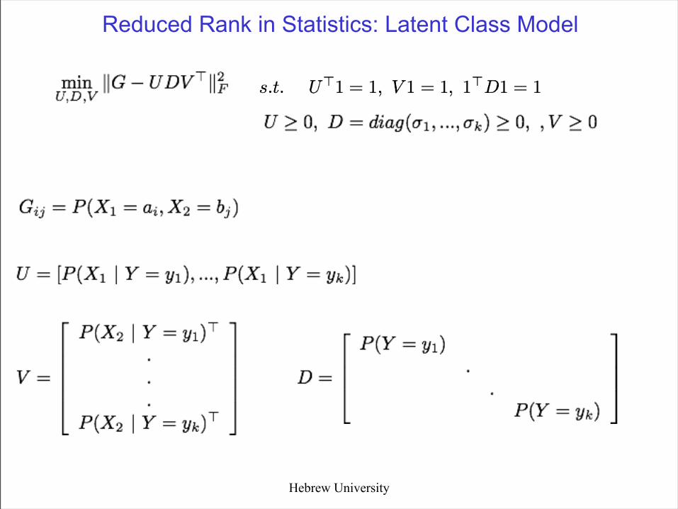
Hebrew University
Reduced Rank in Statistics: Latent Class Model

Hebrew University
Reduced Rank in Statistics: Latent Class Model
when loss() is the relative-entropy:
then the factorization above is called pLSA (Hofmann 1999)
Typical Algorithm: Expectation Maximization (EM)
Hebrew University 15
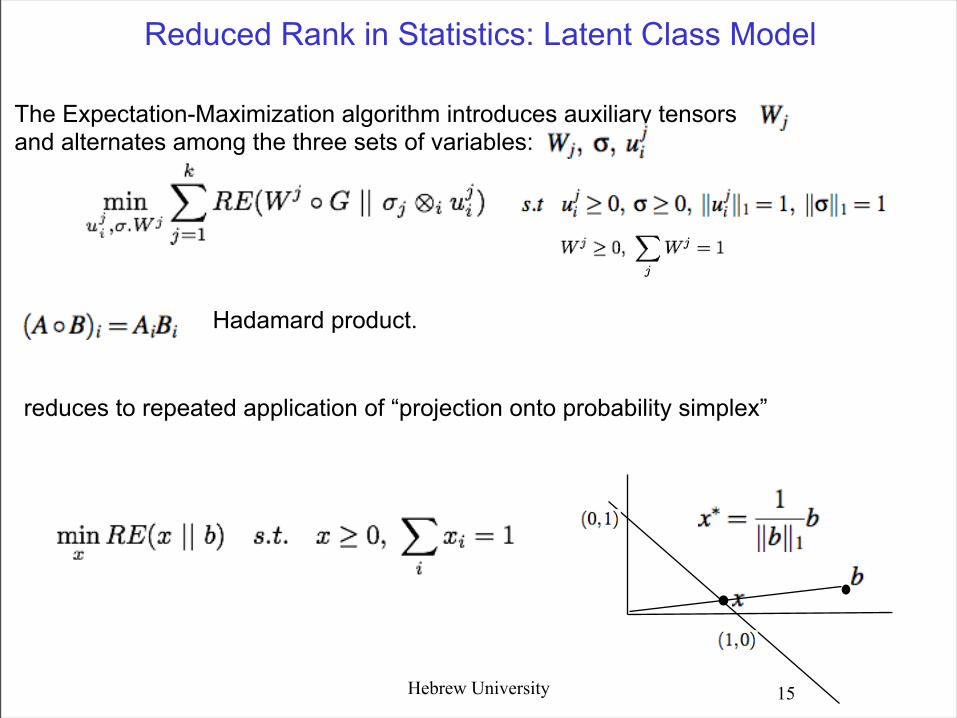
The Expectation-Maximization algorithm introduces auxiliary tensors and alternates among the three sets of variables:
Hadamard product.
reduces to repeated application of “projection onto probability simplex”
Reduced Rank in Statistics: Latent Class Model
Hebrew University
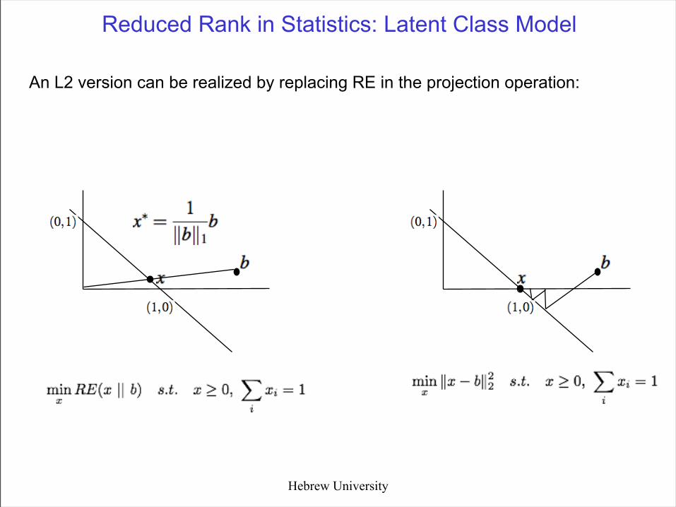
An L2 version can be realized by replacing RE in the projection operation:
Reduced Rank in Statistics: Latent Class Model
Hebrew University
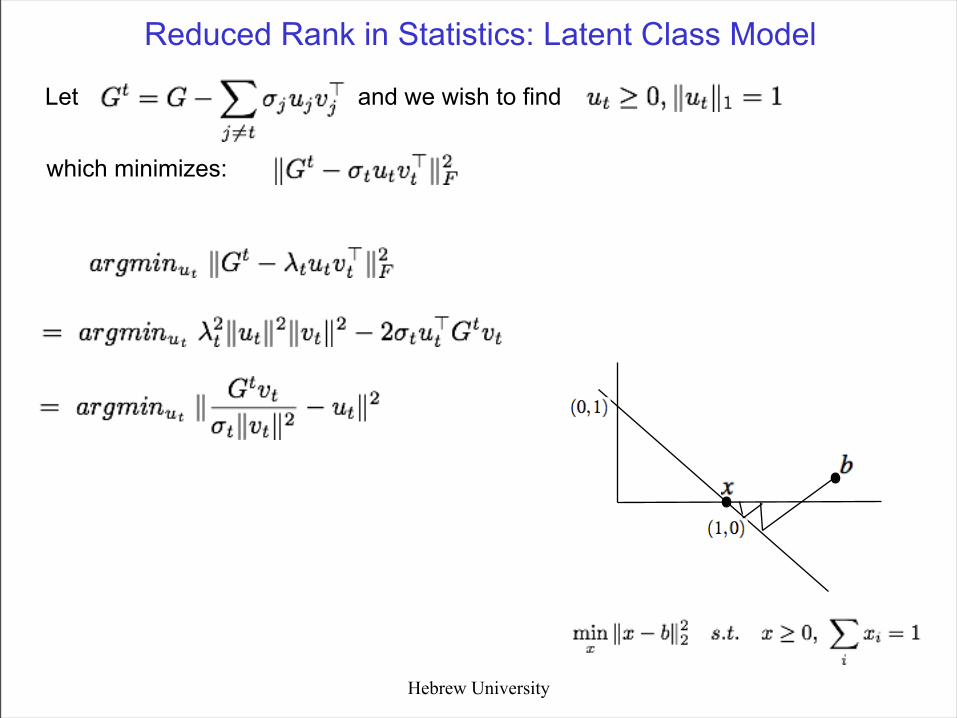
Reduced Rank in Statistics: Latent Class Model
Let and we wish to find
which minimizes:
Hebrew University
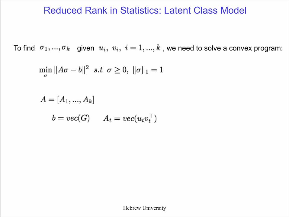
Reduced Rank in Statistics: Latent Class Model
To find given , we need to solve a convex program:
Hebrew University
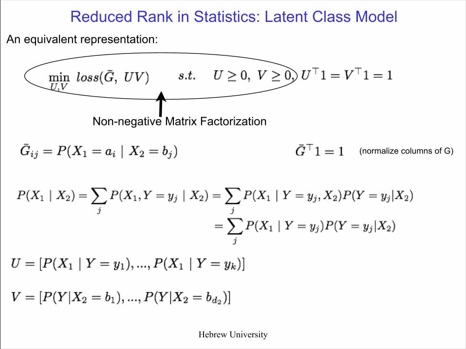
Reduced Rank in Statistics: Latent Class Model
(normalize columns of G)
An equivalent representation:
Non-negative Matrix Factorization
ICML07 Tutorial
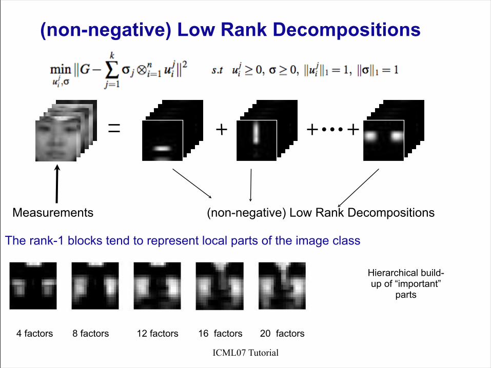
4 factors
Hierarchical build-up of “important”
parts
(non-negative) Low Rank Decompositions
Measurements (non-negative) Low Rank Decompositions
The rank-1 blocks tend to represent local parts of the image class
8 factors 12 factors 16 factors 20 factors
ICML07 Tutorial
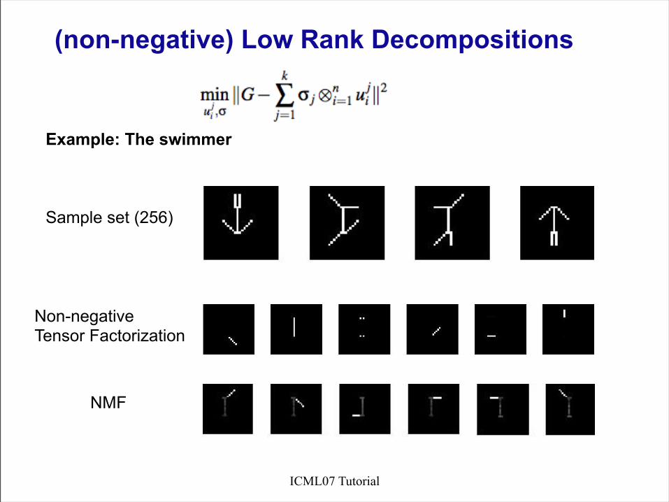
Sample set (256)
Non-negativeTensor Factorization
Example: The swimmer
(non-negative) Low Rank Decompositions
NMF
ICML07 Tutorial 22
Super-symmetric DecompositionsClustering over Hypergraphs
Matrices
ICML07 Tutorial 23
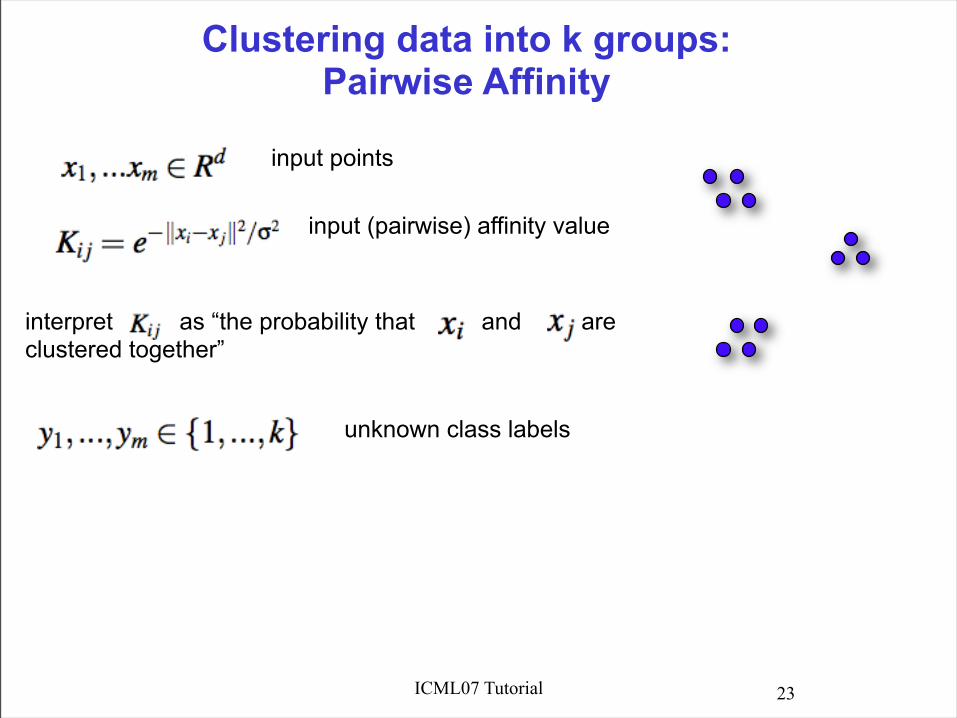
Clustering data into k groups:Pairwise Affinity
input points
input (pairwise) affinity value
interpret as “the probability that and are clustered together”
unknown class labels

ICML07 Tutorial 24
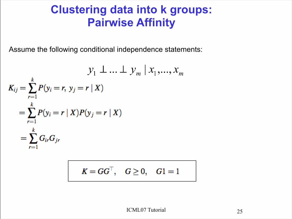
Clustering data into k groups:Pairwise Affinity
input points
input (pairwise) affinity value
interpret as “the probability that and are clustered together”
unknown class labels
A probabilistic view:
probability that belongs to the j’th cluster
What is the (algebraic) relationship between the input matrix K and the desired G?
k=3 clusters, this point does not belong to any cluster in a “hard” sense.
note:
ICML07 Tutorial 25
Clustering data into k groups:Pairwise Affinity
Assume the following conditional independence statements:
ICML07 Tutorial 26
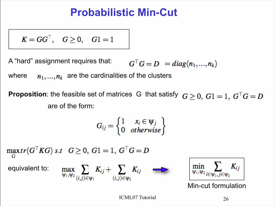
Probabilistic Min-Cut
A “hard” assignment requires that:
where are the cardinalities of the clusters
Proposition: the feasible set of matrices G that satisfy
are of the form:
equivalent to:
Min-cut formulation
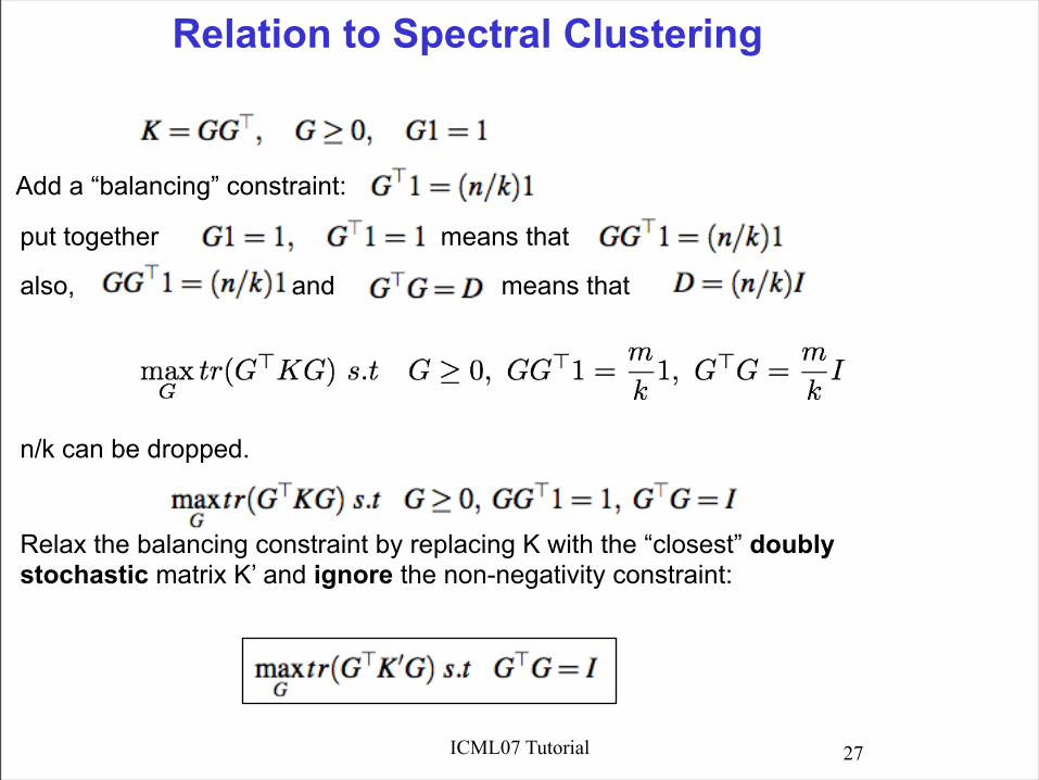
ICML07 Tutorial 27
also, and means that
put together means that
Relation to Spectral Clustering
Add a “balancing” constraint:
n/k can be dropped.
Relax the balancing constraint by replacing K with the “closest” doubly stochastic matrix K’ and ignore the non-negativity constraint:
ICML07 Tutorial 28
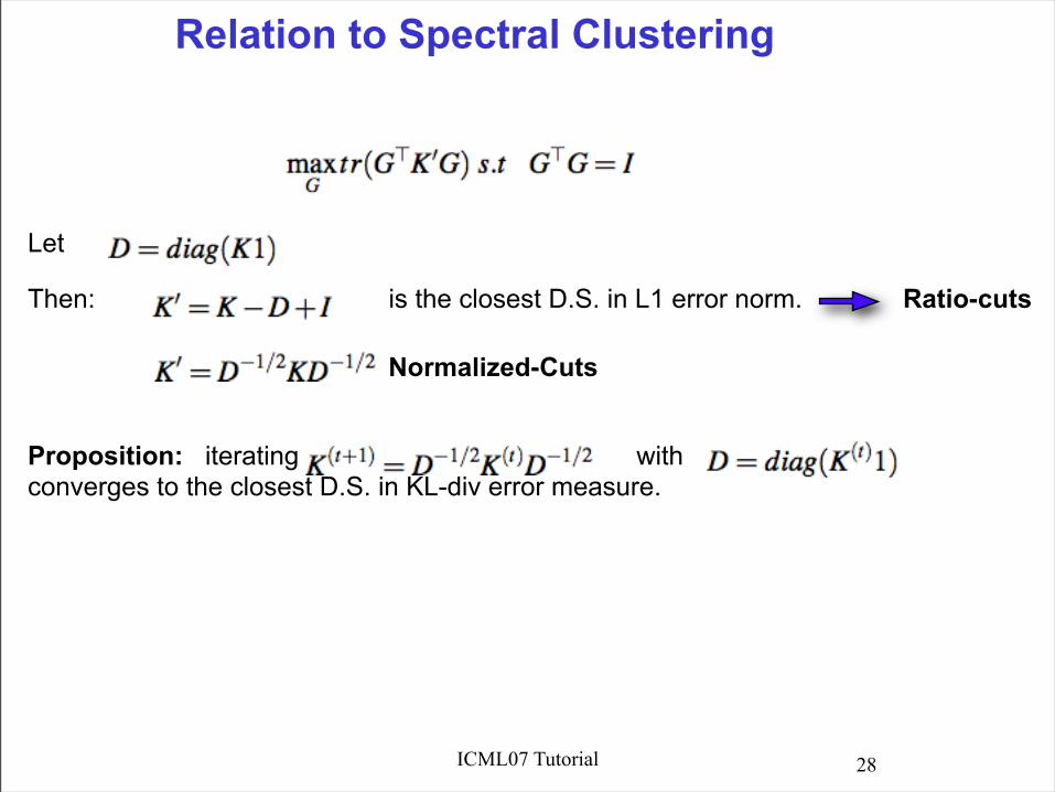
Relation to Spectral Clustering
Let
Then: is the closest D.S. in L1 error norm.
Normalized-Cuts
Ratio-cuts
Proposition: iterating with is converges to the closest D.S. in KL-div error measure.
ICML07 Tutorial 29
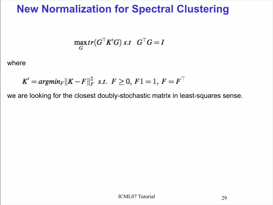
New Normalization for Spectral Clustering
where
we are looking for the closest doubly-stochastic matrix in least-squares sense.

ICML07 Tutorial 30
New Normalization for Spectral Clustering
to find K’ as above, we break this into two subproblems:
use the Von-Neumann successive projection lemma:
ICML07 Tutorial 31
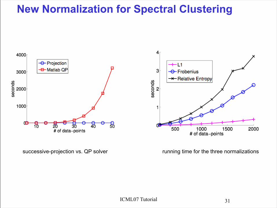
New Normalization for Spectral Clustering
successive-projection vs. QP solver running time for the three normalizations

ICML07 Tutorial 32
New Normalization for Spectral Clustering
UCI Data-sets
Cancer Data-sets
ICML07 Tutorial 33
Super-symmetric DecompositionsClustering over Hypergraphs
Tensors
ICML07 Tutorial
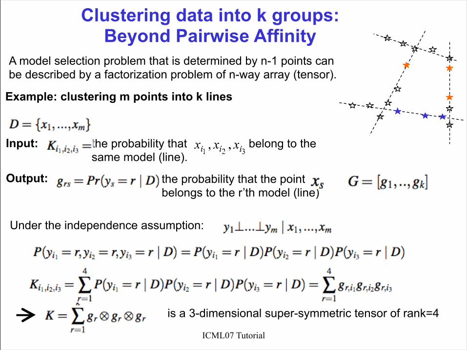
the probability that the point belongs to the r’th model (line)
the probability that belong to the same model (line).
is a 3-dimensional super-symmetric tensor of rank=4
A model selection problem that is determined by n-1 points can be described by a factorization problem of n-way array (tensor).
Under the independence assumption:
Example: clustering m points into k lines
Input:
Output:
Clustering data into k groups:Beyond Pairwise Affinity
ICML07 Tutorial
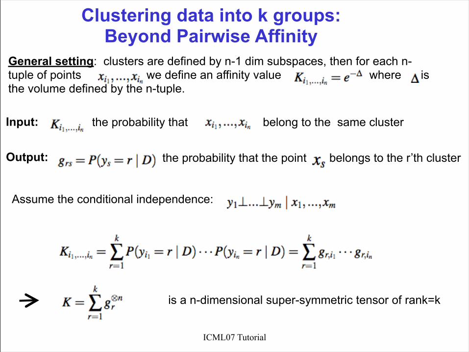
the probability that the point belongs to the r’th cluster
the probability that belong to the same cluster
is a n-dimensional super-symmetric tensor of rank=k
General setting: clusters are defined by n-1 dim subspaces, then for each n-tuple of points we define an affinity value where is the volume defined by the n-tuple.
Assume the conditional independence:
Input:
Output:
Clustering data into k groups:Beyond Pairwise Affinity
ICML07 Tutorial
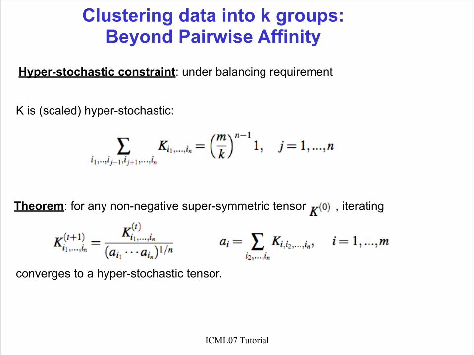
Hyper-stochastic constraint: under balancing requirement
Clustering data into k groups:Beyond Pairwise Affinity
K is (scaled) hyper-stochastic:
Theorem: for any non-negative super-symmetric tensor , iterating
converges to a hyper-stochastic tensor.

ICML07 Tutorial
Example: multi-body segmentation
9-way array, each entry contains The probability that a choice of 9-tupleof points arise from the same model.
Probability:
Model Selection
ICML07 Tutorial
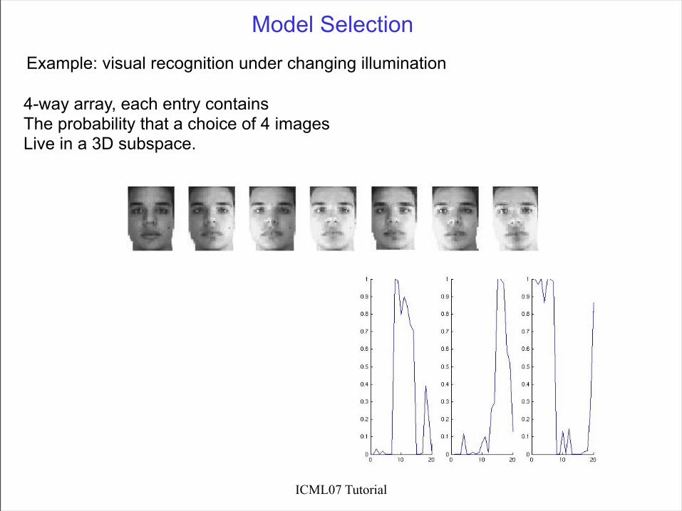
Example: visual recognition under changing illumination
4-way array, each entry contains The probability that a choice of 4 imagesLive in a 3D subspace.
Model Selection

ICML07 Tutorial 39
Partially-symmetric DecompositionsLatent Clustering
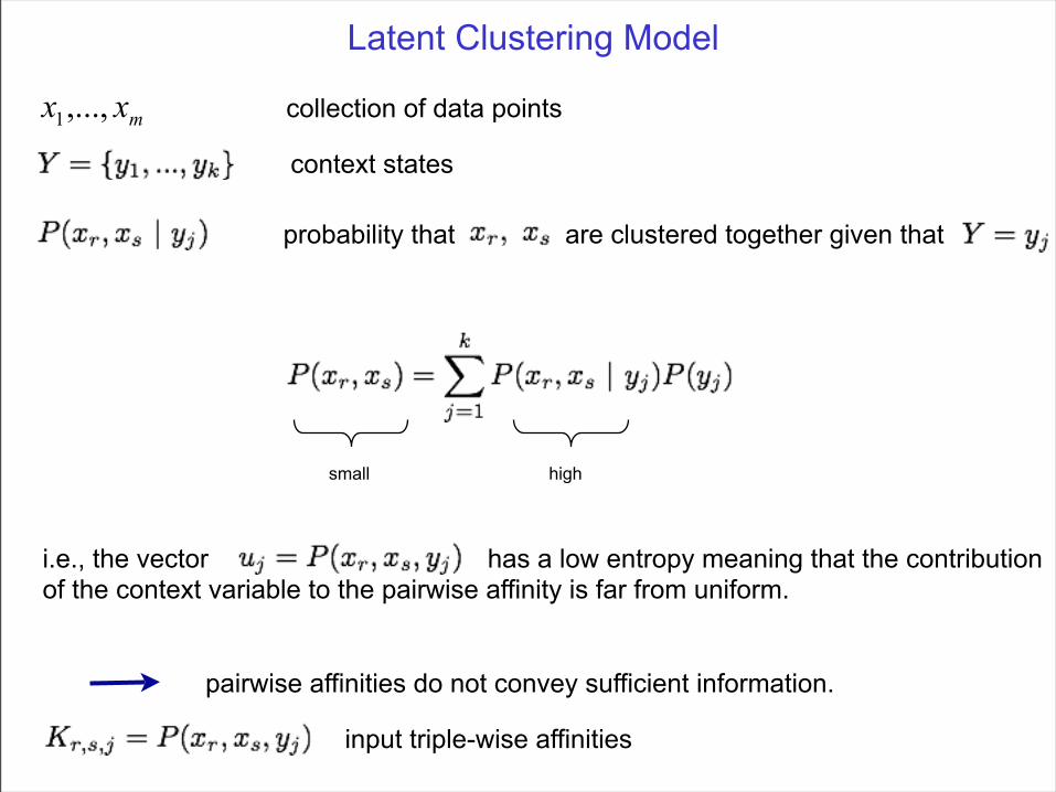
probability that are clustered together given that
Latent Clustering Model
collection of data points
context states
small high
i.e., the vector has a low entropy meaning that the contributionof the context variable to the pairwise affinity is far from uniform.
pairwise affinities do not convey sufficient information.
input triple-wise affinities
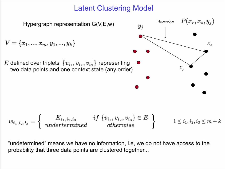
Latent Clustering ModelHyper-edgeHypergraph representation G(V,E,w)
defined over triplets representingtwo data points and one context state (any order)
“undetermined” means we have no information, i.e, we do not have access to the probability that three data points are clustered together...
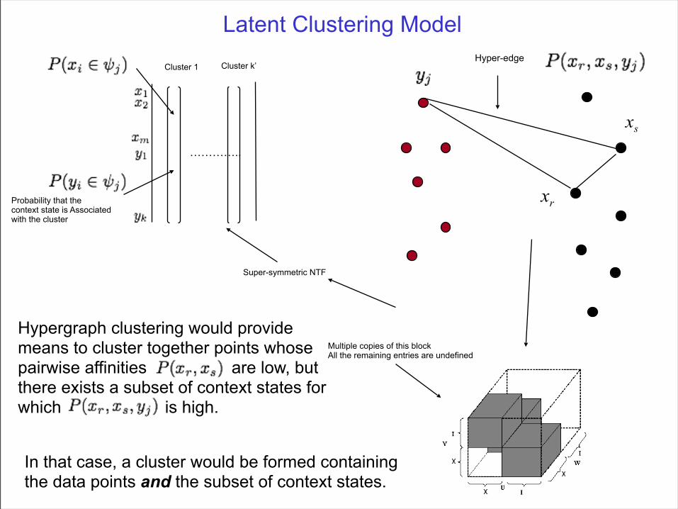
Cluster 1 Cluster k’
…………..
Probability that the context state is Associated with the cluster
Hyper-edge
Multiple copies of this blockAll the remaining entries are undefined
Super-symmetric NTF
Hypergraph clustering would providemeans to cluster together points whosepairwise affinities are low, butthere exists a subset of context states forwhich is high.
In that case, a cluster would be formed containingthe data points and the subset of context states.
Latent Clustering Model

Multiple copies of this blockAll the remaining entries are undefined
Latent Clustering Model

Multiple copies of this blockAll the remaining entries are undefined
Latent Clustering Model
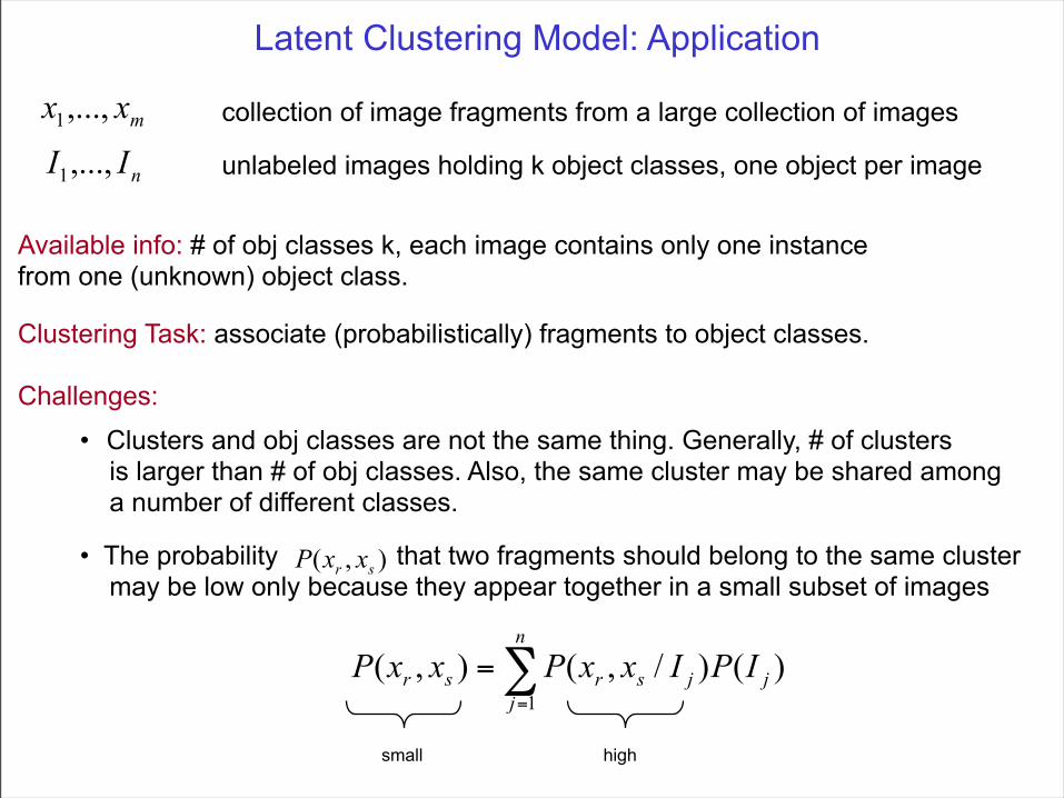
Available info: # of obj classes k, each image contains only one instance from one (unknown) object class.
Latent Clustering Model: Application
collection of image fragments from a large collection of images
Clustering Task: associate (probabilistically) fragments to object classes.
unlabeled images holding k object classes, one object per image
Challenges:
• Clusters and obj classes are not the same thing. Generally, # of clusters is larger than # of obj classes. Also, the same cluster may be shared among a number of different classes.
• The probability that two fragments should belong to the same cluster may be low only because they appear together in a small subset of images
small high
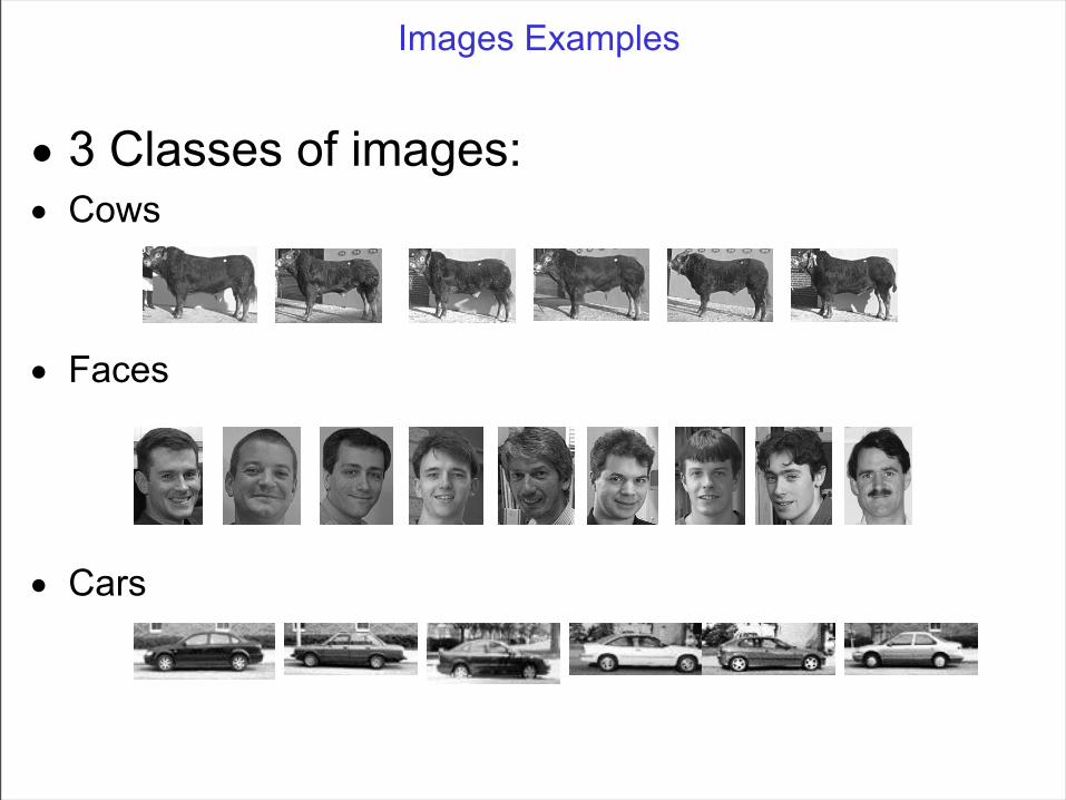
• 3 Classes of images:• Cows
• Faces
• Cars
Images Examples
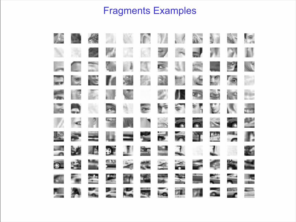
Fragments Examples

Examples of Representative Fragments

Leading Fragments Of Clusters
Cluster 1
Cluster 2
Cluster 3
Cluster 4
Cluster 5
Cluster 6
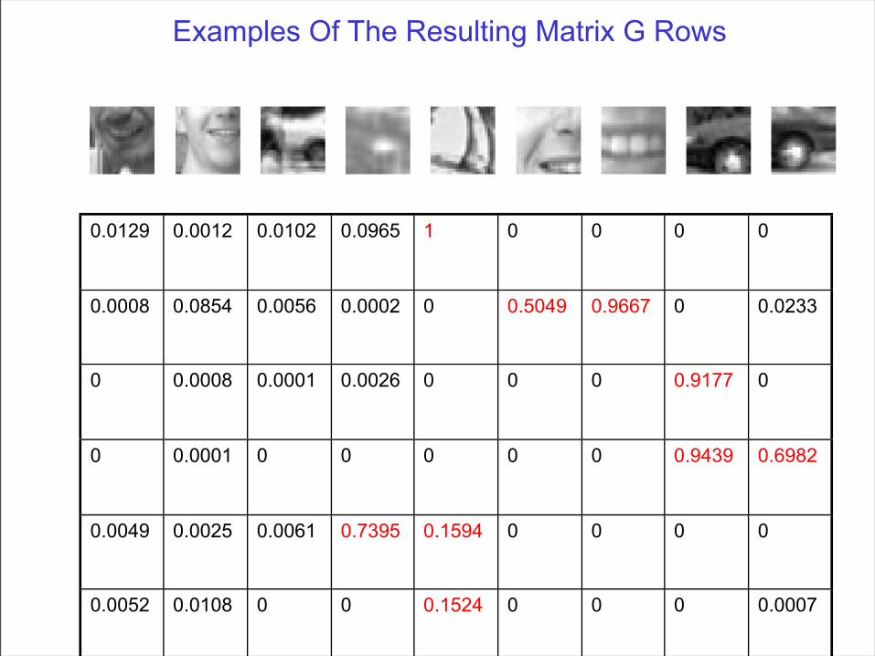
Examples Of The Resulting Matrix G Rows
0.0129 0.0012 0.0102 0.0965 1 0 0 0 0
0.0008 0.0854 0.0056 0.0002 0 0.5049 0.9667 0 0.0233
0 0.0008 0.0001 0.0026 0 0 0 0.9177 0
0 0.0001 0 0 0 0 0 0.9439 0.6982
0.0049 0.0025 0.0061 0.7395 0.1594 0 0 0 0
0.0052 0.0108 0 0 0.1524 0 0 0 0.0007
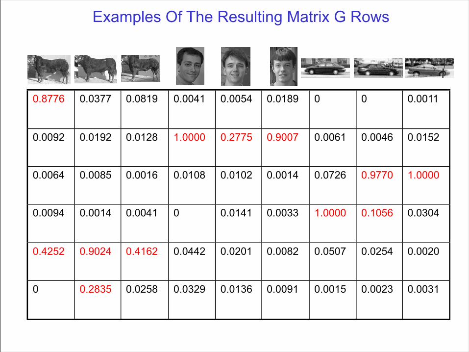
Examples Of The Resulting Matrix G Rows
0.8776 0.0377 0.0819 0.0041 0.0054 0.0189 0 0 0.0011
0.0092 0.0192 0.0128 1.0000 0.2775 0.9007 0.0061 0.0046 0.0152
0.0064 0.0085 0.0016 0.0108 0.0102 0.0014 0.0726 0.9770 1.0000
0.0094 0.0014 0.0041 0 0.0141 0.0033 1.0000 0.1056 0.0304
0.4252 0.9024 0.4162 0.0442 0.0201 0.0082 0.0507 0.0254 0.0020
0 0.2835 0.0258 0.0329 0.0136 0.0091 0.0015 0.0023 0.0031
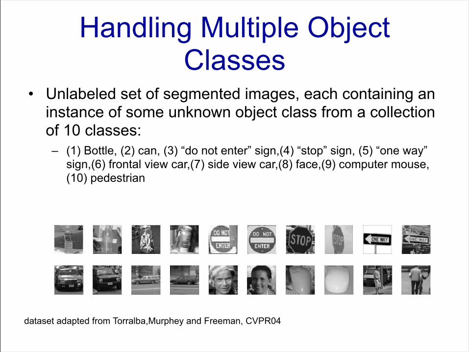
Handling Multiple Object Classes
• Unlabeled set of segmented images, each containing an instance of some unknown object class from a collection of 10 classes:– (1) Bottle, (2) can, (3) “do not enter” sign,(4) “stop” sign, (5) “one way”
sign,(6) frontal view car,(7) side view car,(8) face,(9) computer mouse,(10) pedestrian
dataset adapted from Torralba,Murphey and Freeman, CVPR04

Clustering Fragments
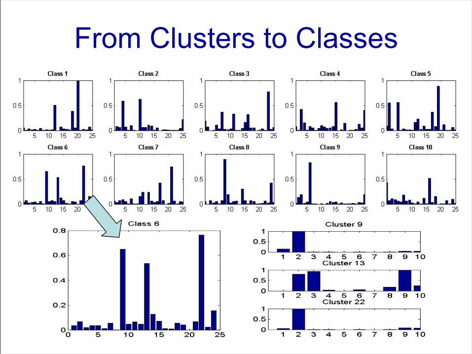
From Clusters to Classes
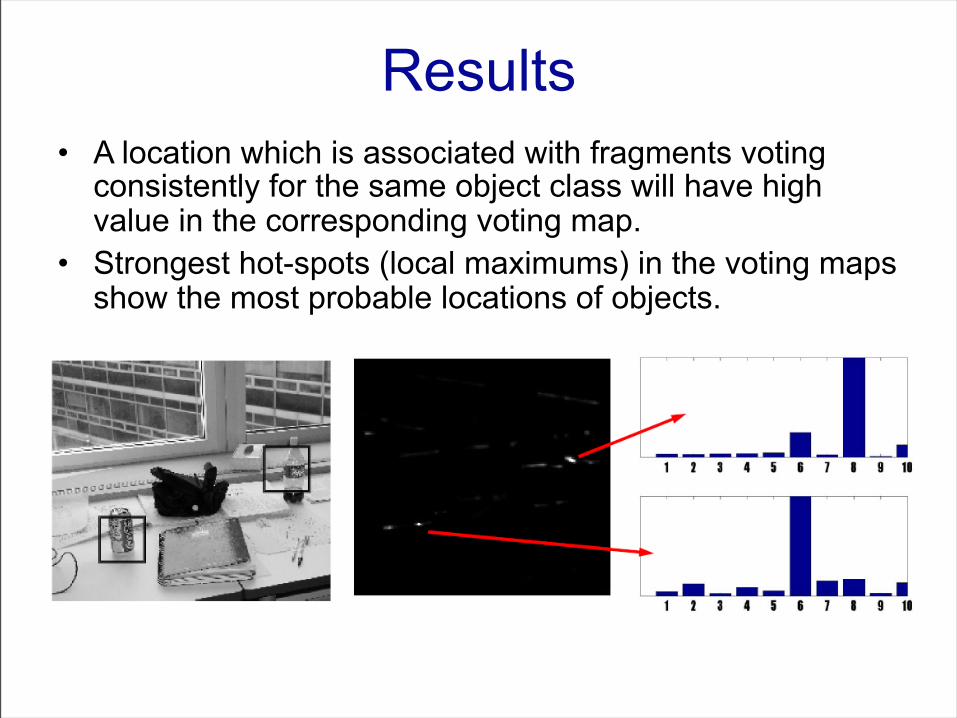
Results• A location which is associated with fragments voting
consistently for the same object class will have high value in the corresponding voting map.
• Strongest hot-spots (local maximums) in the voting maps show the most probable locations of objects.
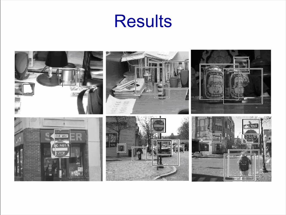
Results

ICML07 Tutorial 57
Applications of NTFlocal features for object class recognition

Hebrew University 58
Find a good and efficient collection of filters that captures the essence of an object class of images.
1) Use a large pre-defined bank of filters which:
Object Class Recognition using FiltersGoal:Two main approaches:
Rich in variability.
Efficiently convolved with an image.
Viola-Jones Hel-Or
2) Use filters as basis vectors spanning a low-dimensional vector space which best fits the training images.
PCA, HOSVD – “holistic”
NMF – “sparse”
The classification algorithm selects a subset of filters which is most discriminatory.

Hebrew University 59
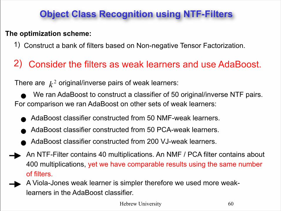
The optimization scheme:
Object Class Recognition using NTF-Filters
Construct a bank of filters based on Non-negative Tensor Factorization.
1)
Consider the filters as weak learners and use AdaBoost.2)
Bank of Filters:
We take the difference between the two convolutions (original - inverse).
We perform an NTF of k factors to approximate the set of original images.
We perform an NTF of k factors to approximate the set of inverse images.
There are filters Every filter is a pair of original/inverse factor.
Original/Inverse pair for face recognition
Hebrew University 60
There are original/inverse pairs of weak learners:
The optimization scheme:Construct a bank of filters based on Non-negative Tensor Factorization.1)
Consider the filters as weak learners and use AdaBoost.2)
We ran AdaBoost to construct a classifier of 50 original/inverse NTF pairs.For comparison we ran AdaBoost on other sets of weak learners:
AdaBoost classifier constructed from 50 NMF-weak learners.
AdaBoost classifier constructed from 50 PCA-weak learners.
AdaBoost classifier constructed from 200 VJ-weak learners.
An NTF-Filter contains 40 multiplications. An NMF / PCA filter contains about 400 multiplications, yet we have comparable results using the same number of filters.A Viola-Jones weak learner is simpler therefore we used more weak-learners in the AdaBoost classifier.
Object Class Recognition using NTF-Filters
Hebrew University 61
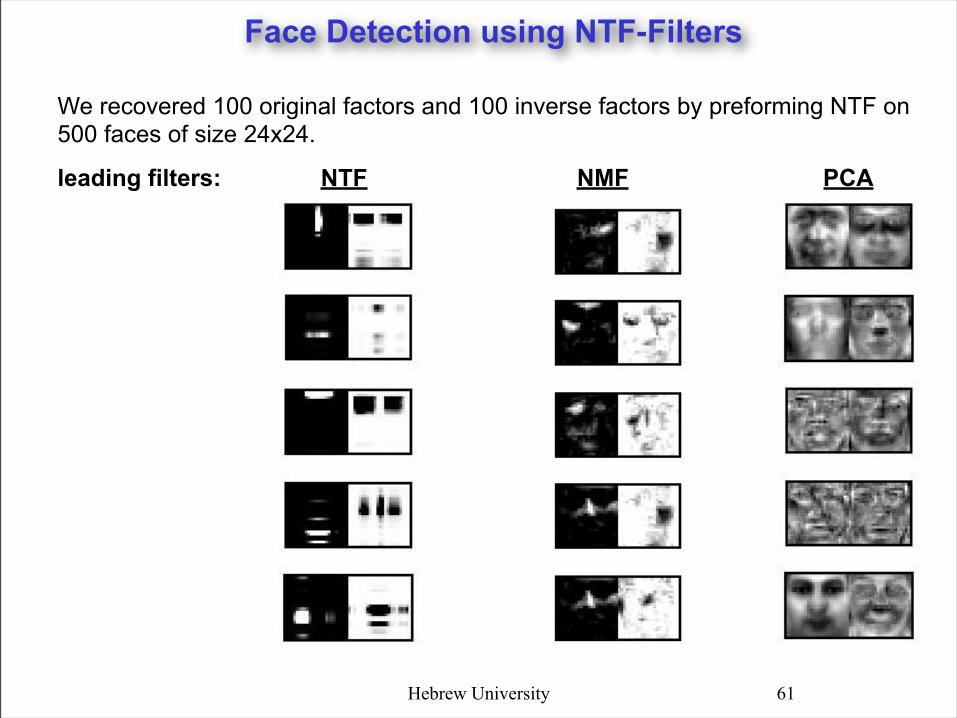
Face Detection using NTF-Filters
leading filters: NTF NMF PCA
We recovered 100 original factors and 100 inverse factors by preforming NTF on 500 faces of size 24x24.
Hebrew University 62
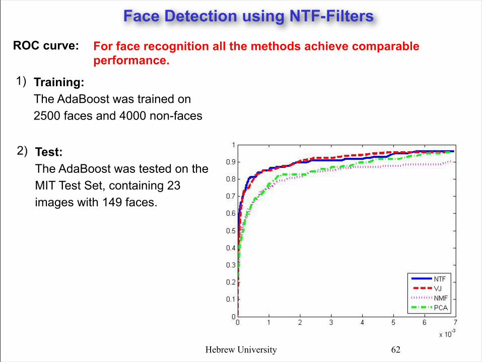
ROC curve:
Training: The AdaBoost was trained on 2500 faces and 4000 non-faces
1)
For face recognition all the methods achieve comparable performance.
Face Detection using NTF-Filters
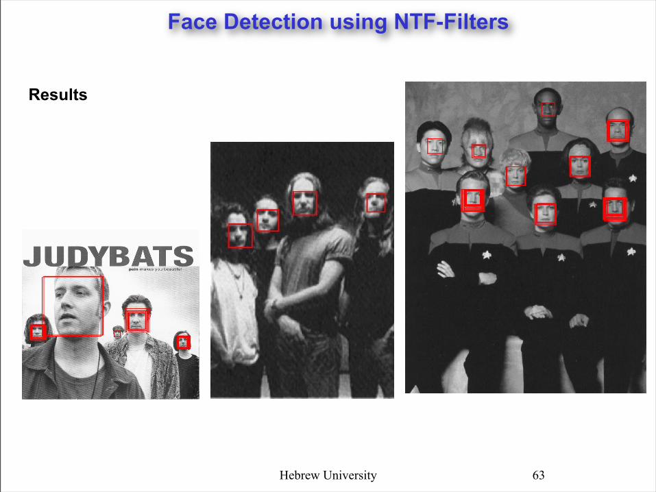
Test: The AdaBoost was tested on the MIT Test Set, containing 23 images with 149 faces.
2)
Hebrew University 63
Results
Face Detection using NTF-Filters
Hebrew University 64
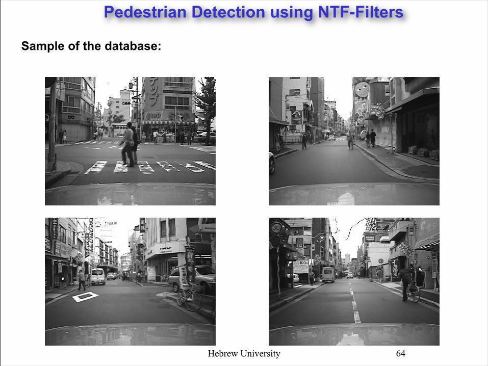
Sample of the database:
Pedestrian Detection using NTF-Filters
Hebrew University 65
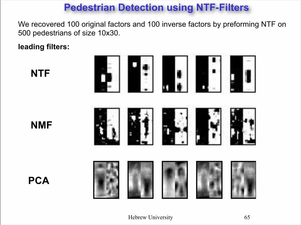
PCA
NMF
NTF
Pedestrian Detection using NTF-Filters
leading filters:
We recovered 100 original factors and 100 inverse factors by preforming NTF on 500 pedestrians of size 10x30.

Hebrew University 66
ROC curve:
Training: The AdaBoost was trained on 4000 pedestrians and 4000 non-pedestrains.
1)
For pedestrian detection NTF achieves far better performance than the rest.
Test: The AdaBoost was tested on 20 images with 103 pedestrians.
2)
Pedestrian Detection using NTF-Filters
Hebrew University 67
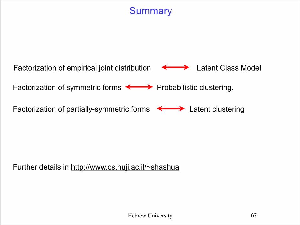
Summary
Factorization of symmetric forms Probabilistic clustering.
Factorization of empirical joint distribution Latent Class Model
Factorization of partially-symmetric forms Latent clustering
Further details in http://www.cs.huji.ac.il/~shashua
ICML07 Tutorial
END
Recommended