1
The Thomson Effect and the Ideal Equation on Thermoelectric Coolers
HoSung Lee
Mechanical and Aeronautical Engineering, Western Michigan University,
1903 W. Michigan Ave, Kalamazoo, Michigan 49008, USA
Office (269) 276-3429
Fax (269) 276-3421
Abstract
The formulation of the classical basic equations for a thermoelectric cooler from the
Thomson relations to the non-linear differential equation with Onsager’s reciprocal relations was
performed to basically study the Thomson effect in conjunction with the ideal equation. The
ideal equation is obtained when the Thomson coefficient is assumed to be zero. The exact
solutions derived for a commercial thermoelectric cooler module provided the temperature
distributions including the Thomson effect. The positive Thomson coefficient led to a slight
improvement on the performance of the thermoelectric device while the negative Thomson
coefficient led to a slight declination of the performance. The comparison between the exact
solutions and the ideal equation on the cooling power and the coefficient of performance over a
wide range of temperature differences showed close agreement. In conclusion, the Thomson
effect is small for typical commercial thermoelectric coolers and the ideal equation effectively
predicts the performance.
Keywords: thermoelectrics, thermoelectricity, thermoelectric coolers, thermoelectric
refrigerators, thermoelectric devices, Thomson relations, Thomson effect
Nomenclature A cross-sectional area of thermoelement (m2)
COP the coefficient of performance, dimensionless
pc specific heat capacity (J/kgK)
E
electric field vector (V/m) I electric current (A)
j
electric current density vector (A/m2)
j electric current density (A/m2)
iJ arbitrary quantities
K thermal conductance (W/K)
L length of thermoelement (m)
k thermal conductivity (W/mK)
q
heat flux vector (W/m2)
q heat generation (W/m3)
cQ cooling power (W)
2
1Q cooling power (W)
R electrical resistivity ()
ijR kinetic coefficients
gens entropy generation per unit volume (J/m3K)
gens entropy generation per unit time and unit volume (J/m3K)
genS entropy generation (J/K)
genS entropy generation per unit time (W/K)
T absolute temperature (K)
cT low junction temperature (K)
hT high junction temperature (K)
1T low junction temperature (K)
2T high junction temperature (K)
T temperature difference (K), 12 TT
V volume (m3)
W work per unit time RITIW 2
x distance of thermoelement leg (m)
ix arbitrary quantities
iX arbitrary quantities: txi
Greek symbols
Seebeck coefficient (V/K)
dimensionless number LAkdTdIT 2
dimensionless number LTAkRI 2
the ratio of T to T2
density (kg/m3)
electric resistivity (m)
Thomson coefficient (V/K)
dimensionless temperature 121 TTTT
dimensionless distance Lx
1 dimensionless cooling power LTAkQ 11
dimensionless Peltier cooling LAkIT1
dimensionless work LTAkW
3
1. Introduction
Thermoelectric phenomena are useful and have drawn much attention since the discovery of
the phenomena in the early nineteenth century. The barriers to applications were low efficiencies
and the availability of materials. In 1821, Thomas J. Seebeck discovered that an electromotive
force or potential difference could be produced by a circuit made from two dissimilar wires when
one junction was heated . This is called the Seebeck effect. In 1834, Jean Peltier discovered the
reverse process that the passage of an electric current through a thermocouple produces heating
or cooling depended on its direction [1]. This is called the Peltier effect (or Peltier cooling). In
1854, William Thomson discovered that if a temperature difference exists between any two
points of a current-carrying conductor, heat is either absorbed or liberated depending on the
direction of current and material [2]. This is called the Thomson effect (or Thomson heat). These
three effects are called the thermoelectric effects. Thomson also developed important
relationships between the above three effects with the reciprocal relations of the kinetic
coefficients (or sometimes the so-called symmetry of the kinetic coefficients) under a peculiar
assumption that the thermodynamically reversible and irreversible processes in thermoelectricity
are separable [2]. The relationship developed is called the Thomson (or Kelvin) relations. The
necessity for the assumption remained an objection to the theory until the advent of the new
thermodynamics [3-6]. The relationship was later completely confirmed by experiments to be
essentially a consequence of the Onsager’s Reciprocal Principle in 1931 [3].
As supported by Onsager’s Principle, the Thomson relations provide a simple expression for
Peltier cooling, which is the product of the Seebeck coefficient, the temperature at the junction,
and the current. This Peltier cooling is the principal thermoelectric cooling mechanism. There are
two counteracting phenomena, which are the Joule heating and the thermal conduction. The net
cooling power is the Peltier cooling minus these two effects. Actually the Joule heating affects
the thermal conduction and consequently the Peltier cooling is subtracted only by the thermal
conduction. Expressing the net cooling power in terms of the heat flux vector q
gives [7]
TkjTq
(1)
This is the most important formula, where is the Seebeck coefficient, T the absolute
temperature, j
the current density and k the thermal conductivity. Equation (1) appears simple,
but the interpretation was somewhat formidable because the T in the equation was obtained by
conjecture and the reciprocal relations. In fact, the three thermoelectric effects that are known to
be reversible are effectively combined into the T [8-10]. The second term gives the thermal
conduction that is obviously irreversible. A steady-state heat diffusion equation is given by [7]
02 TjdT
dTjTk
(2)
where is the electrical resistivity. Equation (2) is a non-linear differential equation. The
Thomson coefficient is given by
4
dT
dT
(3)
In order to obtain the net cooling power, Equation (2) is first solved for the thermal
conduction including the Joule heating and then Equation (1) can give the cooling power at the
junction. It is often assumed [8,9,10,16,17] that the Thomson effect was absent or negligible or,
in other words, was independent of temperature. In such a case, Equation (2) becomes an
ordinary differential equation and can be easily solved for the thermal conduction and then
Equation (1) yields a well-known equation as
chcc TTKRIITQ 2
2
1 (4)
where cQ is the cooling power, I the current, cT the low junction temperature, hT the high
junction temperature, R the electrical resistance, and K the thermal conductance. Equation (4) is
called the ideal equation and has been widely used in science and industry [8, 10, 15, 16] often
with a fair agreement with the experiments [9, 13].
The third term in Equation (2) was regarded as the Thomson effect. The influence of the
Thomson effect was discussed in the literature [11-14] by numerically solving Equation (2), in
which the Seebeck coefficient was dependent of temperature. The exact solutions of Equation
(2) assuming that the Thomson coefficient is constant indicated that the Thomson effect would
improve the performance significantly [12, 13]. More realistic work on the Thomson coefficient
assuming that dTd is a linear function of temperature was numerically conducted using a
finite difference method and also experimentally compared with a commercial module showing
slight improvement on the performance [13]. Numerical simulations on the Thomson effect
using CFD software ANSYS for miniature thermoelectric coolers revealed that the cooling
power can be improved by a factor of 5 - 7% [14] by including the Thomson effect. There is an
experimental work [18] showing that the Thomson effect is responsible for reduction of the
figure of merit on a thermoelectric generator with an increase of temperature difference, whereas
the researchers anticipated enhancement of the figure of merit on a thermoelectric cooler. There
were attempts [19, 20] to improve the performance of thermoelectric devices by optimizing the
temperature dependence of the material properties wherein the Thomson effect was taken into
account although the improvement could not be demonstrated by the measurements. There is a
rigorous numerical analysis [21] for emerging materials and large temperature gradients in
thermoelectric generators how well the ideal equation predicts the exact solutions including the
Thomson effect. It is analytically proven [21] that the ideal equation produces the exact solution
output power and efficiency despite its limiting assumptions if an integral-averaged Seebeck
coefficient is used.
From the review of the above experimental and theoretical work, the present author feels
that further realistic studies are required to clarify the Thomson effect related to the ideal
equation in temperature distributions, particularly in the positive and negative Thomson
coefficients. The present work studies the Thomson effect in conjunction with the ideal equation
from the formulation of the basic equations to the numerical simulations in light of a real
commercial thermoelectric module.
5
2. Formulation of Basic Equations
2.1 Onsager’s Reciprocal Relations
The second law of thermodynamics with no mass transfer (S = 0) in an isotropic substance
provides an expression for the entropy generation.
2
1T
QSgen
> 0 (5)
Suppose that the derivatives of the entropy generation sgen per unit volume with respect to
arbitrary quantities xi are quantities Ji [5, 8] as
i
i
genJ
x
s
(6)
At maximum sgen, Ji is zero. Accordingly, at the state close to equilibrium (or maximum), Ji
is small [4]. The entropy generation per unit time and unit volume is
iigen
gen Jt
x
t
ss
(7)
We want to express txi as iX . Then, we have
iigen JXs (8)
The iX are usually a function of iJ . Onsager [3] stated that if iJ were completely
independent, we should have the relation, expanding iX in the powers of Ji and taking only linear
terms [7]. The smallness of iJ in practice allows the linear relations being sufficient.
j
jiji JRX (9)
where Rij are called the kinetic coefficients. Hence, we have
i
iigen JXs (10)
It is necessary to choose the quantities iX in some manner, and then to determine the Ji.
The iX and Ji are conveniently determined simply by means of the formula for the rate of change
of the total entropy generation.
6
dVJXSi
iigen > 0 (11)
For two terms, we have
dVJXJXSgen 2211 > 0 (12)
And
2121111 JRJRX (13)
2221212 JRJRX (14)
From these equations, one can assert that the kinetic coefficients are symmetrical with
respect to the suffixes 1 and 2.
2112 RR (15)
which is called the reciprocal relations.
2.2 Basic Equations
Let us consider a non-uniformly heated thermoelectric material. For an isotropic substance,
the continuity equation for a constant current gives
0 j
(16)
The electric field E
is affected by the current density j
and the temperature gradient T
.
The coefficients are known according to the Ohm’s law and the Seebeck effect [7]. The field is
then expressed as
TjE
(17)
where is the electrical resistivity and is the Seebeck coefficient. Solving for the current
density gives
TEj
1 (18)
The heat flux q
is also affected by the both field E
and temperature gradient T
. However,
the coefficients were not readily attainable at that time. Thomson in 1854 arrived at the
relationship assuming that thermoelectric phenomena and thermal conduction are independent.
Later, Onsager [3] supported that relationship by presenting the reciprocal principle which was
7
experimentally proved but failed the phenomenological proof [6]. Here we derive the Thomson
relationship using Onsager’s principle. The heat flux with arbitrary coefficients is
TCECq
21 (19)
The general heat diffusion equation is
t
Tcqq p
(20)
For steady state, we have
0 qq
(21)
where q is expressed by [7]
TjjjEq
2 (22)
Expressing Equation (5) with Equation (21) in a manner that the heat flux gradient q has a
minus sign, the entropy generation per unit time will be
dVqqTT
QSgen
12
1
(23)
Using Equation (22), we have
dVT
q
T
jESgen
(24)
The second term is integrated by parts, using the divergence theorem and noting that the
fully transported heat does not produce entropy since the volume term cancels out the surface
contribution [7]. Then, we have
dVT
Tq
T
jESgen
2
(25)
If we take j
and q
as 1X and 2X , then the corresponding quantities 1J and 2J are the
components of the vectors TE and 2TT
[7]. Accordingly, as shown in Equations (13) and
(14) with Equation (19), we have

8
2
211
T
TT
T
ETj
(26)
2
2
21T
TTC
T
ETCq
(27)
where the reciprocal relations in Equation (15) gives
2
1
1TTC
(28)
Thus, we have TC 1 . Inserting this and Equation (17) into (27) gives
TT
CjTq
2
2 (29)
We introduce the Wiedemann-Franz law that is TkLo , where Lo is the Lorentz number
(constant). Expressing k as LoT/, we find that the coefficient TC 2
2 is nothing more than
the thermal conductivity k. Finally, the heat flow density vector (heat flux) is expressed as
TkjTq
(30)
This is the most essential equation for thermoelectric phenomena. The second term pertains
to the thermal conduction and the term of interest is the first term, which gives the thermoelectric
effects: directly the Peltier cooling but indirectly the Seebeck effect and the Thomson heat [8, 9,
10]. Inserting Equations (17) and (30) into Equation (25) gives
dV
T
Tk
T
jS gen
2
22
> 0 (31)
The entropy generation per unit time for the irreversible processes is indeed greater than
zero since and k are positive. Note that the Joule heating and the thermal conduction in the
equation are indeed irreversible. This equation satisfies the requirement for Onsager’s reciprocal
relations as shown in Equation (12). Substituting Equations (22) and (30) in Equation (21) yields
02 TjdT
dTjTk
(32)
The Thomson coefficient , originally obtained from the Thomson relations, is written
9
dT
dT
(33)
In Equation (32), the first term is the thermal conduction, the second term is the Joule
heating, and the third term is the Thomson heat. Note that if the Seebeck coefficient is
independent of temperature, the Thomson coefficient is zero and then the Thomson heat is
absent.
2.3 Exact Solutions
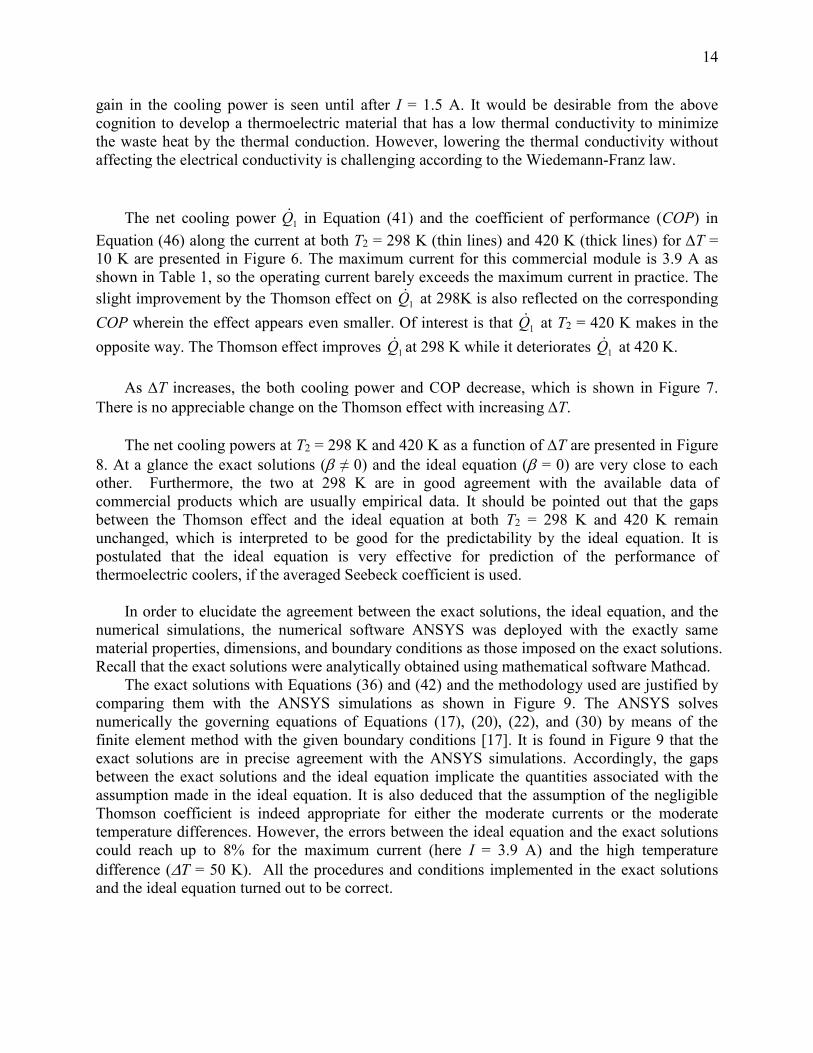
Let us consider one of p- and n-type thermoelements as shown in Figure 1, knowing that p-
and n-type thermoelements produce the same results if the materials and dimensions are assumed
to be similar. Equation (32) for one dimensional analysis at steady state gives the non-linear
differential governing equation as
02
2
2
2
kA
I
dx
dTT
Ak
dT
dI
dx
Td
(34)
where A is the cross-sectional area of the thermoelement. We want to make it dimensionless. The
boundary conditions will be T(0) = T1 and T(L) = T2. Then, Let
12
1
TT
TT
and
L
x (35)
where L is the element length. Then, the dimensionless differential equation is
0112
2
d
d
d
d (36)
where the dimensionless numbers are defined as follows. The boundary condition will be that
00 and 11 . Equation (36) was formulated on the basis of the high junction
temperature T2 to meet the commercial products.
L
TAk
TdT
dIT
2
(37)
where is the ratio of the Thomson heat to the thermal conduction. Note that is not a function
of T.
10
L
TAk
RI
2
(38)
where is the ratio of the Joule heating to the thermal conduction.
2T
T (39)
where is the ratio of temperature difference to the high junction temperature. The temperature
difference is
12 TTT (40)
where is the high junction temperature T2 minus the low junction temperature T1. Therefore,
T1 is a function of since T2 is fixed. The cooling power at the cold junction using Equation
(30) is
0
111
xdx
dTkAITTQ (41)
where the first term is the Peltier cooling and the second term is the thermal conduction. It has
been customary in the literature for the exact solution wherein the Seebeck coefficient is
evaluated at the cold junction temperature T1. The dimensionless cooling power is expressed
0
1
1
d
d (42)
where 1 is the dimensionless cooling power, which is
LTAk
Q
1
1
(43)
and the dimensionless Peltier cooling is
LAk
IT1 (44)
The work per unit time gives RITIW 2 [10]. Then the dimensionless work per unit
time is expressed by
(45)
11
where LTAk
W
. Then, the coefficient of performance (COP) for the thermoelectric cooler
is determined as the cooling power over the work as
1COP (46)
Equation (36) can be exactly solved for the temperature distributions conveniently with
mathematical software Mathcad and then the cooling power of Equation (41) can be obtained,
which are the exact solutions including the Thomson effect.
2.4 The Ideal Equation
According to the assumption made by the both Thomson relations and Onsager’s reciprocal
relations, the thermoelectric effects and the thermal conduction in Equation (30) are completely
independent, which implies that each term may be separately dealt with. In fact, separately
dealing with the reversible processes of the three thermoelectric effects yielded the Peltier
cooling of the TI in the equation [8-10]. However, under the assumption that the Thomson
coefficient is negligible or the Seebeck coefficient is independent of temperature, Equation (34)
easily provides the exact solution of the temperature distribution. Then, Equation (41) with the
temperature distribution for the cooling power at the cold junction reduces to
12
2
112
1TT
L
AkRIITTQ avg (47)
which appears simple but is a robust equation with a usually good agreement with experiments
and with comprehensive applications in science and industry. This is here called the ideal
equation. The ideal equation assumes that the Seebeck coefficient be evaluated at the average
temperature of T 15, 16] as a result of the internal phenomena being imposed on the surface
phenomena.
3. Results and Discussion
In order to realistically study the Thomson effect on the temperature distributions with the
temperature dependent Seebeck coefficient, a real commercial module of Laird CP10-127-05
was chosen. Both the temperature dependent properties and the dimensions for the module were
provided by the manufacturer, which are shown in Table 1 and the temperature dependent
Seebeck coefficient is graphed in Figure 2.
Table 1 Maximum values, Dimensions, and the Properties for a Commercial Module
TEC Module (Laird CP10-127-05) at 25°C
Tmax (°C) 67
12
Imax (A) 3.9
Qmax (W) 34.3
L (mm), element length 1.253
A (mm2), cross-sectional area 1
# of Thermocouples 127
(T), (V/K) 0.2068T+138.78, 250 K < T< 350 K
(T), (V/K) −0.2144T+281.02, 350 K < T < 450 K
cmat 27 °C 1.01 × 10⁻³
k (W/cmK) at 27 °C 1.51 × 10⁻²
Module size 30 × 30 × 3.2 mm
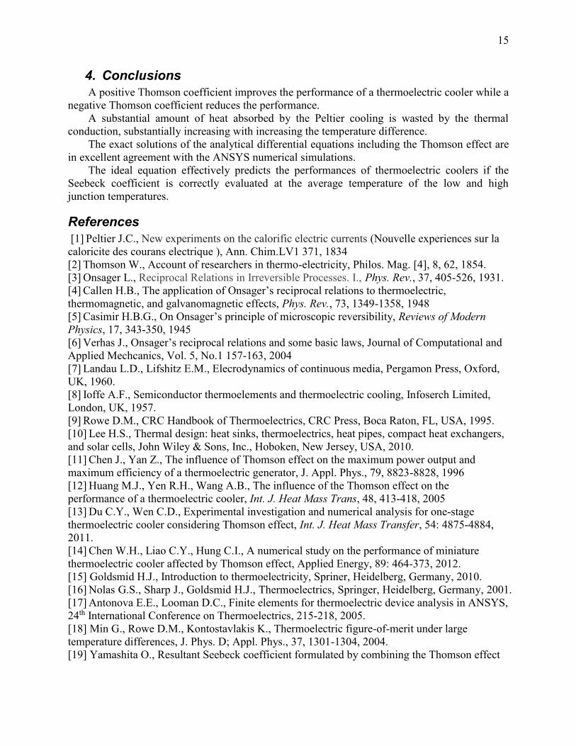
To reveal the Thomson effect, only the Seebeck coefficients are considered to be dependent
of the temperature while the electrical resistivity and the thermal conductivity are constant as
shown in Table 1. In Figure 2, the Seebeck coefficient increases with increasing the temperature
up to about 350 K and then decreases with increasing the temperature, so that there is a peak
value. For the feasible solution with the non-linear differential equation, the linear curve fits for
the Seebeck coefficient were used in the present work. In Figure 2, the linear curve fit of the first
part for a range from 250 K to 350 K was used in the present work, while the other linear curve
fit of the second part for the range from 350 K to 450 K was used separately. The linear curve
fits of the two parts are shown in Table 1. Some reports [11-14] illustrated used only the
monotonically increasing Seebeck coefficients. Therefore, the negative slope of the Seebeck
coefficient was not presented. As mentioned previously, the absolute values of the temperature
dependent Seebeck coefficients for p- and n-type elements are assumed to be the same, but the
sign of n-type element’s coefficient is negative while the sign of p-type element’s coefficient is
positive. In reality, the Seebeck coefficients in the p- and n-type elements are different as the
absolute values vary with temperature. Figure 2 would be the arithmetic average of the two. By
doping technique (intentionally introducing impurities into a pure semiconductor), n-type
semiconductor carries predominantly free electrons moving to the opposite direction of current
applied (which causes the negative sign of the Seebeck coefficient), while p-type semiconductor
carries free holes in the same manner but moving to the same direction of current applied (which
causes the positive sign). Likewise, p- and n-type thermoelements can be arranged electrically in
series and thermally in parallel to form a module. The number of electrons and holes can be
controlled through the introduction of impurities (doping), which are called donors or acceptors.
The dimensionless differential equation, Equation (36), was developed on the basis of a
fixed high junction temperature T2 so that the low junction temperature T1 decreases as T
increases. in Equation (37) is the dimensionless number indicating approximately the ratio of
the Thomson heat to the thermal conduction. is a function only of the slope dTd and the
current I. Equation (36) with the given boundary conditions was solved for the temperature
distributions conveniently using mathematical software Mathcad.
A typical value of = 0.2 was obtained for the commercial product at T2 = 298 K and Imax =
3.9 A. And a hypothetical value of that is fivefold larger than the typical value of 0.2 was
used in order to closely examine the Thomson effect. in Equation (38) is the dimensionless
number indicating approximately the ratio of the Joule heating to the thermal conduction.
13
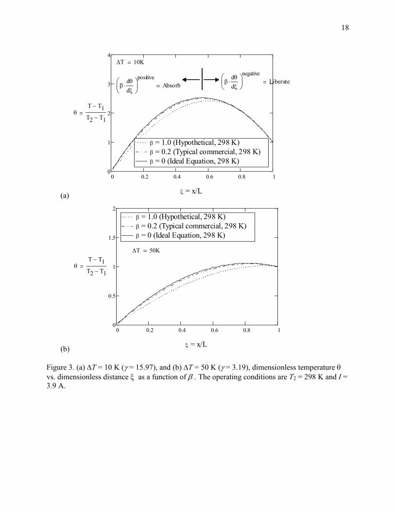
Figures 3 (a) and (b) show the temperature distributions at T2 = 298 K and I = 3.9 A as a
function of for T = 10 K ( = 15.97) and T = 50 K ( = 3.19). In Figure 3 (a), the Joule
heating appears dominant with a high value of = 15.97, while in Figure 3 (b) the thermal
conduction is approximately balanced with the Joule heating with a low value of = 3.19. For
the commercial cases in the both figures with = 0.2, the Thomson effects appear small
compared to the ideal equation at = 0. The hypothetical cases at = 1.0 obviously provide
salient examples for the Thomson effect. Since the temperature gradient at = 0 counteracts the
Peltier cooling, the slightly lower temperature distribution near zero acts as improving the net
cooling power. The Thomson heat is effectively described by the product of and dd . The
Thomson heat acts as absorbing heat when the dd is positive, while it acts as liberating
heat when the dd is negative, which are shown in Figure 3 (a). In the first half of the
temperature distribution, both and dd are positive, so that the product is positive. It is
known that the moving charged electrons or holes (see Figure 1) transport not only the electric
energy but also the thermal energy as absorbing and liberating depending on the sign of dd
along the thermoelement. The temperature distribution is slightly shifted to the right giving the
lower temperature distribution near = 0, which results in the improved cooling power at the
cold junction. It is interesting to note that the product of the current I and the Seebeck coefficient
in Equation (37) is always positive, therefore making no contribution to the final sign of the
Thomson heat. If the current is positive in a p-type element, the sign of is positive. If the
current is negative in a n-type element, the sign of is negative (see Figure 1). Therefore, the
product is always positive.
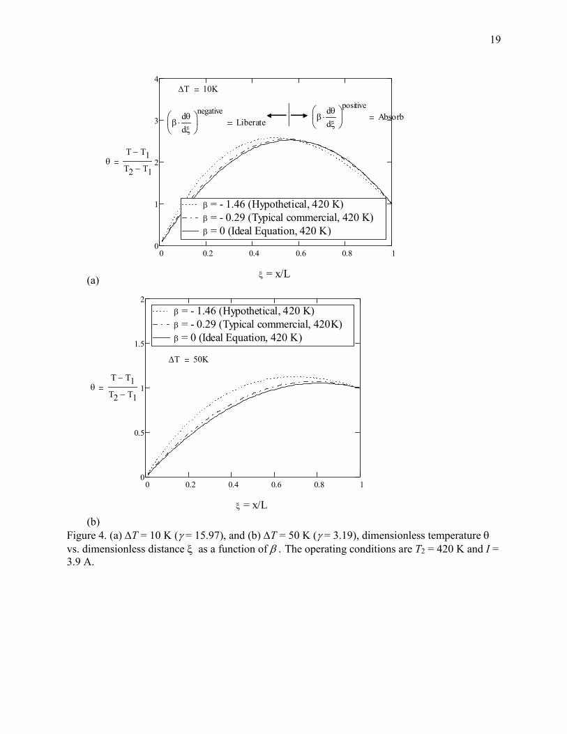
Now consider the linear curve fit of the second part (for the range from 350 K to 450 K) of
the temperature-dependent Seebeck coefficient in Figure 2, where the in Equation (37) is
negative. Figures 4 (a) and (b) show the temperature distributions at T2 = 420 K and I = 3.9 A as
a function of for T = 10 K ( = 15.97) and T = 50 K ( = 3.19). For the commercial cases at
= - 0.29 in the both figures, the Thomson effect again appears small compared to the ideal
equation at = 0. The hypothetical cases at = - 1.46 obviously provide salient examples for the
Thomson effect. Note that the temperature distribution is slightly shifted to the left giving the
higher temperature gradient near = 0, which results in the reduced cooling power at the cold
junction. This is opposite of the cases at T2 = 298 K shown in Figure 3 (a) and (b). In Figure 4 (a),
it is seen that the first and second half segments of the thermoelement exhibit the heat liberation
and absorption, while the moving charged carriers (electrons or holes) are moving from left to
right. Actually the moving carriers are resultantly at a speed from left to right, while numerous
carriers are still moving in random directions, which can transport the thermal energy from right
to left without problems.
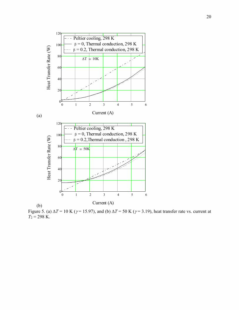
Equation (41) represents the net cooling power which is calculated by subtracting the
thermal conduction from the Peltier cooling. Each term of the equation is separately presented in
Figures 5 (a) and (b) in order to examine the fraction of the thermal conduction to the Peltier
cooling as well as the Thomson effect in terms of the heat transfer rate. In Figure 5 (a) for T =
10 K, the percentage of the thermal conduction to the Peltier cooling at I = 3.9 A is 46.2%, while,
in Figure 5 (b) for T = 50 K, the percentage is 81.6%. This indicates that the significant portion
of heat generated by the Peltier cooling is wasted surprisingly by the thermal conduction and this
waste robustly increases as T increases. Note that the net cooling power is zero at I = 1.5 A. No
14
gain in the cooling power is seen until after I = 1.5 A. It would be desirable from the above
cognition to develop a thermoelectric material that has a low thermal conductivity to minimize
the waste heat by the thermal conduction. However, lowering the thermal conductivity without
affecting the electrical conductivity is challenging according to the Wiedemann-Franz law.
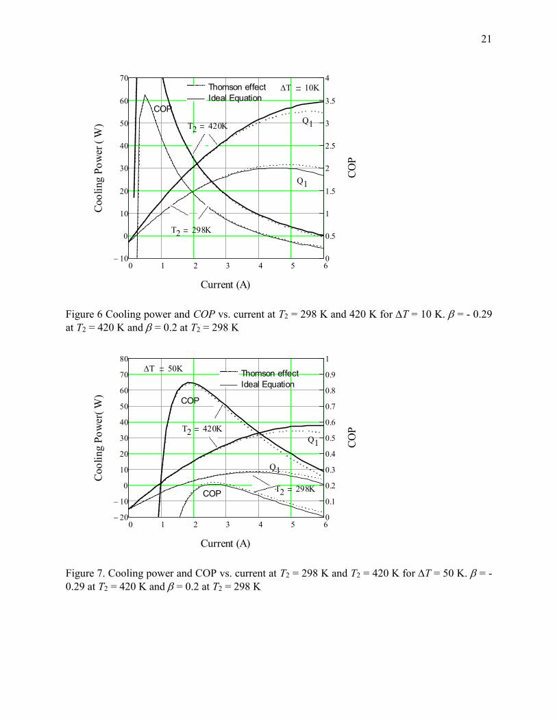
The net cooling power 1Q in Equation (41) and the coefficient of performance (COP) in
Equation (46) along the current at both T2 = 298 K (thin lines) and 420 K (thick lines) for T =
10 K are presented in Figure 6. The maximum current for this commercial module is 3.9 A as
shown in Table 1, so the operating current barely exceeds the maximum current in practice. The
slight improvement by the Thomson effect on 1Q at 298K is also reflected on the corresponding
COP wherein the effect appears even smaller. Of interest is that 1Q at T2 = 420 K makes in the
opposite way. The Thomson effect improves 1Q at 298 K while it deteriorates 1Q at 420 K.
As T increases, the both cooling power and COP decrease, which is shown in Figure 7.
There is no appreciable change on the Thomson effect with increasing T.
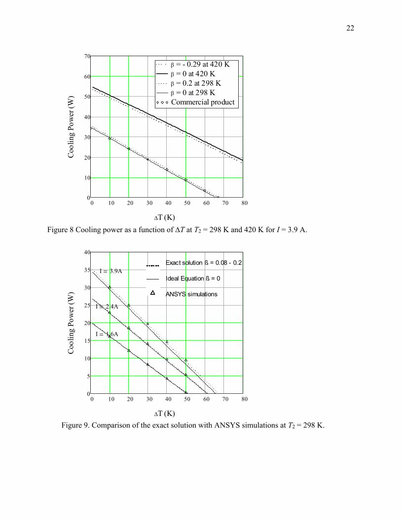
The net cooling powers at T2 = 298 K and 420 K as a function of T are presented in Figure
8. At a glance the exact solutions ( ≠ 0) and the ideal equation ( = 0) are very close to each
other. Furthermore, the two at 298 K are in good agreement with the available data of
commercial products which are usually empirical data. It should be pointed out that the gaps
between the Thomson effect and the ideal equation at both T2 = 298 K and 420 K remain
unchanged, which is interpreted to be good for the predictability by the ideal equation. It is
postulated that the ideal equation is very effective for prediction of the performance of
thermoelectric coolers, if the averaged Seebeck coefficient is used.
In order to elucidate the agreement between the exact solutions, the ideal equation, and the
numerical simulations, the numerical software ANSYS was deployed with the exactly same
material properties, dimensions, and boundary conditions as those imposed on the exact solutions.
Recall that the exact solutions were analytically obtained using mathematical software Mathcad.
The exact solutions with Equations (36) and (42) and the methodology used are justified by
comparing them with the ANSYS simulations as shown in Figure 9. The ANSYS solves
numerically the governing equations of Equations (17), (20), (22), and (30) by means of the
finite element method with the given boundary conditions [17]. It is found in Figure 9 that the
exact solutions are in precise agreement with the ANSYS simulations. Accordingly, the gaps
between the exact solutions and the ideal equation implicate the quantities associated with the
assumption made in the ideal equation. It is also deduced that the assumption of the negligible
Thomson coefficient is indeed appropriate for either the moderate currents or the moderate
temperature differences. However, the errors between the ideal equation and the exact solutions
could reach up to 8% for the maximum current (here I = 3.9 A) and the high temperature
difference (T = 50 K). All the procedures and conditions implemented in the exact solutions
and the ideal equation turned out to be correct.
15
4. Conclusions
A positive Thomson coefficient improves the performance of a thermoelectric cooler while a
negative Thomson coefficient reduces the performance.
A substantial amount of heat absorbed by the Peltier cooling is wasted by the thermal
conduction, substantially increasing with increasing the temperature difference.
The exact solutions of the analytical differential equations including the Thomson effect are
in excellent agreement with the ANSYS numerical simulations.
The ideal equation effectively predicts the performances of thermoelectric coolers if the
Seebeck coefficient is correctly evaluated at the average temperature of the low and high
junction temperatures.
References
[1] Peltier J.C., New experiments on the calorific electric currents (Nouvelle experiences sur la
caloricite des courans electrique ), Ann. Chim.LV1 371, 1834
[2] Thomson W., Account of researchers in thermo-electricity, Philos. Mag. [4], 8, 62, 1854.
[3] Onsager L., Reciprocal Relations in Irreversible Processes. I., Phys. Rev., 37, 405-526, 1931.
[4] Callen H.B., The application of Onsager’s reciprocal relations to thermoelectric,
thermomagnetic, and galvanomagnetic effects, Phys. Rev., 73, 1349-1358, 1948
[5] Casimir H.B.G., On Onsager’s principle of microscopic reversibility, Reviews of Modern
Physics, 17, 343-350, 1945
[6] Verhas J., Onsager’s reciprocal relations and some basic laws, Journal of Computational and
Applied Mechcanics, Vol. 5, No.1 157-163, 2004
[7] Landau L.D., Lifshitz E.M., Elecrodynamics of continuous media, Pergamon Press, Oxford,
UK, 1960.
[8] Ioffe A.F., Semiconductor thermoelements and thermoelectric cooling, Infoserch Limited,
London, UK, 1957.
[9] Rowe D.M., CRC Handbook of Thermoelectrics, CRC Press, Boca Raton, FL, USA, 1995.
[10] Lee H.S., Thermal design: heat sinks, thermoelectrics, heat pipes, compact heat exchangers,
and solar cells, John Wiley & Sons, Inc., Hoboken, New Jersey, USA, 2010.
[11] Chen J., Yan Z., The influence of Thomson effect on the maximum power output and
maximum efficiency of a thermoelectric generator, J. Appl. Phys., 79, 8823-8828, 1996
[12] Huang M.J., Yen R.H., Wang A.B., The influence of the Thomson effect on the
performance of a thermoelectric cooler, Int. J. Heat Mass Trans, 48, 413-418, 2005
[13] Du C.Y., Wen C.D., Experimental investigation and numerical analysis for one-stage
thermoelectric cooler considering Thomson effect, Int. J. Heat Mass Transfer, 54: 4875-4884,
2011.
[14] Chen W.H., Liao C.Y., Hung C.I., A numerical study on the performance of miniature
thermoelectric cooler affected by Thomson effect, Applied Energy, 89: 464-373, 2012.
[15] Goldsmid H.J., Introduction to thermoelectricity, Spriner, Heidelberg, Germany, 2010.
[16] Nolas G.S., Sharp J., Goldsmid H.J., Thermoelectrics, Springer, Heidelberg, Germany, 2001.
[17] Antonova E.E., Looman D.C., Finite elements for thermoelectric device analysis in ANSYS,
24th International Conference on Thermoelectrics, 215-218, 2005.
[18] Min G., Rowe D.M., Kontostavlakis K., Thermoelectric figure-of-merit under large
temperature differences, J. Phys. D; Appl. Phys., 37, 1301-1304, 2004.
[19] Yamashita O., Resultant Seebeck coefficient formulated by combining the Thomson effect
16
with the intrinsic Seebeck coefficient of a thermoelectric element, Energy Conversion and
Management, 50, 2394-2399, 2009.
[20] Yamashita O., Effect of temperature dependence of electrical resistivity on the cooling
performance of a single thermoelectric element, Applied Energy, 85, 1002-1014, 2008.
[21] Sandoz-Rosado E.J., Weinstein S.J., Stevens R. J., On the Thomson effect in thermoelectric
power devices, International Journal of Thermal Sciences,66, 1-7,2013,.
17
Figure 1. Thermoelectric cooler with p-type and n-type thermoelements.
200 250 300 350 400 450 500140
160
180
200
Intrinsic material properties
Linear curve fit
Linear curve fit
Curve fit
Temperature (K)
V
K
Figure 2. Seebeck coefficient as a function of temperature for Laird products.
18
(a)
0 0.2 0.4 0.6 0.8 10
1
2
3
4
= 1.0 (Hypothetical, 298 K)
= 0.2 (Typical commercial, 298 K)
= 0 (Ideal Equation, 298 K)
= x/L
T 10K
d
d
negative
Liberate
d
d
positive
Absorb
T T1
T2 T1
(b)
0 0.2 0.4 0.6 0.8 10
0.5
1
1.5
2
= 1.0 (Hypothetical, 298 K)
= 0.2 (Typical commercial, 298 K)
= 0 (Ideal Equation, 298 K)
= x/L
T 50K
T T1
T2 T1
Figure 3. (a) T = 10 K ( = 15.97), and (b) T = 50 K ( = 3.19), dimensionless temperature
vs. dimensionless distance as a function ofThe operating conditions are T2 = 298 K and I =
3.9 A.
19
(a)
0 0.2 0.4 0.6 0.8 10
1
2
3
4
= - 1.46 (Hypothetical, 420 K)
= - 0.29 (Typical commercial, 420 K)
= 0 (Ideal Equation, 420 K)
= x/L
T 10K
d
d
positive
Absorb
d
d
negative
Liberate
T T1
T2 T1
0 0.2 0.4 0.6 0.8 10
0.5
1
1.5
2
= - 1.46 (Hypothetical, 420 K)
= - 0.29 (Typical commercial, 420K)
= 0 (Ideal Equation, 420 K)
= x/L
T 50K
T T1
T2 T1
(b)
Figure 4. (a) T = 10 K ( = 15.97), and (b) T = 50 K ( = 3.19), dimensionless temperature
vs. dimensionless distance as a function ofThe operating conditions are T2 = 420 K and I =
3.9 A.
20
(a)
0 1 2 3 4 5 60
20
40
60
80
100
120
Peltier cooling, 298 K
= 0, Thermal conduction, 298 K
= 0.2, Thermal conduction, 298 K
Current (A)
Hea
t T
ransf
er
Rat
e (W
)
T 10K
(b)
0 1 2 3 4 5 60
20
40
60
80
100
120
Peltier cooling, 298 K
= 0, Thermal conduction, 298 K
= 0.2,Thermal conduction , 298 K
Current (A)
Hea
t T
ransf
er
Rat
e (W
)
T 50K
Figure 5. (a) T = 10 K ( = 15.97), and (b) T = 50 K ( = 3.19), heat transfer rate vs. current at
T2 = 298 K.
21
0 1 2 3 4 5 610
0
10
20
30
40
50
60
70
0
0.5
1
1.5
2
2.5
3
3.5
4
Current (A)
Co
oli
ng
Po
wer
( W
)
CO
P
Thomson effect T 10K
Ideal Equation
COP
Q1T2 420K
Q1
T2 298K
Figure 6 Cooling power and COP vs. current at T2 = 298 K and 420 K for T = 10 K. = - 0.29
at T2 = 420 K and = 0.2 at T2 = 298 K
0 1 2 3 4 5 620
10
0
10
20
30
40
50
60
70
80
0
0.1
0.2
0.3
0.4
0.5
0.6
0.7
0.8
0.9
1
Current (A)
Co
oli
ng
Po
wer
( W
)
CO
P
T 50KThomson effect
Ideal Equation
COP
T2 420K
Q1
Q1
T2 298KCOP
Figure 7. Cooling power and COP vs. current at T2 = 298 K and T2 = 420 K for T = 50 K. = -
0.29 at T2 = 420 K and = 0.2 at T2 = 298 K
22
0 10 20 30 40 50 60 70 800
10
20
30
40
50
60
70
= - 0.29 at 420 K
= 0 at 420 K
= 0.2 at 298 K
= 0 at 298 K
Commercial product
T (K)
Coo
ling P
ow
er (
W)
Figure 8 Cooling power as a function of T at T2 = 298 K and 420 K for I = 3.9 A.
0 10 20 30 40 50 60 70 800
5
10
15
20
25
30
35
40
T (K)
Coo
ling P
ow
er (
W)
Exact solution ß = 0.08 - 0.2
I 3.9A
Ideal Equation ß = 0
ANSYS simulations
I 2.4A
I 1.6A
Figure 9. Comparison of the exact solution with ANSYS simulations at T2 = 298 K.
Recommended