MarkusSchmid
TireModelingforMultibodyDynamicsApplications
Simulation‐BasedEngineeringLaboratory
UniversityofWisconsin‐Madison
2011


i
Abstract
Invehicledynamics,tiresareoneofthemostimportantfactorsthatgovernthebehaviorofa
movingvehicle.Theyaretheonlylinkbetweenthevehiclechassisandtheroadandhaveto
transmitvertical,longitudinalandlateralforces.Inordertobeabletodescribeavehicle’s
movementproperly,itisnecessarytounderstandthetires’characteristicsandtheireffecton
certaindrivingsituations.
Whileempiricaldatagainedfromon‐the‐roaddrivingexperimentswithrealtiresis
obviouslythemostaccurate(giventhatconditionsaresimilartothedesiredsimulation),thereare
reasonstochoosedynamicalsimulationsinstead.Sinceproductcyclesanddevelopmenttimesare
continuouslyreducedduetocompetitionandprogressoftechnology,buildingphysicalprototypes
inanearlystageofdevelopmentistime‐consumingandveryexpensive.Furthermore,ifthedesign
ischanged,theprototypehastobeupdatedagainandagain.Clearly,withlargermachinerylike
constructionvehicles,thisbecomestimeandcostprohibitive.Thustendingtowardssimulationsin
earlydevelopmentstagescanbehighlybeneficialtothefinaldesign.
Tiresareverycomplexproductsandnottrivialtodescribe.Theircharacteristicsare
influencedbyseveralfactorslikedesignofthetireitself(e.g.material,treadpattern,carcass
stiffness),airpressureinsidethetireandtextureoftheroadsurface,tonameafew.
Severalmodelingapproacheshavebeendevelopedtodescribethephysicsoftiressothat
theycanbeanalyzedandevaluatedmathematically.Inthefirstpartofthiswork,acombinationof
thesteady‐stateMagicFormulaapproach(describedin[1],[2]and[3])andtheSingleContactPoint
transienttiremodel[3]isusedtoimplementatiremodelthatcanhandletranisentdriving
situationsintothemultibodydynamicsengineChrono::Engine[4].Forvalidationandexperimental
purposes,thetiremodelisthenintegratedwithavehiclemodelanddifferentdrivingsituationsare
analyzed.Thesecondpartofthisresearchintroducesabeamelementtypephysicalmodelthat
permitsinteractionwithflexibleterrainforoff‐roadapplications.
ii
Acknowledgements
Firstofall,IwouldliketogreatlythankmyadvisorattheDepartmentofMechanical
Engineering,ProfessorDanNegrut,forallthesupport,thevaluableadviceandneverrunningoutof
M&M’stokeepupthemotivation.ThankyouDanformakingmepartoftheteam!
Also,thankyouverymuchtoallthepeopleattheSimulation‐BasedEngineeringLaboratory
(SBEL)forthegreatatmosphereinthelab,helpingoutwheneverpossibleandmakingthisagreat
year!
Finally,IwouldliketothanktheGermanAcademicExchangeService(DAAD),theInstitute
forMachineTools(IfW)attheUniversityofStuttgartandtheDepartmentofMechanical
EngineeringattheUniversityofWisconsin‐MadisonformakingmystudiesintheUnitedStatesand
thereforethisworkpossible.

iii

iv
TableofContents
Abstract.......................................................................................................................................................................i
Acknowledgements...............................................................................................................................................ii
TableofContents..................................................................................................................................................iv
ListofFigures.........................................................................................................................................................vi
1 Introduction....................................................................................................................................................1
1.1 TireDynamics.........................................................................................................................................................1
1.1.1 TireForcesandTorques...........................................................................................................................1
1.1.2 LongitudinalandLateralSlip..................................................................................................................2
1.1.3 TurnSpin.........................................................................................................................................................3
1.2 TireModeling..........................................................................................................................................................5
1.2.1 TheMagicFormulaTireModel..............................................................................................................5
1.2.2 TheSingleContactPointTransientTireModel...............................................................................8
2 ImplementationoftheMagicFormulaTireModel.........................................................................14
2.1 MATLABimplementation................................................................................................................................14
2.1.1 Tirepropertyfile(*.tire)........................................................................................................................15
2.1.2 Transienttiremodel................................................................................................................................16
2.1.3 MagicFormulasteady‐statemodel....................................................................................................16
2.1.4 Modelverification.....................................................................................................................................18
2.2 Chrono::Engineimplementation..................................................................................................................24
2.2.1 ThemultibodydynamicssimulationengineChrono::Engine.................................................24

v
2.2.2 TranslationoftheMATLABimplementationtoC++..................................................................24
2.2.3 VehicleandtiremodelusedinChrono::Engine...........................................................................25
2.2.4 TheStandardTyreInterface(STI).....................................................................................................26
2.2.5 OrganizationoftheMagicFormulatiremodelinChrono::Engine.......................................28
2.2.6 Obtainingreal‐timevehicledata.........................................................................................................29
2.2.7 Applicationoftheforcesandmomentstothevehiclemodel.................................................31
2.2.8 Resultsandconclusions.........................................................................................................................32
3 Beamtiremodelforinteractionwithdeformableterrain...........................................................35
3.1 Tiretreadmodel..................................................................................................................................................35
3.2 Forcesinthetiretreadandcontactpatch................................................................................................37
3.3 Modelverification...............................................................................................................................................41
3.3.1 Verticalmotionofthewheel................................................................................................................42
3.3.2 Longitudinalmotionofthewheel......................................................................................................44
3.4 Resultsandfuturework...................................................................................................................................50
4 Summary........................................................................................................................................................51
5 References.....................................................................................................................................................52
A Appendix........................................................................................................................................................54
A.1 MagicFormulaequationsandfactors[3].................................................................................................54
A.2 .tirepropertyfileusedintheMagicFormulaimplementations.....................................................62

vi
ListofFigures
Fig.1.1:Signconventionandtirereferenceframe[3]..............................................................................................1
Fig.1.2:Rotationalslipresultingfrompathcurvatureandwheelcamber[3]..............................................4
Fig.1.3:Thetireasanonlinearfunctionwithmultipleinputsandoutputs(steady‐state)[8]...............5
Fig.1.4:MagicFormulafactors[9]....................................................................................................................................7
Fig.1.5:Sideforcecharacteristicsofa315/80R22.5trucktireforvaryingnormalloads.Comparison
ofMagicFormulacomputedresultswithmeasureddata[3].................................................................................8
Fig.1.6:SingleContactPointTireModel(topview)[3]...........................................................................................9
Fig.1.7:EffectiverollingradiusanddefinitionofslippointS[7].....................................................................10
Fig.1.8:Proceduretocalculateforceandmomentvariationsatthecontactpatch.................................13
Fig.2.1:FlowchartshowingtheconnectionofthetransientmodelandtheMagicFormulamodelin
theMATLABimplementation...........................................................................................................................................15
Fig.2.2:SubroutinesusedintheMATLABimplementationofthetransientmodelandtheMagic
Formula......................................................................................................................................................................................17
Fig.2.3:VelocityprofilesfortestingscenarioA........................................................................................................18
Fig.2.4:TransientslipquantitiesforscenarioA......................................................................................................19
Fig.2.5:LongitudinalforceforscenarioA...................................................................................................................20
Fig.2.6:RollingresistancemomentforscenarioA..................................................................................................20
Fig.2.7:SideslipangleandlateralslipvelocityforscenarioB..........................................................................21
Fig.2.8:TransientslipquantitiesforscenarioB.......................................................................................................22
Fig.2.9:LongitudinalforceforscenarioB...................................................................................................................22
Fig.2.10:LateralforceforscenarioB............................................................................................................................23
Fig.2.11:VisualizationofthevehiclemodelusedinChrono::Engineasspecifiedin
demo_suspension.cpp(modified)...................................................................................................................................25
Fig.2.12:SchematicviewoftheSTI[8]........................................................................................................................27

vii
Fig.2.13:Vectorsusedtodescribethemovementofthevehicle......................................................................29
Fig.2.14:CodesnippetofthegetVehicleData()subroutine......................................................................30
Fig.2.15:Longitudinalvelocitiesfortheleftreartire............................................................................................32
Fig.2.16:Longitudinalslipandlongitudinalforcefortheleftreartire..........................................................32
Fig.2.17:Sideslipangleandlateralslipvelocityfortheleftfronttire...........................................................33
Fig.2.18:Transientslipangleandlateralforcefortheleftfronttire..............................................................33
Fig.3.1:Beamelementsetupforthetiretread:anetofbeamsconnectedtotherim..............................36
Fig.3.2:Circumferentialandradialforcesatelement(i,j)...................................................................................37
Fig.3.3:Setofforcesactingononeelement(i,j).......................................................................................................38
Fig.3.4:Deflectedtireandresultingnormalforcesduetocontactwithground........................................42
Fig.3.5:Deflectedtireandresultingnormalforcesduetocontactwithground........................................43
Fig.3.6:ResultingverticalForcedevelopedinthetirecontactpatch.............................................................43
Fig.3.7:Verticalmovementofthewheelhubcenter(integrationstepsize:0.001s)...............................44
Fig.3.8:Kinematic‐basedfrictionmodel[17]...........................................................................................................45
Fig.3.9:ScenarioA:angularposition,velocityandaccelerationofthewheel.............................................47
Fig.3.10:Slipandtotallongitudinalforce...................................................................................................................48
Fig.3.11:ScenarioB:xvelocityandaccelerationofthewheelcenter............................................................49
Fig.3.12:ScenarioB:Slipandtotallongitudinalforce...........................................................................................50
Fig.A.5.1:Positivedirectionsofforcesandmoments[3]....................................................................................56


1 Int
B
Chrono:
theMagi
1.1 Ti
T
Thesequ
1.1.1 T
T
Thisisfo
adapted
troductio
Beforeweco
:Engine,we
icFormulam
ireDynam
Themostim
uantitiesallo
TireForce
Thecoordina
orpracticalr
versionoft
on
onsiderthei
needtocov
modelandth
mics
mportantfact
owustodes
sandTorq
ateframean
reasons,sin
theSAEstan
Fig.1
implementa
erthebasic
hesinglecon
torsintired
scribethech
ques
ndsignconv
cethetirem
ndardcoordi
1.1:Signconv
1
tionoftheM
ideasoftire
ntactpointt
dynamicsare
haracteristic
ventionused
modelsprop
inateframe
ventionandti
MagicFormu
edynamicsa
transientmo
etireforces
csofatirein
dinthiswor
osedin[3]a
(SAEJ670e
irereference
ulatiremode
andtiremod
odel).
andtorques
nalldrivings
kisadopted
alsousethis
1976)andis
frame[3]
elinto
deling(inpa
s,slipandtu
situations.
dfromPacej
sasareferen
sshowninF
articular
urnspin.
ka[3].
nce.Itisan
Fig.1.1.

2
Inthisreferenceframe,
isthespeedoftravelofthewheelcenter.
isthesideslipangle(theanglebetweenthexz‐planeand ).
isthecamberangle(theanglebetweenthexz‐planeandthemeanwheelplane).
istheyawrateorturnslipvelocity.
isthelongitudinalforceactingalongthex‐axis( 0foracceleration, 0for
braking).
isthelateralorsideforce.Itisappliedatapointinadistance behindthecenter
ofthecontactzoneoftireandroad[5].
istheloadornormalforce.
istheself‐aligningtorque.Itiscausedbythenon‐centralapplicationof and
forcesthemeanplaneofthewheeltowardsthedirectionof . canbecalculated
as ∗ ,wheretisthepneumatictrail[5].
Ingeneral, , and arefunctionsoflongitudinalslip ,load ,sideslipangle and
camberangle [3].
1.1.2 LongitudinalandLateralSlip
Unlessthewheelisrollingfreely(withnodrivingorbrakingtorqueappliedand 0),
longitudinalandlateralslipquantitieshavetobeconsidered.Morespecific,atireneedsslip(dueto
elasticdeformationsorsliding)totransmitforces[6].

3
Ingeneral,whenatorqueisappliedtothewheel,wehavetodistinguishtheactualforward
speedofthetireovertheroadsurface(x‐componentofthespeedoftravel: )andthevelocity
thatisclassifiedbythetire’sangularvelocityΩanditseffectiverollingradius [3]:
x0 Ω eV r (1.1)
Toquantifythedifferenceof and ,longitudinalslip isdefinedas[3]:
x0 Ω x x e
x x
V V V r
V V
(1.2)
Thisresultsinnegative forbrakingandpositive foracceleration(positivelongitudinal
slipmeanspositivelongitudinalforce ).
Bythesametoken,lateralorsideslip iscalculatedfromtheratioofthelateralvelocity
andtheforwardvelocity ofthewheel:
tan y
x
V
V (1.3)
Again,positivesideslip meanspositivesideforce .Theslipangle denotestheangle
betweenthetravellingdirectionandtherollingdirectionofthetire.
1.1.3 TurnSpin
Theyawvelocity(orturnslipvelocity)ΨdisplayedinFig.1.2denotestheangularvelocityof
thewheelaboutthenormaltotheroad[7].

I
canbed
where
axleand
T
Inthisconte
escribedas
∗ istheforw
dlocatedatd
Turnslip
t
Fig.1.2
ext,spinslip
afunctiono
*z
cxV
wardrunnin
distance fr
(thatis,spin
*
1
cxV R
2:Rotationals
(thecomp
ofyawratea
*
sin
cxV
ngspeedoft
romthewhe
nonlydueto
1
R
4
slipresultingwheelcambe
ponent
andcambera
,
theimaginar
eelcenterbe
opathcurva
frompathcuer[3]
oftheabsol
angle:
rypoint ∗t
elowroadle
ature,notwh
urvatureand
utespeedof
hatisperpe
evel[3].
heelcamber
frotationve
endiculartot
r )isdefine
ector )
(1.4)
thewheel
edas:
(1.5)

1.2 Ti
M
quantitie
shownin
T
statecon
Formula
1.2.1 T
O
propose
compare
formulas
ireModel
Mostgenera
es,anglesan
nFig.1.3.
Fig.1.3
Todescribet
nditions,sev
aTireModel
TheMagic
Ofthemany
din[1],[2]
edtoexperim
saren’tderi
ling
al,atirecanb
ndloadforce
3:Thetireas
the“blackb
veralapproa
.
FormulaT
differenttir
and[3]ison
mentaldata
ivedfromap
bemodeled
e)andoutpu
anonlinearf
ox”between
acheshaveb
TireModel
remodelsth
neofthemo
.Theapproa
physicalbac
5
asanonline
uts(longitud
functionwith
state)[8
ninputsand
beensuggest
l
hatareavaila
ostadvanced
achofthem
ckgroundtha
earsystemw
dinalandlat
multipleinp]
doutputsfor
ted,includin
abletoday,t
dandhaspr
modelissemi
atmodelsth
withmultipl
teralforcesa
utsandoutpu
rsteady‐stat
ngPacejka’s
theMagicFo
roventobev
i‐empirical,m
hetire’sstru
einputs(sli
andtiremom
uts(steady‐
teandnons
so‐calledM
ormulaTire
veryaccurat
meaningtha
ucturebutra
p
ments),as
teady‐
Magic
Model
tewhen
atthe
atherare

6
mathematicalapproximationsofcurvesthatwererecordedinexperiments.Forthispurpose,
scalingfactorshavetobeobtainedfrommeasurements.
ThegeneralformoftheMagicFormulais[3]:
sin[ arctan arctan( ) ]y D C Bx E Bx Bx , (1.6)
whereyrepresentsatireforceortorqueandxistheslipquantitythisforceortorquedependson
(i.e.longitudinalorlateralslip).B,C,D,Earefactorstodefinethecurve’sshapeinordertogetan
appearancesimilartotherecordedcurve.Specifically,
B isastiffnessfactor
C isashapefactor
D isthepeakvalue
E isacurvaturefactor
arctan istheslopeofthecurveattheorigin.
Eachofthesefactorshastobeapproximatedfrommeasureddatafromexperimentsforthe
respectivetireandenvironment.Itisalsopossibletoapplyanoffsetin x and y withrespecttothe
origintothisgeneralformula.Anoffsetcanariseduetoply‐steerandconicityeffectsaswellas
wheelcamber[3].Theshiftin x and y canbeperformedbyusingthemodifiedcoordinates
VY X y x S with beingtheverticalshiftand
Hx X S with beingthehorizontalshift.

F
A
thosepa
describe
torque),
A
where
T
showscu
Fig.1.4show
Asinputvari
arametersal
edbythefor
depending
Asanexamp
yoF
istheslip
Todisplayth
urvesobtain
wsaninterpr
iable wec
sodependo
rmulamight
ontheprobl
ple,thesidef
sin[y yD C
angle.Thef
heagreemen
nedfromme
retationoft
Fig.1.4:
canusetan
onverticallo
be (longi
lem.
force can
arctany yB
fullsetoffac
ntoftheMag
easurements
7
thefactorsu
MagicFormu
( beingth
oad andca
itudinalforc
nbedescrib
(y y yE B
ctorsinvolve
gicFormula
scompared
sedinthege
ulafactors[9]
helateralslip
amberangle
ce), (sidef
bedas[3]:
arctan(y B
edcanbefou
approachan
toMagicFor
eneralform
]
pangle)orκ
e .Theoutp
force)or
))]y y VB S
undinAppe
ndexperime
rmulacomp
oftheMagic
κ(longitudin
putvariable
(selfalignin
Vy ,
ndixA.1.
entaldata,F
putedresults
cFormula.
nalslip)–
ng
(1.7)
Fig.1.5
s.

H
e.g.pure
describe
theMagi
imperfec
wellasd
T
consider
1.2.2 T
U
transien
Fig.1.loads
However,th
ecorneringo
ethenon‐lin
icFormulai
ctions,off‐ro
dealingwith
Todescribe
redinadditi
TheSingle
UnliketheM
nttiremodel
5:Sideforces.Comparison
eMagicForm
orbrakingo
near,nonste
sincapable
oadusageof
non‐flatroa
non‐linear,n
ion.
eContactP
MagicFormu
lpresentedi
characteristicnofMagicFo
mulamodel
racombina
eady‐statedr
ofdescribin
fthetire(inc
adcondition
nonsteady‐
ointTrans
laTireMode
in[3]iscapa
8
csofa315/8ormulacompu
itselfislimi
ationofthose
rivingsituat
ngthermalef
cludinginte
ns(shortwav
statedriving
sientTireM
elalone,the
ableofdescr
0R22.5truckutedresultsw
itedto(quas
etwo[2],an
tionsthatare
ffects,tirew
ractionwith
velengths).
gsituations,
Model
esemi‐non‐li
ribingnon‐l
ktireforvarywithmeasure
si)steady‐st
ndistherefo
eofinterest
wearanddur
hflexibleter
,asecondap
inearSingle
inear,nonst
yingnormalddata[3]
tateconditio
orenotsuffic
tinthiswork
rability,tire
rrain,cf.chap
pproachhas
ContactPoi
teady‐state
onsonly,
cientto
k.Also,
pter3)as
tobe
int
driving

situation
[10],the
T
contactp
springs(
groundi
groundg
slipdata
currentt
F
by and
andco
nswhencom
emodelislim
Thebasicide
point that
(representin
inbothlong
generateslo
acanthenbe
transientfor
Figure1.6sh
d duetoth
ontactpatch
mbinedwith
mitedtolow
eaofthemo
tisconnecte
ngtheflexib
itudinaland
ongitudinala
eputintoth
rceandtorq
Fig.1
howstheset
hedifferentv
hspeed ′ r
thesteady‐
wslippages(
odelistocon
edtothewh
ilityofthec
dlateraldire
andsideforc
esteady‐sta
quevariation
.6:SingleCon
tupofthem
velocitiesof
respectively
9
stateMagic
(excludinge
ncentratethe
heelrimwith
carcass)allow
ection.Thus
ceaswellas
ateMagicFo
ns[3].
ntactPointTi
odelfromth
slippoint
y).
Formulaeq
.g.ABSbrak
einteraction
hlongitudina
wthecontac
theslipofth
self‐alignin
rmulamode
reModel(top
hetopview.
andsinglec
uations.How
king).
nofroadand
alandlatera
ctpointtosl
hecontactp
ngtorque.Lo
eldescribed
pview)[3]
Thecarcass
contactpoin
wever,assh
dtireinasi
alsprings.Th
lipwithresp
pointrelative
ongitudinala
in1.2.1toc
sspringsare
nt ′(wheels
hownin
ngle
hese
pectto
eto
andlateral
calculate
edeflected
slipspeed

T
imaginar
istheeff
O
freely,i.e
direction
when m
I
displaye
T
compon
Todescribet
rypointisa
fectiverollin
Obviously,th
e.slipisnot
nwiththelo
movessidew
Inthefollow
ed.Theyhav
Thechangeo
entsofthev
du
dt
dv
dt
Fig.1.7:E
themotiono
ttachedtoth
ngradius t
heslippoint
equaltozer
ongitudinals
ways[7].
wing,theequ
vebeenderiv
oflongitudin
velocitiesof
'( sx sV V
'( sy sV V
ffectiverollin
of ′theslip
hewheelrim
thathasbee
tmovesrela
ro.Whenthe
slipvelocity
uationsforth
vedin[3].
nalandlater
S and 'S ,re
)sx
)sy
10
ngradiusand
ppoint isin
mperpendic
endefinedin
ativetothew
ewheelisbr
.Bythe
heSingleCo
raldeflection
espectively,
definitionof
ntroduceda
culartothew
n(1.1).
wheelaxisw
raked,forex
sametoken,
ntactPointt
ns and o
asfollows:
f slippointS[
sareferenc
wheelcenter
whenthewhe
xample, mo
,alateralsli
transienttir
overtimeisr
7]
e(Fig.1.7).
r,wherethe
eelisnotrol
ovesinafor
ipvelocity
remodelare
relatedtoth
This
edistance
lling
rward
arises
e
hexandy
(1.8)
(1.9)

11
Afterseveralconversions,weobtainthefollowingdifferentialequationthatdescribesthe
lateraldeflectionduetosideslip :
1x x sy
dvV v V V
dt
, (1.10)
where istherelaxationlengthforsideslip / ( isthecorneringstiffness, isthe
lateraltirestiffnessatroadlevel)and isthewheelslipangle /| |.
Similarly,weobtainthedifferentialequationthatdescribesthelongitudinaldeflection :
1x x sx
duV u V V
dt
, (1.11)
where / istherelaxationlengthforlongitudinalslip(with beingthelongitudinal
tirestiffnessatroadleveland beingthelongitudinalslipstiffness),and /| |isthe
longitudinalwheelslipratio.
Ifthewheelistiltedsothatthecamberangle 0,anadditionalsideforceapplies.Thisis
partlybecauseofwheelpathcurvature,butalsobecauseofthetransientsideslipangle thatis
developedimmediatelyandcausesadditionalcarcassdeflection .
Thedifferentialequationforthiscaseis:
1| |F
x xF
dv CV v V
dt C
(withsideslipkeptequaltozero) , (1.12)
where isthecamberstiffnessforsideforce.

12
Bythesametoken,regardingtotalspin (thatis,includingturnslipandcamber)yieldsthe
followingdifferentialequation:
1| |F
x xF
dv CV v V
dt C
, (1.13)
where isthespinstiffnessforsideforceandtotalspin isdefinedas( isareductionfactor):
1 1 sin
xV . (1.14)
Usingtheseequations,wearenowabletocalculatethetransientslipquantities , ′and ′
forthetire.First,thecontactpointdeflections and areobtainedbysolvingtheinitialvalue
problemdefinedbythedifferentialequations(1.10),(1.11),(1.12)and (1.13)andusing
velocitiesandtirestiffnessesasinput.Inasecondstep, , ′and ′canbecomputedusingthe
followingequations:
'v
(1.15)
'u
(1.16)
' F
F
C v
C
(1.17)
Withthetransientmodelequationsintroducedabove,itisnowpossibletocalculatefirstthe
transientslipquantitiesandthen,usingtheMagicFormulaequationsshowninappendixA.1,
transientforceandmomentvariationsatthecontactpatch.ThisprocedureisshowninFig.1.8.

13
Fig.1.8:Proceduretocalculateforceandmomentvariationsatthecontactpatch
', ', '
,u v

14
2 ImplementationoftheMagicFormulaTireModel
ThisresearchaimsforanimplementationoftheMagicFormulatiremodelintothe
multibodydynamicsengineChrono::Engine[4].However,fordebuggingandtestingpurposes,the
transienttiremodelandtheMagicFormulasteady‐statemodelareimplementedinMATLABfirst.
Thismakesiteasiertooptimizethestructureofthecodewhileatthesametimethetranslationto
C++(thelanguageinwhichChrono::Engineiswritten)isofreasonableeffort.Also,MATLABoffers
fairlygoodvisualizationtoevaluatemeasureddata.
2.1 MATLABimplementation
Theflowoftheforcesandmomentscalculationprocessperformedateachtimestepis
showninFig.2.1.Specialattentionwaspaidtoaclear,easytounderstandmodularstructure.Thisis
especiallyimportantbecauseofthecomplexityoftheMagicFormulamodelwiththeseveral
subroutinesandthelargeamountofparametersusedtocharacterizethetire.
Thevehiclemodelprovidesvelocities(suchas| |,thelongitudinalvelocityofthewheel
center),wheelspeedofrevolution ,sideslipangle ,camberangle andturnslipvelocityΨ.For
codetestingwithoutneedforanactualvehiclemodel,thosequantitiesareassumedtobegivenat
eachtimestepwhendifferenttestingmaneuversareexamined.

15
Fig.2.1:FlowchartshowingtheconnectionofthetransientmodelandtheMagicFormulamodelintheMATLABimplementation
2.1.1 Tirepropertyfile(*.tire)
Touseavailabletiredataspecifiedforthecommercialmultibodydynamicssimulation
softwareMSCADAMS,itwouldbeappreciatedtouseADAMS’*.tirtiredatafilestoinputtiredata.
However,therearesomecompatibilityissuesbetweenthe2006versionoftheMagicFormulaused
inthisworkandthe2002versionusedinADAMS.Forthisreason,anewyetsimilartireproperty
file(*.tire)isintroduced.Thisfilecontainsalltheinformationtofullycharacterizeaspecifictire
underspecificenvironmentalconditionsusingtheMagicFormulacoefficients.Asmentionedbefore,
thecoefficientscanbeobtainedthroughparameterfittingofmeasurementdata(usuallycarriedout
bythetiresupplier).
Transient tire model- Solve ODEs -
Velocities,
, , , MF parametersfor tire of interest
Magic Formula steady-state model
Transient slip quantities
VelocitiesMF parameters
', ', ', '
Transient tire forces and moments
, , , , ,x y z x y zF F F M M M
Time loopTire property file(.tire) Vehicle model

16
2.1.2 Transienttiremodel
Sincesolvingthedifferentialequationsofthetransientsinglecontactpointmodelrequires
initialvaluesfordeflections and ,initiallystartingfromstandstill(where 0)is
suggested.Inthefollowingtimesteps,thedeflectionsfromtheprevioustimestepareusedasinitial
values.Theinitialvalueproblemsaresolvednumericallyusinga4thorderRunge‐Kuttamethod.
Specialhandlingforverylowvelocities| | hasbeenimplementedtoavoidhigh
deflectionsthatarebeyondwhatisphysicallypossibleandintroducesomeartificialdampingto
reduceoscillationsthatwouldotherwisebeundamped[3].
2.1.3 MagicFormulasteady‐statemodel
IntheMATLABimplementation,thetransientmodelsubroutinecallstheMagicFormula
subroutine,usingthetransientslipquantitiesaswellasvelocitiesandMagicFormulaparametersas
input.TheMagicFormulasubroutineitselfconsistsofsubroutinesforcalculationofeachforceand
momentofinterest.Atfirst,longitudinalforce,lateralforceandself‐aligningmomentarecalculated
forpurelongitudinalandsideslipconditions,respectively.Thesequantitiesarethenusedto
calculatetheactualforcesandmomentsduetocombinedlongitudinalandsideslip.Adetailed
structureofsubroutinesandparametersinvolvedisshowninFig.2.2.

17
Fig.2.2:SubroutinesusedintheMATLABimplementationofthetransientmodelandtheMagicFormula.
readTIRE.m
tireData
alphaPrimegammaPrimekappaPrimephiPrimephi_t
tireDataV_cV_s
getRelaxationLengths.m
can turn slip phi_t
be neglected?no yes
zeta_i = 1(i = 0,…,8)zeta_i ≠ 1
longitudinalForcePure.m lateralForcePure.m aligningTorquePure.m
longitudinalForceCombined.m lateralForceCombined.m aligningTorqueCombined.m
overturningCouple.mrollingResistanceMoment.m
205_60_R15_91V_2-2bar.tire
turnSlip.m
normalLoad.m
F_z
F_y0
F_yF_x
F_x0 M_z0
magicFormula.m
transientMF.m

2.1.4 M
A
andtoid
I
accelera
I
reaches
resulting
Thelong
Modelveri
Asetoftesti
dentifytheir
InscenarioA
ateandbrake
Inthisscena
avelocityof
gfromwhee
gitudinalslip
ification
ngscenario
rlimits.The
A,apurelylo
einastraigh
F
ario,aftersta
fabout
elspeedofre
pvelocity
s,AandB,h
tiretypeuse
ongitudinalm
htline(cf.Fi
ig.2.3:Veloci
artingfroms
13.3 att
evolutionΩ
isthediffe
18
havebeenca
edhereis20
maneuveris
ig.2.3).
ityprofilesfo
standstill,th
=9s.Dueto
andeffectiv
erenceoftho
arriedoutto
05/60R159
sexaminedw
rtestingscen
hevehicleac
oincreasing
verollingrad
osevelocitie
verifytheim
91V.
wherethev
narioA
cceleratesco
longitudinal
dius ishig
s:
mplemented
ehicleisass
onstantlyun
lslip,theve
gher(about1
Ω .
dmodels
umedto
ntilit
elocity
14.6 ).

W
isthenr
asbrake
t=19.9s
F
modelin
builtup
brakesli
T
thisman
braking
appliedf
Whilemaint
ollingfreely
eslipincreas
s.
Figure2.4sh
nconjunctio
whenstarti
ipisdevelop
Theresulting
neuveraresh
theforcetur
for 0.
tainingavelo
y.Att=14s,
ses.Finally,a
Fi
howsthetra
nwiththeM
ngfromstan
ped(negativ
glongitudin
howninFig
rnsnegative
.15.
ocityof13.3
brakingbeg
att=18s,th
ig.2.4:Transi
ansientslipq
MagicFormu
ndstill.Atfre
ve′)andrea
nalforceasw
.2.6.Aposit
e.Asitcanb
19
3 ,theclut
gins.Theslip
hewheelislo
ientslipquan
quantitiesfo
ulamodel.As
eerolling, ′
aches
wellasrollin
tivelongitud
beseeninth
tchisdiseng
pvelocity
ockedandth
ntitiesforscen
orscenarioA
sexpected,p
′dropstoze
1asthewh
ngresistance
dinalforceis
efigure,am
gagedatt=1
becomesp
hevehicleco
narioA
Afoundthro
positivelong
ero.Whenth
heelislocke
emomentap
sappliedfor
maximumbra
11s,sothatt
positiveand
omestoast
oughthetran
gitudinalslip
hewheelisb
ed.
ppliedtothe
racceleratio
akingforce
thewheel
increases
andstillat
nsient
p ′is
braked,
ewheelin
on,for
is

20
Fig.2.5:LongitudinalforceforscenarioA
Fig.2.6:RollingresistancemomentforscenarioA
0 2 4 6 8 10 12 14 16 18 20-5000
-4000
-3000
-2000
-1000
0
1000
2000
3000
4000
5000
time [s]
Long
itudi
nal F
orce
Fx [
N]
0 2 4 6 8 10 12 14 16 18 200
1
2
3
4
5
6
7
8
9
10
time [s]
Rol
ling
Res
ista
nce
Mom
ent
My [
Nm
]

standstil
turntot
T
constant
cornerin
inFig.1.
I
Howeve
Kamm’s
thatcan
andlater
ScenarioBd
lltoaconsta
theright.Fig
Theresulting
tvalueof0.0
ngtotheleft
.1.
Inthiscorne
r,lateraland
Circle[11].
beapplieda
ralforcesfo
describesal
antlongitud
g.2.7shows
Fig.2.7:S
gtransients
05forconsta
tandpositiv
eringmaneu
dlongitudin
Briefly,alat
andvicever
rscenarioB
laterallanec
dinalspeedo
theimposed
Sideslipangl
slipquantiti
antspeedof
veforcorner
uver,lateralf
nalforcesde
teralforcea
rsa.Thisrela
BshowninF
21
changeman
of10 andt
dsideslipan
leandlateral
esareshow
ftravel,whil
ringtotheri
forcesareof
pendoneac
actingonthe
ationshipcan
Fig.2.9andF
euver.Thev
thenperform
ngle andla
slipvelocityf
wninFig.2.8
letransient
ight.Thiscoi
fmoreinter
chother,asd
etirereduce
nbeverified
Fig.2.10.
vehicleisacc
msaturnto
ateralslipve
forscenarioB
.Longitudin
lateralslip
incideswith
estthanlon
describedin
esthemaxim
dintheplots
celeratedfro
theleft,foll
elocity .
B
nalslip ′att
′isnegativ
hthesignco
gitudinalfor
nasimplified
mumlongitu
softhelong
om
lowedbya
tainsa
efor
nvention
rces.
dwayby
dinalforce
gitudinal

Fiig.2.8:Transi
Fig.2.9:Lon
22
ientslipquan
ngitudinalfor
ntitiesforscen
rceforscenar
narioB
rioB

23
Fig.2.10:LateralforceforscenarioB
Asaconclusionfromtheverificationscenarios,theresultsobtainedthroughtheMagic
FormulaMATLABimplementationareplausibleandmatchwhatwouldbeexpectedasbehaviorof
thephysicaltireintherespectivedrivingmaneuvers.Themodelisthereforereadytobetranslated
toC++inordertouseitinChrono::Engineandintegrateitwithavehiclemodel.
0 2 4 6 8 10 12 14 16 18 20-4000
-3000
-2000
-1000
0
1000
2000
3000
4000
time [s]
Late
ral F
orce
Fy [
N]

24
2.2 Chrono::Engineimplementation
AftersuccessfulverificationusingtheMATLABmodel,thenextstepistoswitchfrom
MATLABtoC++andthemultibodydynamicssoftwareChrono::Engine.
2.2.1 ThemultibodydynamicssimulationengineChrono::Engine
Chrono::Engineismiddleware,thatisready‐to‐useC++librarieswithmultibodysimulation
methodsthatcanbeusedforhigh‐performancedynamics,kinematicsandstaticssimulations[12].
Complexrigidbodymechanismscanbemodeledusingalargesetofpre‐definedroutines,jointsand
constraints,motorsandactuators.TheChrono::Enginemiddlewarealsoincludesmodulesforlinear
algebra,advancednumericalmethodsandmethodsforcollisiondetection.
ThearchitectureisbasedonC++headerfilesalongwithpre‐compiledcodeinstaticand/or
dynamiclibraries(.dll)andisstructuredinclasses.Visualizationofthesimulationismadepossible
throughtheopensource3DgraphicsengineIrrlicht.ItsefficiencyandspeedmakeChrono::Engine
suitableforreal‐timesimulations;verylargeproblemscanbesolvedbyleveragingGPUparallel
computingandNVIDIACUDAtechnology.Chrono::EngineisdevelopedbyProfessorAlessandro
Tasora[4]attheUniversityofParma,Italy,andiswidelyusedformultibodydynamicssimulations
intheSimulation‐BasedEngineeringLaboratoryattheUniversityofWisconsin‐Madison.
2.2.2 TranslationoftheMATLABimplementationtoC++
InordertoimplementtheMagicFormulatiremodelintoChrono::Engine,atranslationofthe
existingMATLABcodetoC++needstobeperformed.Whilethebasicstructureofthecodeaswell
asthetirepropertyfileisthesameasintheMATLABimplementation(cf.Fig.2.2),some
optimizationsofdetailshavebeencarriedout,e.g.reorganizationofthenearly300variablesin
structuresforimprovedclarityanddataexchangeandintroductionofaclass“PacejkaTire”for
easierinclusionandbetterinterchangeabilityofthetiremodel.Inaddition,thecodewasmodified
toallow
calculate
2.2.3 V
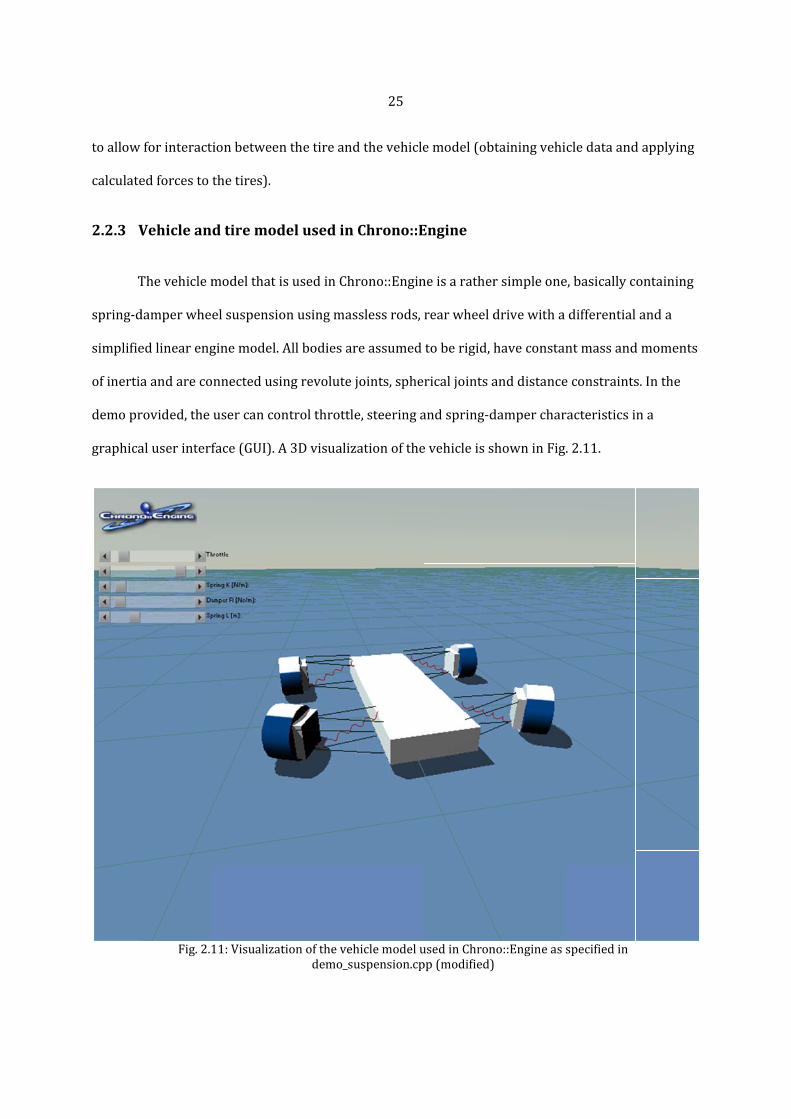
T
spring‐d
simplifie
ofinertia
demopr
graphica
forinteract
edforcesto
Vehiclean
Thevehiclem
damperwhe
edlineareng
aandareco
rovided,the
aluserinterf
Fig.2.1
tionbetween
thetires).
dtiremod
modelthati
elsuspensio
ginemodel.A
onnectedusi
usercancon
face(GUI).A
11:Visualizat
nthetireand
delusedin
susedinCh
onusingmas
Allbodiesar
ngrevolute
ntrolthrottl
A3Dvisualiz
tionofthevehdemo_s
25
dthevehicle
nChrono::E
hrono::Engin
sslessrods,
reassumed
joints,sphe
le,steeringa
zationofthe
hiclemodeluuspension.cp
emodel(ob
Engine
neisarather
rearwheeld
toberigid,h
ricaljointsa
andspring‐d
evehicleiss
usedinChronpp(modified)
tainingvehi
rsimpleone
drivewitha
haveconsta
anddistance
damperchar
howninFig
no::Engineas
icledataand
e,basicallyc
differential
ntmassand
econstraints
racteristicsi
g.2.11.
specifiedin
dapplying
ontaining
anda
dmoments
s.Inthe
na

26
Thegeometryofthevehicleaswellasthetransmissionandenginesetupandthesuspension
systemaredefinedinthe“MySimpleCar”class.Thismakesiteasiertomanagedataflowsuchas
calculationandapplicationofthewheeltorque.Thesimpletiremodelusedinthismodelisfriction‐
based,sotimeevolutionofthevehicleiscalculatedbysolvingthecontactproblembetweenrigid
bodies(tiresandground)atgivenfrictioncoefficientsandwheeltorque.
Thewheeltorqueiscomputedateverytimestepofthesimulationusinginformationsuchas
throttle(userinput),wheelspeed,finaldriveratioandgearratio.Thetorquecurveoftheengineis
assumedtobelineartokeepthemodelsimple.
2.2.4 TheStandardTyreInterface(STI)
In1997,theso‐calledStandardTyreInterface(STI)wasintroducedbytheinternational
TYDEXworkshopasastandardFORTRAN‐77interfacebetweenvehicle,tireandroadmodel[8].
Theuseofastandardizedinterfacemakesitpossibletoswitchbetweendifferenttiremodels
withouttheneedtomodifythevehicleorroadmodels[13].STIfeaturesanexchangeofallthe
necessaryinformationtoconnectroad,tireandvehiclemodel(cf.Fig.2.12)andalsodefines
coordinatesystemsandphysicalunits(SI).TheTYDEXworkshopalsodefinedtheTYDEXfileformat
tostandardizestorageoftiredataobtainedfromexperimentalmeasurements.

T
thetirem
1
2
3
4
5
6
7
F
between
approac
canbefo
Thefollowin
modelwhen
1) Current
2) Kinemat
3) Forcesan
4) Statevar
5) Signalsfo
6) Tirespec
7) Workarr
Furthermore
nroad,tirea
htheroadis
oundin[14]
nginformatio
nusingSTI[8
simulationt
ticinformati
ndtorquesa
riables,state
forpost‐proc
cificparame
raytostore
e,roadinfor
andvehiclem
sassumedto
].
Fig.2.12:S
onistransfe
8]:
time
ononmotio
appliedtoth
ederivatives
cessing
etersandnam
internalcom
rmation(like
modelusing
obeplanar.
27
Schematicvie
erredbetwe
onofthewh
hewheelcen
sandinitial
meofthetir
mputationre
ealtitude a
STI.Howev
Thefulldes
ewoftheSTI
enthemulti
eelcenter
nter
conditions
repropertyf
esultsofthe
anditsderiv
ver,inthissi
scriptionofv
[8]
ibodysystem
file
etiremodel
vatives)can
mplifiedimp
variablesan
m(MBS)solv
beexchange
plementatio
ndarraysuse
verand
ed
on
edinSTI

28
2.2.5 OrganizationoftheMagicFormulatiremodelinChrono::Engine
InsideChrono::Engine,theMagicFormulatiremodelisorganizedasaclass,“PacejkaTire”,
whichincludesallthenecessarysubroutines,structuresandvariablesthatareneededtodefinethe
tireproperties,theStandardTyreInterfaceandtheconnectiontothevehiclemodel,inthissimple
casethedemovehicle“MySimpleCar”.Twofilesdescribethemodel:“pacejka_definitions.h”,a
headerfilethatcontainsclassdefinitionandfileincludes,and“pacejka_functions.cpp”,which
incorporatestheactualsubroutinesusedbythe“PacejkaTire“class.Uponexecutingthemain
functionofthesimulation,fourtireobjectsarebeinginitialized,eachwithanindependentMagic
Formulamodel(whichalsoallowsfordifferent.tirepropertyfilesforeachtire)andauniquetireID.

29
2.2.6 Obtainingreal‐timevehicledata
Ahighlyaccuratetiremodelmakesitimperativetousereal‐timedatafromthevehicle
model.Forthispurpose,thegetVehicleData()subroutineusesvectorsandtransformation
matricesprovidedbytheChrono::Engineenvironmenttocalculatevehicleandtireinformationsuch
aswheelspeedofrevolution orsideslipangle ,whichistheanglebetweenthez‐axisofthe
wheelspindleanditsabsolutevelocity spindle wheel xV V V .Calculationofthesequantitiestakes
placeateveryintegrationstepofthedynamicssolverandisperformedseparatelyforeachtire.
Fig.2.13:Vectorsusedtodescribethemovementofthevehicle
Toavoidsingularitieswhichcouldhavenegativeimpactonthequalityofslipdataandforce
calculationsofthetiremodel,specialstepsaretakenforcriticalsituations,e.g.whenawheelisata
standstillandtherefore 0spindleV ,whichwouldresultinunrealistic,arbitraryslipangles and
potentiallydisturbthesimulation.
wheelV
chassisV
spindlezvehicle path
wheel path
wheel

30
Asanexampleofinteractionofvehiclemodelandtiremodel,acodesnippetofthe
getVehicleData()subroutineisshowninFig.2.14.Inthissectionofthecode,thewheelangular
velocity andspindlevelocityareusedtocalculatelongitudinalvelocity wheel xV V ofthewheel,
whichisanelementaryinputtotheMagicFormula.
Fig.2.14:CodesnippetofthegetVehicleData()subroutine
FollowingthesamestructureasintheMATLABimplementation,thevehicledatacanthen
beusedtodetermineforces ,,x y zF F F andmoments , ,x y zM M M usingcomputeForces()(called
transientMF.mintheMATLABcodeofFig.2.2)anditssubroutines.
switch (stiParameters.IDTYRE)case1:
// left front tire (tireID 1)
// wheel position in global RF ------------------------------------------------------------stiParameters .DIS[1] = mWheelLF ‐>get_ptr ()‐>GetPos().x;stiParameters .DIS[2] = mWheelLF ‐>get_ptr ()‐>GetPos().y;
stiParameters .DIS[3] = mWheelLF ‐>get_ptr ()‐>GetPos().z;
// wheel rotation in local RF --------------------------------------------------------------ChVector <>wheelRotationLRF = mWheelLF ‐>get_ptr ()‐>GetWvel _loc();stiParameters .OMEGAR = ‐wheelRotationLRF .y;
if (stiParameters.OMEGAR > 0)vehicleData.travelDirection = 1.0;
else
vehicleData.travelDirection = ‐ 1.0;
// -------------------------------------------------------------------------------------------------// transform spindle orientation to global reference frameChMatrix 33<>*spindleMatA = mSpindleLF ‐>get_ptr()‐>GetA ();ChVector <>spindleOrientation = spindleMatA ‐>Matr_x_Vect(VECT_Z);
ChVector <>spindleVelocity = mSpindleLF ‐>get_ptr()‐>GetPos _dt();
// calculate V _x -------------------------------------------------------------------------------vehicleData.V_x = vehicleData .travelDirection *sqrt(spindleVelocity .x *
spindleVelocity .x + spindleVelocity .z * spindleVelocity .z);

31
2.2.7 Applicationoftheforcesandmomentstothevehiclemodel
Inordertoapplythetireforcesandmomentstothevehicle,anewreferenceframeis
attachedtothecontactpatchofeachtire.Theprimarypurposeofthistirereferenceframeisto
transformtheforcesandmomentsobtainedthroughtheMagicFormulasubroutines(andexpressed
inthelocaltirereferenceframe)totheglobalreferenceframeusingthetransformationmatrix A .
Thustheforcesandmomentscaneasilybeappliedtothewheelobjectsinglobalcoordinatesusing
Chrono::Engine’sAccumulate_force() function.
TheverticalforceoftheChrono::Engineimplementationismodeledasaspringforce,
linearlydependingonthedeflectionofthetire.Therefore,thecollisioncontactbetweenwheelsand
groundhasbeendeactivatedtoallowthetires(rigidbodiesinthismodel)tosinkintotheground,
simulatingthetires’deflectionunderload.Inthisway,thevehicleisfloatinginanequilibriumof
normalload(staticanddynamic)andnormalforcesproducedbythetires.
TheverticalforceintheMagicFormulamodelcanbeobtainedusing
01
0
'zz z z Cz
FF p
R and (2.1)
0max(( )cos( ) (1 cos( )),0)z l cr r r , (2.2)
where lr istheloadedtireradius, 0r istheunloadedtireradiusand cr istheradiusofthe
approximatelycirculartirecontour[3].Theotherparametersarespecificfortherespectivetire.
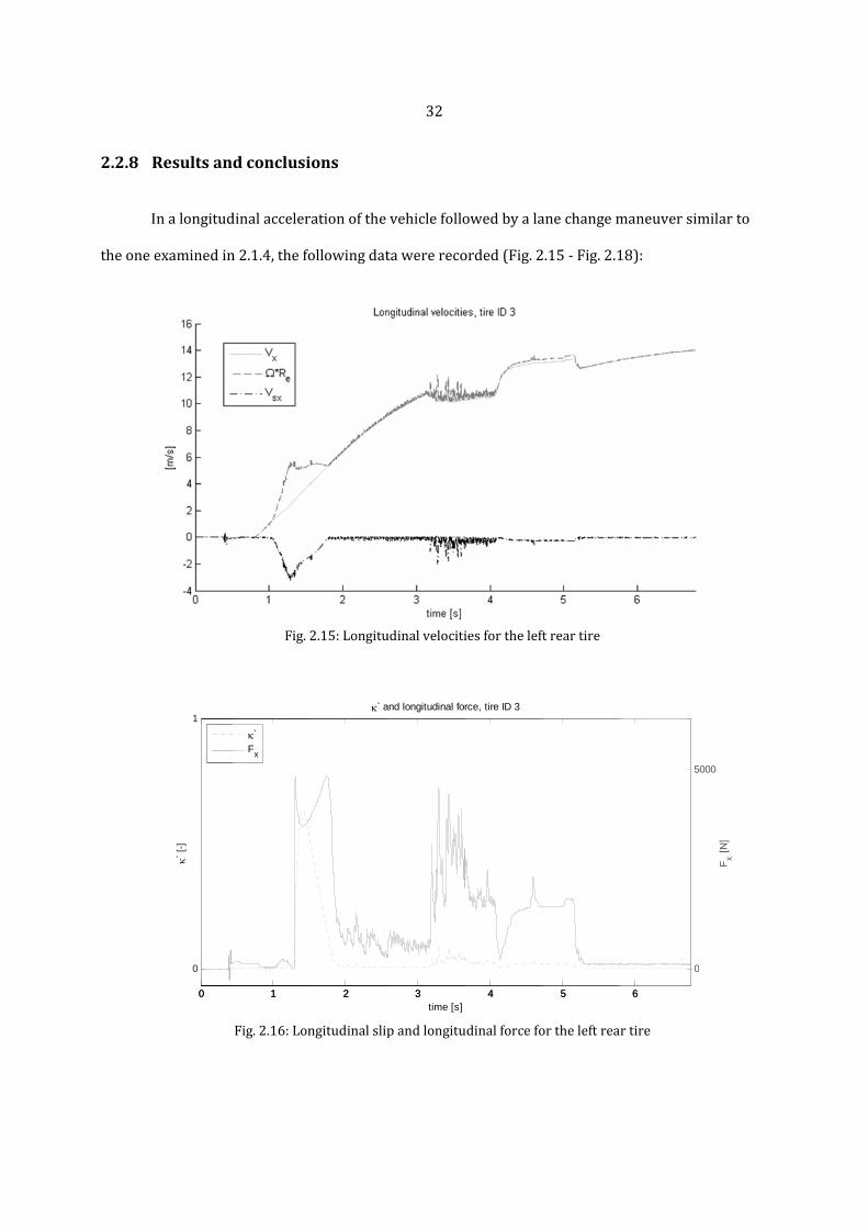
2.2.8 R
I
theonee
Resultsan
Inalongitud
examinedin
0
0
1
` [
-]
0
dconclusi
dinalacceler
n2.1.4,thefo
Fig.2
Fig.2.16:Lon
11
`
Fx
ions
rationofthe
ollowingdat
2.15:Longitu
ngitudinalslip
2
` a
2
32
vehiclefollo
tawerereco
udinalvelociti
pandlongitu
3time [s]
and longitudinal for
3
owedbyala
orded(Fig.2
iesfortheleft
udinalforcefo
4
rce, tire ID 3
4
anechangem
2.15‐Fig.2.1
ftreartire
ortheleftrea
55
maneuversi
18):
rtire
6
6
0
5
milarto
0
5000
Fx [
N]

33
Fig.2.17:Sideslipangleandlateralslipvelocityfortheleftfronttire
Fig.2.18:Transientslipangleandlateralforcefortheleftfronttire
0 1 2 3 4 5 6-4
-3
-2
-1
0
1
2
3
4
time [s]
[-]
[m/s
]Side slip and lateral slip velocity, tire ID 1
V
sy
0 1 2 3 4 5 6-0.5
0
0.5
time [s]
`
[-]
` and lateral force, tire ID 1
0 1 2 3 4 5 6-5000
0
5000
Fy [
N]
`
Fy

34
AsitcanbeseeninFig.2.15andFig.2.16,thelongitudinalaccelerationoftherear‐wheel
drivenvehiclecauseslongitudinalslip(duetothedifferencebetween xV and eR )andtherefore
alongitudinalforce, xF .Thepeaksin eR and sxV arecausedbywheelspinduringacceleration.
Theactuallanechangeisbestexaminedforthesteeredfronttires(Fig.2.17‐Fig.2.18).In
Fig.2.17,thesideslipangle andlateralslipvelocity syV areshownfortheleftfronttire.The
correspondingtransientslipangle ' andthelateralforce yF areshowninFig.2.18.
InFig.2.16andFig.2.18,itcanbeseenthatespeciallythecalculatedlongitudinalforceson
thedrivenwheels,butalsothelateralforcesaresubjecttoheavyoscillations.Thiscouldbefor
severalreasons,likenoiseandalackofdampingintheinputparameters.However,asmentionedin
1.2.2,thesimplecontactpointmodelusedtocalculatetransientslipquantitiesislimitedtolow
slippages.Toavoidsuchproblems,switchingtoamoreadvanced,butalsomorecomplexand
computationallymoreexpensivetransientmodeltoproduceinputdatafortheMagicFormula
modelmightbeconsidered.

35
3 Beamtiremodelforinteractionwithdeformableterrain
Thesemi‐empiricalPacejkaMagicFormulatiremodeldescribedinthepreviouschaptersis
veryaccurateonrigidterrainandpowerfulforreal‐timeapplications.Itis,however,alsorelianton
precedingprecisemeasurementsoftherespectivetire.FurtherpracticalissuesoftheMagic
Formulatiremodelindailyworkhavebeendescribedin[15].Also,itthemodelisnotcapableof
interactingwithdeformable,undulatedterrainsuchassoil,sandorsnow.Foroff‐roadvehicle
applicationsthisinteractionisanimportantfactorthathastobeconsideredandthetiremodel
shouldbeabletohandle.Allowingfordeformableterrainalsotakesintoaccounttherolling
resistanceduetoelastichysteresisofthegroundandbulldozingresistancewhengroundmaterialis
pushedinfrontofthecontactpatchofthetire[5].Thereforeinthischapteraphysics‐basedtire
modelusingabeam‐basedapproachissuggested.
3.1 Tiretreadmodel
Inthismodel,thetiretreadisrepresentedbyasetofmasslessthinbeamswithequivalent
springstiffnesses /axialk AE L (axial)and 3 3 /lateralk EI L (lateral)[16].Theradialbeamsare
connectedtothewheelrimatonesideandarelinkeduptoeachotherattheothersidewithshort
connectingbeamstoformanet,simulatingthetiretread(Fig.3.1).Thisconfiguration,also
consideringfrictionbetweenthebeamtippoints(furtherreferredtoas“elements”)andground,
allowsforlongitudinalaswellaslateralflexibilityandthereforeslipinxandydirectionstoinduce
longitudinalandlateralforcesinthecontactpatch.Itisimportanttonotethatthetireisnottreated
asadynamicsystemwithmassesandequationsofmotionassociatedwithit,butasaforceelement.
Thisisjustifiedbytheobservationthat,whenconnectedtoavehiclemodel,nottheforcesinsidethe
tireareofinterest,buttheforcesthatareappliedtothewheelhub.Consequently,itisassumedto

36
besufficienttoobtaintheequationsofmotionforthewheel,therebyconsideringtheforcescreated
bythedeflectionofthebeams.
rz
Fig.3.1:Beamelementsetupforthetiretread:anetofbeamsconnectedtotherim
Forsimplicityandtolimitcomputationalcostofthesimulation,bendingandtorsional
momentsinthebeamsarebeingneglectedandsmalldisplacementsandrotationsareassumed.

37
3.2 Forcesinthetiretreadandcontactpatch
Sincethecontactpatchismodeledasacollectionofbeamsorientedinlongitudinal,lateral
andradialdirection,numerousforcesbetweenthebeamshavetobeconsidered.Theseforcesarea
resultoftherelativedisplacementoftheelementswithrespecttoeachotheraswellasthewheel
rimduetoloadonthetireandinteractionwithground(friction,normalforce).Asideviewofthe
tirewithforcesin and r directionisshowninFig.3.2.
,i jr, 1i jr
, 2i jr
, 1i jr ,i jrF
,i jF
,i jF
Fig.3.2:Circumferentialandradialforcesatelement(i,j)
Theradialforces rF representthetirecarcassstiffnessandtheairpressureinsidethetire
andcausedeformationoftheterrainunderthecontactpatchifthegroundisnotrigid.Atopview
schematicoffiveelementsofthetiretreadandthecorrespondingforcesisshowninFig.3.3.

38
1F
2F
1zF 2zFrF
r z
1,i j
, 1i j
, 1i j
1,i j
,i j
Fig.3.3:Setofforcesactingononeelement(i,j)
Theforcesactingonanelement ,i j andresultingfromtherelativedeflectionofthebeams
toeachotheraswellastheradialdeflectionwithrespecttotheunloadedtireradiuscanbe
calculatedasfollows(cf.Fig.3.3):
I. Forcesin direction:
Force ,1F duetolongitudinaldeflectionofbeam1:
,1 , , , 1 ,( )axial i j i j i j refF k r (3.1)
Force ,2F duetolateraldeflectionofbeam2:
,2 , , 1, ,( )z lateral i j i j i jF k r (3.2)
39
Force ,3F duetolateraldeflectionofbeam3:
,3 , , 1, ,( )z lateral i j i j i jF k r (3.3)
Force ,4F duetolongitudinaldeflectionofbeam4:
,4 , , , , 1( )axial i j i j i j refF k r (3.4)
Force ,5F duetolateraldeflectionoftheradialbeam:
,,5 , , , 0 0( )i jr lateral i j i jF k r r
(3.5)
Thesumofforcesinthe directionforoneelement ,i j istherefore:
,
, , , , 1 , , , 1, ,
, , 1, , , , , , 1
, , , 0 0
( ) ( )
( ) ( )
( )i j
i axial i j i j i j ref z lateral i j i j i ji
z lateral i j i j i j axial i j i j i j ref
r lateral i j i j
F F k r k r
k r k r
k r r
(3.6)
II. Forcesin z direction:
Force ,1zF duetolateraldeflectionofbeam1:
,1 , , 1 ,( )z lateral i j i jF k z z (3.7)
Force ,2zF duetolongitudinaldeflectionofbeam2:
,2 , , 1,( )z z axial i j i j refF k z z z (3.8)
40
Force ,3zF duetolongitudinaldeflectionofbeam3:
,3 , 1, ,( )z z axial i j i j refF k z z z (3.9)
Force ,4zF duetolateraldeflectionofbeam4:
,4 , , 1 ,( )z lateral i j i jF k z z (3.10)
Force ,5zF duetolateraldeflectionoftheradialbeam:
,,5 , , 0( )i jz r lateral i jF k z z (3.11)
Thus,thesumofforcesinthe z directionforoneelement ,i j is:
,
, , , 1 , , , 1,
, 1, , , , 1 ,
, , 0
( ) ( )
( ) ( )
( )i j
z z i lateral i j i j z axial i j i j refi
z axial i j i j ref lateral i j i j
r lateral i j
F F k z z k z z z
k z z z k z z
k z z
(3.12)
III. Forcesin r direction:
Force ,1rF duetolateraldeflectionofbeam1:
,1 , , 1 ,( )r lateral i j i jF k r r (3.13)
Force ,2rF duetolateraldeflectionofbeam2:
,2 , 1, ,( )r z lateral i j i jF k r r (3.14)
Force ,3rF duetolateraldeflectionofbeam3:

41
,3 , 1, ,( )r z lateral i j i jF k r r (3.15)
Force ,4rF duetolateraldeflectionofbeam4:
,4 , , 1 ,( )r lateral i j i jF k r r (3.16)
Force ,5rF duetoradialdeflectionofthecenterelement(thisincorporatestireinflation
pressureandcarcassstiffness:
,5 , ,( )r r axial ref i jF k r r (3.17)
Theresultingradialforceis
, , , 1 , , 1, ,
, 1, , , , 1 ,
, ,
( ) ( )
( ) ( )
( )
r r i lateral i j i j z lateral i j i ji
z lateral i j i j lateral i j i j
r axial ref i j
F F k r r k r r
k r r k r r
k r r
. (3.18)
Bysumminguptheforcesofalltheelementsthatarepartofthecontactpatchin , r and
z direction,wecanthenobtaintheoverallforces(andmoments)actingontherim.
3.3 Modelverification
Thebeammodelisimplementedintoasimulationenvironmentandverifiedusingaself‐
writtenMATLAB2DsimulationenginecalledSimEngine2D,developedinProfessorDanNegrut’s
“ME451:Kinematics&DynamicsofMachineSystems”classattheUniversityofWisconsin‐Madison.
SimEngine2Dfeaturesstandardizeddatainput(twodatafilestocharacterizetheanalysisandthe
desiredmodel)andusesaNewmarkintegratortoperformdynamicsanalysis.Theadvantageofthis
simulationpackageisitsversatileandhighlycustomizablecode,facilitatingtheimplementationof
thetiremodelasasetofforceelementsaswellasitsattachmenttotherigidbodyrim.However,

42
sincethesoftwareislimitedto2‐dimensions,onlyverticalandlongitudinalmotionofthewheelcan
beexamined.
3.3.1 Verticalmotionofthewheel
Thenormalforceisverifiedby“dropping”thetire(with240elementsin4layers)tothe
groundfromaheightof0.35m(theunloadedtireradiusbeing0.305m).Sinceaflexibleterrain
modelhasn’tbeenimplementedyet,thegroundisassumedtobenon‐deformable.However,the
respectiveelementscouldinteractwiththeterrainaswell.
Wewouldexpectthetiretodeflectradiallyinthecontactpatchzoneandtherebydevelopa
resultingverticalforcethatcounteractsthegravitationalinertiaofthetire.Indeed,thetire
successivelydeformsasithitstheground(cf.Fig.3.4andFig.3.5)andaverticalforce(thesumof
theforcesatalloftheelements,Fig.3.6)pushesthewheelbackupsothatitstartsbouncingupand
downcontinuously(Fig.3.7).
Fig.3.4:Deflectedtireandresultingnormalforcesduetocontactwithground
(t=0.125s‐2Dview)
-0.5 -0.4 -0.3 -0.2 -0.1 0 0.1 0.2 0.3 0.4 0.5
-0.4
-0.3
-0.2
-0.1
0
0.1
0.2
0.3

43
InFig.3.6andFig.3.7,itcanbeobservedthatdampingoccurs(theamplitudedecreases)–
however,thisisduetonumericalintegrationdampingsincethebeamtiremodelitselfdoesn’t
includeatthistimeanymechanicaldamping.
Fig.3.5:Deflectedtireandresultingnormalforcesduetocontactwithground
(t=0.125s‐3Dviewofcontactpatch)
Fig.3.6:ResultingverticalForcedevelopedinthetirecontactpatch
0 0.2 0.4 0.6 0.8 1 1.2 1.4 1.6 1.8
0
200
400
600
800
1000
1200
1400
1600
1800
time [s]
Fr [
N]

3.3.2 L
F
contactp
direction
between
relatedt
I
Fig.3.7
Longitudin
Forlongitud
patchisnece
nandthusin
ntheelemen
totheonede
Inthecaseo
z
7:Verticalmo
nalmotion
dinal(andlat
essaryinord
nducelongit
ntsandgrou
escribedin[
ofbraking( v
1 0
0
.
ovementofth
nofthewh
teral)motio
dertodeflec
tudinalandl
ndinlongitu
[17]isused
v r ),the
44
hewheelhub
eel
nofthetire
cttheeleme
lateralforce
udinaldirec
(Fig.3.8):
normalized
center(integ
,frictionbet
ntsincircum
es,respectiv
ction,akinem
dlongitudina
grationsteps
tweentirea
mferential(
ely.Tomode
matic‐based
alslip z isde
ize:0.001s)
ndgroundin
)orlatera
elfrictional
frictionmo
efinedas
nthe
al( z )
contact
del
(3.19)

F
yields
forbraki
fordrivi
T
motionb
Forsimplicit
bs
ing( ,v r
ds
ng( ,v r
Toobtainth
betweenthe
,i j
F
ty,however,
1r
v
,
, 0v )and
1v
r ,
0 ).
edeflection
ebeamelem
,0 ,i j i js
Fig.3.8:Kinem
,insteadwe
s(cf.Fig.3.2
entsandgro
,
45
matic‐basedf
usethedefi
2and 1
ound,thefol
frictionmode
initionofsli
0 inFig.3.8)
llowingemp
el[17]
pasalready
resultingfr
piricalrelatio
ydefinedin(
romtherelat
onisused:
(1.2)‐this
(3.20)
(3.21)
tive
(3.22)

46
where ,i j istheactualangularcoordinate(polarcoordinatesystem)oftheelement ( , )i j ,,0i j
is
thereferenceangularcoordinateoftheundeformedelement(free‐rollingtire), s isslipforbraking
ordriving, isthekinematicfrictioncoefficientbetweentireandground,and isacorrection
factor.
Thus,theprocessofdevelopinglongitudinalforcesinthetirecontactpatchisthefollowing:
Withthewheelspinning(forexamplebyapplyingatorquetothewheelhub)orbypullingthetire,
relativemotionbetweenthetireandground(i.e.slip)results,causingthebeamelementsinthe
contactpatchtodeformin directionasdepictedinFig.3.8.Thisgivesrisetoalongitudinal
reactionforcethatcanbecalculatedusingtheequationsintroducedin3.2andthateventually
contributestothegeneralizedforcesappliedtothewheelinSimEngine2D.
Toverifythisprocess,thefollowingscenarioshavebeenimplementedinSimEngine2D:
A.Pullingthe(non‐rotating)wheeloverground,thewheelshouldstartturning;
B.Rotatingthewheelhub,alongitudinalmotionshouldresult.
Foreachscenario,thefollowingvaluesareused:
kinematicfriction(constant) 0.4
correctionfactor 0.25
unloadedtireradius 0.305refr m
loadedtireradius 0.295r m
radiusoftherim 0.2rimr m
tirewidth 0.2b m
Theequivalentspringstiffnessesareasfollows:
beamsin direction:
axial , 100axialNk m
lateral , 100lateralNk m
beamsin z direction:
axial , 100z axialNk m
lateral , 100z lateralNk m
beamsin r direction:
axial , 5000r axialNk m
lateral , 100r lateralNk m

I
speedof
thewhee
InscenarioA
f 0.5v m
eltostartro
Fig
A,thewheel
s .Through
otating(cf.F
g.3.9:Scenari
(1080elem
themechan
Fig.3.9):
oA:angularp
47
mentsin3lay
ismsdescrib
position,velo
yers)ispulle
bedabove,t
ocityandacce
edhorizonta
thetireelem
elerationofth
allyatacons
mentdeflectio
hewheel
stant
onscause

T
coincide
F
correspo
zero,the
I
standstil
therotat
(Fig.3.1
Theangular
eswiththea
Figure3.10s
ondingsum
elongitudina
InscenarioB
llandarota
tionistrans
1):
velocityapp
ngularveloc
showsthed
oflongitudi
alforcealso
B,thewheel
ation(
formedtoa
proachesan
cityofafree
ecreaseofb
nalforcesof
decreasesa
Fig.3.10:Sl
(withtirem
0.4 rad s
longitudina
48
asymptotic
e‐rollingwhe
brakeslipas
falltheelem
andeventua
ipandtotallo
modelspecifi
s )isapplied
almotionby
maximumo
eel:
thewheelst
mentsinthe
llybecomes
ongitudinalfo
icationssim
dtothewhee
thetireelem
of 1.695
0.5 0v r
tartsrotatin
contactpatc
zeroforthe
orce
milartoscena
elhub.Thes
mentsalmos
rad s ,whic
0.295 1.695
ngandthe
ch.Asslipap
efree‐rolling
arioA)isini
simulations
stinstantane
ch
5rad s .
pproaches
gwheel.
tiallyat
howsthat
eously

S
accelera
velocity
Similartosc
ationofthew
plots,tracti
Fig.3.11:Sce
enarioA,th
wheeldecrea
onisbuiltu
enarioB:xve
etotallongi
asesasslipd
pveryquick
49
elocityandac
tudinalforc
decreases(F
kly.
ccelerationof
e F andthe
Fig.3.12).As
fthewheelce
ereforethel
sitcanbese
enter
longitudinal
eeninthesli
ipand

50
Fig.3.12:ScenarioB:Slipandtotallongitudinalforce
3.4 Resultsandfuturework
Thebeamtiremodel’sfunctionalityhasbeenshownintheprecedingchapter.However,this
rathersimplemodelstillneedsvalidation–e.g.sincetheelementdeflectionsandthereforeforce
calculationsarelinear,thismodelmightberestrictedtosmallslipconditions,wherethefriction
coefficientandthelongitudinalforcearenearlylinearfunctionsofslip.
Anoff‐roadimplementationofthetiremodelfurthermorerequiresanappropriateinterface
betweentireandflexibleterraintoobtaintheradial,circumferentialandlateraldeflectionsofthe
beamelements.Foroff‐roaduse,factorssuchassinkagealsohavetobeconsidered,resultingin
higherrollingresistance.Thisofcoursedependsontheterrainmodelused.
Also,sincethesimulationpackageusedispurely2D,portingtheimplementationofthetire
modeltoa3DengineorcommercialsoftwaresuchasMSCADAMScanbeconsidered.
0 0.02 0.04 0.06 0.08 0.1 0.12 0.14 0.16 0.18 0.20
500
time [s]
Fal
pha [
N]
0 0.02 0.04 0.06 0.08 0.1 0.12 0.14 0.16 0.18 0.20
0.5
1
slip
[-]
Falpha
slip
51
4 Summary
Inthiswork,thefocushasbeenonimplementingtwoverydifferenttiremodelsforusein
multibodydynamicssimulations.Thesemi‐empiricalPacejkaMagicFormulatiremodelhasshown
tobeaveryaccurateapproachonflat,rigidterrainbuthassomedifficultieswhenitcomestohighly
dynamicdrivingsituations.Also,itisnotsuitableforoff‐roadapplicationsthatrequireinteraction
withflexibleterrainorundulatedsurfaceswithshortwavelengths.
Forthisreason,asecondmodelhasbeenintroducedthatusesbeamstosimulatethetire.
Thisdiscretemodelhasaphysicalbackgroundbutisalsosubjecttolimitationsthatcouldbesolved
byextendingandfine‐tuningthemodel.Thismodelcertainlyisn’tsuitableforhighlydynamicon‐
roadapplicationsbuthasbeendesignedtosimulatee.g.construction‐typevehiclesmovingover
flexibleterrainsuchassoil,gravelorsand.

52
5 References
[1]EgbertBakker,LarsNyborg,andHansB.Pacejka,"TyreModellingforUseinVehicleDynamicsStudies,"SAEPaperNo.8704211987.
[2]EgbertBakker,HansB.Pacejka,andLarsLidner,"ANewTireModelwithanApplicationinVehicleDynamicsStudies,"SAEPaperNo.8900871989.
[3]HansB.Pacejka,TireandVehicleDynamics.Warrendale:SAEInternational,2006.
[4]AlessandroTasora.(2011)DeltaKnowledgeWebsite.[Online].http://www.deltaknowledge.com/chronoengine/
[5]GiancarloGentaandLorenzoMorello,TheAutomotiveChassis,Volume1:ComponentsDesign.Berlin:Springer,2009.
[6]Hans‐HermannBraessandUlrichSeiffert,HandbookofAutomotiveEngineering.Warrendale:SAEInternational,2005.
[7]AkiraHiguchi,"TransientResponseofTyresatLargeWheelSlipandCamber,"TU‐Delft,Dissertation1997.
[8]IgoJ.M.Besselink,"ExperienceswiththeTYDEXstandardtyreinterfaceandfileformat,"inTyreModelsforVehicleDynamicsAnalysis.London:Taylor&Francis,2005,vol.43Supplement1,pp.63‐75.
[9]DieterSchramm,ManfredHiller,andRobertoBardini,ModellbildungundSimulationderDynamikvonKraftfahrzeugen.Berlin:Springer,2010.
[10]FrancescoBraghinandEdoardoSabbioni,"ADynamicTireModelforABSManeuverSimulations,"TireScienceandTechnology,no.Vol.38,No.2,pp.137‐154,2010.
[11]JochenWiedemann,SkriptKraftfahrzeugeI(Wintersemester2009/2010).Stuttgart:InstitutfürVerbrennungsmotorenundKraftfahrwesen,UniversitätStuttgart,2009.
[12]AlessandroTasora,MarcoSilvestri,andPaoloRighettini,"ArchitectureoftheChrono:EnginePhysicsSimulationMiddleware,"inProceedingsofMultibodyDynamics.ECCOMASThematicConference,Milano,Italy,2007.
[13]J.J.M.VanOosten,H.‐J.Unrau,A.Riedel,andE.Bakker,"TYDEXWorkshop:StandardisationofDataExchangeinTyreTestingandTyreModelling,"VehicleSystemDynamics,no.27S1,pp.272‐288,1997.
[14]AndreasRiedelandUweWurster,"STI‐StandardizedInterfaceTyreModel‐VehicleModel(Release1.4),"Karlsruhe,1996.

53
[15]JochenRauhandMonikaMössner‐Beigel,"Tyresimulationchallenges,"VehicleSystemDynamics,no.46S1,pp.49‐62,2008.
[16]HorstIrretier,GrundlagenderSchwingungstechnikI.Braunschweig:Vieweg,2000.
[17]CarlosCanudas‐de‐Wit,PanagiotisTsiotras,EfstathiosVelenis,MichelBasset,andGerardGissinger,"DynamicFrictionModelsforRoad/TireLongitudinalInteraction,"VehicleSystemDynamics,no.39Issue3,pp.189‐226,2003.

54
A Appendix
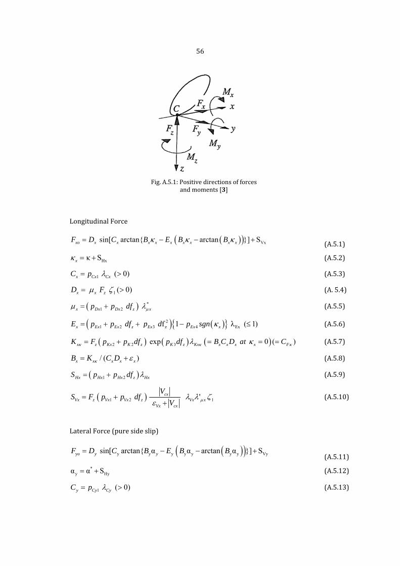
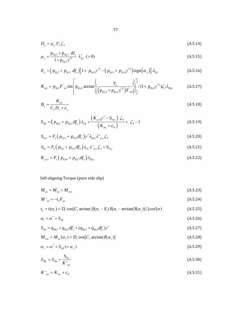
A.1 MagicFormulaequationsandfactors[3]
Parametersused
g accelerationduetogravity
cV magnitudeofthevelocityofthewheelcontactcenterC
,cx yV componentsofthevelocityofthewheelcontactcenterC
,sx yV componentsofslipvelocity sV (ofpointS)with s cyV V
rV ( )e cx sxR V V forwardspeedofrolling
oV referencevelocity(= ogR orotherspecifiedvalue)
oR unloadedtireradius ( )or
eR effectiverollingradius ( )er
wheelspeedofrevolution
z tireradialdeflection( 0 ifcompression)
zoF nominal(rated)load( 0 )
'zoF adaptednominalload: 'zo Fzo zoF F
Otherquantities
'
'z zo
zzo
F Fdf
F
normalizedchangeinverticalload
* tan( )sgn( )| |
cycx
cx
VV
V tangentoftheslipangle(forverylargeslipangles)
* sin spinduetocamberangle
| |sx
cx
V
V longitudinalslipratio
cos'( )'
cx cx
c c V
V V
V V
avoidsingularitiesat 0cV byaddingasmall 0.1V
1 ( 0,..,8)i i factors i canbesetequaltounitywhenturnslipmay
beneglected(pathradiusR )andcamber remainssmall

55
Userscalingfactors (defaultvalueofthesefactorsissetequaltooneifnotused)pureslip
Fzo nominal(rated)load
,x y peakfrictioncoefficient(lessthanoneforlowfrictionroadsurface)
V withslipspeed sV decayingfriction(defaultvalueisequaltozero!)
Kx brakeslipstiffness
Ky corneringstiffness
,Cx y shapefactor
,Ex y curvaturefactor
,Hx y horizontalshift
,Vx y verticalshift
Ky camberforcestiffness
Kz cambertorquestiffness
t pneumatictrail(effectingself‐aligningtorquestiffness)
Mr residualtorque
,*,
1
x yx y
sV
o
V
V
,
*,
, *,
'1 ( 1)
x yx y
x y
A
A
(suggestion: 10A )
combinedslip
x influenceon ( )xF
y influenceon ( )yF
Vy induced‘ply‐steer’ yF
s zM momentarmof xF
other
Cz radialtirestiffness
', ', ', '
,u v
overturningcouplestiffness
My rollingresistancemoment
L
F
C
D
E
K
B
S
S
L
F
α
C
Longitudinal
sinxo xF D
Hxκ Sx
1 x Cx CC p
x x zD F
1x Dxp
1x ExE p
x z KK F p
/ (x xB K C
1Hx HxS p
Vx z VS F p
LateralForce
yo sinyF D
*y Hα α S
1 y Cy CC p
lForce
n[ arctanxC
( 0)Cx
1 ( 0)
2 Dx zp df
2 Ex zp df p
2 2Kx K zp df
)x x xC D
2 Hx zp df
1 2 Vx Vx zp df
e(pureside
yn[ arctanC
Hy
( 0)Cy
Fig.A.5.1:
x x xB E B
*x
23 z f 1Exp d
3 exp Kp d
Hx
cx
Vx cx
V
V
eslip)
y y α yB E
56
Positivedireandmoment
arctax xB
4 Exp sgn
z Kxdf B
1 ' Vx x
y yα arctaB
ectionsofforcts[3]
an ]x xB
Ex λ (x
x x xB C D at
y yan α ]B
ces
VxS
1)
0 (x C
Vy] S
)FC
(A.5.1)
(A.5.2)
(A.5.3)
(A.5.4)
(A.5.5)
(A.5.6)
(A.5.7)
(A.5.8)
(A.5.9)
(A.5.10)
(A.5.11)
(A.5.12)
(A.5.13)
57
2 y y zD F (A.5.14)
Dy1 Dy2 z *μy*2
Dy3
p p df λ ( 0)
1 p γy
(A.5.15)
*2 *21 2 5 3 4 1 signy Ey Ey z Ey Ey Ey y EyE p p df p p p (A.5.16)
' *2z
1 Ky4 3 3*2 'Ky2 Ky5 z0
Fsin p arctan / (1 )
p p γ Fy Ky zo Ky KyK p F p
(A.5.17)
yy y y
yKB
C D
(A.5.18)
*0 0
1 2 4
1
y Vy
Hy Hy Hy z Hy
y K
K SS p p df
K
(A.5.19)
*3 4 2 ' Vy z Vy Vy z Ky yS F p p df (A.5.20)
1 2 2 ' Vy z Vy Vy z Vy y VyS F p p df S (A.5.21)
6 7y o z Ky Ky z KyK F p p df (A.5.22)
Self‐aligningTorque(puresideslip)
'zo zo zroM M M (A.5.23)
'zo o yoM t F (A.5.24)
( ) cos[ arctan ( arctan( ))]cos'( )o t t t t t t t t t tt t D C B E B B (A.5.25)
*t HtS (A.5.26)
*1 2 3 4( )Ht Hz Hz z Hz Hz zS q q df q q df (A.5.27)
( ) cos[ arctan( )]zro zr r r r r rM M D C B (A.5.28)
* ( )r Hf fS (A.5.29)
'Vy
Hf Hyy
SS S
K
(A.5.30)
'y y KK K (A.5.31)

58
2 * *21 2 3 5 6 *
( )(1 | | ) ( 0)Kyt Bz Bz z Bz z Bz Bz
y
B q q df q df q q
(A.5.32)
1( 0)t CzC q (A.5.33)
1 2( ) sgn'o
to z Dz Dz z t cxzo
RD F q q df V
F (A.5.34)
* *23 4 5(1 | | )t to Dz DzD D q q (A.5.35)
2 *1 2 3 4 5
2( )1 ( ) arctan( )( 1)t Ez Ez z Ez z Ez Ez t t tE q q df q df q q B C
(A.5.36)
9 10 6 9*( ) ( : 0)Ky
r Bz Bz y y Bzy
B q q B C preferred q
(A.5.37)
7rC (A.5.38)
*6 7 2 8 9 0
* * *10 11 0 8
( ) ( ) ...
... ( ) | | cos'( ) sgn 1
r z o Dz Dz z Mr Dz Dz z Kz
Dz Dz z y cx
D F R q q df q q df
q q df V
(A.5.39)
, 0 ( ~ , 0)( )zoz o to y y M
y
MK D K C
(A.5.40)
8 9( ) ( ~ , 0)( )zoz o z o Dz Dz z Kz to y o y M
MK F R q q df D K C
(A.5.41)
LongitudinalForce(combinedslip)
x x xoF G F (A.5.42)
cos[ arctan ( arctan( )) /x x x s x x s x s x oG C B E B B G (A.5.43)
cos[ arctan ( arctan( ))]x o x x Hxa x x Hxa x HxaG C B S E B S B S (A.5.44)
*s HxS (A.5.45)
*21 3 2( ) cos[arctan( )] ( 0)x Bx Bx Bx xB r r r (A.5.46)
1x CxC r (A.5.47)
1 2x Ex Ex zE r r df (A.5.48)
1Hx HxS r (A.5.49)

59
LateralForce(combinedslip)
y y yo VyF G F S (A.5.50)
cos[ arctan ( arctan( ))] /y y y s y y s y s y oG C B E B B G (A.5.51)
cos[ arctan ( arctan( ))]y o y y Hy y y Hy y HyG C B S E B S B S (A.5.52)
s HyS (A.5.53)
*2 *1 4 2 3( ) cos[arctan ( )]y By By By By yB r r r r (A.5.54)
1y CyC r (A.5.55)
1 2 ( 1)y Ey Ey zE r r df (A.5.56)
1 2Hy Hy Hy zS r r df (A.5.57)
5 6sin[ arctan( )]Vy Vy Vy Vy VyS D r r (A.5.58)
* *1 2 3 4 2( ) cos[arctan( )]Vy y z Vy Vy z Vy VyD F r r df r r (A.5.59)
NormalLoad
01
0
'zz z z Cz
FF p
R (A.5.60)
0max(( ) cos( ) (1 cos( )),0)z l cr r r (A.5.61)
( lr :loadedtireradius, cr :radiusofcirculartirecontour(approx.))
OverturningCouple
*1 2 3( )
'y
x z o sx sx sx Mxzo
FM F R q q q
F (A.5.62)
RollingResistanceMoment
1 2 arctan 'xr
y z o sy sy Myo zo
FVM F R q q
V F (A.5.63)
Self‐aligningTorque(combinedslip)
'z z zr xM M M sF (A.5.64)

60
' 'z yM tF (A.5.65)
, , , ,( ) cos[ arctan ( arctan( ))]cos'( )t eq t t t t eq t t t eq t t eqt t D C B E B B (A.5.66)
'y y VyF F S (A.5.67)
, ,( ) cos[ arctan( )]zr zr r eq r r r r eqM M D C B (A.5.68)
*1 2 3 4 ( )
'y
o sz sz sz sz z szo
Fs R s s s s df
F (A.5.69)
2 2 2, ( ) sgn( )
'x
t eq t ty
K
K
(A.5.70)
2 2 2, ( ) sgn( )
'x
r eq r ry
K
K
(A.5.71)
ExtensionofthemodelforTurnSlip(if t islarge,otherwise 1, 1,...,8i i )
2 0 4 0cos[arctan ( | | | |)]y t Dy tB R p R (A.5.72)
1 2 3(1 ) cos[arctan( tan )]y Dy Dy z DyB p p df p (A.5.73)
2 23 1 0cos[arctan( )]Ky tp R (A.5.74)
0 0 0sin[ arctan ( arctan( ))]Hy Hy Hy Hy Hy Hy HyS D C B R E B R B R (A.5.75)
1 2( )'
VyHy Hy Hy z Hy Hy
y
SS p p df S
K
(A..5.76)
*3 4 2( ) 'Vy z Vy Vy z Ky yS F p p df (A.5.77)
0 0 (A.5.78)
4 1'
VyHy
y
SS
K
(A.5.79)
1Hy HyC p (A.5.80)
2 3( ) sgn( )Hy Hy Hy z cxD p p df V (A.5.81)
4Hy HyE p (A.5.82)
0
0( )yR
HyHy Hy y K
KB
C D K
(A.5.83)

61
00 1
yyR
y
KK
(A.5.84)
1 2(1 )zp p df (A.5.85)
5 1 0cos[arctan( )]Dt tq R (A.5.86)
8 1 rD (A.5.87)
sin[ arctan ( arctan( ))]r Dr Dr Dr o Dr Dr o Dr oD D C B R E B R B R (A.5.88)
sin(0.5 )z
DrDr
MD
C
(A.5.89)
1 00'
zz Cr y z M
z
FM q R F
F (A.5.90)
1Dr DrC q (A.5.91)
2Dr DrE q (A.5.92)
0
( )(1 )z r
DrDr Dr r
KB
C D
(A.5.93)
0 0 8 9( )z r z Dz Dz z KzK F R q q df (A.5.94)
0 0 0 0z z r t yK K D K (A.5.95)
00 1
zzR
KK
(A.5.96)
6 1 0cos[arctan( )]Brq R (A.5.97)
90 2 0
2arctan( | |) ( )z z Cr t yM M q R G
(A.5.98)
907
2arccos[ ]
| |z
r r
M
D
(A.5.99)
1 0cos[arctan( )]xB R (A.5.100)
1 2 3(1 ) cos[arctan( )]x Dx Dx z DxB p p df p (A.5.101)

62
A.2 .tirepropertyfileusedintheMagicFormulaimplementations
%========================================================================== % Magic Formula parameters % Tire: 205/60R15 91V, 2.2bar (Pacejka, 2006) % Comments: %========================================================================== %-------------------------------------------------------------------------- % general parameters %-------------------------------------------------------------------------- % free unloaded tire radius R_0 = 0.313 % effective rolling radius (R_e = V_x / Omega_0) R_e = 0.305 % radius of the circular tire contour R_c = 0.15 % nominal (rated) load F_z0 = 4000 % reference velocity V_0 = 16.67 % tire stiffnesses C_Fx = 435000 % (taken from ADAMS file) C_Fy = 166500 % (taken from ADAMS file) %========================================================================== %-------------------------------------------------------------------------- % user scaling factors / default values %-------------------------------------------------------------------------- % pure slip lambda_Fz0 = 1.0 % 1.0 nominal (rated) load lambda_mux = 1.0 % 1.0 peak friction coefficient (x) lambda_muy = 1.0 % 1.0 peak friction coefficient (y) lambda_muV = 0.0 % 0.0 with slip speed decaying friction lambda_KxKap = 1.0 % 1.0 brake slip stiffness lambda_KyAlp = 1.0 % 1.0 cornering stiffness lambda_Cx = 1.0 % 1.0 shape factor (x) lambda_Cy = 1.0 % 1.0 shape factor (y) lambda_Ex = 1.0 % 1.0 curvature factor (x) lambda_Ey = 1.0 % 1.0 curvature factor (y) lambda_Hx = 0.0 % 1.0 horizontal shift (x) lambda_Hy = 0.0 % 1.0 horizontal shift (y) lambda_Vx = 0.0 % 1.0 vertical shift (x) lambda_Vy = 0.0 % 1.0 vertical shift (y) lambda_KyGam = 1.0 % 1.0 camber force stiffness lambda_KzGam = 1.0 % 1.0 camber torque stiffness lambda_t = 1.0 % 1.0 pneumatic trail lambda_Mr = 1.0 % 1.0 residual torque
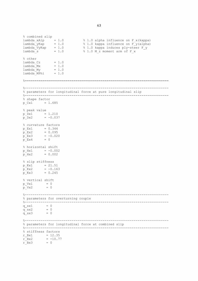
63
% combined slip lambda_xAlp = 1.0 % 1.0 alpha influence on F_x(kappa) lambda_yKap = 1.0 % 1.0 kappa influence on F_y(alpha) lambda_VyKap = 1.0 % 1.0 kappa induces ply-steer F_y lambda_s = 1.0 % 1.0 M_z moment arm of F_x % other lambda_Cz = 1.0 lambda_Mx = 1.0 lambda_My = 1.0 lambda_MPhi = 1.0 %========================================================================== %-------------------------------------------------------------------------- % parameters for longitudinal force at pure longitudinal slip %-------------------------------------------------------------------------- % shape factor p_Cx1 = 1.685 % peak value p_Dx1 = 1.210 p_Dx2 = -0.037 % curvature factors p_Ex1 = 0.344 p_Ex2 = 0.095 p_Ex3 = -0.020 p_Ex4 = 0 % horizontal shift p_Hx1 = -0.002 p_Hx2 = 0.002 % slip stiffness p_Kx1 = 21.51 p_Kx2 = -0.163 p_Kx3 = 0.245 % vertical shift p_Vx1 = 0 p_Vx2 = 0 %-------------------------------------------------------------------------- % parameters for overturning couple %-------------------------------------------------------------------------- q_sx1 = 0 q_sx2 = 0 q_sx3 = 0 %-------------------------------------------------------------------------- % parameters for longitudinal force at combined slip %-------------------------------------------------------------------------- % stiffness factors r_Bx1 = 12.35 r_Bx2 = -10.77 r_Bx3 = 0

64
% shape factor r_Cx1 = 1.092 % curvature factors r_Ex1 = 1.644; r_Ex2 = -0.0064359; % horizontal shift r_Hx1 = 0.007 %-------------------------------------------------------------------------- % parameters for lateral force at pure side slip %-------------------------------------------------------------------------- % shape factor p_Cy1 = 1.193 % peak values p_Dy1 = -0.990 p_Dy2 = 0.145 p_Dy3 = -11.23 % curvature factors p_Ey1 = -1.003 p_Ey2 = -0.537 p_Ey3 = -0.083 p_Ey4 = -4.787 p_Ey5 = 0 % slip stiffness p_Ky1 = -14.95 p_Ky2 = 2.130 p_Ky3 = -0.028 p_Ky4 = 2 p_Ky5 = 0 p_Ky6 = -0.92 p_Ky7 = -0.24 % horizontal shift p_Hy1 = 0.009 p_Hy2 = -0.001 p_Hy3 = 0 % vertical shift p_Vy1 = 0.045 p_Vy2 = -0.024 p_Vy3 = -0.532 p_Vy4 = 0.039 %-------------------------------------------------------------------------- % parameters for lateral force at combined slip %-------------------------------------------------------------------------- % stiffness factors r_By1 = 6.461 r_By2 = 4.196 r_By3 = -0.015 r_By4 = 0

65
% shape factor r_Cy1 = 1.081 % curvature factors r_Ey1 = 0 % (taken from ADAMS file) r_Ey2 = 0 % (taken from ADAMS file) % horizontal shift r_Hy1 = 0.009 r_Hy2 = 0 % (taken from ADAMS file) % vertical shift r_Vy1 = 0.053 r_Vy2 = -0.073 r_Vy3 = 0.517 r_Vy4 = 35.44 r_Vy5 = 1.9 r_Vy6 = -10.71 %-------------------------------------------------------------------------- % parameters for self-aligning moment at pure side slip %-------------------------------------------------------------------------- % stiffness factors q_Bz1 = 8.964 q_Bz2 = -1.106 q_Bz3 = -0.842 q_Bz5 = -0.227 q_Bz6 = 0 q_Bz9 = 18.47 q_Bz10 = 0 % shape factor q_Cz1 = 1.180 % peak values q_Dz1 = 0.100 q_Dz2 = -0.001 q_Dz3 = 0.007 q_Dz4 = 13.05 q_Dz6 = -0.008 q_Dz7 = 0.000 q_Dz8 = -0.296 q_Dz9 = -0.009 q_Dz10 = 0 q_Dz11 = 0 % curvature factors q_Ez1 = -1.609 q_Ez2 = -0.359 q_Ez3 = 0 q_Ez4 = 0.174 q_Ez5 = -0.896 % horizontal shift q_Hz1 = 0.007 q_Hz2 = -0.002 q_Hz3 = 0.147 q_Hz4 = 0.004

66
%-------------------------------------------------------------------------- % parameters for self-aligning moment at combined slip %-------------------------------------------------------------------------- s_sz1 = 0.043 s_sz2 = 0.001 s_sz3 = 0.731 s_sz4 = -0.238 %-------------------------------------------------------------------------- % parameters for normal load %-------------------------------------------------------------------------- p_z1 = 15.0 %-------------------------------------------------------------------------- % parameters for turn slip %-------------------------------------------------------------------------- p_DxPhi1 = 0.4 % (taken from ADAMS file) p_DxPhi2 = 0 % (taken from ADAMS file) p_DxPhi3 = 0 % (taken from ADAMS file) p_DyPhi1 = 0.4 % (taken from ADAMS file) p_DyPhi2 = 0 % (taken from ADAMS file) p_DyPhi3 = 0 % (taken from ADAMS file) p_DyPhi4 = 0 % (taken from ADAMS file) p_epsGamPhi1 = 0.7 % (taken from ADAMS file) p_epsGamPhi2 = 0 % (taken from ADAMS file) p_HyPhi1 = 1.0 % (taken from ADAMS file) p_HyPhi2 = 0.15 % (taken from ADAMS file) p_HyPhi3 = 0 % (taken from ADAMS file) p_HyPhi4 = -4.0 % (taken from ADAMS file) p_KyPhi1 = 1 % (taken from ADAMS file) % q_BrPhi1 = 0.1 % (taken from ADAMS file) q_CrPhi1 = 0.2 % (taken from ADAMS file) q_CrPhi2 = 0.1 % (taken from ADAMS file) q_DrPhi1 = 1.0 % (taken from ADAMS file) q_DrPhi2 = -1.5 % (taken from ADAMS file) q_DtPhi1 = 10.0 % (taken from ADAMS file) %-------------------------------------------------------------------------- % parameters for rolling resistance moment %-------------------------------------------------------------------------- q_sy1 = 0.01 % (taken from ADAMS file) q_sy2 = 0 % (taken from ADAMS file) %==========================================================================
Recommended