Graduate Theses, Dissertations, and Problem Reports
2021
Unconventional Gas Pipeline Right-of-Way Influence on Wildlife Unconventional Gas Pipeline Right-of-Way Influence on Wildlife
Samuel C. Knopka West Virginia University, [email protected]
Follow this and additional works at: https://researchrepository.wvu.edu/etd
Part of the Terrestrial and Aquatic Ecology Commons
Recommended Citation Recommended Citation Knopka, Samuel C., "Unconventional Gas Pipeline Right-of-Way Influence on Wildlife" (2021). Graduate Theses, Dissertations, and Problem Reports. 8000. https://researchrepository.wvu.edu/etd/8000
This Thesis is protected by copyright and/or related rights. It has been brought to you by the The Research Repository @ WVU with permission from the rights-holder(s). You are free to use this Thesis in any way that is permitted by the copyright and related rights legislation that applies to your use. For other uses you must obtain permission from the rights-holder(s) directly, unless additional rights are indicated by a Creative Commons license in the record and/ or on the work itself. This Thesis has been accepted for inclusion in WVU Graduate Theses, Dissertations, and Problem Reports collection by an authorized administrator of The Research Repository @ WVU. For more information, please contact [email protected].

Graduate Theses, Dissertations, and Problem Reports
2021
Unconventional Gas Pipeline Right-of-Way Influence on Wildlife Unconventional Gas Pipeline Right-of-Way Influence on Wildlife
Samuel C. Knopka
Follow this and additional works at: https://researchrepository.wvu.edu/etd
Part of the Terrestrial and Aquatic Ecology Commons

Unconventional Gas Pipeline Right-of-Way Influence on Wildlife
Samuel C. Knopka
Thesis submitted to the
Davis College of Agriculture, Natural Resources and Design
At West Virginia University
In partial fulfillment of the requirements
For the degree of
Master of Science
In
Wildlife and Fisheries Resources
John W. Edwards, Ph.D., Co-Chair
Shawn T. Grushecky, Ph.D., Co-Chair
Sheldon F. Owen, Ph.D.
Division of Forestry and Natural Resources
Morgantown, West Virginia
2021
Keywords: Fracking, natural gas, Pennsylvania, pipeline, pollinator, reclamation, ruffed grouse
salamander, snake, unconventional
Copyright 2021 Samuel C. Knopka

Abstract
Unconventional Gas Pipeline Right-of-Way Influence on Wildlife
Samuel C. Knopka
The development of horizontal drilling for natural gas in the Marcellus Shale in 2004
resulted in rapid exploitation of the play in the Appalachian Basin. This “unconventional” gas
well drilling accesses resources deeper beneath the surface and allows for multiple wells to be
co-located on a single well pad. This results in fewer, but larger, well pads on the landscape than
traditional vertical wells. Pipelines are required to transport the volumes of gas produced by
unconventional wells to production facilities and market. The effects of gathering pipelines,
which transport gas from well pads to larger transport pipelines, are poorly studied compared to
other types of disturbance.
This study evaluated how ruffed grouse (Bonasa umbellus), salamanders and snakes, and
pollinators use pipeline right-of-ways (ROW) in a forested environment. Forested areas of
Appalachia have undergone forest maturation and young forest habitat has declined. This habitat
modification led to declines of ruffed grouse and pollinator species. Although ROWs increase
forest fragmentation in large forest patches, they must be maintained as herbaceous vegetation to
protect pipeline integrity. The goals of this research were to determine how variation in ROW
reclamation influences wildlife use of these ROWs. Difference in use can provide
recommendations that enable ROWs to provide the most benefit to these species, and if they
could act as an analogue for early successional habitat.
All research was conducted on the Tiadaghton State Forest and Game Commission Game
Lands 12, two land parcels in North-Central Pennsylvania managed by the state. These areas are
heavily forested and contain a network of natural gas ROW that varied in age, width, and
reclamation. Surveys from ruffed grouse and pollinators were conducted on these sites from May
–August 2019 and 2020. Cover boards used to sample for reptiles and amphibians were deployed
in summer 2019 and surveyed from May — August 2020.
Too few ruffed grouse were observed during surveys to perform analysis, but incidental
observations of white-tailed deer (Odocoileus virginianus) and eastern wild turkeys (Meleagris
gallopavo) on ROWs suggests that they provide some benefits to these species. Eastern red
backed salamanders (Plethodon cinereus) were used as a case study to examine the effects of the
ROW on forest salamanders. Salamander occupancy increased as distance from the ROW edge
increased, due to the negative effects of edge. Occupancy overall decreased as ROW age
increased, and occupancy at all distances from the ROW edge decreased as ROW age increased.
This suggests that edge effects degrade habitat along ROW over time, and that edge effects
influence adjacent forest for at least 30m (farthest cover boards from the ROW edge). Snakes
were observed on the ROW more than on the edge or in forest, and rodents were observed at
most ROW sites. These suggest that snakes are more likely to utilize ROWs and that prey
abundance is higher. Pollinators were more likely to be found at sites with higher percentages of
flowering forbs. Butterfly species richness, butterfly density, and bee density were all positively
related to the percent of flowers on the ROW. Pollinator density of each transect (10m ×100m)
was not related to total ROW width, indicating that pollinator density is a function of flower

abundance rather than an interaction between width and flower abundance. This suggests that
pollinator abundance would increase as ROW width increases assuming flower percentage
remains constant.
For the species in this study, ROW width negatively impacts forest salamanders but can
be beneficial to snakes and pollinators. Differences in seed mix will change available food
resources and vegetative structure. The best reclamation plan will vary based upon the
circumstances and most imperiled species at each location. Overall, ROWs should be located
along existing disturbance in forested areas to limit additional forest fragmentation. Reclamation
should include seed mixes that prioritize native plants and maximize flowering throughout the
growing season. The temporary workspace of each ROW should be replanted with fruiting trees
and shrubs to increase forage for wildlife and soften the forest edge to reduce edge effects on
salamanders. A ROW with these characteristics provides a balance between wildlife while
providing resources which would otherwise be absent.

iv
Acknowledgments
I would like to sincerely thank both of my co-advisers Dr. John W Edwards and Dr.
Shawn T Grushecky for their assistance with all aspects of my master’s degree, from class choice
to research. I am grateful for this opportunity at West Virginia University, and feel that the
interdisciplinary background of my co-advisers improved my learning experience. I would also
like to thank the third member of my committee, Dr. Sheldon Owen, for his assistance and
expertise with the pollinator portion of my research and thesis. This research would not have
been possible without the help of the Pennsylvania Game Commission and Department of
Conservation and Natural Resources. Dr. Linda Ordiway (formerly of the Ruffed Grouse
Society, currently with the WV Department of Natural Resources) was also instrumental in
providing assistance to the planning phase of the ruffed grouse portion of this project. Kevin, a
fellow graduate student, helped tremendously with forestry measurements of my study sites as
well. Finally, I would like to thank my family and loved ones for their support during my time at
WVU.

v
Table of Contents
Abstract ........................................................................................................................................... ii
Acknowledgments......................................................................................................................... iv
Table of Contents ........................................................................................................................... v
List of Tables ............................................................................................................................. viii
List of Figures ............................................................................................................................... ix
Chapter 1 ......................................................................................................................................... 1
Wildlife and Natural Gas Pipeline Literature Review .................................................................... 1
Unconventional Natural Gas Development................................................................................. 2
Gas Development and Forest Fragmentation .............................................................................. 4
Forest Fragmentation and Wildlife ............................................................................................. 4
Powerline Rights of Way (A surrogate for Unconventional Natural Gas pipelines) .................. 5
Ruffed Grouse Population Cycle, Survival, and Reproduction .................................................. 7
Ruffed Grouse Habitat .............................................................................................................. 10
Ruffed Grouse Diet ................................................................................................................... 12
Pollinators.................................................................................................................................. 13
Reptile and Amphibians ............................................................................................................ 14
Literature Cited ......................................................................................................................... 16
Chapter 2: Ruffed Grouse Occupancy along Natural Gas Pipeline Right of Ways in Northern
Pennsylvania ................................................................................................................................. 21
Abstract ..................................................................................................................................... 22
Introduction ............................................................................................................................... 23
Study Area ............................................................................................................................. 24
Methods ..................................................................................................................................... 25
Site Selection ......................................................................................................................... 25
Ruffed Grouse Surveys .......................................................................................................... 25
Habitat Data ........................................................................................................................... 26
Data Analysis ......................................................................................................................... 27
Results ....................................................................................................................................... 27
Incidental Observations ......................................................................................................... 28
Discussion ................................................................................................................................. 28
Literature Cited ......................................................................................................................... 30

vi
Figure ........................................................................................................................................ 32
Table ...................................................................................................................................... 33
Chapter 3: Influence of natural gas pipeline right of ways on occurrence of amphibians and
reptiles in an Appalachian forest................................................................................................... 34
Abstract: .................................................................................................................................... 35
3.1 Introduction ......................................................................................................................... 36
3.1.2 Study Site ...................................................................................................................... 39
3.2 Materials and Methods ........................................................................................................ 40
3.2.1 Sampling Protocol ........................................................................................................ 40
3.2.2 Site and Survey Variables............................................................................................. 42
3.2.3 Chi Square Analysis ..................................................................................................... 43
3.2.4 Occupancy Model Analysis .......................................................................................... 43
3.3 Results ................................................................................................................................. 44
3.3.1 Species Encounters ....................................................................................................... 44
3.3.2 Modeling results ........................................................................................................... 45
P. cinereus Detection ............................................................................................................. 45
ROW Distance and Age ........................................................................................................ 45
Forest Characteristics ............................................................................................................ 46
3.4 Discussion ........................................................................................................................... 46
3.5 Conclusions ......................................................................................................................... 49
Literature Cited ......................................................................................................................... 50
Figure ........................................................................................................................................ 54
Table .......................................................................................................................................... 59
Chapter 4: Variation in Pollinator Presence Along Natural Gas Pipeline Right of Ways in
Northern Appalachia ..................................................................................................................... 64
Abstract ..................................................................................................................................... 65
4.1 Introduction ......................................................................................................................... 66
4.2 Methods ............................................................................................................................... 67
4.2.1 Study Site ...................................................................................................................... 67
4.2.2 Sampling Protocol ........................................................................................................ 69
4.2.3 Pollinator Identification ................................................................................................ 69
4.2.4 Survey Variables........................................................................................................... 70
4.2.5 Data Analysis ................................................................................................................ 70

vii
4.3 Results ................................................................................................................................. 71
4.3.1 Summary Statistics ....................................................................................................... 71
4.3.2 Modeling Results .......................................................................................................... 71
4.4 Discussion ........................................................................................................................... 72
Literature Cited ......................................................................................................................... 76
Figure ........................................................................................................................................ 78
Table .......................................................................................................................................... 81
Chapter 5: Management Implications ........................................................................................... 83
5.1 Game Birds and Large Mammals........................................................................................ 84
5.2 Salamanders and Snakes ..................................................................................................... 84
5.3 Pollinators............................................................................................................................ 86
5.4 Overall Recommendations .................................................................................................. 86
Literature Cited ......................................................................................................................... 88
Figure ........................................................................................................................................ 90
Appendix A: Study Sites ............................................................................................................... 95
Appendix B: Survey time and date ............................................................................................... 98
Appendix C: Survey Weather ..................................................................................................... 114
Appendix D: Cover Board Encounters ....................................................................................... 122
Appendix E: Right of Way Vegetation ....................................................................................... 129
Appendix F: Forest Structure ...................................................................................................... 137
Appendix G: Seed Mix Composition .......................................................................................... 145
Appendix H: Pollinator Species .................................................................................................. 149
Appendix I: Pollinator Observations .......................................................................................... 152

viii
List of Tables
Table 2.1: Incidental wildlife observations along natural gas pipelines in the Tiadaghton State
Forest and Game Lands 12 of Pennsylvania
Table 3.1: Covariates recorded to account for imperfect detection during cover board surveys for
salamanders.
Table 3.2: Surrounding forest measurements taken at all cover board sites used for forest
structure modeling.
Table 3.3: Catch per coverboard set for all salamander and snake species encountered during
coverboard surveys.
Table 3.4: Model results for Phlethodon cinerues occupancy over all cover board sites ranked by
AICc. Model sets for detection, ROW age and distance from ROW center, and forest structure
were modeled independently.
Table 3.5: Estimated beta coefficients for ROW age and distance from ROW center from P.
cinereus model selection.
Table 4.1: Covariates included in modeling to predict pollinator richness and density.
Table 4.2: Modeling results for butterfly richness, butterfly density, and bee density along natural
gas pipeline ROWs in Pennsylvania.

ix
List of Figures
Figure 2.1: Relative location of study sites within the state of Pennsylvania and map
representative of Tiadaghton state forest and game lands 12.
Figure 3.1: Relative location of study sites within the state of Pennsylvania and map
representative of Tiadaghton state forest and game lands 12.
Figure 3.2: Cover board array placement in relation to the right of way.
Figure 3.3: Predicted P. cinereus detection probability related with temperature.
Figure 3.4: Predicted P. cinereus occupancy probability related with pipeline right of way
(ROW) age and cover board distance from the ROW center.
Figure 3.5: Predicted P. cinereus occupancy probability related with top supported forest
structure covariates: canopy cover, basal area of trees larger than 15.24cm dbh within 10m, and
the count of trees larger than 15.24cm dbh within 10m.
Figure 4.1: Relative location of study sites within the state of Pennsylvania and map
representative of Tiadaghton state forest and game lands 12.
Figure 4.2: Predicted butterfly species richness, butterfly density, and bee density based on the
percentage of flowers present on a natural gas pipeline ROW.
Figure 4.3: An example of natural gas pipeline right of ways (ROW) with large differences in
flower percentage due to seed mix choice during reclamation.
Figure 5.1: Eastern wild turkey (Meleagris gallopavo) hen observed on a pipeline ROW.
Figure 5.2: Pipeline right of way with high pollinator density and high flower percentage.
Figure 5.3: Pipeline right of way with low pollinator density, poor vegetation diversity, and no
flower growth.
Figure 5.4: An example of a natural gas pipeline ROW temporary workspace has been replanted
with trees and shrubs, and the pipeline routed along an existing road.
Figure 5.5: Example of a rock structure constructed along a natural gas pipeline ROW to provide
hibernacula for snakes.

1
Chapter 1
Wildlife and Natural Gas Pipeline Literature Review

2
Literature Review
Unconventional Natural Gas Development
The recent development of horizontal drilling for natural gas and oil expanded fossil fuel
derived resource extraction throughout the United States. This method of drilling has enabled
natural gas to be produced much more cost effectively, with more wells located on each well pad
and the ability to access more gas deposits per well (Carter et al. 2011). The Marcellus shale in
Pennsylvania has seen widespread use of this technology since 2004 (Carter et al. 2011) and has
nearly 17,000 permitted unconventional wells as of 2018 (PADEP 2018). Energy development is
expanding at the most rapid pace in US history and energy sprawl within the United States is
expected to impact an area the size of Texas by 2040 (Trainor et al. 2016).
Conventional wells drilled for oil and natural gas have been present in Pennsylvania for
more than 150 years (Carter et al. 2011). Conventional wells are drilled vertically, and generally
are not as deep as unconventional wells (Carter et al. 2011). Conventional wells are traditionally
located on individual well pads, while unconventional well pads normally have multiple wells
located on them (Carter et al. 2011). Unconventional well pads are larger to accommodate the
additional wells and required equipment necessary for drilling and fracking (Drohan et al. 2012).
Conventional development leads to increased numbers of small well pads, whereas
unconventional development tends to limit overall disturbance at the cost of larger well pads.
Research has shown negative impacts or the potential for negative impacts of
unconventional natural gas development on ecosystems. In the central United States,
unconventional gas development is hypothesized to negatively impact ecosystem services though
the reduction of net primary production (removal of vegetation for development), use of water

3
for hydraulic fracking, and disruption of wildlife through fragmentation from infrastructure
(Allred et al. 2015). Rapid unconventional gas well development has the potential to negatively
impact freshwater organisms (brook trout (Salvelinus fontinalis) and mussels), fragmentation-
sensitive species (interior forest birds, forest orchids), and species with limited range (tongue-
tied minnow (Exoglossum laurae), Wehrle’s salamander (Plethodon wehrlei) (Kiviat 2013). In
Alberta, Canada grasslands, natural gas development had negative impacts on nesting success of
some grassland songbirds (Sprague’s pipit (Anthus spragueii) and Baird’s sparrow
(Ammodramus bairdii)) (Ludlow et al. 2015). This was attributed to the invasion of crested
wheatgrass (Agropyron cristatum) following development and newly created access roads.
Crested wheatgrass (a non-native) often becomes established after anthropomorphic disturbance
(Ludlow et al. 2015). Gas development appears to have negative impacts on forest-specialist
passerines, while promoting synanthropic species that are able to more effectively utilize a
fragmented landscape (Fronk 2013, Barton et al. 2016).
The location of new infrastructure is dependent both on existing well pad locations and
local land ownership. The location of gathering pipelines is most dependent on land ownership,
and to a lesser extent on roads, topography, and land use (Donnelly 2018). There is a strong
preference to locate new pipelines near edges of land parcels. More agricultural than forest land
is converted for infrastructure (not including pipelines), showing a preference by gas companies.
Agricultural land is cheaper to drill on and restore than forestland (Jantz et al. 2014).
Conventional vertical wells and unconventional horizontal wells required similar amounts of
forest clearing (Hill 2015). Wells that required hydraulic fracturing had larger pads, required
more forest clearing, and additional roads (Hill 2015). Conventional oil/gas development has the

4
potential to expose aquatic ecosystems to more risk than unconventional development, because
of the increase in infrastructure ( Slonecker and Milheim 2015).
Gas Development and Forest Fragmentation
Shale gas development in the Appalachians (Marcellus shale) and elsewhere is known to
cause increased fragmentation of forests through well pad and pipeline construction (Abrahams
et al. 2015). Extensive shale gas development in areas with forest cover is causing fragmentation
and habitat loss of core forest (Drohan et al. 2012). Fragmentation of core forest habitat and the
associated increase in road construction also has the potential to negatively impact headwater
streams in an area (Drohan et al. 2012). Based on development of the Fayetteville shale in
Arkansas, forest cover decreased as development increased (Moran et al. 2015). This resulted in
increased edge effects from roadways, well pads, and pipeline infrastructure. Oil and gas
development in Bradford and Washington Counties, Pennsylvania resulted in increases in forest
edge and forest fragmentation from 2004 to 2010, mostly attributable to pipelines (Slonecker Et
al., 2012); Patch number increased and average patch size decreased due to development
(Slonecker et al., 2012). Overall forest also decreased, with more interior than edge forest being
lost (Slonecker et al. 2012). There is a tendency for unconventional development to occur in
interior forest areas, resulting in increased fragmentation and edge effects (Slonecker and
Milheim 2015). The edge effects of a large clearing in the center of a forest patch may be unique
in the sense that the edge is isolated within a forest patch (Slonecker and Milheim 2015).
Forest Fragmentation and Wildlife
Habitat fragmentation often negatively impacts forest specialists and positively impacts
generalist species. Fronk (2013) examined the effects of shale gas development on synanthropic
(species which benefit from human development, often generalists), early-successional, and

5
forest- interior bird species abundance in Pennsylvania. Synanthropic species increased in
abundance in relation to development, while forest-interior species showed a decline (Fronk
2013). Early-successional species showed no relationship to development (Fronk 2013). It is
expected that trends will increase in intensity as development continues (Fronk 2013). Habitat
fragmentation and edge effects appear to be harmful to amphibians by decreasing habitat
connectivity (Cushman 2006). Fragmentation is likely to impact amphibians at short- and long-
term time scales. There is the potential for a reduction in Plethodontid salamander ranges from
Marcellus shale gas development, primarily from loss of forest cover and fragmentation (Brand
et al. 2014).
Some species appear to be unaffected by fragmentation, unlike forest birds and
amphibians referenced above. In an Australian fragmented landscape, reptile abundance and
richness remained constant despite various levels of fragmentation (Schutz and Driscoll 2008).
The most common species are able to persist despite the fragmentation and loss of plant
diversity, although some species were rarely found outside of a preserved area (Schutz and
Driscoll, 2008). This suggests common reptiles are able to persist through landscape
fragmentation, at least in Australia.
Powerline Right-of-Ways (A surrogate for Unconventional Natural Gas pipelines)
Powerline ROWs are a useful analog for pipeline ROW because they have been studied
over a longer period of time. Although not identical, pipeline ROWs and powerline ROWs are
functionally similar. Both pipeline ROW and powerline ROWs are maintained in an early
successional state (Wagner et al. 2014). Pipeline ROWs are expected to have more soil
disturbance and more comprehensive vegetation removal than powerline ROW’s. Procedures can
vary substantially, but generally there are no trees allowed to grow within the ROW to protect

6
infrastructure. Right-of-ways in forested areas are managed through mechanical, chemical, or a
combination of methods. Recent literature suggests these early-successional ROWs, if managed
correctly, can provide habitat for many imperiled species such as Epeoloides pilosula in
Connecticut, 2 state endangered plants in Georgia (Sarracenia purpurea, Sarracenia rubra), and
3 state endangered plants in Maryland (Juncus caesariensis, Drosera capillaris, Smilax pseudo-
china)( Wagner and Ascher 2008, Sheridan et al. 1999) .
Compared to adjacent woodland areas, powerline ROWs in New England had higher
species richness and diversity of plant communities (Wagner et al. 2014, Eldegard et al. 2017a).
This is most likely because the ROWs receive an intermediate amount of disturbance, much
more than adjacent forest. Intermediate disturbance results in the highest diversity in the
herbaceous layer of vegetation (Roberts and Gilliam 2014). Utility ROWs are often managed at a
level of intermediate disturbance (Roberts and Gilliam 2014). Invasive species were more
prevalent in ROWs, but total area covered by invasive species was low in both areas (Wagner et
al. 2014). Richness was highest in areas with access roads along the ROW (Wagner et al. 2014).
It is hypothesized that increased richness in ROWs is a result of increased light, heterogeneity of
structure, and variation in soil microclimate (Wagner et al. 2014). Several plant species that are
important food sources for pollinators are often found in these ROWs. Goldenrod (Solidago Sp.),
a plant that provides a majority of late season pollen to a variety of insects, was significantly
more abundant in ROWs than in adjacent woodlands (Wagner et al. 2014).
Right of ways managed at an intermediate level of disturbance to discourage tree growth
provide habitat for pollinator species. Powerline ROWs provide bumblebee habitat similar to a
semi-natural grassland (Hill and Bartomeus 2016). Powerline ROWs are also an important
source of butterfly habitat and increase diversity and abundance in adjacent areas (Berg et al.
7
2016). A rare species of bee (Epeoloides pilosula) thought to be extinct was discovered along a
powerline ROW in southeastern Connecticut (Wagner and Ascher 2008). This is the only known
colony of the species, and its persistence in a primarily binary landscape (forested or developed)
can be attributed to early successional habitat provided by powerline ROWs. The management of
powerline ROW vegetation has the potential to positively benefit bumblebee conservation and
the associated ecosystem services of pollination.
Vegetation along powerline ROW can be managed to conserve a number of ecosystem
services including carbon sequestration and nesting habitat for wildlife (Dupras et al. 2016).
With regular clearing, Eldegard et al. (2017) suggest these areas can improve richness of insect-
pollinated plants and offset the loss of species associated with semi-natural grasslands. In
Massachusetts, shrub-scrub birds (passerines) were found to occupy powerline ROWs (King et
al. 2009). Nest success was higher in wider ROWs (49m+), and some species were only found in
intermediate or larger ROWs (King et al. 2009). When managed “correctly” (to allow some
growth of shrubs) there is potential for powerline ROWs to offer habitat to shrub birds that are in
decline (King et al. 2009). Powerline ROWs can also offer refugia for rare disturbance-adapted
plants that may be otherwise extirpated from a fire suppressed or predominately woodland
environment (Sheridan et al. 1997).
Ruffed Grouse Population Cycle, Survival, and Reproduction
Ruffed grouse populations in the Appalachian region face challenges unique to that
locale. Aspen (Populus tremuloides) is an abundant and high-quality winter food resource that is
available to populations at northern latitudes (Tirpak et al. 2006, Devers et al. 2007). This
resource is present in northern Pennsylvania but largely absent from the remainder of the
Appalachian region. Lower quality food resources in the Appalachian region are thought to

8
contribute to low observed reproductive rates in ruffed grouse (Devers et al. 2007). Grouse in
northern latitudes rely heavily on aspen buds for winter food resources, while Appalachian
grouse must rely on mountain laurel (Kalmia latifolia) and Christmas fern (Polystichum
acrostichoides) (Tirpak et al. 2006). For an equal energy intake, more time must be spent
foraging for these low- quality food resources compared to high- quality aspen and increased
foraging time is directly related to increased predation risk (Tirpak et al. 2006). The reproductive
“boom” during mast years is thought to offset the declining population in other years, thus
maintaining population size (Tirpak et al. 2006). Juvenile survival is low each year, meaning
female adult survival influences population size in this region (Tirpak et al. 2006). Blomberg et
al. (2012) conducted population modeling on eastern ruffed grouse, which showed that survival
and recruitment had the highest influence on population size.
Within the Appalachian region, there are two main forest types used by grouse, oak-
hickory and mixed- mesophytic (Devers et al. 2007). The reproductive rates of grouse differed
between forest type; oak-hickory populations had lower reproductive rates but higher survival
compared to mixed- mesophytic forest (Devers et al. 2007). Overall chick survival was lower
than other regions, and this metric had the highest impact on population growth in the region
(Devers et al. 2007). The survival rate of adults and juveniles differed, as did the rate between
breeding and non-breeding seasons (Tirpak et al. 2006). Juvenile and breeding adult mortality is
likely due to higher exposure to predators while foraging or from dispersal (Tirpak et al. 2006).
No evidence of differential fertility in age classes was found (Tirpak et al. 2006). Reproduction
and survival rates are low in most years, and the population is expected to slightly decline in
most years before being replenished during mast “boom” years (Tirpak et al. 2006). One-
hundred percent of females are thought to attempt nesting each year, and produce an average of

9
10 eggs per nest (Devers et al. 2007). Hatch rate is high at 80–90% after an incubation period of
24 days, and failed eggs are not thought to influence population dynamics (Bump et al. 1947,
Devers et al. 2007). Grouse have been up to 9 years old when harvested (Decker Major et al.
1981).
Food resources in the Appalachian region appear to strongly influence reproductive
success (Tirpak et al. 2006, Devers et al. 2007). Observed differences in reproductive rates
between oak-hickory and mixed-mesophytic sites are correlated with food production, with
mixed-mesophytic forests producing more food and showing higher reproductive rates (Devers
et al. 2007). Mixed-mesophytic forests produce more hard mast, generally, than oak-hickory
forests (Devers et al. 2007).
Outside of chick survival, the primary factor of mortality in grouse populations is
predation (Devers et al. 2007). In the Appalachian region, predation accounted for 84% of
observed mortality of adults (Devers et al. 2007). The main predators of grouse are avian, which
are primarily Cooper’s hawks (Accipiter cooperii) and owls in the Appalachians (Northern
Goshawks (Accipiter gentilis) in northern latitudes) (Bumann 2002). There is no strong evidence
that spring grouse counts (based on drumming) are correlated with (gos)hawk abundance in
northern latitudes (Zimmerman et al. 2013). The best support (albeit low, best model only
explained 17% of the observed data) model for predicting spring grouse counts was for winter
weather (Zimmerman et al. 2013). Cold and wet winters were most favorable to survival
compared to warm and wet winters because soft snow is hypothesized to provide thermal
insulation (i.e., snow roosting) and more cover from predators than a hard crust (Zimmerman et
al. 2013).

10
During spring, male ruffed grouse produce non-vocal sounds from the center of their
territory (often from a “drumming log”) to attract females to mate (Bump et al. 1947). They
wing-beat rapidly to produce a low pitched “drumming” that can be heard from nearly 400m
away in woodlands (Bump et al. 1947). Drumming counts during spring have been used to
estimate grouse population numbers (Zimmerman and Gutiérrez 2007). Sex ratio is usually close
to 1:1 at the time of drumming, although not all males drum each year (Gullion 1981,
Zimmerman and Gutiérrez 2007). There is a portion of the male population that does not partake
in drumming each year, effectively a non-reproductive male (Gullion 1981). This proportion is
correlated with the relative population size, based on availability of high-quality drumming sites
(Gullion 1981). In years of high population, a larger proportion of non-drumming males is
expected to occur, and vice versa. Survival of non-drumming males was the same or better than
that of drumming males, likely a result of a lower predation risk (Gullion 1981). Drumming logs
of males approximate the center of their territories and the surrounding areas are utilized
throughout the year (Zimmerman and Gutiérrez 2007). Detection probability was low during
surveys by Zimmerman and Gutiérrez (2007) at approximately 0.33 per day. It was found that
temperature change during a survey was most correlated with detection probability (Zimmerman
and Gutiérrez 2007). In this case rapid warming produced higher detection.
Ruffed Grouse Habitat
The two types of forest used by grouse in the Appalachian region are predominately oak-
hickory and mixed-mesophytic vegetation types (Devers et al. 2007). These two vegetation types
produce different reproductive and survival rates among grouse. Grouse also utilize young forest
habitat, roughly classified as 0–20 years old (Tirpak et al. 2010). Grouse density was correlated
with hardwood regeneration areas between 7 and 15 years old (Wiggers et al. 1992). Ruffed

11
grouse in Connecticut were found to be more abundant in young forest stands (15–22 years old)
than other forest habitats (Duguid et al. 2016). Young forest cover and roads have been
documented to be important for grouse, regardless of sex or age (Tirpak et al. 2010). Forestland
should be managed for approximately 3– 4% young habitat to benefit grouse (Tirpak et al.
2010). Population persistence was modeled using vital rates and measures of habitat quality by
Blomberg et al. (2012); persistence was highest when an equal area of high-quality habitat was
located in few large patches rather than many small patches.
Maturing forest habitat in the Appalachian region has negatively impacted ruffed grouse
because of a reduction in young forest habitat (Tirpak et al. 2010). High stem density young
forest is used during winter and spring as predation cover due to the protection it provides
compared to older woodlands (Tirpak et al. 2010). Predation risk is higher during the winter
when leaves are absent and for drumming males in spring than other times of the year. The
availability of denser cover that young forests provide reduces this predation risk. Males seem to
occupy 1–10-year-old growth with high stem density while drumming, and breeding females
occupy areas that exhibit characteristics of 10 — 20-year-old growth (Tirpak et al. 2010).
Young forest also provides more food resources for grouse, including soft mast, twigs, and buds
(Tirpak et al. 2010). Grouse avoid agricultural areas due to the lack of cover they provide (Tirpak
et al. 2010). Adults also seem to occupy higher quality habitat than juveniles (Tirpak et al. 2010).
Road edges may provide early successional habitat and also serve as travel corridors
between areas of habitat (Tirpak et al. 2010). Road edges are also used for feeding, chick rearing,
displaying, and dusting (Tirpak et al. 2010). Roads and forest edge were positively related to
grouse numbers in a study conducted by Tirpak et al. (2010).

12
Access to early successional habitat is important for chick survival, which is lower in the
Appalachian region than other parts of the ruffed grouse’s range. Successful broods selected
young forest habitat <20 years old, maintained forest openings, and the edge of roadways (Jones
et al. 2008). Female ruffed grouse with broods utilized forest cover that had a highly developed
canopy (over 70% cover) (Haulton et al. 2003). These areas had a higher percentage of ground
cover, taller ground cover, and more arthropods than random sites (Haulton et al. 2003). In
contrast with previous studies, total stem density was similar between control and experimental
sites (Haulton et al. 2003). This suggests quality of ground cover is more important than stem
density, or that stem density itself is a poor indicator of quality habitat for brooding females.
Ruffed Grouse Diet
In northern latitudes, aspen buds are a very important winter food resource that are absent
in lower elevations in the Appalachians (Svoboda and Gullion 1974). Due to the lower quality
and quantity of food resources in the southern Appalachians compared to northern latitudes,
ruffed grouse have been observed to forage much longer on average during winter (Hewitt et al.
1997). It is suggested this may contribute to increased predation during that season. A diet and
fat analysis on southern Appalachian (SW Virginia) ruffed grouse indicated changes in diet
throughout the year (Norman and Kirkpatrick 1984). Primary diet shifted from herbaceous plant
leaves in spring and summer to hard and soft fruits in autumn to soft fruits in winter (Norman
and Kirkpatrick 1984). Herbaceous plants used as food resources included Christmas fern, dwarf
cinquefoil (Potentilla canadensis), wintergreen (Gaultheria procumbens), and mayflower
(Epigaea repens) (Norman and Kirkpatrick 1984). Greenbrier (Smilax spp.), wild grapes (Vitis
spp.), viburnum (Viburnum spp.), dogwood (Cornus spp.) and wild rose (Rosa spp.) comprise
soft–fruiting plants in ruffed grouse diet (Norman and Kirkpatrick 1984). Grouse diet of hard

13
fruits includes acorns from white oak (Quercus alba), scrub oak (Q. ilicifolia), and red oak (Q.
rubra) along with various sumac species (Rhus spp.) (Norman and Kirkpatrick 1984). White oak
acorns are more nutritious and palatable to ruffed grouse than red and black oak acorns (Servello
and Kirkpatrick 1989). Grouse have also been observed eating both amphibians (American toad
(Anaxyrus americanus) and reptiles (garter snakes) indicating they are likely part of the diet, at
least in fall (Hale and Wendt 1951). Stafford and Dimmick ( 1979) found that primary autumn
and winter foods of grouse in Tennessee were greenbrier (Smilax spp.), mountain laurel, and
Christmas fern.
Pollinators
There are many species of pollinating insects present in Pennsylvania, including
butterflies, moths, bees, flies, and wasps, among others. There are thought to be 400+ species of
pollinating bees present in Pennsylvania alone, which include bumblebees (Bombus spp.), sweat
bees (Halictus spp.), leafcutter bees (Megachile spp.), squash bees (Peponapis pruinosa), honey
bees (non-native, Apis mellifera), mason bees (Osmia spp.), mining bees (Andrena spp.), and
carpenter bees (Xylocopa spp.) (The Pennsylvania Pollinator Protection Plan 2019).
Pennsylvania is also home to 156 species of pollinating butterflies (The Pennsylvania Pollinator
Protection Plan 2019). These range from the common cabbage white (Pieris rapae) to the federal
listed karner blue (Lycaeides Melissa samuelis). Other insect pollinators that will not be a focus
of this study include moths, flies, and wasps due to difficulty of identification.
Pollinators are undergoing declines nationwide due to habitat loss and degradation, forest
succession, and widespread pesticide applications (The Pennsylvania Pollinator Protection Plan
2019). Less natural disturbance is occurring now in forest areas of Pennsylvania than did
previously, resulting in fewer areas of young forest and the flowering plants that grow in them

14
(Winfree et al. 2008). Young forest provides nesting habitat and food resources (plant nectar) for
pollinators. There is also a general trend in Pennsylvania of forest maturation, reducing the
amount of young forest and field ecotypes (The Pennsylvania Pollinator Protection Plan 2019).
This trend does not have a positive impact on pollinator populations.
Pollinator species can benefit from unconventional natural gas development (Russell et
al. 2018). ROWs are managed for grasses, forbs and shrubs to discourage tree growth near the
pipeline until the infrastructure is removed. Plantings of native annuals and perennials are
expected to increase pollinator habitat in areas that were previously contiguous forest (Hill and
Bartomeus 2016, Russell et al. 2018). Powerline ROWs are valuable refugia for declining
pollinator species (Sheridan et al. 1997, Russell et al. 2018).
Reptile and Amphibians
Pennsylvania is home to a multitude of reptiles and amphibians, of which snakes, lizards,
and salamanders will be a focus of this study. The potential study species present in the
northcentral Pennsylvania study area include 3 lizards and skinks, 15 snakes, and 14 salamanders
(see Appendix A for full list)(Pennsylvania Native Reptile and Amphibian Species 2019). Some
species, such as the eastern garter snake (Thamnophis sirtalis) and redback salamander
(Phlethodon cinereus), are abundant throughout their range. Other species, such as Wehrle’s
salamander (Plethodon wehrlei) and the timber rattlesnake (Crotalus horridus) are declining
(Pennsylvania Native Reptile and Amphibian Species 2019).
Habitat requirements are similar among Pennsylvania’s woodland salamanders and
lizards. These species’ habitat is primarily restricted by temperature and moisture (Cushman
2006, Andrews et al. 2008). Without adequate cover, high temperatures and low moisture will

15
quickly kill amphibians and reptiles. In the hardwood forests of Pennsylvania, heat and moisture
protection is provided by coarse woody debris, leaf litter, mature trees, and rocks (Moseley et al.
2010). Woodland salamanders are able to remain underground when surface conditions are
unsuitable. Snakes require more diverse habitat than salamanders, to include denning sites in
winter and basking sites in spring and fall (Andrews et al. 2008).
Snakes, lizards, and salamanders are most likely to be impacted by unconventional gas
development in a forested ecosystem. Forest salamanders are negatively affected by edge effects
and road construction (Andrews et al. 2008, Moseley et al. 2010, Brand et al. 2014). Populations
of redback salamanders decreased with increasing forest fragmentation due to additional sunlight
and drying wind (Brand et al. 2014). Snakes and lizards are more resilient than salamanders to
environmental conditions, and show similar species diversity pre/post disturbance (Schutz and
Driscoll 2008). Schutz and Driscoll (2008) hypothesized that ROW disturbance may locally
increase prey populations (e.g., mice, voles, etc.) for snakes. Increased road building and traffic
associated with resource extraction limits connectivity and leads to increased mortality from road
traffic (Andrews et al. 2008). Cleared areas may also provide basking habitat that is otherwise
scarce for reptiles. The Pennsylvania Game Commission and Department of Conservation and
Natural Resources have incorporated denning/ basking rock structures into pipeline ROW
reclamation plans to improve timber rattlesnake habitat quality (Stauffer 2016).

16
Literature Cited
Abrahams, L. S., W. M. Griffin, and H. S. Matthews. 2015. Assessment of policies to reduce
core forest fragmentation from Marcellus shale development in Pennsylvania. Ecological
Indicators 52:153–160. Elsevier Ltd. <http://dx.doi.org/10.1016/j.ecolind.2014.11.031>.
Allred, B. W., W. K. Smith, D. J. Twidwell, J. H. Haggerty, S. W. Running, D. E. Naugle, and S.
D. Fuhlendorf. 2015. Ecosystem services lost to oil and gas in North America. Net primary
production reduced in crop and rangelands. Science 348:401–402.
<http://www.sciencemag.org/content/348/6233/401.full.pdf>.
Andrews, K., W. Gibbons, and D. Jochimsen. 2008. Ecological effects of roads on amphibians
and reptiles: a literature review. Herpetological Conservation. Volume 3.
<http://transwildalliance.org/resources/2009101416234.pdf>.
Barton, E. P., S. E. Pabian, and M. C. Brittingham. 2016. Bird community response to Marcellus
shale gas development. Journal of Wildlife Management 80:1301–1313.
Berg, Å., K. O. Bergman, J. Wissman, M. Żmihorski, and E. Öckinger. 2016. Power-line
corridors as source habitat for butterflies in forest landscapes. Biological Conservation
201:320–326.
Blomberg, E. J., B. C. Tefft, J. M. Reed, and S. R. McWilliams. 2012. Evaluating spatially
explicit viability of a declining ruffed grouse population. Journal of Wildlife Management
76:503–513.
Brand, A. B., A. N. M. Wiewel, and E. H. C. Grant. 2014. Potential reduction in terrestrial
salamander ranges associated with Marcellus shale development. Biological Conservation
180:233–240. Elsevier Ltd. <http://dx.doi.org/10.1016/j.biocon.2014.10.008>.
Bumann, G. B. 2002. Factors influencing predation on ruffed grouse in the appalachians.
Bump, G., R. W. Darrow, F. C. Edminster, and W. F. Crissey. 1947. The ruffed grouse: life
history, propogation, and management. Telegraph Press, Harrisburg, Pennsylvania.
Carter, K. M., J. A. Harper, K. W. Schmid, and J. Kostelnik. 2011. Unconventional natural gas
resources in Pennsylvania: The backstory of the modern Marcellus Shale play.
Environmental Geosciences 18:217–257.
Cushman, S. A. 2006. Effects of habitat loss and fragmentation on amphibians: A review and
prospectus. Biological Conservation 128:231–240.
Decker Major, P., M. C. Reeves, and C. H. Eisfelder. 1981. A New Longevity Record for the
Ruffed Grouse. Journal of Field Ornithology 52:341.
Devers, P. K., D. F. Stauffer, G. W. Norman, D. E. Steffen, D. M. Whitacker, J. D. Sole, T. J.
Allen, S. L. Bittner, D. A. Buehler, J. W. Edwards, D. E. Figert, S. T. Friedhoff, W. W.
Giuliano, C. A. Harper, W. K. Igo, R. L. Kirkpatrick, M. H. Seamster, H. A. Spiker, D. A.
Swanson, and B. C. Tefft. 2007. Ruffed Grouse Population Ecology in the Appalachian
Region. Wildlife Monographs 168:1–36. <http://doi.wiley.com/10.2193/0084-0173.168>.
Donnelly, S. 2018. Factors Influencing the Location of Gathering Pipelines in Utica and

17
Marcellus Shale Gas Development. Journal of Geography and Earth Sciences 6:1–10.
<http://jgesnet.com/vol-6-no-1-june-2018-abstract-1-jges>.
Drohan, P. J., M. Brittingham, J. Bishop, and K. Yoder. 2012. Early trends in landcover change
and forest fragmentation due to shale-gas development in Pennsylvania: A potential
outcome for the northcentral appalachians. Environmental Management 49:1061–1075.
Duguid, M. C., E. H. Morrell, E. Goodale, and M. S. Ashton. 2016. Changes in breeding bird
abundance and species composition over a 20 year chronosequence following shelterwood
harvests in oak-hardwood forests. Forest Ecology and Management 376:221–230. Elsevier
B.V. <http://dx.doi.org/10.1016/j.foreco.2016.06.010>.
Dupras, J., C. Patry, R. Tittler, A. Gonzalez, M. Alam, and C. Messier. 2016. Management of
vegetation under electric distribution lines will affect the supply of multiple ecosystem
services. Land Use Policy 51:66–75. Elsevier Ltd.
Eldegard, K., D. L. Eyitayo, M. H. Lie, and S. R. Moe. 2017. Can powerline clearings be
managed to promote insect-pollinated plants and species associated with semi-natural
grasslands? Landscape and Urban Planning 167:419–428. Elsevier.
<http://dx.doi.org/10.1016/j.landurbplan.2017.07.017>.
Fronk, N. R. 2013. Initial Response of Birds to Shale Gas Development in a Forested Landscape.
Pennsylvania State University.
Gullion, G. W. 1981. Non-Drumming Males in a Ruffed Grouse Population. The Wilson Bulletin
93:372–382.
Hale, J. B., and R. F. Wendt. 1951. Amphibians and Snakes as Ruffed Grouse Food. The Wilson
Bulletin 63:200–201.
Haulton, G. S., F. Stauffer, R. L. Kirkpatrick, and G. W. Norman. 2003. Ruffed Grouse ( Bonasa
umbellus ) Brood Microhabitat Selection in the Southern Appalachians. The American
Midland Naturalist 150:95–103.
Hewitt, D. G., R. L. Kirkpatrick, and D. G. Hewitt1. 1997. Daily Activity Times of Ruffed
Grouse in Southwestern Virginia. Journal of Field Ornithology 68:413–420.
<http://www.jstor.org/stable/4514244%0Ahttp://about.jstor.org/terms>.
Hill, B., and I. Bartomeus. 2016. The potential of electricity transmission corridors in forested
areas as bumble bee habitat. bioRxiv 027078.
<https://www.biorxiv.org/content/early/2016/10/04/027078>.
Hill, D. T. 2015. Land Use Effects of Natural Gas Wells : a Comparison of Conventional Wells
in New York To Unconventional Wells in Pennsylvania. Middle States Geographer 48:1–9.
Jantz, C. A., H. K. Kubach, J. R. Ward, S. Wiley, and D. Heston. 2014. Assessing Land Use
Changes Due to Natural Gas Drilling Operations in the Marcellus Shale in Bradford
County, PA. The Geographical Bulletin 55:18–35.
Jones, B. C., J. L. Kleitch, C. A. Harper, and D. A. Buehler. 2008. Ruffed grouse brood habitat
use in a mixed hardwood forest: Implications for forest management in the Appalachians.
Forest Ecology and Management 255:3580–3588.

18
King, D. I., R. B. Chandler, J. M. Collins, W. R. Petersen, and T. E. Lautzenheiser. 2009. Effects
of width, edge and habitat on the abundance and nesting success of scrub-shrub birds in
powerline corridors. Biological Conservation 142:2672–2680.
Kiviat, E. 2013. Risks to biodiversity from hydraulic fracturing for natural gas in the Marcellus
and Utica shales. Annals of the New York Academy of Sciences 1286:1–14.
Ludlow, S. M., R. M. Brigham, and S. K. Davis. 2015. Oil and natural gas development has
mixed effects on the density and reproductive success of grassland songbirds. The Condor
117:64–75. <http://www.bioone.org/doi/10.1650/CONDOR-14-79.1>.
Moran, M. D., A. B. Cox, R. L. Wells, C. C. Benichou, and M. R. McClung. 2015. Habitat Loss
and Modification Due to Gas Development in the Fayetteville Shale. Environmental
Management 55:1276–1284. Springer US. <http://dx.doi.org/10.1007/s00267-014-0440-6>.
Moseley, K. R., W. M. Ford, J. W. Edwards, and M. B. Adams. 2010. Reptile, amphibian, and
small mammal species associated with natural gas development in the Monongahela
National Forest, West Virginia. U S Forest Service Research Paper NRS 10:1–14.
Norman, G. W., and R. L. Kirkpatrick. 1984. Foods , Nutrition , and Condition of Ruffed Grouse
in Southwestern Virginia. The Journal of Wildlife Management 48:183–187.
PADEP. 2018. Issued Gas Well Permits. Pennsylvania Department of Environmental Protection.
<http://www.depreportingservices.state.pa.us/ReportServer/Pages/ReportViewer.aspx?/Oil_
Gas/Permits_Issued_Detail>.
Pennsylvania Native Reptile and Amphibian Species. 2019. Pennsylvania Fish & Boat
Commission. <https://pfbc.pa.gov/nativeAmpRep.htm>. Accessed 9 Jun 2019.
Roberts, M. R., and F. S. Gilliam. 2014. Response of the Herbaceous Layer to Disturbance in
Eastern Forests. The Herbaceous Layer in Forests of Eastern North America 1283:1273–
1283.
Russell, K. N., G. J. Russell, K. L. Kaplan, S. Mian, and S. Kornbluth. 2018. Increasing the
conservation value of powerline corridors for wild bees through vegetation management: an
experimental approach. Biodiversity and Conservation 27:2541–2565. Springer
Netherlands. <https://doi.org/10.1007/s10531-018-1552-8>.
Schutz, A. J., and D. A. Driscoll. 2008. Common reptiles unaffected by connectivity or condition
in a fragmented farming landscape. Austral Ecology 33:641–652.
Servello, F. A., and R. L. Kirkpatrick. 1989. Nutritional Value of Acorns for Ruffed Grouse. The
Journal of Wildlife Management 53:26–29.
Sheridan, P. M., S. L. Orzell, and E. L. Bridges. 1997. Powerline easements as refugia for state
rare seepage and pineland plant taxa. Sixth International Symposium on Environmental
Concerns in Rights-of-Way Management. JR Williams, JW Goodrich-Mahoney, JR
Wisniewski, and J. Wisniewski, editors. Elsevier Science, Oxford, England 451–460.
<http://www.pitcherplant.org/Papers/powerlineeasements.htm>.
Slonecker, E., and L. Milheim. 2015. Landscape Disturbance from Unconventional and
Conventional Oil and Gas Development in the Marcellus Shale Region of Pennsylvania,

19
USA. Environments 2:200–220. <http://www.mdpi.com/2076-3298/2/2/200/>.
Slonecker, E., L. Milheim, and C. Roig-Silva. 2012. Landscape Consequences of Natural Gas
Extraction in Bradford and Washington Counties, Pennsylvania, 2004–2010. US Geological
Survey Open … 2004–2010.
<http://scholar.google.com/scholar?hl=en&btnG=Search&q=intitle:Landscape+Consequenc
es+of+Natural+Gas+Extraction+in+Bradford+and+Washington+Counties+,+Pennsylvania+
,+2004+?+2010#0>.
Stafford, S. K., and R. W. Dimmick. 1979. Autumn and Winter Foods of Ruffed Grouse in the
Southern Appalachians. The Journal of Wildlife Management 43:121–127.
Stauffer, A. 2016. Timber Rattlesnake Conservation Strategy for Pennsylvania State Forest
Lands.
Svoboda, F. J., and G. W. Gullion. 1974. Techniques for Monitoring Ruffed Grouse Food
Resources. 2:195–197.
The Pennsylvania Pollinator Protection Plan. 2019.
<https://ento.psu.edu/pollinators/publications/p4-introduction>.
Tirpak, J. M., W. M. Giuliano, T. J. Allen, S. Bittner, J. W. Edwards, S. Friedhof, C. A. Harper,
W. K. Igo, D. F. Stauffer, and G. W. Norman. 2010. Ruffed grouse-habitat preference in the
central and southern Appalachians. Forest Ecology and Management 260:1525–1538.
Elsevier B.V. <http://dx.doi.org/10.1016/j.foreco.2010.07.051>.
Tirpak, J. M., W. M. Giuliano, C. A. Miller, T. H. Allen, S. Bittner, D. A. Buehler, J. W.
Edwards, C. A. Harper, W. K. Igo, G. W. Norman, M. Seamster, and D. F. Stauffer. 2006.
Ruffed grouse population dynamics in the central and southern Appalachians. Biological
Conservation 133:364–378.
Trainor, A. M., R. I. McDonald, and J. Fargione. 2016. Energy sprawl is the largest driver of
land use change in United States. PLoS ONE 11:1–16.
Wagner, D. L., and J. S. Ascher. 2008. Rediscovery of Epeoloides pilosula (Cresson)
(Hymenoptera: Apidae) in New England. Journal of the Kansas Entomological Society
81:81–83. <http://www.bioone.org/doi/full/10.2317/JKES-
703.19.1%5Cnhttp://www.bioone.org/doi/pdf/10.2317/JKES-703.19.1>.
Wagner, D. L., K. J. Metzler, S. A. Leicht-Young, and G. Motzkin. 2014. Vegetation
composition along a New England transmission line corridor and its implications for other
trophic levels. Forest Ecology and Management 327:231–239. Elsevier B.V.
<http://dx.doi.org/10.1016/j.foreco.2014.04.026>.
Wiggers, E. P., M. K. Laubhan, and D. A. Hamilton. 1992. Forest structure associated with
ruffed grouse abundance. Forest Ecology and Management 49:211–218.
<http://www.ncbi.nlm.nih.gov/pubmed/8822306>.
Winfree, R., N. M. Williams, H. Gaines, J. S. Ascher, and C. Kremen. 2008. Wild bee pollinators
provide the majority of crop visitation across land-use gradients in New Jersey and
Pennsylvania, USA. Journal of Applied Ecology 45:793–802.

20
Zimmerman, G. S., and R. J. Gutiérrez. 2007. The Influence of Ecological Factors on Detecting
Drumming Ruffed Grouse. Journal of Wildlife Management 71:1765–1772.
<http://www.bioone.org/doi/abs/10.2193/2006-184>.
Zimmerman, G. S., Ri. R. Horton, D. R. Dessecker, and R. J. Gutiérrez. 2013. New Insight to
Old Hypotheses : Ruffed Grouse Population Cycles. THe Wilson Journal of Ornithology
120:239–247.

21
Chapter 2
Ruffed Grouse Occupancy along Natural Gas Pipeline Right of Ways in Northern
Pennsylvania
Formatted in the style of the Journal of Wildlife Management
22
Ruffed Grouse Occupancy along Natural Gas Pipeline Right of Ways in Northern
Pennsylvania
Abstract
Ruffed grouse (Bonasa umbellus) has seen populations declines in the Appalachian
region due to loss of young forest habitat, which is necessary for cover and food resources. The
region has also seen expansive development of the Marcellus shale for natural gas. Utilization of
horizontal drilling necessitates pipeline construction for gas transport, which creates linear strips
of herbaceous vegetation in otherwise forested areas. This study examined B. umbellus use of
these pipeline right-of-ways (ROW) to identify beneficial attributes. Surveys for grouse were
performed over the 2019 and 2020 field season at 80 sites, with transects perpendicular to each
ROW. Too few grouse were observed to perform analysis. Incidental wildlife sightings of wild
turkey (Meleagris gallopavo) and white-tailed deer (Odocoileus virginianus) on ROWs occurred
more often than grouse, and indicate that ROWs can be beneficial to some wildlife species.
Keywords: Bonasa umbellus, natural gas, reclamation, ROW, ruffed grouse

23
Introduction
Ruffed grouse (Bonasa umbellus) is a medium sized game bird common across the
northern mountainous regions of North America (Bump et al. 1947). Grouse are predominantly
forest birds, utilizing various age classes of forest for breeding, chick rearing, roosting, and
foraging (Bump et al. 1947, Jones et al. 2008, Hansen et al. 2011). Previous studies have
identified young forest habitat as a limiting factor for grouse populations that have declined in
recent decades (Whitaker and Stauffer 2004, Tirpak et al. 2006, Jones et al. 2008). A lack of
young forest habitat can be attributed to maturing forests, declines in timber harvest, and a
reduction in small scale farming (Haulton 1999, Tirpak et al. 2010).
Natural gas development in the Appalachian region may provide an analogue for young
forest habitat that grouse require. Following the first utilization of horizontal well drilling in
Pennsylvania in 2004, the Marcellus and Utica shales have been drilled and hydraulically
fractured to capture natural gas (Carter et al. 2011). Compared to conventional vertical wells, 2-
16 unconventional horizontal wells can be co-located on a single well pad and can collect gas
from a larger land area (Drohan et al. 2012, Zinkhan Jr. 2016). Underground pipelines are
necessary to transport the large quantity of produced gas from well pads to storage and
production facilities. Pipeline ROWs routed through agricultural areas are often replanted with
crops, but those in forested areas cannot be replanted with trees until the pipeline is removed
(Slonecker and Milheim 2015). To ensure pipeline integrity, Right of Way (ROW) vegetation is
managed through chemical or mechanical means to exclude woody plants. ROW size will vary
based on pipeline diameter and environmental permits, but is commonly between 10m and 30m
(Zinkhan Jr. 2016). Because these ROWs must be maintained in an herbaceous sere, there is
potential for these ROWs to benefit wildlife conservation.

24
This study examined the extent to which ruffed grouse use natural gas pipeline ROWs
and determined which attributes were associated with higher use. If ROWs can provide early
successional habitat for ruffed grouse nesting or foraging areas for brood rearing, they may
positively influence population growth. Use of ROW was assessed by walking transects and
recording presence of grouse both on ROWs and in adjacent forest. I hypothesized that ruffed
grouse use of reclaimed pipeline ROWs would be higher where ROW vegetation was taller and
denser. Although a ROW alone is unlikely to provide a full range of habitat requirements, it may
provide brood habitat near areas with young forest nesting habitat. I also predicted that ruffed
grouse use of older pipelines would be higher than younger pipelines due to denser vegetation on
the ROW and forest edges providing better brood cover and brood foraging habitat.
Study Area
Research was conducted on two land parcels managed by the State of Pennsylvania: the
Tiadaghton State Forest and Game lands 12. These state-managed land parcels are within 100
km of the city of Williamsport, Pennsylvania and heavily forested (Fig. 2.1). North-Central
Pennsylvania has seen extensive natural gas development following the development of
horizontal drilling and hydraulic fracturing. These sites were chosen based on the quantity of
gathering pipelines present and forest cover.
The Tiadaghton State Forest is administered by the Pennsylvania Department of Conservation
and Natural Resources (DCNR) and encompasses 59,300 hectares (figure 2.2). This forest is
located primarily in Lycoming County with some parcels extending into surrounding counties.
Terrain includes steep mountains with cold mountain streams between them. Much of the ground
cover is forest, and regular timber harvest does occur. The ridge-tops within the forest were

25
primarily developed in 2012 and 2013 for natural gas extraction. Approximately 76 km of
pipeline are present on the state forest to support 42 well pads and 254 wells as of 2018.
Game lands 12 (GL12) is approximately 10,350 hectares and administered by the
Pennsylvania State Game Commission (Fig. 2.3). It is located Northwest of the Tiadaghton State
Forest and is more contiguous than Tiadaghton State Forest. Natural gas development did not
start until 2016 within the game lands, with the most recent pipeline completed in 2019. The
southern trunk line is approximately 11 km long and was completed in 2016. The Northern
pipeline is approximately 18 km long and was completed in 2019. The southern line supports 5
well pads and 32 permitted wells and the northern line supports 3 pads and 3 wells as of 2018.
Methods
Site Selection
Pipelines on each site were hand digitized using publicly available National Agriculture
Imagery Program (NAIP) imagery from 2007 to 2016 and well permit locations from the
Pennsylvania DEP (PADEP 2018). The width, age, and reclamation plan for pipelines varied
within and among sites. Eighty sites were located randomly along pipelines within the study
areas (40 each on the Game lands and State Forest, respectively) at least 500 meters apart.
Ruffed Grouse Surveys
Flush count surveys were conducted for ruffed grouse four times between May and
August 2019 and repeated in 2020 (eight total surveys) at each site. Flush counts were conducted
along the same transect at each site, but direction of travel was random. Transects were 200 m in
length, and oriented perpendicular to the pipeline ROW. Transects were centered on the ROW,

26
with 100 meters on each side. Flush counts were performed without a dog, and one or two
surveyors present. The GPS location of each flushed bird was recorded. All 80 sites were
surveyed over four 2-week periods, with each site at least 10 days apart. Surveys were conducted
between 07:30 and 16:00 in any weather except medium to heavy rain. Date, time of day, length
of survey, temperature, wind speed, cloud level, and surveyor were recorded as detection
variables for each survey.
Wildlife observed incidentally (not on a transect) were recorded separately. Incidental
encounters included animals seen while driving to study sites along a pipeline and while walking
to study sites. Animals were identified to the species level, sexed if possible, the number of
individuals counted, and the presence of young recorded.
Habitat Data
Habitat metrics were measured on the ROW and in the surrounding forest. The width of
the ROW and presence of a road adjacent to the ROW was recorded. Forestry measurements
were taken at seven sampling locations along each transect: ROW center, each ROW edge, 20
meters from each edge, and both ends of the transect (100 m from ROW center). At each
location, woody stems were counted within two mil-acre plots (approx. 4.05 m²) and placed into
size classes based on diameter at breast height: <24mm, 25mm – 76mm, 77mm – 152mm, and
>153mm. All trees within 10 m of plot center at each sampling location were identified to
species and the diameter at breast height measured using a Biltmore Stick. Canopy height and
canopy cover were measured using a Bushnell laser rangefinder and spherical densiometer,
respectively.

27
Data Analysis
Ruffed grouse use of ROWs was quantified by modeling occupancy at the study sites.
Weather variables recorded at the start of each survey were used to account for imperfect
detection, and habitat metrics were used as covariates to predict occupancy.
Results
A total of five grouse were observed during transect surveys in 2019 and 2020. Four were
recorded in 2019 at 3 separate field sites and 1 in 2020 at 1 field site. The site in which a grouse
was observed in 2020 was also a site where a grouse was observed in 2019. In total, grouse were
observed at 3 field sites, 2 of which were on the Game Lands 12 and one was on the Tiadaghton
State Forest. All grouse observed were single individuals without broods in wooded areas off the
ROW (30m +). All the sites where grouse were observed had been clear-cut within the previous
10 years and show characteristics of a young forest. Ruffed grouse occupancy was not analyzed
due to insufficient data. Lack of standardization between travel among sites precluded the
analysis of incidental observations.
Eastern wild turkeys (Meleagris gallopavo) were observed more frequently on transects
than ruffed grouse. They were observed 4 times in 2019 and 2 times in 2020 during surveys. In
2019, 3 of the sites where turkeys were found were on the game lands and one on the state forest
site. One of the turkeys was observed with polts during the 4th survey in late July. Two turkeys
were observed during 2020 surveys, both on the state forest site. One female was observed with
polts foraging on the ROW. Turkeys observed during surveys were never seen multiple times at
the same site.

28
Incidental observations
Seven different species were observed on 131 occassions on ROWs while traveling to
survey sites or otherwise not actively surveying, with a total of 241 individuals observed.
Recorded species included eastern wild turkey, white tailed deer (Odocoileus virginianus),
American black bear (Ursus americanus), mallard duck (Anas platyrhynchos), striped skunk
(Mephitis mephitis), North American porcupine (Erethizon dorsatum), and timber rattlesnake
(Crotalus horridus) (Table 2.1). The ducks were observed in artificial wetlands adjacent to the
ROW, which were constructed as part of the ROW reclamation. Turkey and deer were observed
more often on the game lands site than the Tiadaghton State Forest. Other small mammals
(squirrels) and songbirds were also observed but not recorded.
Discussion
The low grouse encounter frequency – five grouse during 640 surveys -- precluded any
meaningful statistical analysis on their use of pipeline ROW. Low detection rates are an
acknowledged issue with ruffed grouse due to a lack of vocalizations, cryptic coloring, and small
size (Devers et al. 2007, Whitaker et al. 2007, Zimmerman and Gutiérrez 2007). Sampling
protocol could be adjusted to improve the number of encounters by incorporating dogs,
surveying more often, surveying longer distances, or surveying at different times of the year.
There is evidence to suggest that ruffed grouse densities in the study area have recently declined
due to habitat degradation and disease. West Nile Virus has been suspected to suppress ruffed
grouse populations in Pennsylvania irrespective of local habitat quality (Stauffer et al. 2018).
The Pennsylvania Game Commission conducts annual drumming counts to estimate of grouse
abundance as part of a long-term study. Drumming count data for the Game Lands 12 from April
29
2019 reported no drumming males, whereas they had been in previous years (PA Game
Commission, personal comm.). This provides further evidence that the local population may be
small and difficult to detect.
Assuming a very limited number of grouse occupy the study sites, our design lacked the
necessary rigor to assess their use of ROW. There are areas of mature forest on both study sites
that have been recently clear cut to create young forest habitat for grouse adjacent to the ROW.
All grouse observed during surveys were seen in these young forest areas with high stem
densities. Some of these harvests were recent - within 2 years of the survey, which is too young
to create the young forest conditions often selected by grouse (Jones et al. 2008). The data
collected do not provide evidence to support the assertion that pipeline ROWs can provide young
forest habitat for ruffed grouse. There is, however, some evidence that ROWs can be planted to
provide food resources for a variety of wildlife.
The high number of incidental wildlife encounters is evidence that some types of wildlife
use ROWs for foraging. Deer and turkeys were often observed foraging on ROWs. The non-
standardized way that these encounters occurred precludes any meaningful analysis on
differences between ROWs and encounter rates. There was no effort to ensure road travel was
consistent throughout the field season, or that each road was surveyed an equal number of times
or at a variety of times of the day. These factors incorporate potential bias into the data and fail
the assumptions of random sampling necessary for statistical analysis. In some areas, there was
heavy truck traffic present along ROW roads because of ongoing well drilling and maintenance.
From our recorded encounters, all types of wildlife quickly moved away from vehicles on the
road. There is no way to account for how many animals were flushed from the ROW due to truck
traffic before they were encountered or how many trucks traveled on the ROWs each day.

30
Literature Cited
Bump, G., R. W. Darrow, F. C. Edminster, and W. F. Crissey. 1947. The ruffed grouse: life
history, propogation, and management. Telegraph Press, Harrisburg, Pennsylvania.
Carter, K. M., J. A. Harper, K. W. Schmid, and J. Kostelnik. 2011. Unconventional natural gas
resources in Pennsylvania: The backstory of the modern Marcellus Shale play.
Environmental Geosciences 18:217–257.
Devers, P. K., D. F. Stauffer, G. W. Norman, D. E. Steffen, D. M. Whitacker, J. D. Sole, T. J.
Allen, S. L. Bittner, D. A. Buehler, J. W. Edwards, D. E. Figert, S. T. Friedhoff, W. W.
Giuliano, C. A. Harper, W. K. Igo, R. L. Kirkpatrick, M. H. Seamster, H. A. Spiker, D. A.
Swanson, and B. C. Tefft. 2007. Ruffed Grouse Population Ecology in the Appalachian
Region. Wildlife Monographs 168:1–36. <http://doi.wiley.com/10.2193/0084-0173.168>.
Drohan, P. J., M. Brittingham, J. Bishop, and K. Yoder. 2012. Early trends in landcover change
and forest fragmentation due to shale-gas development in Pennsylvania: A potential
outcome for the northcentral appalachians. Environmental Management 49:1061–1075.
Hansen, C. P., J. J. Millspaugh, and M. A. Rumble. 2011. Occupancy modeling of ruffed grouse
in the Black Hills National Forest. Journal of Wildlife Management 75:71–77.
Haulton, G. S. 1999. Ruffed Grouse Natality, Chick Survival, and Brood Micro-Habitat
Selection in the Southern Appalachians. Virginia Polytechnic Institute and State University.
Jones, B. C., J. L. Kleitch, C. A. Harper, and D. A. Buehler. 2008. Ruffed grouse brood habitat
use in a mixed hardwood forest: Implications for forest management in the Appalachians.
Forest Ecology and Management 255:3580–3588.
PADEP. 2018. Issued Gas Well Permits. Pennsylvania Department of Environmental Protection.
<http://www.depreportingservices.state.pa.us/ReportServer/Pages/ReportViewer.aspx?/Oil_
Gas/Permits_Issued_Detail>.
Slonecker, E., and L. Milheim. 2015. Landscape Disturbance from Unconventional and
Conventional Oil and Gas Development in the Marcellus Shale Region of Pennsylvania,
USA. Environments 2:200–220. <http://www.mdpi.com/2076-3298/2/2/200/>.
Stauffer, G. E., D. A. W. Miller, L. M. Williams, and J. Brown. 2018. Ruffed grouse population
declines after introduction of West Nile virus. Journal of Wildlife Management 82:165–172.
Tirpak, J. M., W. M. Giuliano, T. J. Allen, S. Bittner, J. W. Edwards, S. Friedhof, C. A. Harper,
W. K. Igo, D. F. Stauffer, and G. W. Norman. 2010. Ruffed grouse-habitat preference in the
central and southern Appalachians. Forest Ecology and Management 260:1525–1538.
Elsevier B.V. <http://dx.doi.org/10.1016/j.foreco.2010.07.051>.
Tirpak, J. M., W. M. Giuliano, C. A. Miller, T. H. Allen, S. Bittner, D. A. Buehler, J. W.
Edwards, C. A. Harper, W. K. Igo, G. W. Norman, M. Seamster, and D. F. Stauffer. 2006.
Ruffed grouse population dynamics in the central and southern Appalachians. Biological
Conservation 133:364–378.
Whitaker, D. M., and D. F. Stauffer. 2004. Ruffed grouse (Bonasa umbellus) habitat ecology in
the central and southern Appalachians. ProQuest Dissertations and Theses 220 p.

31
<http://ezproxy.usherbrooke.ca/login?url=http://search.proquest.com/docview/305105487?a
ccountid=13835 L2 - http://sfxhosted.exlibrisgroup.com/sherbrooke?url_ver=Z39.88-
2004&rft_val_fmt=info:ofi/fmt:kev:mtx:dissertation&genre=dissertations+%26+theses&sid
=P>.
Whitaker, D. M., D. F. Stauffer, G. W. Norman, P. K. Deversa, J. Edwards, W. M. Giuliano, C.
Harper, W. Igo, J. Sole, H. Spiker, and B. Tefft. 2007. Factors associated with variation in
home-range size of appalachian ruffed grouse (bonasa umbellus). The Auk 124:1407–1424.
Zimmerman, G. S., and R. J. Gutiérrez. 2007. The Influence of Ecological Factors on Detecting
Drumming Ruffed Grouse. Journal of Wildlife Management 71:1765–1772.
<http://www.bioone.org/doi/abs/10.2193/2006-184>.
Zinkhan Jr., F. 2016. Site Characteristics Associated with Conventional and Unconventional
Petroleum Development in West Virginia. West Virginia University.

32
Figure 2.1: Location of main study sites in Pennsylvania (A). Site B is the Tiadaghton State
Forest while C is PA state game lands 12. Study sites located on Pennsylvania Game
Commission game lands 12. 80 sample sites are evenly distributed between A and B. All
pipelines in the Tiadaghton State Forest were constructed in 2013. There are 2 pipelines within
the game lands site, the North-Western line completed in 2019 and the South-Eastern line
completed in 2017.

33
Table 2.1: Incidental wildlife observations along natural gas ROWs in the Tiadaghton State Forest and Game Lands 12 of
Pennsylvania. Observations were recorded while driving or walking along ROWs but not actively surveying. Data are combined from
2019 and 2020 surveys (May-August).
Species Total Observations Broods/ Young Game lands 12 Tiadaghton State Forest
Eastern Wild Turkey (Meleagris gallopavo) 133 8 90 43
White Tailed Deer (Odocoileus virginianus) 91 6 70 21
American Black Bear (Ursus americanus) 5 0 1 4
Mallard Duck (Anas platyrhynchos) 4 0 4 0
Striped Skunk (Mephitis mephitis) 1 0 0 1
North American Porcupine (Erethizon dorsatum) 1 0 1 0
Timber Rattlesnake (Crotalus horridus) 6 0 0 6

34
Chapter 3:
Influence of natural gas pipeline right of ways on occurrence of amphibians and reptiles in
an Appalachian forest

35
Formatted for submission to the journal of Forest Ecology and Management
Title: Influence of natural gas pipeline right of ways on occurrence of amphibians and
reptiles in an Appalachian forest
Abstract:
Increased exploitation of the Marcellus Shale in the Appalachian region for natural gas
extraction has highlighted concerns about the effects of the associated pipeline infrastructure on
wildlife in forested areas. Previous studies have shown that roads and other linear infrastructure
negatively affects amphibians through edge effects yet can improve habitat quality for snakes. I
investigated occurrence dynamics of amphibians and reptiles in relation to natural gas pipeline
right of ways (ROW) in northern Pennsylvania, focusing on the influence of pipeline age,
distance from a ROW, and habitat structure. I sampled amphibians and reptiles using cover
boards placed along a gradient from ROW to interior forest. I detected 3 salamander species and
6 snake species during the study. Snakes were found on ROWs with higher frequency than
salamanders, likely due to increased ability to thermoregulate or more abundant food resources.
For the eastern red-backed salamander (Plethodon cinereus), occupancy probability increased as
distance from the ROW increased and decreased as pipeline age increased. Canopy cover was
the most supported habitat structure predictor for P. cinereus, with occupancy increasing as
canopy cover increased. These findings suggest that pipelines should be located along existing
disturbance or in young forest areas to limit impacts to terrestrial salamanders, while still
providing benefits for snakes.
Keywords: Natural gas, pipeline, Plethodon cinereus, right of way, ROW, salamander,
snake

36
3.1 Introduction
Natural gas extraction in the Appalachian region changed dramatically with the
development of horizontal drilling and hydraulic fracturing in 2004 (Carter et al. 2011, Slonecker
et al. 2012). Energy producers were able to extract a larger volume of gas from drilled wells and
could access shale deposits farther under the surface compared with vertical wells (Carter et al.
2011). Pipelines are the primary method of conveyance for extracted gas from source to market,
and necessitate land clearing through forested areas. Pipelines routed through agricultural areas
can be replanted with crops, but in forested areas the right of way (ROW) must be maintained as
herbaceous ground cover. Pipelines in forested areas are often co-located with existing roads to
make construction easier, although existing roads are expanded and improved to handle large
truck traffic necessary for hydraulic fracturing (Langlois et al. 2017). A pipeline routed through
forested areas thus decreases forest cover, and has been found to contribute to forest
fragmentation (Drohan et al. 2012, Slonecker et al. 2012).
Forest fragmentation due to roads, pipelines, and powerlines has varying influence on
wildlife. Wildlife is primarily influenced by sensitivity to microclimatic conditions (Murcia
1995a, Fischer and Lindenmayer 2007). Compared to interior forest understory, edges have
higher temperatures and drier soils from increased sun exposure and wind (Phillips and Shure
1990, Murcia 1995a, Chen et al. 1999). These impacts vary in intensity based on aspect and
opening width, with southwestern slopes showing the highest effect and northeast the least
(Marsh 2007, Moseley et al. 2009). As opening width increases, the duration of exposure to
direct solar radiation increases, leading to higher temperatures and drier soil conditions (Phillips
and Shure 1990). The extent to which these microclimatic changes effect a wildlife species
depend on the physiological constraints of that species.

37
Forest fragmentation negatively impacts forest salamanders by reducing habitat quality,
limiting population connectivity, and increasing mortality events (Demaynadier and Hunter
1998, Marsh et al. 2005, Marsh 2007) Edge effects along forest openings decrease habitat quality
by increasing desiccation risk at the surface (Demaynadier and Hunter 1998, Semlitsch et al.
2007). Salamanders have lower occupancy along forest edges as a result of these effects, with
occupancy decreasing in the years following edge creation (Gibbs 1998, Knapp et al. 2003,
Macneil and Williams 2014). It can take upwards of 30 years following a clear-cut for
salamander populations to return to pre-harvest levels (Macneil and Williams 2014). Linear
fragmentation from roads and ROWs also creates barriers to dispersal for individuals due to
inhospitable microclimatic conditions (Marsh et al. 2005, 2008, Marsh 2007). Populations in
isolated forest patches with poor connectivity become more susceptible to local extinction events
(Andrews et al. 2008). Forest roads open to traffic had lower occupancy than gated roads,
suggesting that road traffic may also increase mortality in addition to creating a dispersal barrier
(Marsh 2007). In all cases, the magnitude of negative effects increases as the width of forest
opening increases (Demaynadier and Hunter 1998, Marsh 2007, Macneil and Williams 2014).
There are no documented benefits from linear forest disturbance for terrestrial forest salamanders
such as the eastern red back salamander (Plethodon cinereus).
Snakes have higher tolerances to temperature and lack of moisture, making them less
susceptible than salamanders to the microclimatic changes caused by edge effects (Reinert
1993). Surveys along a 50-year old powerline ROW in Pennsylvania showed higher snake
species richness on the ROW than in surrounding forests (Yahner 2004). Generalist snake
species use edges more often than interior forests, with increased prey abundance and improved
38
thermoregulation being hypothesized mechanisms (Weatherhead and Charland 1985, Patrick and
Gibbs 2009). For timber rattlesnakes (Crotalus horridus), meadow voles (Microtus
pennsylvanicus) are a prey species that is more abundant in field habitat than forest habitats,
suggesting that prey abundance on ROWs would be higher for this species (Manson et al. 1999,
Clark 2002). In contrast to salamanders, increased solar radiation in forest openings enable
snakes to thermoregulate more effectively than on the forest floor (Reinert 1993).
This study surveyed for salamanders and snakes along natural gas pipeline ROWs,
focusing on how ROW age and the distance from a ROW influence occupancy. Although
previous research has looked at the effects of clear cuts and roads on salamanders and snakes,
there are few data available for pipeline ROWs specifically. Although pipeline ROWs with cut-
back borders have been shown to minimize negative effects on forest salamanders, they were not
used on ROWs in this study (Margenau 2020). While powerline corridors are similar, differences
in vegetation management suggest that microclimatic conditions, and their corresponding effects
on wildlife, may differ between them. With pipelines expected to have lifetimes up to 30 years
before restoration, it is important to know how these relatively new types of disturbance impact
forest snakes and salamanders (Carter et al. 2011). Comparing pipeline ROWs of varying ages
highlighted how effects may differ throughout time. Forest structure surrounding cover boards
was also measured to identify areas of low occupancy, which would be preferable for pipeline
routing in a least-harm scenario. Plethodon cinereus was used as a case study to represent
woodland salamanders in the study area due to its abundance. I expected that salamander
occupancy would increase as both age and distance from the ROW increased due to diminishing
edge effects (Demaynadier and Hunter 1998, Gibbs 1998, Marsh and Beckman 2004). Snake
occupancy is expected to have an inverse relationship with distance from ROW edge, since

39
ROWs are expected to provide solar radiation for temperature regulation and prey resources
(Weatherhead and Charland 1985, Yahner 2004, Carfagno and Weatherhead 2006, Reinert et al.
2011). As ROW age increases, I expect vegetation on the ROW and edges to be larger and
denser than newly reclaimed ROWs. This is expected to both shield the ground surface from
solar radiation and provide better cover for prey than new ROWs. Areas with forest structure
representative of mature forest (high canopy cover and large trees present) are expected to have
higher occupancy than recently harvested areas due to differences in temperature and moisture at
the ground surface.
3.1.2 Study Site
The study area included two land parcels managed by the State of Pennsylvania: the
Tiadaghton State Forest and Game Commission Game lands 12 (figure 3.1). These state-
managed land parcels are within 100 km of the city of Williamsport and heavily forested.
Average annual temperatures range from 1 - 13°C, and annual precipitation is 305 cm including
snowfall. The dominant forest type is northern hardwood, with American beech (Fagus
grandifolia), red maple (Acer rubrum), black cherry (Prunus serotina), white oak (Quercus
alba), chestnut oak (Quercus montana), white pine (Pinus strobus), and eastern hemlock (Tsuga
canadensis) being most common. Study sites were chosen based on the quantity of gathering
pipelines present and forest cover. Pipelines were hand digitized using publicly available
National Agriculture Imagery Program (NAIP) Imagery from 2007 to 2016 and well permit
locations from the Pennsylvania Department of Environmental Protection (PADEP 2018). The
width, age, and reclamation plan for pipelines varied within and among sites. Eighty sites were
located randomly along pipelines within the study areas (40 each on the Game lands and State
Forest, respectively) and at least 500 meters apart.

40
The Tiadaghton State Forest is administered by the Pennsylvania Department of
Conservation and Natural Resources (DCNR) and encompasses 59,300 hectares (Figure 3.1).
This forest is located primarily in Lycoming County with some parcels extending into
surrounding counties. Terrain includes steep mountains with cold mountain streams between
them. Much of the ground cover is forest, and regular timber harvest does occur. The ridge-tops
within the forest were primarily developed in 2012 and 2013 for natural gas extraction.
Approximately 76 km of pipeline are present on the state forest to support 42 well pads and 254
wells as of 2018.
Game lands 12 (GL12) is approximately 10,350 hectares and administered by the
Pennsylvania State Game Commission (Figure 3.1). It is located Northwest of the Tiadaghton
State Forest, and is a more contiguous patch of land. Natural Gas development did not start until
2016 within the game lands, with the most recent pipeline completed in 2019. The southern trunk
line is approximately 11 km long and was completed in 2016. The Northern pipeline is
approximately 18 km long and was completed in 2019. The southern line supports 5 well pads
and 32 permitted wells and the northern line supports 3 pads and 3 wells as of 2018.
3.2 Materials and Methods
3.2.1 Sampling protocol
Reptiles and amphibians have historically been surveyed using natural cover object
searches, artificial cover boards (of various materials), and drift fences with pitfall or funnel traps
(Grant et al. 1992). Natural cover object searches are dependent on the presence of cover objects,
which were absent along the pipeline sites. Within the study areas, all coarse woody debris from

41
tree clearing was removed from the site during construction. Using cover boards eliminated the
issue of finding natural cover objects, allowed search effort to remain constant among sites and
surveys, and have been used successfully in previous studies (Moore 2005, Hesed 2012). Cover
boards were deployed during June and July 2019, and surveyed four times from May to August
2020 with at least 10 days between surveys. Boards that were found to be missing in 2020 were
not be replaced, as there was be no way to replicate the “seasoning time” required for animals to
find and begin using them. It is assumed that missing boards did not affect occupancy at the site
level. Encountered animals were identified to the species level.
I deployed two types of cover boards to sample for reptiles and amphibians
independently. Untreated 60 ͯ 60 ͯ 1.27-cm plywood boards were placed to survey for reptiles
(primarily snakes), while smaller 15 ͯ 30.5 ͯ 2.5-cm yellow-poplar (Liriodendron tulipfera) cover
boards were used to survey for salamanders and other amphibians. A 6-board array of 15 ͯ 30.5 ͯ
2.5-cm untreated poplar boards was placed adjacent to the larger 60 ͯ 60 ͯ 1.27-cm plywood to
survey the same location for both types of wildlife. Boards were placed at the center of each
ROW, at the edge of the ROW, and perpendicular to the ROW at distances of 10m past the edge
of the ROW and 30m past the edge of the ROW at each study site (Figure 3.2). These distances
were chosen to allow comparison between the ROW (converted habitat) and a forest free of edge
effects (30m from edge). The edge and 10-m cover boards, in conjunction with the ROW and 30-
m boards, provide data along a forest edge gradient from non-forest through to “unfragmented
forest” that is free from edge effects. If a road was present adjacent to the ROW, boards were
always placed on the opposite side of the ROW from the road. Placement of boards off the ROW
will be perpendicular to the ROW. At each of these 4 placement locations, one 60 ͯ 60 ͯ 1.27-cm
plywood board and 6 15 ͯ 30.5 ͯ 2.5-cm boards were set out 2 m apart, parallel to the ROW itself

42
(Figure 3.2). For each study site, there were 4 plywood and 24 poplar boards deployed in total.
Accounting for all survey sites, a grand total of 320 60 ͯ 60 ͯ 1.27-cm plywood boards and 1920
15 ͯ 30.5 ͯ 2.5-cm poplar boards will be deployed, resulting in a survey area of 208 m².
3.2.2 Site and survey variables
Site variables included ROW- level characteristics that were recorded in 2019 at the time
cover boards were deployed (Table 3.2). At each sampling site, I identified the age of the
associated pipeline using environmental plans obtained from the Pennsylvania Game
Commission and Department of Conservation and Natural Resources. Publicly available NAIP
imagery was used to verify these dates. For each coverboard set, I recorded distance to ROW
center and collected several habitat structure measurements. The quantity of woody stems in size
classes of <2.54cm, 2.55 – 7.62cm, and 7.63cm – 15.24cm was recorded within two 4.04m²
plots, and the counts averaged for a single count of each size class at each cover board location.
Canopy cover was recorded at each cover board site using a spherical densitometer, and canopy
height was measured using a Bushnell laser rangefinder. Within 10m of each cover board
location, the number and basal area of trees with a diameter at breast height larger than 15.24cm
was also recorded.
Survey variables were recorded at the start of each survey, including: temperature (°C),
time of day, date, windspeed (m/s), survey duration (min), and precipitation (Table 3.1).
Temperature and windspeed were recorded in the shade at breast height, and averaged over a 2-
minute period. A kestrel 2000 weather station was used to record temperature and windspeed.
Weather conditions were recorded as a categorical value, with no surveys performed in heavy
rain (0 – full sun, 1 – partly cloudy, 2 – overcast, 3 – light rain, 4 – medium rain).

43
3.2.3 Chi Square Analysis
Frequency of observations for snakes and non-P. cinereus salamanders were too low to
perform advanced statistical analyses. Chi square analysis was performed on pooled data for all
snakes observed and all non-P. cinereus salamanders to test the independence of observations on
different age classes to coverboard distance from the ROW.
3.2.4 Occupancy Model Analysis
A single-season occupancy model was used to model P. cinereus occupancy at each
cover board site, assuming a closed population for the duration of sampling (Bailey et al. 2004).
An a-priori model set including all detection variables individually, a model including all time
related variables, a model including all weather-related variables, and a full model with all
variables was tested to account for the imperfect detection of terrestrial salamanders. Model
support was ranked using Akaike’s Information Criterion corrected for small sample size (AICc),
and models within 2 ∆AIC of the top model were considered to have considerable support, and
models within 7 ∆AIC to have moderate support (Akaike 1973, Burnham et al. 2011). Beta
coefficients from top models whose 85% confidence levels did not overlap zero are characterized
as having strong effects on detection (Arnold 2010). Top supported detection models were
carried through the remainder of occupancy modeling of P. cinereus.
The effect of cover board distance from the ROW and ROW age on P. cinereus
occupancy was modeled independently of other site level covariates to isolate the effects of these
factors. A model set composed of four models was ranked using AICc: ROW age alone, distance
from ROW, age + distance, and age * distance. Model support was ranked using AICc, and
models within 2 ∆AIC of the top model were considered to have considerable support, and

44
models within 5 ∆AIC to have moderate support. Model averaged beta coefficients whose 95%
confidence levels did not overlap zero are characterized as having strong effects on occupancy.
Site level forest characteristics were modeled to identify variation in occupancy based on
forest structure. Due to high correlation between all covariates, model selection was performed
with each covariate modeled individually. Model support was ranked using AICc, and models
within 2 ∆AIC of the top model were considered to have considerable support, and models
within 5 ∆AIC to have moderate support. Model averaged beta coefficients whose 85%
confidence levels did not overlap zero are characterized as having strong effects on occupancy
(Arnold 2010).
3.3 Results
3.3.1 Species encounters
Three species of salamanders were encountered: eastern red-back salamander (Plethodon
cinereus), eastern newt eft stage (Notophthalmus viridescens), and northern slimy Salamander
(Plethodon glutinosus). Captures per unit effort (CPUE) of P. cinereus were much higher than
the other salamander species (Table 3.3). A chi square analysis of non- P. cinereus salamander
testing the independence of ROW age and cover board distance from the ROW showed no
evidence of variable dependence (χ² = 2.3906, df = 6, p = 0.885).
The small number of snakes encountered prevented occupancy modeling, even when all
species were pooled. Six species of snake were observed 28 times during cover board searches:
Eastern garter snake (Thamnophis sirtalis), ringed-neck snake (Diadophis punctatus), Northern
brown snake (Storeria dekayi), Eastern milk snake (Lampropeltis trangulum), Northern redbelly

45
snake (Storeria occipitomaculata), and the Smooth green snake (Opheodrys vernalis). Snakes
were found under plywood more commonly than poplar arrays, and more often in ROWs than
interior forest. Capture per unit effort was lower for snakes than P. cinereus (Table 3.3). A chi
square test of independence between ROW age and cover board distance from the ROW did not
show evidence of dependence between these factors (χ² = 6.981, df = 6, p = 0.3219).
3.3.2 Modeling results
P. cinereus detection
Air temperature was the best supported predictor of P. cinereus detection (β = -0.145,
85%CI (-0.19132, -0.09952)). Detection probability decreased as temperature increased (Figure
3.3). The ∆AIC between the top models (temperature, temperature²) was 1.18, with models
having an Akaike weight of 0.64 and 0.36, respectively. Occupancy model sets were ranked
using both top models, although models using temperature² were never ranked higher than the
same model using temperature alone. Only the temperature model was carried through to the
remaining modeling based on the support it had relative to other detection models.
ROW distance and Age
Modeling results of ROW distance and ROW age show that distance is a better supported
predictor than age when modeled alone. The top model, however, included both covariates with
an interactive effect (Table 3.5). Predicted from the top model, occupancy probability decreased
as age increased and increased as distance from the ROW increased (Figure 3.4). Confidence
intervals for the beta coefficient of age did overlap 0, however. The effect of distance from the
ROW edge on predicted occupancy did differ with ROW age. As age increased, predicted
occupancy probability at all distances from the ROW edge decreased (Figure 3.4).

46
Forest Characteristics
Canopy cover at each coverboard site was the top supported model, although models
including stem count 2.54 – 7.62cm, tree count, and tree basal area also had moderate support
(within 5 ∆AIC) (Table 3.4). Predicted occupancy probability increased (β =0.021, SE = 0.01,
85%CI 0.011, 0.031) as the percent of canopy cover increased (Figure 3.5). Predicted occupancy
increased (β =14.39, SE = 23.71, 85%CI -32.09, 60.87) as stem count 2.54 – 7.62cm increased,
although the standard error was large, and confidence intervals overlapped zero. Tree basal area
was positively related to occupancy probability (β =0.02, SE = 0.01, 85%CI 0.01, 0.03) (Figure
3.5). Predicted occupancy probability was expected to increase (β =0.22, SE = 0.08, 85%CI -
0.05, 0.38) as tree count increased (Figure 3.5).
3.4 Discussion
P. cinereus occupancy increasing as the distance from the ROW edge increased is
consistent with other salamander studies examining forest fragmentation (Silva et al. 2003,
Bailey et al. 2004, Marsh and Beckman 2004, Semlitsch et al. 2007, Brannon et al. 2014,
O’Donnell et al. 2014). The edge effects of increased sunlight penetration and wind that create a
warmer and more arid forest floor are diminished as distance from a forest edge increases
(Wright et al. 2010). ROW age having a negative relationship with occupancy suggests that these
edge effects along ROWs may decrease habitat quality such that occupancy decreases over time.
Changes in predicted occupancy at all distances from the forest edge as age increases is evidence
of this degradation. Additionally, these results suggest that edge effects at the study site are
influencing adjacent forest for at least 30m from each edge. In an interior forest free of edge
effects, there should be no change in occupancy with respect to the age of nearby disturbance

47
(DeGraaf and Yamasaki 2002, Semlitsch et al. 2007). I hypothesize that the youngest pipeline
ROW (aged 1 year at time of survey) has higher occupancy because edge effects have not yet
degraded P. cinereus habitat along the ROW to the extent of the older ROWs. As found in
studies examining occupancy near clear cuts, predicted occupancy decreased over time following
timber harvest rather than decreasing immediately and remaining constant (Demaynadier and
Hunter 1998, Macneil and Williams 2014). I hypothesize that occupancy persists along recent
edges due to remnant individuals, but no recolonization occurs after they perish. These impacts
suggest that locating future pipelines along existing roads is a best management practice, as
linear disturbance in the region has been found to negatively impact terrestrial salamanders
(Kiviat 2013, Brand et al. 2014, Moran et al. 2015). Siting in both study areas followed this
practice, and these results support that as worthwhile. Expanding the width of an existing road is
preferable to creating additional clearings through interior forest patches free of edge effects,
because new disturbance will degrade the quality of interior forest, decrease forest cover, and
increase forest fragmentation (Murcia 1995b, Moran et al. 2015).
Forest structure covariates canopy cover, tree basal area, and tree count as the best
supported predictors of occupancy is consistent with previous studies modeling P. cinereus
occupancy in forested areas (DeGraaf and Yamasaki 2002, Marsh 2007, Moseley et al. 2009).
These factors are indicative of a mature forest, and based on these results and the literature,
mature forests with high percent canopy cover should be avoided where possible during pipeline
planning. Areas of young forest already have lower P. cinereus occupancy than mature forests,
and therefore locating pipelines through these areas would limit impacts to populations in less
fragmented patches of mature forest.
48
Counter to the results of the salamander surveys, snakes were more commonly
found on ROWs than far from it. One mechanism for this difference is lower susceptibility to
desiccation from increased temperature and lower moisture on the ROW than Plethodontids
(O’Donnell et al. 2014). Another hypothesis is increased food availability on the ROW in the
form of invertebrates and small mammals (Yahner 2004). A study on reptile and amphibian
presence on a 50-year -old powerline ROW in Pennsylvania found that snake species richness
was higher on the ROW than in surrounding forest (Yahner 2004). A timber rattlesnake skin was
found under a ROW plywood board, but no live timber rattlesnakes were observed under cover
boards. Evidence of meadow vole (Microtus pennsylvanicus) nests or live individuals were
observed under 63 of 80 ROW plywood cover boards. That large numbers of ROW cover boards
were used by meadow voles along the study area ROWs is evidence of an abundant food
resource for C. horridus that was not observed beneath interior cover boards. Incidental sightings
of C. horridus were common in the study area, indicating their presence on the landscape despite
no observations during surveys. Rock structures were built on ROW edges during reclamation in
the study area to provide hibernacula habitat for C. horridus and other species (Stauffer 2016).
Additional research specifically targeted at large snakes and these structures may provide better
evidence of ROW benefits for snake populations than what was found here.
In addition to providing rock structures to ROWs for snakes, there are opportunities to
examine construction techniques that may limit the negative effects of ROW fragmentation on
salamander populations. On all the ROWs that I surveyed, all woody debris or timber was
removed from the work area. This was most likely done for ease of construction and pipeline
maintenance, but woody debris could be added to the temporary workspace post-reclamation.
Coarse woody debris has been found to improve salamander habitat quality when canopy cover
49
is removed and surveys of powerline ROWs with coarse woody debris have found salamanders
utilizing these objects (Brannon et al. 2014, O’Donnell et al. 2014). This debris would act as
cover and refugia for amphibians and reptiles that may be traveling across the ROW, and may
increase travel across what are sometimes population barriers (Marsh et al. 2005). The
technology also exists to drill holes horizontally and install a pipeline underneath a land feature
without disrupting the surface, called horizontal directional drilling (Allouche et al. 2000). This
is most often done near water features and major roads to minimize surface disturbance. This
method is much more costly than traditional pipeline trenching, but if used sparingly could
preserve connectivity between amphibian populations across ROWs (Allouche et al. 2000).
Much like travel corridors built above highways for ungulates and other mammals, portions of
the ROW where the surface was not disturbed could promote connectivity of populations
between forest patches.
3.5 Conclusions
P. cinereus occupancy along pipeline ROWs was most influenced by the distance from a
ROW edge, following results of previous research about the negative impacts of forest edge
effects on terrestrial salamanders. Snakes were found more often on ROWs than off, and high
prey abundance (M. pennsylvanicus) suggests these areas may provide foraging opportunities for
snakes. To minimize effects of pipeline construction in forested areas on salamander populations,
routes should be sited along existing linear disturbance where possible to limit additional
fragmentation. Where no disturbance is present, young forest stands (small basal area, low
canopy cover) should be prioritized over mature forest stands (high basal area, high canopy
cover).
50
Literature Cited
Akaike, H. 1973. Information theory as an extension of the maximum likelihood principle. Pages
267–281 in. Second International Symposium on Informantion Theory, Akademiai Kiado,
Budapest.
Allouche, E. N., S. T. Araratnam, and J. S. Lueke. 2000. Horizontal Directional Drilling: Profile
of an Emerging Industry. Journal of Construction Engineering and Management 126:68–76.
Andrews, K., W. Gibbons, and D. Jochimsen. 2008. Ecological effects of roads on amphibians
and reptiles: a literature review. Herpetological Conservation. Volume 3.
<http://transwildalliance.org/resources/2009101416234.pdf>.
Arnold, T. W. 2010. Uninformative Parameters and Model Selection Using Akaike’s
Information Criterion. Journal of Wildlife Management 74:1175–1178.
Bailey, L. L., T. R. Simons, and K. H. Pollock. 2004. Estimating site occupancy and species
detection probability parameters for terrestrial salamanders. Ecological Applications
14:692–702.
Brand, A. B., A. N. M. Wiewel, and E. H. C. Grant. 2014. Potential reduction in terrestrial
salamander ranges associated with Marcellus shale development. Biological Conservation
180:233–240. Elsevier Ltd. <http://dx.doi.org/10.1016/j.biocon.2014.10.008>.
Brannon, P., E. C. Allan, and M. C. Silinski. 2014. Terrestrial Salamander Abundances Along
and Within an Electric Power Line Right-of-Way. Journal of the North Carolina Academy
of Science 132:40–45.
Burnham, K. P., D. R. Anderson, and K. P. Huyvaert. 2011. AIC model selection and
multimodel inference in behavioral ecology: Some background, observations, and
comparisons. Behavioral Ecology and Sociobiology 65:23–35.
Carfagno, G. L. F., and P. J. Weatherhead. 2006. Intraspecific and interspecific variation in use
of forest-edge habitat by snakes. Canadian Journal of Zoology 84:1440–1452.
Carter, K. M., J. A. Harper, K. W. Schmid, and J. Kostelnik. 2011. Unconventional natural gas
resources in Pennsylvania: The backstory of the modern Marcellus Shale play.
Environmental Geosciences 18:217–257.
Chen, J., S. C. Saunders, T. R. Crow, R. J. Naiman, K. D. Brosofske, G. D. Mroz, B. L.
Brookshire, and J. F. Franklin. 1999. Microclimate in forest ecosystem and landscape
ecology: Variations in local climate can be used to monitor and compare the effects of
different management regimes. BioScience 49:288–297.
Clark, R. W. 2002. Diet of the Timber Rattlesnake ,. Society for the Stusy of Amphibians and
Reptiles 36:494–499.
DeGraaf, R. M., and M. Yamasaki. 2002. Erratum: Effects of edge contrasts on redback
salamander distribution in even-aged northern hardwoods. (Forest Science 48:2 (351-363)).
Forest Science 48:625.
Demaynadier, P. G., and M. L. Hunter. 1998. Effects of silvicultural edges on the distribution

51
and abundance of amphibians in maine. Conservation Biology 12:340–352.
Drohan, P. J., M. Brittingham, J. Bishop, and K. Yoder. 2012. Early trends in landcover change
and forest fragmentation due to shale-gas development in Pennsylvania: A potential
outcome for the northcentral appalachians. Environmental Management 49:1061–1075.
Fischer, J., and D. B. Lindenmayer. 2007. Landscape modification and habitat fragmentation: A
synthesis. Global Ecology and Biogeography 16:265–280.
Gibbs, J. P. 1998. Distribution of woodland amphibians along a forest fragmentation gradient.
Landscape Ecology 13:263–268.
Grant, B. W., A. D. Tucker, J. E. Lovich, A. M. Mills, P. M. Dixon, and J. W. Gibbons. 1992.
Wildlife 2001. Elsevier Science Publishing, Inc., London, England.
Hesed, K. M. 2012. Uncovering Salamander Ecology : A Review of Coverboard Design. Journal
of Herpetology 46:442–450.
Kiviat, E. 2013. Risks to biodiversity from hydraulic fracturing for natural gas in the Marcellus
and Utica shales. Annals of the New York Academy of Sciences 1286:1–14.
Knapp, S. M., C. A. Haas, D. N. Harpole, and R. L. Kirkpatrick. 2003. Initial effects of
clearcutting and alternative silvicultural practices on terrestrial salamander abundance.
Conservation Biology 17:752–762.
Langlois, L. A., P. J. Drohan, and M. C. Brittingham. 2017. Linear infrastructure drives habitat
conversion and forest fragmentation associated with Marcellus shale gas development in a
forested landscape. Journal of Environmental Management 197:167–176. Elsevier Ltd.
<http://dx.doi.org/10.1016/j.jenvman.2017.03.045>.
Macneil, J. E., and R. N. Williams. 2014. Effects of timber harvests and silvicultural edges on
terrestrial salamanders. PLoS ONE 9:1–27.
Manson, R. H., R. S. Ostfeld, and C. D. Canham. 1999. Responses of a small mammal
community to heterogeneity along forest-old-field edges. Landscape Ecology 14:355–367.
Margenau, E. L. 2020. Avian and salamander response to young forest management in West
Virginia. West Virginia University.
Marsh, D. M. 2007. Edge Effects of Gated and Ungated Roads on Terrestrial Salamanders.
Journal of Wildlife Management 71:389–394.
Marsh, D. M., and N. G. Beckman. 2004. Effects of forest roads on the abundance and activity of
terrestrial salamanders. Ecological Applications 14:1882–1891.
Marsh, D. M., G. S. Milam, N. P. Gorham, and N. G. Beckman. 2005. Forest roads as partial
barriers to terrestrial salamander movement. Conservation Biology 19:2004–2008.
Marsh, D. M., R. B. Page, T. J. Hanlon, R. Corritone, E. C. Little, D. E. Seifert, and P. R. Cabe.
2008. Effects of roads on patterns of genetic differentiation in red-backed salamanders,
Plethodon cinereus. Conservation Genetics 9:603–613.
Moore, J. D. 2005. Use of native dominant wood as a new coverboard type for monitoring

52
eastern red-backed salamanders. Herpetological Review 36:268–271.
Moran, M. D., A. B. Cox, R. L. Wells, C. C. Benichou, and M. R. McClung. 2015. Habitat Loss
and Modification Due to Gas Development in the Fayetteville Shale. Environmental
Management 55:1276–1284. Springer US. <http://dx.doi.org/10.1007/s00267-014-0440-6>.
Moseley, K. R., W. M. Ford, and J. W. Edwards. 2009. Local and landscape scale factors
influencing edge effects on woodland salamanders. Environmental Monitoring and
Assessment 151:425–435.
Murcia, C. 1995a. Edge effects in fragmented forests: implications for conservation. Trends in
Ecology & Evolution 10:58–62.
Murcia, C. 1995b. Edge effects in fragmented forests: implications for conservation. Trends in
Ecology & Evolution 10:58–62.
O’Donnell, K. M., F. R. Thompson, and R. D. Semlitsch. 2014. Predicting variation in
microhabitat utilization of terrestrial salamanders. Herpetologica 70:259–265.
PADEP. 2018. Issued Gas Well Permits. Pennsylvania Department of Environmental Protection.
<http://www.depreportingservices.state.pa.us/ReportServer/Pages/ReportViewer.aspx?/Oil_
Gas/Permits_Issued_Detail>.
Patrick, D. A., and J. P. Gibbs. 2009. Snake Occurrences in Grassland Associated with Road
versus Forest Edges. Journal of Herpetology 43:716–720.
Phillips, D. L., and D. J. Shure. 1990. Patch-size effects on early succession in Southern
Appalachian forests. Ecology 71:204–212.
Reinert, H. K. 1993. Snakes: ecology and behavior. R. A. Seigel and J. T. Collins, editors.
McGraw-Hill, New York.
Reinert, H. K., W. F. Munroe, C. E. Brennan, M. N. Rach, S. Pelesky, and L. M. Bushar. 2011.
Response of timber rattlesnakes to commercial logging operations. Journal of Wildlife
Management 75:19–29.
Semlitsch, R. D., T. J. Ryan, K. Hamed, M. Chatfield, B. Drehman, N. Pekarek, M. Spath, and
A. Watland. 2007. Salamander abundance along road edges and within abandoned logging
roads in Appalachian Forests. Conservation Biology 21:159–167.
Silva, M., L. A. Hartling, S. A. Field, and K. Teather. 2003. The effects of habitat fragmentation
on amphibian species richness of Prince Edward Island. Canadian Journal of Zoology
81:563–573.
Slonecker, E., L. Milheim, and C. Roig-Silva. 2012. Landscape Consequences of Natural Gas
Extraction in Bradford and Washington Counties, Pennsylvania, 2004–2010. US Geological
Survey Open … 2004–2010.
<http://scholar.google.com/scholar?hl=en&btnG=Search&q=intitle:Landscape+Consequenc
es+of+Natural+Gas+Extraction+in+Bradford+and+Washington+Counties+,+Pennsylvania+
,+2004+?+2010#0>.
Stauffer, A. 2016. Timber Rattlesnake Conservation Strategy for Pennsylvania State Forest

53
Lands.
Weatherhead, P. J., and M. B. Charland. 1985. Habitat Selection in an Ontario Population of the
Snake. Jounral of Herpetology 19:12–19.
Wright, T. E., S. Kasel, M. Tausz, and L. T. Bennett. 2010. Edge microclimate of temperate
woodlands as affected by adjoining land use. Agricultural and Forest Meteorology
150:1138–1146. Elsevier B.V. <http://dx.doi.org/10.1016/j.agrformet.2010.04.016>.
Yahner, R. H. 2004. Wildlife Response to More Than 50 Years of Vegetation Maintenance on a
Pennsylvania, U.S., Right-of-Way. Journal of Arboriculture 30:123–126.

54
Figure 3.1: Location of main study sites in Pennsylvania (A). Site B is the Tiadaghton State
Forest while C is PA state Game Lands 12. Study sites located on Pennsylvania Game
Commission game lands 12. 80 sample sites are evenly distributed between A and B. All
pipelines in the Tiadaghton State Forest were constructed in 2013. There are 2 pipelines within
the game lands site, the northern line completed in 2019 and the southern line completed in 2017.

55
□ 30m
Forest □ 10m
□ ROW Edge
Pipeline Right of Way
□ ROW center
Figure 3.2 Cover board array placement in relation to the right of way. 60 ͯ 60 ͯ 1.27-cm untreated
plywood and 6 board arrays of 15 ͯ 30.5 ͯ 2.5-cm untreated poplar were placed at the center of the
right of way, the edge of the right of way, and 10 m and 30m past the edge of the right of way.
These cover boards sets were placed at 80 locations along pipelines with the Tiadaghton State
Forest and game lands 12 study sites.

56
Figure 3.3: Predicted P. cinereus detection probability related with temperature. 320 cover board
sets of 60 ͯ 60 ͯ 1.27-cm untreated plywood and 6 board arrays of 15 ͯ 30.5 ͯ 2.5-cm untreated
poplar were deployed in Northern Pennsylvania along natural gas pipelines. Temperature was the
top supported model of all detection variables and carried through remaining analysis
(temperature, search duration, precipitation, time of day, wind, date, and wind). Model support
was ranked using Akaike’s information criterion corrected for small sample size. The solid line
represents the mean detection prediction and the dashed lines represent upper and lower 85%
confidence intervals.

57
Figure 3.4: Predicted P. cinereus occupancy probability related with pipeline right of way
(ROW) age and cover board distance from the forest edge. 320 cover board sets of 60 ͯ 60 ͯ 1.27-
cm untreated plywood and 6 board arrays of 15 ͯ 30.5 ͯ 2.5-cm untreated poplar were set out in
Northern Pennsylvania along natural gas pipelines. Temperature was the top supported model of
all detection variables and carried through remaining analysis. Model support was ranked using
Akaike’s information criterion corrected for small sample size. The solid line represents the
mean occupancy prediction and the dashed lines represent upper and lower 85% confidence
intervals.

58
Figure 3.5: Predicted P. cinereus occupancy probability related with top supported forest
structure covariates: canopy cover, basal area of trees larger than 15.24cm dbh within 10m, and
the count of trees larger than 15.24cm dbh within 10m. 320 cover board sets of 60 ͯ 60 ͯ 1.27-cm
untreated plywood and 6 board arrays of 15 ͯ 30.5 ͯ 2.5-cm untreated poplar were set out in
Northern Pennsylvania along natural gas pipelines. Temperature was the top supported model of
all detection variables and carried through remaining analysis. Model support was ranked using
Akaike’s information criterion corrected for small sample size. The solid line represents the
mean occupancy prediction and the dashed lines represent upper and lower 85% confidence
intervals.

59
Table 3.1: Covariates recorded to account for imperfect detection during cover board surveys.
Detection covariates were chosen based on their impact to temperature or soil moisture, which
influences terrestrial salamander surface activity. All covariates were measured at the beginning
of cover board searches
Detection covariates Description
Date Julian date of survey
Time Start start of survey in minute of the day
Duration elapsed time of survey in minutes
Temperature (C) temperature at time of survey
Temperature
(quadratic) temperature quadratic
Wind Speed wind speed in mph
Precipitation
categorical weather - Full sun, partly cloudy,
overcast, light precipitation, medium precipitation, high precipitation

60
Table 3.2: Surrounding forest measurements taken at all cover board sites surveyed for salamanders and snakes. Variables which
indicate forest structure and age were chosen based on their relationship with soil moisture and ground temperature.
Covariates Description/ Justification
ROW distance Distance from ROW edge, closer sites should see more edge effects
Canopy Height Taller canopy is indicative of mature forest, lowers ground temperature
Canopy Cover Higher canopy cover should block sunlight and reduce surface temperatures
Tree count number of trees with a diameter larger than 15.24cm at breast height within 10m, indicative of
mature forest
Tree Basal Area Basal area of trees with a diameter larger than 15.24cm at breast height within 10m, indicative
of mature forest
Stems <2.54 cm Number of stems with a diameter smaller than 2.54cm within 8m² plot adjacent to cover boards
Stems 2.55 – 7.62cm Number of stems with a diameter between 2.54 and 7.62cm within 8m² plot adjacent to cover
boards
Stems 7.63 – 15.24 cm Number of stems with a diameter smaller than 7.62 and 15.24cm within 8m² plot adjacent to
cover boards

61
Table 3.3: Catch per coverboard set of all salamander and snake species observed during surveys. Catch per unit effort (CPUE) is
divided between study sites at game lands 12 (GL12) and Tiadaghton State Forest (TDSF) as well as distance from the pipeline right
of way (ROW). Coverboards were placed in the center of the ROW, at the ROW edge, 10m from the edge, and 30m from the edge at
80 sites evenly distributed between both study sites.
Catch Per Unit Effort
Species GL12 TDSF ROW Edge 10m 30m Total
Plethodon cinereus 0.375 0.143 0.05 0.081 0.146 0.240 0.518
Nopthalmus viridescens 0.025 0.012 0.025 0.006 0 0.006 0.037
Plethodon glutinosus 0.003 0.012 0 0 0.003 0.012 0.015
Thamnophis sirtalis 0.009 0.028 0.025 0.006 0 0.006 0.037
Diadophis punctatus 0.006 0.018 0.009 0.009 0.003 0.003 0.025
Storeria dekavi 0.006 0.003 0.006 0.003 0 0 0.009
Lampropeltis trangulum 0 0.003 0 0.003 0 0 0.003
Storeria occipitomaculata 0.006 0.003 0.009 0 0 0 0.009
Opheodrys vernalis 0.003 0 0.003 0 0 0 0.003

62
Table 3.4: P. cinereus modeling results for detection and beta coefficients of temperature from the top model. Models within 2 ∆AIC
of the top model were assumed to have strong support, and models within 5 ∆AIC to have moderate support.
Detection Age & Distance
Model covariates AICc ∆AIC ω Model covariates AICc ∆AIC ω
Temperature 853.29 0 0.64 Age : Distance 818.8 0 0.5
Temperature (quadratic) 854.46 1.18 0.36 Age + Distance 818.96 0.06 0.49
Temperature + Wind + Precipitation 876.64 23.35 0 Distance 827.87 8.38 0.01
Search Duration 888.38 35.09 0 Age 836.61 17.55 0
Precipitation 892.49 39.2 0 Null 853.29 33.45 0
Null 895.64 42.35 0
Time of Day 897.21 43.92 0 Forest Structure
Wind 914.45 61.16 0 Canopy Cover 835.65 0 0.59
Julian Date 1037.09 183.8 0 stem 2.55 - 7.62cm 837.99 2.34 0.18
Julian Date + Time of Day + Search Duration 1041.21 187.92 0 Tree Basal Area 839.12 3.47 0.1
Full Model 1087.81 234.52 0 Tree Count 839.29 3.64 0.1
Stem 7.63 - 15.24cm 841.53 5.88 0.03
Canopy Height 851.95 16.3 0
Stem <2.54cm 852.92 17.27 0
Null 853.29 17.64 0
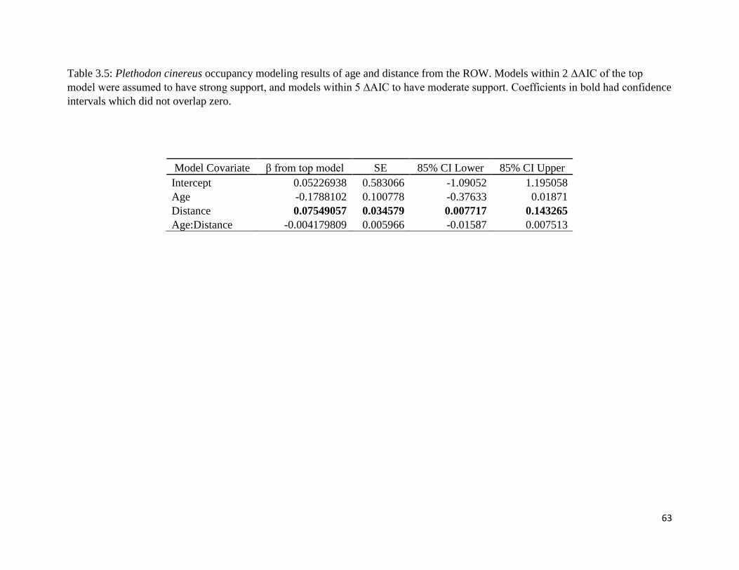
63
Table 3.5: Plethodon cinereus occupancy modeling results of age and distance from the ROW. Models within 2 ∆AIC of the top
model were assumed to have strong support, and models within 5 ∆AIC to have moderate support. Coefficients in bold had confidence
intervals which did not overlap zero.
Model Covariate β from top model SE 85% CI Lower 85% CI Upper
Intercept 0.05226938 0.583066 -1.09052 1.195058
Age -0.1788102 0.100778 -0.37633 0.01871
Distance 0.07549057 0.034579 0.007717 0.143265
Age:Distance -0.004179809 0.005966 -0.01587 0.007513

64
Chapter 4:
Variation in Pollinator Presence Along Natural Gas Pipeline Right of Ways in Northern
Appalachia

65
Formatted for submission to the Journal Biodiversity and Conservation
Variation in pollinator presence along natural gas pipeline right of ways in northern
Appalachia
Abstract
Recent global decline of pollinators has been attributed to many factors, including loss of
habitat, pollution, and agricultural use of herbicides and pesticides. The Appalachian region of
the United States has undergone forest maturation on a large scale, with few areas of grassland
and young forest habitat present on the landscape. Powerline corridors have previously been
found to positively impact pollinator populations, and I predicted that natural gas pipeline right
of ways (ROW) could serve a similar role. I examined butterfly and bee density and species
richness along natural gas pipelines that varied in age, width, vegetation structure and
composition, and seed mix used. The best predictor of butterfly richness, and bee and butterfly
density was the percentage of flowering plants. These results suggest that ROW, similar to
powerline corridors, can provide benefits to local pollinators if they are reclaimed with diverse
mixes of native plants that prioritize flower density over a grass monoculture.
Keywords: bee, butterfly, Marcellus, natural gas, pollinator, right of way, ROW

66
4.1 Introduction
Pollinator populations have shown marked declines globally over the previous decades
(Kluser and Peduzzi 2007, Rhodes 2018). Potential causes are varied, including habitat loss, use
of herbicides and pesticides in agriculture, increasing homogeneity on large-scale farms, disease,
and invasive species (Cane and Tepedino 2001). Although ecological services of pollinators are
largely focused on the non-native honey bee (Apis Spp.) and agricultural pollination, there are
many types of native pollinator insects that also provide this ecological service, among others. In
the Appalachian region of the United States, early successional habitat that provides forage
habitat for pollinators has been declining due to changes in agricultural practices, forest
maturation, and the abandonment of small-scale farms (Stauffer et al. 2018).
The Appalachian region has also seen extensive development of natural gas resources
within the last 15 years (Carter et al. 2011). Horizontal drilling technology enabled more
efficient extraction of gas from the Marcellus Shale, a deeper geologic layer than had been
previously developed (Carter et al. 2011, Zinkhan Jr. 2016). Compared with conventional
vertical wells, multiple unconventional horizontal wells can be co-located on a single well pad
(Zinkhan Jr. 2016). Along with an increase in production when utilizing hydraulic fracturing, an
unconventional well pad can produce larger volumes of natural gas than a vertical well (Carter et
al. 2011). Large gas volumes necessitate connecting wells and storage and production facilities
using pipelines.
Natural gas pipeline right of ways (ROW) must be managed to preclude the growth of
large tree roots that could negatively impact pipeline integrity. A larger body of research exists
for powerline corridors, which is a similar analogue to a pipeline ROW. Vegetation is commonly
controlled using mechanical or chemical methods to eliminate woody growth (Wagner et al.

67
2014). When these ROWs are routed through forested areas, they act as narrow corridors of early
successional habitat. While these linear ROWs can increase forest fragmentation, they can also
create habitat for pollinators and other insect species (Sheridan et al. 1997, Langlois et al. 2017,
Wagner et al. 2019). Powerline ROWs have been found to support populations of rare and
threatened pollinator species in an otherwise forested landscape (Sheridan et al. 1997).
Similarities between powerline ROWs and natural gas pipeline ROWs suggest that reclaimed
ROWs may benefit pollinators in predominately forested habitats.
This study examined pollinator diversity and density along natural gas pipeline ROWs in
Northern Pennsylvania. Pipeline ROWs varied in width, age, and seed mix used during
reclamation. I predicted that foraging habitat of butterflies is most influenced by flower diversity
and vegetation structure, and that differences in seed mixes planted during ROW reclamation
would influence pollinator presence. I also predicted that butterfly species richness would
increase as the proportion of flowering plants increased. Older ROWs should have higher
butterfly species richness than younger ROWs due to taller, denser vegetation that provides
cover and forage habitat. Variation in pollinator presence among sites informs best management
practices for creating forage habitat for pollinators on pipeline ROWs.
4.2 Methods
4.2.1 Study Site
The study area included two land parcels managed by the State of Pennsylvania: the
Tiadaghton State Forest and Game lands 12 (Figure 4.1). These state-managed land parcels are
within 100 km of the city of Williamsport and heavily forested. Average annual temperatures

68
range from 1 – 13°C, and annual precipitation is 305 cm including snowfall. The dominant forest
type is northern hardwood, with American beech (Fagus grandifolia), red maple (Acer rubrum),
black cherry (Prunus serotina) , white oak (Quercus alba) , chestnut oak (Quercus montana) ,
white pine (Pinus strobus), and eastern hemlock (Tsuga canadensis) being common. Study sites
were chosen based on the quantity of gathering pipelines present and forest cover. Pipelines were
hand digitized using publicly available National Agriculture Imagery Program (NAIP) Imagery
from 2007 to 2016 and well permit locations from the Pennsylvania Department of
Environmental Protection (PADEP 2018). The width, age, and reclamation plan for pipelines
varied within and among sites. Eighty sites were located randomly along pipelines within the
study areas (40 each on the Game lands and State Forest, respectively) and at least 500 meters
apart.
The Tiadaghton State Forest is administered by the Pennsylvania Department of
Conservation and Natural Resources (DCNR) and encompasses 59,300 hectares (Figure 4.1).
This forest is located primarily in Lycoming County with some parcels extending into
surrounding counties. Terrain includes steep mountains with cold mountain streams between
them. Much of the ground cover is forest, and regular timber harvest does occur. The ridge-tops
within the forest were primarily developed in 2012 and 2013 for natural gas extraction.
Approximately 76 km of pipeline are present on the state forest to support 42 well pads and 254
wells as of 2018.
Game lands 12 (GL12) is approximately 10,350 hectares and administered by the
Pennsylvania State Game Commission (Figure 3.1). It is located Northwest of the Tiadaghton
State Forest, and is a more contiguous patch of land. Natural Gas development did not start until
2016 within the game lands, with the most recent pipeline completed in 2019. The southern trunk

69
line is approximately 11 km long and was completed in 2016. The Northern pipeline is
approximately 18 km long and was completed in 2019. This pipeline was reclaimed with 16
different seed mixes, all of which used a diverse assemblage of native plants.
4.2.2 Sampling Protocol
Eighty survey sites were randomly located along ROWs within the study areas, divided
equally between the state forest and game lands. A modified Pollard walk was used to survey for
butterflies and other pollinators at each study site along a 100m section of ROW (Pollard and
Yates 1993). Transects were in the center of each ROW with a width of 5m on each side.
Surveys were conducted at a consistent walking pace, and all observed butterflies and bees
photographed in a passive manner without netting or handling. If species were observed but are
unable to be photographed, they were identified to the lowest level possible. Four total surveys
were conducted between May and August during 2019 and 2020 to capture heterogeneity over
time. All 80 sites were surveyed over four 2-week periods during each year, with each site at
least 10 days apart. Surveys were conducted between the hours of 09:00 and 16:00 while weather
was fair and vegetation was dry. Butterfly species richness was calculated for each site, along
with the density of butterflies and bees observed (count per transect area).
4.2.3 Pollinator Identification
Butterflies were identified to the lowest taxonomic level possible given based on
photographs. Butterflies of Pennsylvania (Monroe and Wright 2017)was the primary source for
identifying to the species level. Some species exhibit high levels of visual similarity, (e.g.,.
family Hesperiidae) and are difficult to identify without the use of a microscope. Visually
similar species were counted as a single species because of these difficulties (see Appendix H for
species groupings). Similar methods were used when photographs were of poor quality or did not

70
show distinguishing identification characteristics. Bee species, many of which exhibit
intraspecific visual heterogeneity, were not identified due to difficulties using photographs alone.
4.2.4 Survey variables
Vegetation and abiotic characteristics of the ROW were measured at each site.
Vegetation was measured during each survey within 3 randomly placed 1-m² plots. Maximum
vegetation height, the percentage of ground covered by vegetation, and the percentage of
flowering plants were measured. Measurements from each plot were averaged for each survey,
and the results of all surveys averaged for a single number for each site. ROW width and total
opening width (including a road if present) were measured using a Bushnell laser rangefinder.
ROW age obtained from pipeline environmental plans from the Pennsylvania Game Commission
and Department of Conservation and Natural Resources, and verified using National Agriculture
Imagery Program data.
4.2.5 Data Analysis
Butterfly density, butterfly species richness, and bee density were modeled separately
using a general linear model assuming a Poisson or negative binomial distribution. A Poisson
distribution was used for modeling butterfly species richness, and butterfly and bee density were
modeled using a negative binomial distribution due to overdispersion. All analyses were
performed using the program R (ver. 4.0.2) and the unmarked, AICmodAVG, and MASS
packages. Biotic and abiotic covariates were measured at each site, and the relative importance
of each tested within a model set. Models were created a priori and ranked using Akaike’s
Information Criterion for small sample sizes (AICc) (Akaike 1973). Models within 2 ∆AIC of
the top model are assumed to have considerable support, and models within 7 ∆AIC of the top
model to have moderate support (Burnham et al. 2011). Models included in analysis were all

71
covariates alone, an additive vegetation model with vegetation height, ground cover, and flower
percentage, and a full model. Modeling occupancy would have provided better resolution of site-
level changes over time, but it cannot be assumed that there is a closed population and that every
species or individual is able to be detected during each survey. The hatch dates of butterfly
species vary, and thus cannot be assumed that they are always present to be detected.
4.3 Results
4.3.1 Summary statistics
Twenty-five different species of butterfly were observed on ROWs during both field
seasons. On average, butterfly richness per site was lower in 2020 than 2019 (3.36 and 4.48,
respectively). Butterflies were observed at all sites, and bees observed at 74 of 80. The highest
butterfly species richness for a single site was 11 and the lowest 1 with a mean 2.42, while the
highest density during a survey was 18 with the lowest 0 and mean 3.38. The highest bee density
recorded from a survey was 53 with the lowest 0 and mean 5.39.
Right of Way vegetation height measurements ranged from 20.67 to 117.68cm (avg
62.2cm). Average vegetation ground cover ranged from 25 to 97.08% (avg 81.15%), and average
flower percentage ranged from 0 to 36.67% (avg. 11.78%). Flower percentage was the only
measurement that decreased over time, as some areas did not have species that flowered
throughout the field season.
4.3.2 Modeling results
Flower percentage was in all the top models when modeling butterfly species richness
(Table 4.2). Richness was predicted to increase (β = 0.028, SE = 0.007, 95% CI (0.014, 0.042))

72
as flower percentage increased (Figure 4.2). Other models with support were the vegetation
model and full model, although flower percentage was the only covariate in the top models
which did not overlap zero within 95% confidence intervals.
The top model for butterfly density included flower percentage alone (Table 4.2).
Predicted density increased (β = 0.04663244, SE = 0.006418, 95% CI (0.03405318, 0.059212))
as flower percentage increased (Figure 4.2). The vegetation and full models had some support
(within 3 ∆AIC), but all coefficients for variables apart from flower percentage overlapped zero
within confidence intervals.
Bee density modeling followed similar trends to butterfly richness and density. Flower
percentage was the top model, with the vegetation and full models having some support (Table
4.2). Density was predicted to increase (β = 0.106423, SE = 0.009901, 95% CI (0.08701704,
0.125829)) as flower percentage increased (Figure 4.2). Flower percent was the only covariate
within models with support whose estimated beta coefficient did not overlap zero within
confidence intervals.
4.4 Discussion
The most important factor that predicted pollinator richness and density in every case was
the percentage of actively flowering vegetation. This is a logical outcome and multiple studies
have found similar results (Yahner 2004, Russell et al. 2018, Wagner et al. 2019, Russo et al.
2021). Food availability of nectar provides incentive for pollinators to forage in an area. For
some species such as the monarch butterfly (Danaus plexippus) that require specific host plants,
there is no alternative location in an otherwise forested setting for those host plants to exist

73
besides areas of timber harvest or ROWs (Thogmartin et al. 2017). ROWs have been found to
increase butterfly diversity and abundance in forested landscapes regardless of surrounding
landcover type, likely due to specialist needs of some species (Berg et al. 2016).
Contrary to my predictions, neither ROW age nor width were supported predictors of
density during modeling, although it is expected that pollinator numbers would increase as width
increases. Since surveys on transects did not record all pollinators seen on the ROW, but only
those within the 10m width of the transect. Consequently, the total number of pollinators on a
ROW is based on the total number of flowers present, regardless of other factors. Pollinator
species richness and abundance have been found to be positively related with flower abundance
(Russell et al. 2005, Eldegard et al. 2017b, Roberts et al. 2017). Poor support for age is most
likely a result of large variation of flower percent along ROWs. Many older ROWs were nearly
grass monocultures, which failed to produce food resources of nectar that would attract
pollinators (Figure 4.3). Vegetation structure was on average taller and denser on older ROWs,
and bee abundance has been linked to vegetation height (Roberts et al. 2017). The type of
vegetation management was not examined in this study, but more frequent management has been
found to promote diversity over non-managed fields (Eldegard et al. 2017b).
A factor that was not investigated in this study was change in flower cover over time.
Anecdotally, there were sites where flower percentage changed drastically between visits. At
sites where clover was the dominant species, flowers were only present during one or two
surveys per year, but no flowers were present during the final survey. Sites that are planted to
produce flowers throughout the growing season have been found to increase pollinator numbers
(Eldegard et al. 2017b, Wagner et al. 2019).

74
The results of this study show that the percentage of flowering plants on a ROW is the
most influential factor in predicting pollinator density. The seed mixes planted on the youngest
ROW (north-western most pipeline on the Game Lands 12 site) featured a diverse mix of annual
and perennial forbs and grasses (Appendix G). The majority of these mixes were comprised of
species that flowered in the mid or late season, which may be why pollinator observations were
higher during those time periods. Sample sizes of sites were too small for comparison of
effectiveness of each seed mix, and vegetation composition of each site will likely change over
time as the perennial species become more established and mature. Additional study of these
seed mixes over time and a more thorough examination of diversity is recommended. Overall,
seed mixes should be chosen to provide as many flowers as possible for the longest duration of
time. Choosing plant species that have asynchronous flowering cycles will extend the time that
pollen and nectar food resources are available to pollinators. When there is the option, native
plants should be prioritized over ornamentals and non-natives, as linear infrastructure has been
found to increase invasive plant expansion (Barlow et al. 2017).
The only negative associated with a diverse and robust seed mix planting during
reclamation is cost. It is easier for reclamation to only use one type of grass seed (the most
commonly encountered monoculture on sites in this study) than to deal with 17 different mixes
and worry about potential germination and soil erosion issues. Specialty native seeds and
producing mixes are also much more expensive. In an ecological sense, there is no downside to
creating a field analogue with a diverse mix of native flowering plants on a pipeline ROW. A
ROW that is a grass monoculture provides no benefit to most types of wildlife or pollinators
(Wagner et al. 2019). In forested areas that are already being negatively impacted by pipeline

75
infrastructure (fragmentation and edge effects), reclaiming ROWs with high quality seed mixes
provides a benefit for pollinators at no additional ecological cost.
76
Literature cited
Akaike, H. 1973. Information theory as an extension of the maximum likelihood principle. Pages
267–281 in. Second International Symposium on Informantion Theory, Akademiai Kiado,
Budapest.
Barlow, K. M., D. A. Mortensen, P. J. Drohan, and K. M. Averill. 2017. Unconventional gas
development facilitates plant invasions. Journal of Environmental Management 202:208–
216. Elsevier Ltd. <http://dx.doi.org/10.1016/j.jenvman.2017.07.005>.
Berg, Å., K. O. Bergman, J. Wissman, M. Żmihorski, and E. Öckinger. 2016. Power-line
corridors as source habitat for butterflies in forest landscapes. Biological Conservation
201:320–326.
Burnham, K. P., D. R. Anderson, and K. P. Huyvaert. 2011. AIC model selection and
multimodel inference in behavioral ecology: Some background, observations, and
comparisons. Behavioral Ecology and Sociobiology 65:23–35.
Cane, J. H., and V. J. Tepedino. 2001. Causes and extent of declines among native North
American invertebrate pollinators: Detection, evidence, and consequences. Ecology and
Society 5.
Carter, K. M., J. A. Harper, K. W. Schmid, and J. Kostelnik. 2011. Unconventional natural gas
resources in Pennsylvania: The backstory of the modern Marcellus Shale play.
Environmental Geosciences 18:217–257.
Eldegard, K., D. L. Eyitayo, M. H. Lie, and S. R. Moe. 2017. Can powerline clearings be
managed to promote insect-pollinated plants and species associated with semi-natural
grasslands? Landscape and Urban Planning 167:419–428. Elsevier.
<http://dx.doi.org/10.1016/j.landurbplan.2017.07.017>.
Kluser, S., and P. Peduzzi. 2007. Global Pollinator Decline : A Literature Review’.
Langlois, L. A., P. J. Drohan, and M. C. Brittingham. 2017. Linear infrastructure drives habitat
conversion and forest fragmentation associated with Marcellus shale gas development in a
forested landscape. Journal of Environmental Management 197:167–176. Elsevier Ltd.
<http://dx.doi.org/10.1016/j.jenvman.2017.03.045>.
Monroe, J. L., and D. M. Wright. 2017. Butterflies of Pennsylvania: a field guide. University of
Pittsburgh Press, Pittsburgh.
PADEP. 2018. Issued Gas Well Permits. Pennsylvania Department of Environmental Protection.
<http://www.depreportingservices.state.pa.us/ReportServer/Pages/ReportViewer.aspx?/Oil_
Gas/Permits_Issued_Detail>.
Pollard, E., and T. Yates. 1993. Monitoring Butterflies for Ecology and Conservation. Chapman
& Hall, London, UK.
Rhodes, C. J. 2018. Pollinator decline – An ecological calamity in the making? Science Progress
101:121–160.
Roberts, H. P., D. I. King, and J. Milam. 2017. Factors affecting bee communities in forest

77
openings and adjacent mature forest. Forest Ecology and Management 394:111–122.
Elsevier B.V. <http://dx.doi.org/10.1016/j.foreco.2017.03.027>.
Russell, K. N., H. Ikerd, and S. Droege. 2005. The potential conservation value of unmowed
powerline strips for native bees. Biological Conservation 124:133–148.
Russell, K. N., G. J. Russell, K. L. Kaplan, S. Mian, and S. Kornbluth. 2018. Increasing the
conservation value of powerline corridors for wild bees through vegetation management: an
experimental approach. Biodiversity and Conservation 27:2541–2565. Springer
Netherlands. <https://doi.org/10.1007/s10531-018-1552-8>.
Russo, L., H. Stout, D. Roberts, B. D. Ross, and C. G. Mahan. 2021. Powerline right-of-way
management and flower-visiting insects : How vegetation management can promote
pollinator diversity. PLoS ONE 1–17. <http://dx.doi.org/10.1371/journal.pone.0245146>.
Sheridan, P. M., S. L. Orzell, and E. L. Bridges. 1997. Powerline easements as refugia for state
rare seepage and pineland plant taxa. Sixth International Symposium on Environmental
Concerns in Rights-of-Way Management. JR Williams, JW Goodrich-Mahoney, JR
Wisniewski, and J. Wisniewski, editors. Elsevier Science, Oxford, England 451–460.
<http://www.pitcherplant.org/Papers/powerlineeasements.htm>.
Stauffer, G. E., D. A. W. Miller, L. M. Williams, and J. Brown. 2018. Ruffed grouse population
declines after introduction of West Nile virus. Journal of Wildlife Management 82:165–172.
Thogmartin, W. E., R. Wiederholt, K. Oberhauser, R. G. Drum, J. E. Diffendorfer, S. Altizer, O.
R. Taylor, J. Pleasants, D. Semmens, B. Semmens, R. Erickson, K. Libby, and L. Lopez-
Hoffman. 2017. Monarch butterfly population decline in north america: Identifying the
threatening processes. Royal Society Open Science 4.
Wagner, D. L., K. J. Metzler, and H. Frye. 2019. Importance of transmission line corridors for
conservation of native bees and other wildlife. Biological Conservation 235:147–156.
Elsevier. <https://doi.org/10.1016/j.biocon.2019.03.042>.
Wagner, D. L., K. J. Metzler, S. A. Leicht-Young, and G. Motzkin. 2014. Vegetation
composition along a New England transmission line corridor and its implications for other
trophic levels. Forest Ecology and Management 327:231–239. Elsevier B.V.
<http://dx.doi.org/10.1016/j.foreco.2014.04.026>.
Yahner, R. H. 2004. Wildlife Response to More Than 50 Years of Vegetation Maintenance on a
Pennsylvania, U.S., Right-of-Way. Journal of Arboriculture 30:123–126.
Zinkhan Jr., F. 2016. Site Characteristics Associated with Conventional and Unconventional
Petroleum Development in West Virginia. West Virginia University.

78
Figure 4.1: Location of main study sites in Pennsylvania (A). Site B is the Tiadaghton State
Forest while C is PA state game lands 12. Study sites located on Pennsylvania Game
Commission game lands 12. 80 sample sites are evenly distributed between A and B. All
pipelines in the Tiadaghton State Forest were constructed in 2013. There are 2 pipelines within
the game lands site, the northern line completed in 2019 and the southern line completed in 2017

79
Figure 4.2 Predicted butterfly species richness, butterfly density, and bee density based on the
percentage of flowers present on a natural gas pipeline ROW. Flower percentage was the best
supported predictor for all pollinator metrics when modeled against ground cover, vegetation
height, ROW age, and ROW width.

80
Figure 4.3: An example of natural gas pipeline right of ways (ROW) with large differences in
flower percentage due to seed mix choice during reclamation. The ROW above had higher
pollinator richness and density than the ROW below.

81
Table 4.1: Covariates included in modeling to predict pollinator richness and density on a
pipeline right of way (ROW) in Pennsylvania. Model sets tested included all covariates
individually, a vegetation model with vegetation height, ground cover, and flower percentage,
and a full model.
Covariate Description
Vegetation Height Maximum height of vegetation along ROW
Ground Cover Percent of ROW covered with vegetation
Flower Percentage of plants flowering at time of survey
Age Years since ROW reclamation
ROW Width Width of ROW

82
Table 4.2 Modeling results for butterfly richness, butterfly density, and bee density along natural gas
pipeline ROWs in Pennsylvania. Model support was ranked using AICc, with top models assumed to be
within 2 ∆AICc of the top model. Models within 7 ∆AICc are assumed to have some support. A Poisson
distribution was used for butterfly richness, and a negative binomial distribution used for butterfly and
bee density due to overdispersion.
Butterfly richness
Model covariates AICc ∆AIC ω
Veg Height + Ground Cover + Flower 288.97 0 0.48
Flower 289.75 0.78 0.32
Full Model 290.77 1.8 0.19
Null 302.93 13.96 0
Vegetation Height 303.13 14.16 0
Age 304.66 15.69 0
Ground Cover 304.94 15.97 0
ROW Width 305.01 16.05 0
Age + ROW Width 306.64 17.67 0
Butterfly count
Model covariates AICc ∆AICc ω
Flower 499.43 0 0.61
Veg Height + Ground Cover + Flower 501.88 2.08 0.21
Full 537.8 2.45 0.18
Age 538.01 38.36 0
Null 538.06 38.57 0
Ground Cover 538.91 38.63 0
ROW Width 539.69 39.48 0
Vegetation Height 539.69 40.26 0
Age + ROW Width 539.76 40.33 0
Bee count
Model covariates AIC ∆AIC ω
Flower 475.53 0 0.83
Veg Height + Ground Cover + Flower 478.93 3.4 0.15
Full 482.93 7.4 0.02
Ground Cover 537.14 61.61 0
Null 543.22 67.69 0
Vegetation Height 543.28 67.75 0
ROW Width 544.77 69.24 0
Age 545.37 69.84 0
Age + ROW Width 546.69 71.16 0

83
Chapter 5
Management Implications

84
5. Management Implications
5.1 Game birds and large mammals
The low number of ruffed grouse (Bonasa umbellus) observed during surveys make it
difficult to make any meaningful recommendations for pipeline ROW reclamation. In both study
sites (Tiadaghton State Forest and Game Lands 12), actions were being performed to improve
nesting habitat and cover for ruffed grouse. In Game Lands 12, multiple areas of 4–5 acres had
been clear cut with the intention of improving grouse habitat, and this was done using funds
received for the most recent pipeline construction on the property. I expect that these areas will
provide better nesting habitat and vertical cover for grouse (Whitaker and Stauffer 2004, Felix-
Locher and Campa 2010). I also predict that ROWs can provide foraging habitat for broods, as
grassland-type vegetation has been found to have larger insect and arthropod populations than
open forest (Haulton 1999, Haulton et al. 2003). The number of eastern wild turkeys (Meleagris
gallopavo) observed while traveling along pipelines can act as some evidence that they are useful
to ground birds for foraging habitat (see figure 1). White-tailed deer (Odocoileus virginianus)
were also seen foraging often while traveling along pipelines, and variation existed between
study sites. Higher quality seed mixes on the Game Lands may be contributing to this difference,
but further research is required to fully test this hypothesis. Previous work has been done on
using warm season grasses in food plots, and the potential benefits for areas over-browsed by
deer (Hehman and Fulbright 1997, Lashley et al. 2011).
5.2 Salamanders and Snakes
Eastern red backed salamanders (Plethodon cinereus) were less likely to be found on
ROWs than in interior forest, which is consistent with previous work done on forest-dwelling
terrestrial salamanders and forest fragmentation (Marsh and Beckman 2004, Marsh et al. 2005).

85
The best predictor of salamander presence was the distance of cover boards from the center of
the ROW, with occupancy probability increasing as distance increased. It is unlikely that the loss
of habitat from a pipeline will have lasting effects on local populations, but there is a potential to
segregate populations with new road construction. There is literature that shows roads as a
barrier to population connectivity, but also shows terrestrial salamanders are capable of
dispersing across open fields larger than the ROWs in this study (Marsh et al. 2004, 2005).
Reintroducing coarse woody debris to ROWs following reclamation would benefit local
salamander populations and other amphibians by providing cover. Salamanders were found to
utilize coarse woody debris on powerline sites (Brannon et al. 2014).
Snakes were much more likely to occupy sites on the ROW than off it, in contrast to
salamanders. Snakes often utilize edge habitat, and likely prefer ROWs for increased food
density and higher solar radiation for improved thermoregulation. High prevalence of meadow
voles (Microtus pennsylvanicus) and nests under coverboards on the ROW suggests that these
areas provide ample food resources for larger rattlesnakes. Combined with rock structure
creation, I anticipate that ROWs in the study area may be beneficial to local timber rattlesnake
populations by providing food resources and hibernacula. It is possible, however, that increased
heavy truck traffic and recreational traffic (due to improved roads during pipeline construction)
may lead to higher road mortality and human-caused persecution of this species, but this would
need to be studied in more detail to provide a definitive answer. In one study, human caused
mortality and vehicle strikes were the second and third most common cause of death for timber
rattlesnakes behind predation (Olson et al. 2015).

86
5.3 Pollinators
Pollinator density and species richness was positively correlated with the
percentage of flowering plants present. These findings are consistent with previous work
measuring pollinators on utility ROWs (Berg et al. 2016, Eldegard et al. 2017a, Russo et al.
2021). Choosing seed mixes that prioritize flowering plants with different flowering schedules to
maximize the extent of flower presence throughout the growing season will provide the best
benefits to local pollinator populations. There was no interactive effect found between pollinator
density and overall ROW width, suggesting that there is a linear relationship between pollinator
abundance and habitat size. I expect that pollinator abundance will increase as the amount of
flowers increases, meaning that pollinator abundance will be higher on wider ROWs assuming
the percentage of flowering plants is the same.
5.4 Overall Recommendations
To provide the best benefit to wildlife, the results of this study indicate that prioritizing
ROW siting along existing roads, along established early successional vegetation or within areas
of young forest habitat. Natural gas pipeline ROWs in a forested setting will negatively impact
terrestrial salamanders, but limiting new pipelines to existing roads or young forest will
minimize these effects. A more costly approach would be to utilize horizontal directional drilling
to created alternating patches of grassland and undisturbed forest over the pipeline (Allouche et
al. 2000). Seed mixes used during reclamation should be chosen to maximize the number of
flowers present throughout the growing season with warm and cool season grasses to provide
structure and forage for larval pollinators (Figures 5.2, 5.3). Seed mixes should also include only
native species, and care taken to deter the introduction or expansion of any invasive plant
species. The temporary workspace of the ROW can be replanted with fruiting native trees and

87
shrubs which will provide food resources for wildlife species and reduce edge effects on (Figure
5.4). Rock structures located along ROW edges can also be created to provide hibernacula for
snakes (Figure 5.5). Siting and reclamation of pipelines that follow these recommendations will
provide benefits to wildlife and limit the negative effects that forest fragmentation has on others.
Right of way width negatively effects salamanders, but is beneficial to pollinators assuming a
quality seed mix is used. This highlights the anachronism of a ROW in a forested landscape;
some species will benefit and others suffer regardless of ROW location or reclamation. It is up to
the local land manager to determine prioritization of species’ needs.
88
Literature cited
Allouche, E. N., S. T. Araratnam, and J. S. Lueke. 2000. Horizontal Directional Drilling: Profile
of an Emerging Industry. Journal of Construction Engineering and Management 126:68–76.
Berg, Å., K. O. Bergman, J. Wissman, M. Żmihorski, and E. Öckinger. 2016. Power-line
corridors as source habitat for butterflies in forest landscapes. Biological Conservation
201:320–326.
Brannon, P., E. C. Allan, and M. C. Silinski. 2014. Terrestrial Salamander Abundances Along
and Within an Electric Power Line Right-of-Way. Journal of the North Carolina Academy
of Science 132:40–45.
Eldegard, K., D. L. Eyitayo, M. H. Lie, and S. R. Moe. 2017. Can powerline clearings be
managed to promote insect-pollinated plants and species associated with semi-natural
grasslands? Landscape and Urban Planning 167:419–428. Elsevier.
<http://dx.doi.org/10.1016/j.landurbplan.2017.07.017>.
Felix-Locher, A., and H. Campa. 2010. Importance of habitat type classifications for predicting
ruffed grouse use of areas for drumming. Forest Ecology and Management 259:1464–1471.
Elsevier B.V. <http://dx.doi.org/10.1016/j.foreco.2010.01.020>.
Haulton, G. S. 1999. Ruffed Grouse Natality, Chick Survival, and Brood Micro-Habitat
Selection in the Southern Appalachians. Virginia Polytechnic Institute and State University.
Haulton, G. S., F. Stauffer, R. L. Kirkpatrick, and G. W. Norman. 2003. Ruffed Grouse ( Bonasa
umbellus ) Brood Microhabitat Selection in the Southern Appalachians. The American
Midland Naturalist 150:95–103.
Hehman, M. W., and T. E. Fulbright. 1997. Use of Warm-Season Food Plots by White-Tailed
Deer. The Journal of Wildlife Management 61:1108–1115.
Lashley, M. A., C. A. Harper, G. E. Bates, and P. D. Keyser. 2011. Forage availability for white-
tailed deer following silvicultural treatments in hardwood forests. Journal of Wildlife
Management 75:1467–1476.
Marsh, D. M., and N. G. Beckman. 2004. Effects of forest roads on the abundance and activity of
terrestrial salamanders. Ecological Applications 14:1882–1891.
Marsh, D. M., G. S. Milam, N. P. Gorham, and N. G. Beckman. 2005. Forest roads as partial
barriers to terrestrial salamander movement. Conservation Biology 19:2004–2008.
Marsh, D. M., K. A. Thakur, K. C. Bulka, and L. B. Clarke. 2004. Dispersal and colonization
through open fields by a terrestrial, woodland salamander. Ecology 85:3396–3405.
Olson, Z. H., B. J. MacGowan, M. T. Hamilton, A. F. T. Currylow, and R. N. Williams. 2015.
Survival of Timber Rattlesnakes (Crotalus horridus): Investigating Individual,
Environmental, and Ecological Effects. Herpetologica 71:274–279.
Russo, L., H. Stout, D. Roberts, B. D. Ross, and C. G. Mahan. 2021. Powerline right-of-way
management and flower-visiting insects : How vegetation management can promote
pollinator diversity. PLoS ONE 1–17. <http://dx.doi.org/10.1371/journal.pone.0245146>.

89
Whitaker, D. M., and D. F. Stauffer. 2004. Ruffed grouse (Bonasa umbellus) habitat ecology in
the central and southern Appalachians. ProQuest Dissertations and Theses 220 p.
<http://ezproxy.usherbrooke.ca/login?url=http://search.proquest.com/docview/305105487?a
ccountid=13835 L2 - http://sfxhosted.exlibrisgroup.com/sherbrooke?url_ver=Z39.88-
2004&rft_val_fmt=info:ofi/fmt:kev:mtx:dissertation&genre=dissertations+%26+theses&sid
=P>.

90
Figure 5.1: Eastern wild turkey (Meleagris gallopavo) hen observed on a pipeline ROW.
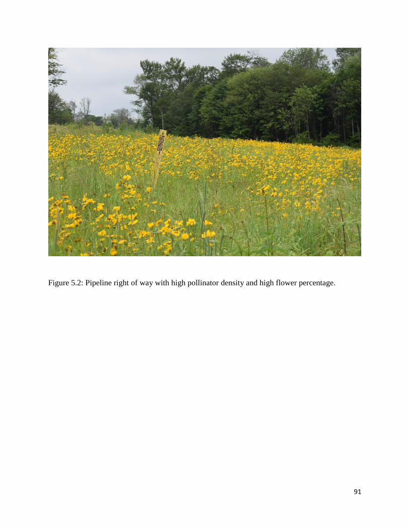
91
Figure 5.2: Pipeline right of way with high pollinator density and high flower percentage.

92
Figure 5.3 Pipeline right of way on the Tiadaghton State Forest with low pollinator density, poor
vegetation diversity, and no flower growth.

93
Figure 5.4: An example of a natural gas pipeline ROW temporary workspace that has been
replanted with trees and shrubs, and the pipeline routed along an existing road. The pipeline is
positioned in line with the yellow marker, visible in the center right portion of the photograph.

94
Figure 5.5 Example of a rock structure constructed along a natural gas pipeline ROW to provide
hibernacula for snakes.

95
Appendix A: Study site locations, ROW Age (years, ROW width (in metes, with and without a
road), and seed mix of each site (sites 4A – 30A).
ID UTME UTMN Age
Total ROW
width
ROW
Width Road
seed
mix
1A 356428 4604740 3 30 30 0 2A 356422 4605152 3 33 12 1 3A 356741 4605596 3 26 11 1 4A 349660 4605727 1 32 32 0 1
5A 349869 4606190 1 30 30 0 1
6A 350507 4606131 1 41 25 1 1
7A 351436 4606172 1 35 28 1 3
8A 351912 4606467 1 35 26 1 5
9A 352335 4606800 1 35 18 1 13
10A 352672 4607171 1 32 23 1 9
11A 353033 4607568 1 40 16 1 15
12A 353398 4607588 1 28 19 1 15
13A 353686 4607176 1 38 38 0 16
14A 354183 4607236 1 28 16 1 6
15A 354419 4607720 1 42 24 1 15
16A 354571 4608269 1 34 26 1 15
17A 354872 4608640 1 38 26 1 3
18A 355292 4608945 1 33 17 1 9
19A 355721 4608627 1 38 25 1 3
20A 356081 4608689 1 34 18 1 6
21A 356636 4608803 1 36 25 1 5
22A 356926 4609246 1 35 22 1 6
23A 357230 4609733 1 41 21 1 2
24A 357238 4610151 1 25 10 1 6
25A 357393 4610620 1 115 115 0 2
26A 358117 4611077 1 30 30 0 16
27A 358398 4611525 1 44 29 1 3
28A 358889 4612409 1 33 33 0 7
29A 359252 4612699 1 37 37 0 2
30A 360116 4613211 1 46 32 1 10
31A 357907 4605468 3 27 11 1 32A 357385 4605223 3 26 12 1 33A 357007 4604933 3 25 13 1 34A 358275 4605777 3 28 16 1 35A 358638 4605611 3 29 11 1 36A 359210 4605677 3 25 11 1

96
37A 359692 4605510 3 35 20 1 38A 360209 4605762 3 30 20 1 39A 360639 4605599 3 27 18 1 40A 361182 4605679 3 28 18 1 1B 298097 4572270 7 30 11 1 2B 299732 4573050 7 26 12 1 3B 299839 4573440 7 17 13 1 4B 301582 4572370 7 16 10 1 5B 300393 4572670 7 16 10 1 6B 302391 4573040 7 22 10 1 7B 296642 4573450 7 20 13 1 8B 297949 4573790 7 32 12 1 9B 298141 4574360 7 27 15 1 10B 295483 4574400 7 23 13 1 11B 295945 4574790 7 30 18 1 12B 300153 4574110 7 17 11 1 13B 300309 4574880 7 18 10 1 14B 298562 4575520 7 24 14 1 17B 304330 4576785 7 35 24 1 18B 303886 4575300 7 25 14 1 19B 305415 4576660 7 21 12 1 20B 303296 4576920 7 20 20 0 21B 306736 4576720 7 25 16 1 22B 301313 4577665 7 34 13 1 23B 301215 4578320 7 45 45 0 24B 304259 4579140 7 24 10 1 25B 305124 4579120 7 25 10 1 26B 306364 4578420 7 24 17 1 27B 300880 4579960 7 25 17 1 28B 291613 4581120 7 34 18 1 29B 290853 4581270 7 20 20 0 30B 304770 4579830 7 25 10 1 31B 301379 4580170 7 22 13 1 32B 300817 4580412 7 26 14 1 33B 300368 4581057 7 28 15 1 34B 300252 4581820 7 26 21 1 35B 300844 4582680 7 33 16 1 36B 300640 4583590 7 33 18 1 37B 300412 4584480 7 24 14 1 38B 300265 4585300 7 26 15 1 39B 300924 4585680 7 38 12 1

97
40B 301563 4585930 7 25 13 1 41B 302140 4586510 7 26 16 1 42B 300459 4586600 7 26 15 1

98
Appendix B: Survey date and time for ruffed grouse, cover board searches for salamanders and snakes,
and pollinators. Ruffed grouse observations are also included for each survey (0 – not observed, 1 –
observed). Start time of surveys is using a 24 hour clock, and duration is in minutes.
Grouse Survey Herp Survey Pollinator Survey
Site Survey Date Start Duration Grouse Obs Start Duration Start Duration
1a 1 5/21/2019 9:05 7 0 9:12 8
2 6/21/2019 9:20 8 0 9:28 12
3 7/5/2019 9:23 7 0 9:30 13
4 7/22/2019 14:45 9 0 9:06 17
2a 1 5/23/2019 9:25 9 0 9:34 7
2 6/19/2019 10:08 7 0 10:15 15
3 7/8/2019 9:50 9 0 9:59 12
4 7/29/2019 9:30 8 0 9:38 13
3a 1 5/23/2019 9:43 6 0 9:49 13
2 6/10/2019 9:01 8 0 9:09 14
3 7/5/2019 9:54 8 0 10:02 16
4 7/25/2019 10:00 8 0 10:08 17
4a 1 5/21/2019 11:10 6 0 11:16 15
2 6/20/2019 9:10 8 0 9:18 12
3 7/8/2019 12:31 7 0 12:38 13
4 7/29/2019 13:30 7 0 13:37 14
5a 1 5/23/2019 11:01 10 0 11:11 13
2 6/19/2019 11:40 5 0 11:45 15
3 7/1/2019 9:10 8 0 9:18 12
4 7/22/2019 12:30 9 0 14:00 15
6a 1 5/22/2019 8:19 6 0 11:20 12
2 6/10/2019 10:01 7 0 10:08 12
3 7/3/2019 10:45 7 0 10:52 14
4 7/25/2019 11:40 8 0 11:48 15
7a 1 5/31/2019 11:59 9 0 12:08 20
2 6/19/2019 12:14 6 0 12:20 15
3 7/5/2019 13:58 8 0 14:06 16
4 7/26/2019 7:46 9 0 9:59 11
8a 1 5/24/2019 7:55 10 0 11:35 15
2 6/10/2019 8:53 9 0 9:02 12
3 7/3/2019 11:21 8 0 11:29 14
4 7/26/2019 8:33 9 0 9:46 13
9a 1 5/31/2019 11:10 10 0 11:20 14
2 6/20/2019 10:10 8 0 10:18 12
3 7/8/2019 15:39 7 0 15:46 14

99
4 7/30/2019 9:10 6 0 9:16 15
10a 1 5/31/2019 10:35 7 0 10:42 16
2 6/20/2019 10:40 6 0 10:46 14
3 7/1/2019 9:49 10 0 9:59 14
4 7/25/2019 12:23 7 0 12:30 15
11a 1 5/21/2019 10:18 10 0 10:30 12
2 6/28/2019 16:35 7 0 16:42 18
3 7/5/2019 13:21 6 1 13:27 13
4 7/25/2019 13:21 8 0 13:29 17
12a 1 5/24/2019 8:18 8 0 11:20 15
2 6/20/2019 11:12 8 0 11:20 14
3 7/3/2019 12:34 6 0 12:40 13
4 7/26/2019 8:58 7 0 9:05 18
13a 1 5/23/2019 11:35 6 0 11:41 9
2 6/20/2019 12:00 7 0 12:07 13
3 7/1/2019 10:34 7 0 10:41 17
4 7/22/2019 8:10 9 0 9:40 12
14a 1 5/23/2019 12:05 7 0 12:12 9
2 6/20/2019 12:32 6 0 12:38 14
3 7/5/2019 12:52 6 0 12:58 12
4 7/22/2019 8:37 10 0 9:56 9
15a 1 5/24/2019 8:44 8 0 8:55 15
2 6/19/2019 12:58 7 0 13:05 12
3 7/3/2019 13:06 6 0 13:12 9
4 7/25/2019 14:06 10 0 14:16 16
16a 1 5/22/2019 9:05 10 0 9:15 14
2 6/19/2019 13:30 8 0 13:38 14
3 7/8/2019 14:58 5 0 15:03 12
4 7/30/2019 10:10 5 0 10:15 15
17a 1 5/21/2019 9:43 8 0 11:48 18
2 6/19/2019 14:10 6 0 14:16 14
3 7/3/2019 13:40 6 0 13:46 14
4 7/25/2019 14:39 7 0 14:46 12
18a 1 5/24/2019 9:30 8 0 9:38 13
2 6/10/2019 10:34 8 0 10:42 18
3 7/10/2019 8:21 8 0 11:38 16
4 7/30/2019 10:40 7 0 10:47 13
19a 1 5/31/2019 9:58 10 0 10:08 14
2 6/20/2019 13:08 6 0 13:14 16
3 7/10/2019 8:58 12 0 11:16 13
4 7/30/2019 11:05 6 0 11:11 16

100
20a 1 5/21/2019 8:25 6 0 12:14 16
2 6/18/2019 16:01 5 0 16:06 14
3 7/1/2019 11:24 6 0 11:30 13
4 7/22/2019 10:46 8 0 11:31 9
21a 1 5/24/2019 10:05 7 0 10:12 10
2 6/10/2019 12:34 7 0 12:41 10
3 7/8/2019 14:20 6 0 14:26 14
4 7/30/2019 11:43 7 0 11:50 13
22a 1 5/22/2019 9:50 8 0 9:58 11
2 6/18/2019 15:29 6 0 15:35 15
3 7/3/2019 14:20 8 0 14:28 14
4 7/26/2019 11:38 8 0 11:46 14
23a 1 5/22/2019 10:20 5 0 10:25 9
2 6/10/2019 9:26 6 0 9:34 11
3 7/5/2019 12:21 7 0 12:28 12
4 7/22/2019 11:21 9 0 12:08 15
24a 1 5/24/2019 10:35 7 0 10:45 15
2 6/20/2019 13:58 8 0 14:06 18
3 7/8/2019 13:40 6 0 13:46 14
4 7/30/2019 12:30 8 0 12:38 13
25a 1 5/23/2019 12:35 7 0 12:42 9
2 6/18/2019 15:00 6 0 15:06 13
3 7/1/2019 12:00 8 0 12:08 12
4 7/26/2019 11:03 9 1 11:12 15
26a 1 5/23/2019 14:50 6 0 14:56 15
2 6/18/2019 14:30 6 0 14:36 14
3 7/1/2019 12:42 8 0 12:50 15
4 7/26/2019 10:34 7 0 10:41 17
27a 1 5/21/2019 8:59 6 0 12:40 13
2 6/18/2019 14:00 5 0 14:05 12
3 7/10/2019 9:34 8 0 9:42 14
4 7/30/2019 13:04 6 0 13:10 12
28a 1 5/22/2019 10:50 11 0 11:01 9
2 6/10/2019 11:26 9 0 11:35 15
3 7/10/2019 10:21 8 0 10:29 15
4 7/30/2019 13:34 7 0 13:41 15
29a 1 5/23/2019 15:30 8 0 15:40 13
2 6/18/2019 13:28 6 0 13:34 16
3 7/1/2019 13:26 8 0 13:34 16
4 7/25/2019 15:27 7 0 15:34 15
30a 1 5/31/2019 9:11 7 0 9:18 12

101
2 6/18/2019 13:00 8 0 13:08 12
3 7/1/2019 14:12 8 0 14:20 14
4 7/25/2019 16:03 8 0 16:11 14
31a 1 5/21/2019 14:25 9 0 14:34 16
2 6/21/2019 9:50 7 0 9:57 13
3 7/10/2019 12:49 7 0 12:56 16
4 7/29/2019 10:42 6 0 12:42 11
32a 1 5/31/2019 14:20 6 0 14:26 15
2 6/19/2019 9:01 9 0 9:10 14
3 7/8/2019 10:49 9 0 10:58 18
4 7/29/2019 10:05 6 0 10:11 17
33a 1 5/21/2019 15:10 9 0 15:19 11
2 6/19/2019 9:36 6 0 9:42 14
3 7/3/2019 9:52 8 0 10:00 12
4 7/25/2019 9:27 8 0 9:35 15
34a 1 5/22/2019 12:30 8 0 12:38 17
2 6/21/2019 10:18 6 0 10:24 16
3 7/8/2019 11:31 7 0 11:38 14
4 7/29/2019 10:34 6 0 10:40 16
35a 1 5/21/2019 13:48 7 0 13:55 14
2 6/21/2019 10:52 8 0 11:00 15
3 7/5/2019 10:36 7 0 10:43 17
4 7/22/2019 14:05 10 0 11:11 14
36a 1 5/31/2019 13:42 7 0 13:49 17
2 6/21/2019 11:30 8 0 11:38 14
3 7/10/2019 13:21 8 0 13:29 17
4 7/29/2019 11:22 6 0 11:28 16
37a 1 5/23/2019 8:35 8 0 10:11 12
2 6/21/2019 12:06 8 0 12:14 16
3 7/10/2019 14:06 6 0 14:12 14
4 7/29/2019 11:54 6 0 12:00 16
38a 1 5/31/2019 13:09 8 0 13:17 13
2 6/21/2019 13:02 6 0 13:08 16
3 7/5/2019 11:16 7 0 11:23 12
4 7/22/2019 13:36 9 0 12:19 13
39a 1 5/22/2019 13:20 6 0 13:26 12
2 6/10/2019 9:41 6 0 9:47 13
3 7/3/2019 9:02 10 0 9:12 12
4 7/25/2019 8:46 9 0 10:33 15
40a 1 5/22/2019 13:52 7 0 13:59 13
2 6/21/2019 13:48 9 0 13:57 19

102
3 7/10/2019 14:59 8 0 15:08 15
4 7/29/2019 12:40 6 0 12:46 14
1b 1 5/28/2019 14:36 8 0 14:44 13
2 6/17/2019 11:26 8 0 11:34 16
3 7/11/2019 8:14 7 0 11:30 15
4 7/31/2019 9:26 6 0 9:32 16
2b 1 5/27/2019 10:50 10 0 11:00 11
2 6/14/2019 10:48 8 0 10:56 14
3 7/11/2019 8:48 8 0 10:41 14
4 7/31/2019 10:23 7 0 10:30 12
3b 1 5/30/2019 13:59 9 0 14:08 16
2 6/14/2019 11:21 7 0 11:28 16
3 7/12/2019 9:22 9 0 9:38 11
4 7/31/2019 10:50 6 0 10:56 14
4b 1 5/26/2019 8:25 9 0 9:28 12
2 6/11/2019 9:22 8 0 9:30 18
3 7/11/2019 11:17 8 0 11:00 17
4 7/31/2019 9:55 6 0 10:01 13
5b 1 5/27/2019 10:20 10 0 10:30 16
2 6/12/2019 12:34 6 0 12:40 12
3 7/2/2019 10:42 8 0 10:50 15
4 7/23/2019 10:46 8 0 10:54 19
6b 1 5/26/2019 9:00 8 0 9:08 14
2 6/12/2019 13:06 7 0 13:13 12
3 7/2/2019 11:21 5 0 11:26 14
4 7/23/2019 11:38 6 0 11:44 16
7b 1 5/27/2019 9:22 9 0 9:31 13
2 6/14/2019 12:45 7 0 12:52 13
3 7/2/2019 12:02 8 0 11:40 16
4 7/24/2019 14:56 8 0 15:04 16
8b 1 5/26/2019 10:10 8 0 10:18 16
2 6/17/2019 12:15 7 0 12:22 13
3 7/2/2019 13:46 8 0 13:54 12
4 7/24/2019 14:16 6 0 14:22 15
9b 1 5/28/2019 15:11 7 0 15:18 17
2 6/14/2019 13:14 6 0 13:20 16
3 7/2/2019 12:08 6 0 12:14 16
4 7/24/2019 13:42 8 0 13:50 15
10b 1 5/26/2019 10:58 8 0 11:06 10
2 6/12/2019 14:44 8 0 14:52 13
3 7/11/2019 13:04 7 0 12:50 14
103
4 7/31/2019 12:21 7 0 12:28 12
11b 1 5/28/2019 12:06 7 0 12:13 13
2 6/12/2019 14:02 8 0 14:10 18
3 7/11/2019 12:01 8 0 12:09 17
4 7/31/2019 12:46 6 0 12:52 12
12b 1 5/30/2019 13:21 8 0 13:29 17
2 6/14/2019 12:08 12 0 12:20 20
3 7/11/2019 10:10 9 0 10:19 19
4 7/31/2019 11:16 7 0 11:23 14
13b 1 5/26/2019 11:52 7 0 11:59 14
2 6/12/2019 12:03 7 0 12:10 11
3 7/11/2019 14:04 7 0 14:11 19
4 7/31/2019 11:45 6 0 11:51 14
14b 1 5/28/2019 11:41 5 0 11:46 11
2 6/14/2019 14:21 8 0 14:29 15
3 7/2/2019 12:58 8 0 13:06 14
4 7/24/2019 13:14 6 0 13:20 18
17b 1 5/30/2019 10:31 6 0 10:37 12
2 6/13/2019 13:00 7 0 13:07 13
3 7/2/2019 9:58 8 0 9:32 14
4 7/23/2019 8:32 7 0 9:42 18
18b 1 5/26/2019 12:56 8 0 13:01 14
2 6/17/2019 8:52 8 0 9:00 12
3 7/9/2019 10:38 8 0 10:14 24
4 8/1/2019 10:19 6 0 10:25 15
19b 1 5/26/2019 14:22 8 0 14:30 11
2 6/12/2019 9:41 7 0 9:48 13
3 7/4/2019 9:24 6 0 9:30 12
4 7/23/2019 8:52 8 0 9:00 15
20b 1 5/26/2019 13:42 8 0 13:50 13
2 6/12/2019 10:26 8 0 10:34 14
3 7/2/2019 9:10 8 0 9:18 14
4 7/24/2019 12:02 8 0 12:10 21
21b 1 5/30/2019 9:59 9 0 10:08 14
2 6/12/2019 11:04 8 0 11:12 14
3 7/12/2019 11:31 9 0 11:40 16
4 8/1/2019 10:58 7 0 11:05 12
22b 1 5/27/2019 12:00 10 0 12:10 16
2 6/13/2019 11:52 8 0 12:00 15
3 7/4/2019 10:12 8 0 10:20 12
4 7/23/2019 13:10 6 0 13:16 14
104
23b 1 5/27/2019 12:32 7 0 12:39 14
2 6/13/2019 13:42 8 0 13:50 14
3 7/4/2019 10:42 8 0 10:50 13
4 7/23/2019 13:40 8 0 13:48 12
24b 1 5/30/2019 9:19 9 0 9:28 15
2 6/17/2019 9:48 8 0 9:56 14
3 7/9/2019 9:26 9 0 9:35 15
4 8/1/2019 9:24 6 0 9:30 9
25b 1 5/28/2019 9:59 7 0 10:06 14
2 6/17/2019 9:20 6 0 9:26 14
3 7/9/2019 8:16 10 0 10:00 14
4 8/1/2019 8:58 8 0 9:06 12
26b 1 5/28/2019 9:01 7 0 9:08 12
2 6/14/2019 9:53 7 0 10:00 13
3 7/12/2019 10:46 8 0 10:54 19
4 8/1/2019 11:26 6 0 11:32 12
27b 1 5/29/2019 13:46 13 0 14:00 16
2 6/11/2019 10:41 7 0 10:48 11
3 7/12/2019 8:48 8 0 10:01 15
4 8/2/2019 10:15 9 0 10:00 16
28b 1 5/28/2019 10:56 8 0 11:04 16
2 6/17/2019 12:50 9 0 12:59 13
3 7/11/2019 15:30 10 0 15:40 15
4 7/31/2019 13:24 6 0 13:30 16
29b 1 5/27/2019 8:52 8 0 9:00 11
2 6/17/2019 13:26 8 0 13:34 16
3 7/11/2019 16:02 9 0 16:11 22
4 7/31/2019 14:01 5 0 14:06 14
30b 1 5/28/2019 9:31 6 0 9:37 13
2 6/14/2019 9:10 9 0 9:19 14
3 7/9/2019 8:48 6 0 8:54 18
4 8/1/2019 9:48 6 0 9:54 14
31b 1 5/29/2019 13:12 8 0 13:20 14
2 6/11/2019 11:08 6 0 11:14 10
3 7/12/2019 9:32 8 0 9:40 15
4 8/2/2019 9:52 8 0 10:00 15
32b 1 5/27/2019 13:00 12 0 13:12 13
2 6/11/2019 11:35 9 0 11:44 16
3 7/4/2019 12:06 6 0 11:26 14
4 7/23/2019 14:21 5 0 14:26 14
33b 1 5/29/2019 12:08 8 0 12:16 15

105
2 6/11/2019 12:08 8 0 12:16 14
3 7/9/2019 15:56 8 0 16:04 16
4 8/2/2019 9:22 7 0 9:29 13
34b 1 5/29/2019 11:26 9 0 11:35 14
2 6/17/2019 10:39 9 0 10:48 12
3 7/9/2019 15:21 8 0 15:29 17
4 8/2/2019 8:53 7 0 9:00 12
35b 1 5/29/2019 10:48 12 0 11:00 13
2 6/11/2019 13:41 8 0 13:49 15
3 7/4/2019 12:06 6 0 12:12 18
4 7/23/2019 14:53 7 0 15:00 16
36b 1 5/30/2019 12:31 8 0 12:39 10
2 6/13/2019 11:13 7 0 11:20 16
3 7/9/2019 14:26 8 0 14:34 16
4 8/1/2019 14:10 7 0 14:17 15
37b 1 5/30/2019 11:52 7 0 11:59 15
2 6/13/2019 10:36 7 0 10:43 12
3 7/4/2019 12:49 7 0 12:56 12
4 7/24/2019 9:32 6 0 9:38 14
38b 1 5/29/2019 10:16 7 0 10:23 13
2 6/11/2019 12:34 6 1 12:40 12
3 7/4/2019 13:21 8 0 13:29 12
4 7/24/2019 10:24 8 1 10:32 14
39b 1 5/27/2019 13:40 9 0 13:49 16
2 6/11/2019 13:02 6 0 13:08 12
3 7/9/2019 13:41 8 0 13:49 19
4 8/1/2019 13:40 5 0 13:45 15
40b 1 5/30/2019 11:20 6 0 11:26 14
2 6/13/2019 9:34 6 0 9:40 12
3 7/9/2019 13:00 7 0 13:07 15
4 8/1/2019 13:07 6 0 13:13 13
41b 1 5/29/2019 9:21 7 0 9:28 12
2 6/13/2019 9:02 8 0 9:10 12
3 7/9/2019 12:21 8 0 12:29 15
4 8/1/2019 12:36 6 0 12:42 14
42b 1 5/29/2019 9:51 7 0 9:58 12
2 6/13/2019 10:04 6 0 10:10 13
3 7/4/2019 14:09 8 0 14:17 13
4 7/24/2019 8:39 6 0 11:00 9
1a 1 5/22/2020 9:15 6 0 9:23 7 9:31 6
2 6/11/2020 8:54 7 0 9:02 8 9:10 6

106
3 7/13/2020 8:46 6 0 8:54 6 9:02 6
4 7/29/2020 11:21 8 0 11:29 5 11:34 6
2a 1 5/18/2020 11:50 10 0 12:02 10 12:15 6
2 6/11/2020 9:24 6 0 9:32 5 9:38 5
3 7/13/2020 9:16 5 0 9:21 5 9:26 5
4 7/29/2020 11:55 5 0 12:00 5 12:05 7
3a 1 5/22/2020 8:39 7 0 8:47 7 9:01 9
2 6/11/2020 9:50 5 0 9:55 5 10:00 6
3 7/13/2020 9:38 6 0 9:44 6 9:51 7
4 7/24/2020 12:21 7 0 12:28 5 12:33 7
4a 1 5/24/2020 14:09 9 0 14:19 7 14:28 7
2 6/9/2020 14:21 8 0 14:30 6 14:40 9
3 7/12/2020 9:47 6 0 9:53 7 10:00 8
4 7/31/2020 15:21 4 0 15:25 5 15:30 5
5a 1 5/22/2020 14:12 5 0 14:18 8 14:28 8
2 6/13/2020 12:54 6 0 13:00 6 13:07 7
3 7/12/2020 9:13 5 0 9:18 5 9:23 6
4 7/31/2020 15:48 4 0 15:52 6 15:59 6
6a 1 5/20/2020 13:20 7 0 13:29 8 13:38 11
2 6/8/2020 13:42 6 0 13:49 7 13:58 10
3 7/12/2020 8:50 6 0 8:56 5 9:01 6
4 7/29/2020 15:42 5 0 15:47 4 15:47 4
7a 1 5/20/2020 8:29 7 0 8:37 7 13:04 7
2 6/9/2020 8:50 5 0 8:55 5 9:00 8
3 7/12/2020 10:23 7 0 10:30 5 10:35 5
4 7/31/2020 8:54 5 0 9:00 6 9:06 5
8a 1 5/22/2020 13:30 5 0 13:37 6 13:44 6
2 6/13/2020 12:16 7 0 12:23 7 12:32 8
3 7/9/2020 8:52 5 0 8:57 6 9:03 7
4 7/31/2020 14:29 7 0 14:36 6 14:42 8
9a 1 5/24/2020 8:42 8 0 8:52 7 9:01 6
2 6/13/2020 11:44 6 0 11:51 7 12:00 7
3 7/9/2020 9:16 5 0 9:21 5 9:26 5
4 7/31/2020 9:20 5 0 9:25 5 9:30 6
10a 1 5/22/2020 12:58 6 0 13:05 5 13:10 6
2 6/9/2020 9:11 5 0 9:16 5 9:22 6
3 7/9/2020 9:36 4 0 9:40 4 9:44 6
4 7/31/2020 9:45 5 0 9:50 5 9:55 5
11a 1 5/18/2020 8:12 12 0 8:24 12 10:39 7
2 6/13/2020 11:13 7 0 11:20 6 11:27 8
3 7/12/2020 10:49 5 0 10:54 6 11:00 6

107
4 7/27/2020 9:16 9 0 9:25 7 9:32 8
12a 1 5/20/2020 9:02 10 0 9:13 7 9:21 7
2 6/8/2020 8:47 7 0 8:56 8 9:04 6
3 7/12/2020 11:11 4 0 11:15 5 11:20 6
4 7/31/2020 10:09 5 0 10:14 6 10:20 5
13a 1 5/24/2020 9:12 5 0 9:17 6 9:24 6
2 6/8/2020 9:20 6 0 9:26 7 9:34 6
3 7/9/2020 9:58 6 0 10:04 5 10:09 4
4 7/27/2020 9:55 8 0 10:03 7 10:10 6
14a 1 5/24/2020 9:36 7 0 9:44 6 9:51 7
2 6/8/2020 9:50 5 0 9:55 7 10:03 7
3 7/9/2020 10:22 5 0 10:27 4 10:31 4
4 7/31/2020 10:40 5 0 10:45 6 10:51 5
15a 1 5/24/2020 10:06 6 0 10:14 6 10:21 5
2 6/8/2020 10:19 6 0 10:25 6 10:31 6
3 7/12/2020 11:33 6 0 11:40 5 11:45 5
4 7/27/2020 10:24 7 0 10:31 7 10:38 7
16a 1 5/20/2020 9:30 7 0 9:38 6 9:45 9
2 6/13/2020 10:36 6 0 10:42 7 10:50 6
3 7/12/2020 12:00 6 0 12:06 5 12:11 5
4 7/27/2020 10:54 6 0 11:00 7 11:07 7
17a 1 5/18/2020 8:46 8 0 8:54 8 10:31 8
2 6/10/2020 10:46 4 0 10:51 6 10:57 7
3 7/9/2020 10:46 6 0 10:52 5 10:57 5
4 7/27/2020 11:21 6 0 11:27 7 11:34 6
18a 1 5/18/2020 9:59 9 0 10:09 7 10:19 8
2 6/10/2020 11:10 6 0 11:16 7 11:23 7
3 7/9/2020 11:10 4 0 11:14 5 11:19 5
4 7/31/2020 11:08 6 0 11:14 5 11:19 5
19a 1 5/18/2020 9:10 10 0 9:22 8 9:37 8
2 6/10/2020 11:50 6 0 11:56 6 12:03 7
3 7/12/2020 12:24 5 0 12:29 6 12:35 5
4 7/27/2020 11:55 7 0 12:02 8 12:10 8
20a 1 5/24/2020 10:41 6 0 10:47 5 10:52 8
2 6/9/2020 9:37 6 0 9:43 7 9:50 8
3 7/12/2020 12:52 5 0 12:57 4 13:01 5
4 7/31/2020 11:32 6 0 11:38 5 11:43 7
21a 1 5/20/2020 10:00 6 0 10:07 5 10:13 7
2 6/9/2020 10:08 6 0 10:14 6 10:21 9
3 7/12/2020 13:15 6 0 13:21 5 13:26 6
4 7/31/2020 11:58 5 0 12:03 7 12:10 5
108
22a 1 5/24/2020 11:06 5 0 11:12 7 11:20 6
2 6/13/2020 9:21 7 0 9:29 8 9:39 7
3 7/9/2020 11:38 5 0 11:43 6 11:50 6
4 7/31/2020 12:32 4 0 12:36 7 12:43 7
23a 1 5/24/2020 11:35 7 0 11:43 5 11:48 6
2 6/13/2020 9:56 6 0 10:06 5 10:12 8
3 7/9/2020 12:07 6 0 12:13 5 12:18 5
4 7/31/2020 13:21 8 0 13:29 5 13:34 6
24a 1 5/24/2020 13:21 7 0 13:30 6 13:37 6
2 6/8/2020 12:20 8 0 12:28 8 12:36 6
3 7/12/2020 13:43 7 0 13:50 5 13:55 8
4 7/27/2020 12:29 7 0 12:36 6 12:42 5
25a 1 5/24/2020 12:39 5 0 12:45 8 12:55 8
2 6/8/2020 12:41 7 0 12:49 8 12:58 7
3 7/9/2020 12:49 6 1 12:56 6 13:02 5
4 7/27/2020 12:59 9 0 13:08 6 13:14 6
26a 1 5/20/2020 12:45 8 0 12:54 8 13:05 7
2 6/9/2020 10:45 8 0 10:55 8 11:03 7
3 7/12/2020 14:24 7 0 14:31 7 14:38 5
4 7/27/2020 13:29 5 0 13:34 6 13:41 6
27a 1 5/20/2020 10:56 8 0 11:05 6 11:12 8
2 6/9/2020 11:31 8 0 11:40 6 11:46 7
3 7/12/2020 14:59 10 0 15:09 7 15:16 5
4 7/27/2020 13:56 6 0 14:02 8 14:10 6
28a 1 5/20/2020 11:21 8 0 11:30 5 11:36 8
2 6/9/2020 12:09 7 0 12:18 7 12:25 8
3 7/9/2020 13:17 7 0 13:24 6 13:31 5
4 7/27/2020 14:24 8 0 14:32 5 14:37 6
29a 1 5/20/2020 11:50 6 0 11:57 7 12:06 5
2 6/9/2020 12:46 6 0 12:54 6 13:00 7
3 7/9/2020 13:47 5 0 13:52 7 14:01 6
4 7/27/2020 14:59 8 0 15:07 6 15:13 8
30a 1 5/20/2020 12:17 7 0 12:24 6 12:31 5
2 6/9/2020 13:20 6 0 13:28 7 13:35 7
3 7/9/2020 14:19 7 0 14:27 9 14:37 6
4 7/31/2020 13:59 6 0 14:05 5 14:10 6
31a 1 5/18/2020 12:56 8 0 13:06 8 13:14 6
2 6/11/2020 11:06 5 0 11:12 7 11:20 5
3 7/13/2020 11:00 6 0 11:06 6 11:12 7
4 7/29/2020 13:46 5 0 13:51 7 14:00 7
32a 1 5/18/2020 12:24 8 0 12:33 8 12:42 6

109
2 6/11/2020 10:40 5 0 10:45 5 10:51 6
3 7/13/2020 10:32 5 0 10:37 5 10:42 6
4 7/29/2020 13:19 5 0 13:24 5 13:29 5
33a 1 5/22/2020 9:45 8 0 9:53 7 10:00 5
2 6/11/2020 10:16 4 0 10:21 5 10:26 5
3 7/13/2020 10:07 5 0 10:12 6 10:18 6
4 7/29/2020 12:58 6 0 13:04 6 13:10 5
34a 1 5/22/2020 10:10 5 0 10:16 4 10:20 4
2 6/11/2020 11:40 6 0 11:46 5 11:51 6
3 7/13/2020 11:33 7 0 11:40 5 11:45 5
4 7/29/2020 14:18 5 0 14:23 7 14:30 5
35a 1 5/18/2020 13:20 9 0 13:30 10 13:42 6
2 6/11/2020 12:09 8 0 12:17 5 12:23 7
3 7/13/2020 12:01 7 0 12:08 5 12:13 5
4 7/29/2020 14:44 6 0 14:50 5 14:55 6
36a 1 5/22/2020 10:36 6 0 10:43 7 10:51 6
2 6/11/2020 12:49 7 0 12:56 9 13:06 5
3 7/13/2020 12:29 6 0 12:35 5 12:42 5
4 7/29/2020 10:34 6 0 10:40 5 10:45 6
37a 1 5/22/2020 11:15 6 0 11:22 7 11:29 6
2 6/11/2020 13:12 7 0 13:21 5 13:27 5
3 7/13/2020 13:06 6 0 13:12 7 13:20 6
4 7/29/2020 10:04 6 0 10:10 6 10:16 8
38a 1 5/18/2020 13:56 8 0 14:12 8 14:20 8
2 6/11/2020 13:44 6 0 13:51 5 13:56 7
3 7/13/2020 13:39 6 0 13:45 5 13:50 6
4 7/29/2020 9:39 4 0 9:43 7 9:50 5
39a 1 5/18/2020 14:20 11 0 14:32 8 14:40 11
2 6/11/2020 14:17 6 0 14:23 6 14:31 6
3 7/13/2020 14:07 7 0 14:14 6 14:20 5
4 7/29/2020 9:17 4 0 9:21 5 9:26 5
40a 1 5/22/2020 11:45 7 0 11:53 7 12:02 8
2 6/11/2020 14:49 6 0 14:55 6 15:03 7
3 7/13/2020 14:43 7 0 14:50 6 14:59 7
4 7/29/2020 8:51 7 0 8:58 5 9:03 6
1b 1 5/25/2020 9:39 6 0 9:46 5 9:51 5
2 6/12/2020 10:54 5 0 10:59 5 11:05 5
3 7/14/2020 10:02 7 0 10:09 4 10:13 5
4 8/1/2020 8:02 8 0 8:10 6 9:52 8
2b 1 5/21/2020 8:46 7 0 8:54 6 9:02 8
2 6/12/2020 10:19 8 0 10:28 5 10:35 5
110
3 7/14/2020 8:27 7 0 8:34 7 9:49 4
4 8/1/2020 8:24 6 0 8:30 6 9:41 5
3b 1 5/25/2020 8:46 7 0 8:54 6 9:01 6
2 6/14/2020 9:41 5 0 9:46 5 9:51 7
3 7/14/2020 8:50 6 0 8:56 6 9:36 6
4 8/1/2020 8:46 5 0 8:51 5 9:31 5
4b 1 5/19/2020 8:59 9 0 9:09 5 9:14 7
2 6/14/2020 8:48 6 0 8:55 6 9:01 6
3 7/10/2020 13:50 4 0 13:54 5 14:00 5
4 7/28/2020 9:13 6 0 9:19 6 9:25 5
5b 1 5/19/2020 8:29 7 0 8:36 6 9:25 7
2 6/12/2020 9:22 7 0 9:30 6 9:36 5
3 7/10/2020 14:16 5 0 14:21 4 14:25 5
4 7/28/2020 9:38 6 0 9:44 6 9:50 5
6b 1 5/25/2020 9:15 6 0 9:23 3 9:27 6
2 6/12/2020 9:01 6 0 9:07 4 9:11 4
3 7/10/2020 13:20 5 0 13:25 4 13:30 5
4 7/28/2020 8:48 5 0 8:53 7 9:00 7
7b 1 5/25/2020 10:13 7 0 10:21 5 10:28 7
2 6/12/2020 11:50 8 0 12:00 6 12:08 6
3 7/14/2020 10:30 5 0 10:35 5 10:40 6
4 8/1/2020 10:08 5 0 10:13 4 10:17 4
8b 1 5/25/2020 10:45 4 0 10:51 6 10:59 7
2 6/14/2020 10:16 5 0 10:21 5 10:26 5
3 7/14/2020 10:56 4 0 11:00 5 11:05 5
4 8/1/2020 10:30 5 0 10:35 5 10:40 6
9b 1 5/21/2020 9:31 8 0 9:40 5 9:45 8
2 6/14/2020 10:46 5 0 10:51 4 10:55 5
3 7/14/2020 11:17 6 0 11:23 7 11:30 7
4 8/1/2020 10:53 7 0 11:00 5 11:05 6
10b 1 5/21/2020 10:42 5 0 10:47 5 10:53 7
2 6/12/2020 12:28 6 0 12:34 6 12:41 5
3 7/14/2020 12:29 5 0 12:34 6 12:40 5
4 8/1/2020 12:00 7 0 12:07 5 12:12 5
11b 1 5/21/2020 11:06 6 0 11:12 6 11:19 4
2 6/14/2020 11:19 6 0 11:25 5 11:30 5
3 7/14/2020 12:59 6 0 13:05 7 13:12 8
4 8/1/2020 12:31 6 0 12:37 5 12:42 5
12b 1 5/19/2020 9:39 7 0 9:47 7 9:56 8
2 6/14/2020 9:16 6 0 9:22 4 9:26 6
3 7/14/2020 9:12 6 0 9:18 5 9:23 7

111
4 8/1/2020 9:04 6 0 9:10 5 9:15 5
13b 1 5/19/2020 10:00 9 0 10:11 8 10:20 8
2 6/12/2020 9:54 6 0 10:00 5 10:06 5
3 7/10/2020 12:42 6 0 12:48 6 12:54 6
4 7/28/2020 10:08 6 0 10:14 4 10:18 5
14b 1 5/21/2020 10:09 6 0 10:15 5 10:21 5
2 6/12/2020 11:21 7 0 11:29 5 11:34 6
3 7/14/2020 11:49 8 0 11:57 7 12:04 6
4 8/1/2020 11:24 6 0 11:30 7 11:37 6
17b 1 5/23/2020 14:34 5 0 14:40 5 14:45 6
2 6/10/2020 11:59 6 0 12:07 5 12:12 7
3 7/11/2020 10:17 7 0 10:24 5 10:29 9
4 7/30/2020 11:26 5 0 11:31 6 11:37 5
18b 1 5/23/2020 15:00 5 0 15:06 7 15:13 7
2 6/10/2020 12:31 5 0 12:36 5 12:42 6
3 7/11/2020 11:08 5 0 11:13 7 11:20 6
4 7/30/2020 11:52 6 0 11:58 6 12:04 6
19b 1 5/23/2020 14:10 5 0 13:56 5 14:22 4
2 6/10/2020 11:00 5 0 11:06 5 11:12 7
3 7/11/2020 9:51 5 0 9:56 5 10:01 7
4 7/30/2020 11:01 7 0 11:08 4 11:12 5
20b 1 5/23/2020 15:38 7 0 15:45 7 15:53 8
2 6/10/2020 11:28 6 0 11:34 6 11:40 5
3 7/11/2020 10:49 5 0 10:38 5 10:43 7
4 7/30/2020 12:35 6 0 12:41 6 12:47 4
21b 1 5/23/2020 13:51 5 0 14:16 5 14:02 5
2 6/10/2020 10:19 6 0 10:25 5 10:30 4
3 7/11/2020 8:51 6 0 8:58 6 9:04 6
4 7/30/2020 10:34 4 0 10:38 5 10:43 7
22b 1 5/23/2020 10:30 5 0 10:30 5 10:35 4
2 6/12/2020 15:16 4 0 15:22 8 15:31 6
3 7/11/2020 14:11 5 0 14:16 4 14:20 5
4 7/30/2020 14:44 7 0 14:51 5 14:56 7
23b 1 5/21/2020 11:46 7 0 11:54 6 12:02 8
2 6/12/2020 14:37 5 0 14:45 7 14:53 7
3 7/11/2020 13:48 5 0 13:53 5 13:58 5
4 7/30/2020 14:27 5 0 14:32 5 14:37 5
24b 1 5/23/2020 12:55 6 0 13:01 6 13:07 5
2 6/10/2020 9:16 6 0 9:23 7 9:30 5
3 7/11/2020 12:38 5 0 12:43 5 12:48 5
4 7/30/2020 9:16 5 0 9:21 5 9:26 5
112
25b 1 5/23/2020 13:20 6 0 13:26 4 13:32 5
2 6/10/2020 9:46 6 0 9:53 7 10:01 7
3 7/11/2020 12:10 6 0 12:16 5 12:21 5
4 7/30/2020 9:42 5 0 9:47 5 9:52 7
26b 1 5/23/2020 13:42 5 0 13:47 5 13:52 5
2 6/10/2020 10:41 4 0 10:45 4 10:49 5
3 7/11/2020 9:18 5 0 9:23 6 9:29 6
4 7/30/2020 10:10 5 0 10:15 5 10:20 6
27b 1 5/23/2020 10:55 5 0 11:01 6 11:08 5
2 6/12/2020 14:09 4 0 14:14 5 14:21 7
3 7/11/2020 14:34 4 0 14:38 5 14:43 6
4 7/30/2020 14:00 5 0 14:05 5 14:10 6
28b 1 5/19/2020 11:26 9 0 11:35 5 11:41 8
2 6/12/2020 13:36 5 0 13:42 5 13:48 6
3 7/10/2020 15:36 6 0 15:42 7 15:49 6
4 7/28/2020 10:58 8 0 11:06 6 10:37 5
29b 1 5/19/2020 10:44 7 0 10:51 9 11:01 9
2 6/12/2020 13:09 6 0 13:16 5 13:21 5
3 7/10/2020 14:58 6 0 15:04 6 15:10 5
4 7/28/2020 10:25 6 0 10:31 6 10:37 5
30b 1 5/23/2020 12:20 5 0 12:25 7 12:33 7
2 6/10/2020 8:44 7 0 8:52 6 9:00 6
3 7/11/2020 13:00 4 0 13:04 5 13:09 6
4 7/20/2020 8:48 8 0 8:56 6 9:02 6
31b 1 5/23/2020 11:26 8 0 11:35 7 11:42 8
2 6/14/2020 11:59 7 0 12:07 5 12:12 5
3 7/10/2020 9:20 4 0 9:24 4 9:28 7
4 7/30/2020 15:31 7 0 15:38 4 15:42 7
32b 1 5/19/2020 12:21 7 0 12:29 5 12:35 7
2 6/14/2020 12:28 4 0 12:32 5 12:37 5
3 7/11/2020 15:00 5 0 15:05 4 15:09 5
4 7/30/2020 13:32 5 0 13:37 6 13:43 7
33b 1 5/19/2020 12:50 7 0 12:57 6 13:03 7
2 6/10/2020 13:29 5 0 13:34 6 13:40 5
3 7/10/2020 8:52 6 0 8:58 8 9:06 5
4 7/28/2020 11:13 7 0 11:20 6 11:26 8
34b 1 5/19/2020 13:15 6 0 13:21 6 13:27 5
2 6/10/2020 13:55 6 0 14:01 8 14:09 5
3 7/10/2020 9:42 4 0 9:46 4 9:50 5
4 7/27/2020 11:42 5 0 11:47 5 11:52 7
35b 1 5/21/2020 12:49 7 0 12:57 6 13:05 5

113
2 6/14/2020 13:34 6 0 13:40 5 13:45 5
3 7/11/2020 15:23 5 0 15:28 6 15:34 4
4 7/28/2020 12:08 6 0 12:14 6 12:20 5
36b 1 5/21/2020 12:21 6 0 12:27 8 12:36 6
2 6/14/2020 13:01 7 0 13:08 6 13:14 6
3 7/10/2020 10:01 5 0 10:06 5 10:11 5
4 7/28/2020 12:36 5 0 12:41 5 12:46 5
37b 1 5/23/2020 9:40 5 0 9:46 5 9:52 8
2 6/10/2020 14:25 5 0 14:30 4 14:35 5
3 7/10/2020 10:23 6 0 10:30 5 10:35 5
4 7/28/2020 13:02 6 0 13:08 6 13:14 6
38b 1 5/19/2020 14:16 8 0 14:27 10 14:41 8
2 6/10/2020 14:51 5 0 14:57 6 15:04 6
3 7/10/2020 10:47 6 0 10:53 7 11:01 4
4 7/28/2020 13:31 7 0 13:38 5 13:43 5
39b 1 5/21/2020 14:09 8 0 14:18 7 14:27 7
2 6/13/2020 14:55 5 0 15:00 7 15:08 6
3 7/11/2020 15:45 5 0 15:50 4 15:54 6
4 7/28/2020 13:59 8 0 14:07 5 14:12 5
40b 1 5/23/2020 9:15 5 0 9:21 5 9:26 5
2 6/10/2020 15:20 6 0 15:27 7 15:35 6
3 7/10/2020 11:38 4 0 11:42 5 11:47 5
4 7/28/2020 14:31 5 0 14:36 5 14:41 7
41b 1 5/23/2020 8:46 6 0 8:53 7 9:01 7
2 6/13/2020 14:21 7 0 14:28 6 14:35 5
3 7/10/2020 12:01 4 0 12:05 5 12:10 6
4 7/28/2020 14:59 7 0 15:06 5 15:11 5
42b 1 5/21/2020 13:30 8 0 13:40 7 13:48 7
2 6/13/2020 15:22 5 0 15:28 7 15:37 7
3 7/10/2020 11:12 5 0 11:17 5 11:22 5
4 7/28/2020 15:34 6 0 15:40 6 15:46 5

114
Appendix C: Recorded weather at the time of each survey. Temperature is in degrees Celsius, wind in
mph, and weather a categorical (0 = full sun, 1 = partly cloudy, 2 = overcast, 3 = light rain, 4 = medium
rain).
Site Survey Date Temp Wind Weather Site Survey Date Temp Wind Weather
1a 1 5/21/2019 13.9 4.5 1 11a 1 5/21/2019 14.0 4.8 1
2 6/21/2019 16.1 3.9 1 2 6/28/2019 22.8 1 1
3 7/5/2019 22.2 0.2 2 3 7/5/2019 27.8 1.1 1
4 7/22/2019 16.7 0.3 3 4 7/25/2019 25.6 1.5 1
2a 1 5/23/2019 16.1 4.5 1 12a 1 5/24/2019 13.3 5.2 1
2 6/19/2019 22.8 1 1 2 6/20/2019 19.4 0.4 2
3 7/8/2019 21.1 0.2 2 3 7/3/2019 23.3 0.7 3
4 7/29/2019 22.2 1.4 0 4 7/26/2019 24.4 0.5 0
3a 1 5/23/2019 16.1 5 1 13a 1 5/23/2019 18.9 5 2
2 6/10/2019 14.4 2.2 3 2 6/20/2019 20.0 0 2
3 7/5/2019 23.9 0.3 2 3 7/1/2019 24.4 1.2 0
4 7/25/2019 22.8 1.3 0 4 7/22/2019 20.0 0.2 2
4a 1 5/21/2019 19.0 5.2 1 14a 1 5/23/2019 19.4 5 2
2 6/20/2019 18.3 0.3 3 2 6/20/2019 20.0 0 2
3 7/8/2019 23.3 0.3 2 3 7/5/2019 27.2 1.3 1
4 7/29/2019 27.8 1.2 1 4 7/22/2019 20.0 0.1 3
5a 1 5/23/2019 18.9 5 1 15a 1 5/24/2019 15.0 5 1
2 6/19/2019 22.8 1 1 2 6/19/2019 23.9 1.3 1
3 7/1/2019 20.0 1.3 0 3 7/3/2019 23.9 0.6 2
4 7/22/2019 17.2 0.3 3 4 7/25/2019 28.9 1.1 1
6a 1 5/22/2019 11.7 0 0 16a 1 5/22/2019 13.3 1.5 0
2 6/10/2019 17.8 4.2 1 2 6/19/2019 24.4 1 1
3 7/3/2019 22.2 0.5 2 3 7/8/2019 23.9 0.2 1
4 7/25/2019 22.2 0.8 1 4 7/30/2019 29.4 0.7 0
7a 1 5/31/2019 20.0 3 1 17a 1 5/21/2019 13.7 1.4 1
2 6/19/2019 23.9 1.2 1 2 6/19/2019 23.9 0.7 1
3 7/5/2019 27.8 1.2 1 3 7/3/2019 25.0 0.3 3
4 7/26/2019 16.7 0.5 0 4 7/25/2019 29.4 0.9 1
8a 1 5/24/2019 12.8 5 1 18a 1 5/24/2019 16.7 6 1
2 6/10/2019 16.1 4.1 1 2 6/10/2019 18.9 4 1
3 7/3/2019 22.2 0.4 2 3 7/10/2019 19.4 0.6 0
4 7/26/2019 22.8 0.4 0 4 7/30/2019 30.6 1 0
9a 1 5/31/2019 18.3 3.1 1 19a 1 5/31/2019 17.8 2.1 1
2 6/20/2019 18.9 0.2 2 2 6/20/2019 20.6 0 2
3 7/8/2019 23.3 0.6 1 3 7/10/2019 20.6 0.2 0
4 7/30/2019 26.1 0.5 0 4 7/30/2019 30.6 0.5 1

115
10a 1 5/31/2019 18.3 2.3 1 20a 1 5/21/2019 13.2 5 1
2 6/20/2019 18.9 0.3 3 2 6/18/2019 22.2 1.3 1
3 7/1/2019 20.6 1.5 0 3 7/1/2019 26.7 1.1 0
4 7/25/2019 23.9 1.3 1 4 7/22/2019 17.8 0.2 3
21a 1 5/24/2019 17.2 8 1 31a 1 5/21/2019 20.6 2.5 1
2 6/10/2019 22.8 4 1 2 6/21/2019 17.2 4 1
3 7/8/2019 21.7 0.2 2 3 7/10/2019 27.2 0.8 1
4 7/30/2019 31.7 3.4 1 4 7/29/2019 26.1 1.4 0
22a 1 5/22/2019 18.1 2 1 32a 1 5/31/2019 23.9 3 1
2 6/18/2019 22.8 1 1 2 6/19/2019 20.6 0.5 1
3 7/3/2019 23.9 0.4 2 3 7/8/2019 20.0 0 2
4 7/26/2019 25.6 0.4 1 4 7/29/2019 25.6 1.4 0
23a 1 5/22/2019 18.3 2 1 33a 1 5/21/2019 21.7 7 1
2 6/10/2019 17.2 3.7 1 2 6/19/2019 21.1 0.6 1
3 7/5/2019 25.0 1.4 1 3 7/3/2019 20.0 0.2 3
4 7/22/2019 17.2 0.3 3 4 7/25/2019 22.2 1.6 0
24a 1 5/24/2019 16.7 4 1 34a 1 5/22/2019 23.3 1.5 2
2 6/20/2019 20.6 0.4 2 2 6/21/2019 17.2 4.2 1
3 7/8/2019 21.1 0.2 2 3 7/8/2019 20.6 0.1 2
4 7/30/2019 32.2 1.5 1 4 7/29/2019 26.1 1.2 1
25a 1 5/23/2019 18.9 5.5 2 35a 1 5/21/2019 21.7 12 1
2 6/18/2019 22.2 1.5 1 2 6/21/2019 17.8 4.1 1
3 7/1/2019 26.7 1.5 0 3 7/5/2019 25.0 0.4 2
4 7/26/2019 25.6 0.8 1 4 7/22/2019 16.7 0.3 3
26a 1 5/23/2019 16.1 2 3 36a 1 5/31/2019 23.3 3.1 1
2 6/18/2019 22.2 1.1 1 2 6/21/2019 18.3 4.3 1
3 7/1/2019 27.8 1 0 3 7/10/2019 28.9 0.9 1
4 7/26/2019 23.9 0.4 1 4 7/29/2019 26.1 1 1
27a 1 5/21/2019 16.4 4.8 1 37a 1 5/23/2019 13.3 4 1
2 6/18/2019 21.1 1.2 1 2 6/21/2019 19.4 4.5 1
3 7/10/2019 22.2 1 0 3 7/10/2019 30.0 0.9 1
4 7/30/2019 32.2 1.4 1 4 7/29/2019 27.8 1.3 1
28a 1 5/22/2019 18.9 0 1 38a 1 5/31/2019 22.8 3.1 1
2 6/10/2019 20.0 3.5 1 2 6/21/2019 20.6 4 1
3 7/10/2019 25.6 0.4 1 3 7/5/2019 26.1 0.2 2
4 7/30/2019 32.2 1.5 1 4 7/22/2019 16.7 0.2 2
29a 1 5/23/2019 16.7 4 3 39a 1 5/22/2019 23.9 10 1
2 6/18/2019 20.6 1.2 2 2 6/10/2019 14.4 2 3
3 7/1/2019 27.2 1.4 0 3 7/3/2019 20.0 0.4 3
4 7/25/2019 28.9 1.3 1 4 7/25/2019 17.2 1.1 0
30a 1 5/31/2019 16.7 1.8 0 40a 1 5/22/2019 21.1 2 1

116
2 6/18/2019 20.6 1.1 2 2 6/21/2019 22.2 3.8 1
3 7/1/2019 27.8 1.6 0 3 7/10/2019 31.7 0.6 1
4 7/25/2019 28.9 1.1 1 4 7/29/2019 28.9 1 1
1b 1 5/28/2019 15.6 3.4 2 11b 1 5/28/2019 17.2 2.1 2
2 6/17/2019 17.2 0.1 3 2 6/12/2019 22.2 2.2 1
3 7/11/2019 20.6 0.2 1 3 7/11/2019 22.2 0.2 3
4 7/31/2019 21.1 0.4 2 4 7/31/2019 25.6 0.3 1
2b 1 5/27/2019 19.4 0 0 12b 1 5/30/2019 16.7 0 3
2 6/14/2019 16.7 3.6 1 2 6/14/2019 18.3 3.5 1
3 7/11/2019 23.9 0.3 1 3 7/11/2019 23.9 0.4 2
4 7/31/2019 23.9 0.3 2 4 7/31/2019 23.9 0.3 2
3b 1 5/30/2019 18.3 0 3 13b 1 5/26/2019 23.9 3 1
2 6/14/2019 17.2 3.4 1 2 6/12/2019 20.6 2.1 1
3 7/12/2019 23.9 0.3 2 3 7/11/2019 22.8 0.6 2
4 7/31/2019 23.9 0.3 2 4 7/31/2019 23.9 0.3 1
4b 1 5/26/2019 18.9 1 1 14b 1 5/28/2019 16.7 2 3
2 6/11/2019 14.4 2.7 0 2 6/14/2019 19.4 3 1
3 7/11/2019 23.3 0.4 3 3 7/2/2019 30.0 0.9 1
4 7/31/2019 22.8 0.3 2 4 7/24/2019 23.9 0.9 1
5b 1 5/27/2019 18.9 0 0 17b 1 5/30/2019 17.8 1 2
2 6/12/2019 21.1 1.4 1 2 6/13/2019 17.8 2 2
3 7/2/2019 26.7 0.4 2 3 7/2/2019 22.2 0.7 2
4 7/23/2019 18.3 1.2 1 4 7/23/2019 17.2 0.3 1
6b 1 5/26/2019 18.9 2 1 18b 1 5/26/2019 24.4 3 2
2 6/12/2019 22.2 1.8 1 2 6/17/2019 17.2 0 2
3 7/2/2019 26.7 0.8 2 3 7/9/2019 20.0 0.1 2
4 7/23/2019 19.4 1.2 1 4 8/1/2019 24.4 0.2 1
7b 1 5/27/2019 16.1 0 0 19b 1 5/26/2019 23.3 4 3
2 6/14/2019 18.3 2.8 1 2 6/12/2019 18.1 0.9 1
3 7/2/2019 28.9 0.3 2 3 7/4/2019 22.2 0.2 1
4 7/24/2019 26.1 1 1 4 7/23/2019 17.2 0.9 1
8b 1 5/26/2019 22.2 2 1 20b 1 5/26/2019 24.4 2 3
2 6/17/2019 17.8 0.4 2 2 6/12/2019 20.0 1 1
3 7/2/2019 30.0 0.8 1 3 7/2/2019 21.7 0.8 2
4 7/24/2019 26.1 0.9 1 4 7/24/2019 22.8 1.2 1
9b 1 5/28/2019 16.7 3.2 2 21b 1 5/30/2019 17.2 1 2
2 6/14/2019 19.4 2.8 1 2 6/12/2019 20.0 2.1 1
3 7/2/2019 30.0 0.9 2 3 7/12/2019 28.9 0.9 1
4 7/24/2019 25.0 0.9 1 4 8/1/2019 26.7 0.3 1
10b 1 5/26/2019 22.8 2.5 1 22b 1 5/27/2019 19.4 0 1
2 6/12/2019 22.8 2.1 1 2 6/13/2019 16.7 1.9 2

117
3 7/11/2019 23.3 0.4 2 3 7/4/2019 28.3 0.2 1
4 7/31/2019 25.6 0.7 1 4 7/23/2019 21.7 0.8 2
23b 1 5/27/2019 20.0 0 1 33b 1 5/29/2019 23.9 2.1 1
2 6/13/2019 17.8 1.7 2 2 6/11/2019 23.3 3.2 0
3 7/4/2019 30.6 0.2 1 3 7/9/2019 28.3 1.1 1
4 7/23/2019 21.7 0.8 2 4 8/2/2019 21.7 0.3 1
24b 1 5/30/2019 17.2 1 2 34b 1 5/29/2019 23.3 2.1 1
2 6/17/2019 18.8 0.2 2 2 6/17/2019 19.4 0.5 3
3 7/9/2019 20.0 0 2 3 7/9/2019 28.3 1.2 1
4 8/1/2019 21.7 0.2 1 4 8/2/2019 17.8 0.1 0
25b 1 5/28/2019 15.6 1 2 35b 1 5/29/2019 23.3 1.9 1
2 6/17/2019 18.3 0.3 2 2 6/11/2019 24.4 5 1
3 7/9/2019 17.8 0 2 3 7/4/2019 26.1 0.4 2
4 8/1/2019 20.0 0.2 1 4 7/23/2019 22.8 0.4 2
26b 1 5/28/2019 14.4 1 2 36b 1 5/30/2019 17.8 0 3
2 6/14/2019 15.0 3.6 1 2 6/13/2019 16.1 1.8 2
3 7/12/2019 23.3 0.9 1 3 7/9/2019 28.9 0.9 1
4 8/1/2019 28.3 0.4 1 4 8/1/2019 28.3 0.2 1
27b 1 5/29/2019 22.8 2.1 2 37b 1 5/30/2019 18.3 1 2
2 6/11/2019 21.7 2.9 0 2 6/13/2019 15.6 1.6 3
3 7/12/2019 20.6 2.2 1 3 7/4/2019 27.8 0.6 3
4 8/2/2019 26.1 0.3 1 4 7/24/2019 18.9 0.2 0
28b 1 5/28/2019 16.7 2 3 38b 1 5/29/2019 22.8 1.9 1
2 6/17/2019 17.8 0 3 2 6/11/2019 22.2 3.5 1
3 7/11/2019 22.8 0.2 2 3 7/4/2019 22.8 0.6 3
4 7/31/2019 26.7 0.4 1 4 7/24/2019 20.0 0.6 0
29b 1 5/27/2019 15.0 0 0 39b 1 5/27/2019 22.8 1.6 1
2 6/17/2019 17.8 0 3 2 6/11/2019 23.3 4.2 1
3 7/11/2019 22.8 0.2 2 3 7/9/2019 25.6 0.2 1
4 7/31/2019 26.7 0.5 1 4 8/1/2019 28.9 0.2 1
30b 1 5/28/2019 15.0 1 2 40b 1 5/30/2019 17.8 1 2
2 6/14/2019 13.9 3.9 1 2 6/13/2019 14.4 2 3
3 7/9/2019 18.3 0 2 3 7/9/2019 25.0 0.4 1
4 8/1/2019 22.8 0.2 1 4 8/1/2019 27.2 0.1 1
31b 1 5/29/2019 20.0 2.4 2 41b 1 5/29/2019 20.6 1.6 1
2 6/11/2019 22.2 2.8 0 2 6/13/2019 13.9 1.9 3
3 7/12/2019 20.6 1.4 1 3 7/9/2019 25.0 0.4 1
4 8/2/2019 26.1 0.5 1 4 8/1/2019 26.1 0.2 1
32b 1 5/27/2019 21.7 2 1 42b 1 5/29/2019 21.7 1.8 1
2 6/11/2019 22.2 3.1 0 2 6/13/2019 15.6 1.7 3
3 7/4/2019 26.1 0.4 2 3 7/4/2019 22.8 0.6 3

118
4 7/23/2019 22.2 0.7 2 4 7/24/2019 16.1 0.3 0
1a 1 5/22/2020 16.7 2 2 11a 1 5/18/2020 11.7 0.1 2
2 6/11/2020 19.4 6 1 2 6/13/2020 13.9 3.5 1
3 7/13/2020 20.0 1.5 0 3 7/12/2020 23.9 2.5 0
4 7/29/2020 23.9 4 1 4 7/27/2020 23.3 3 0
2a 1 5/18/2020 14.4 2 2 12a 1 5/20/2020 11.7 1.5 1
2 6/11/2020 19.4 3 1 2 6/8/2020 16.1 2 0
3 7/13/2020 20.6 1.5 0 3 7/12/2020 24.4 2.5 0
4 7/29/2020 25.6 4 1 4 7/31/2020 22.8 2 1
3a 1 5/22/2020 16.7 2 2 13a 1 5/24/2020 17.8 2 2
2 6/11/2020 20.6 4 2 2 6/8/2020 16.1 3 0
3 7/13/2020 21.1 1.5 0 3 7/9/2020 23.9 1.5 0
4 7/24/2020 26.1 4 1 4 7/27/2020 24.4 3 0
4a 1 5/24/2020 21.7 5 1 14a 1 5/24/2020 17.2 2 1
2 6/9/2020 29.4 3 0 2 6/8/2020 17.2 3 0
3 7/12/2020 22.2 2 0 3 7/9/2020 24.4 1 0
4 7/31/2020 27.2 2 1 4 7/31/2020 23.3 2.5 1
5a 1 5/22/2020 21.1 1 1 15a 1 5/24/2020 17.8 2.5 1
2 6/13/2020 16.7 3 1 2 6/8/2020 18.3 3 0
3 7/12/2020 21.7 2 0 3 7/12/2020 25.0 3 0
4 7/31/2020 27.2 2 1 4 7/27/2020 24.4 3 0
6a 1 5/20/2020 18.3 6 1 16a 1 5/20/2020 12.2 3 1
2 6/8/2020 21.7 2 0 2 6/13/2020 11.7 2 1
3 7/12/2020 20.6 2 0 3 7/12/2020 25.6 3 0
4 7/29/2020 27.8 4 1 4 7/27/2020 25.6 3.5 0
7a 1 5/20/2020 11.7 1 1 17a 1 5/18/2020 13.3 0.1 2
2 6/9/2020 18.3 2 0 2 6/10/2020 17.2 3 0
3 7/12/2020 21.7 2 0 3 7/9/2020 24.4 1 1
4 7/31/2020 20.6 3 0 4 7/27/2020 26.7 3.5 1
8a 1 5/22/2020 21.1 1 2 18a 1 5/18/2020 15.0 2 2
2 6/13/2020 15.6 3 1 2 6/10/2020 18.3 3 0
3 7/9/2020 22.2 0 0 3 7/9/2020 25.6 2 1
4 7/31/2020 26.1 2 1 4 7/31/2020 24.4 3.5 1
9a 1 5/24/2020 15.6 2 2 19a 1 5/18/2020 15.0 0.2 2
2 6/13/2020 15.0 3.5 1 2 6/10/2020 18.3 3 0
3 7/9/2020 23.3 0 0 3 7/12/2020 26.1 4 0
4 7/31/2020 20.6 3 0 4 7/27/2020 27.8 3.5 1
10a 1 5/22/2020 20.0 2 2 20a 1 5/24/2020 18.3 2 1
2 6/9/2020 19.4 3 0 2 6/9/2020 21.1 3 0
3 7/9/2020 23.3 0 0 3 7/12/2020 26.7 4 1
4 7/31/2020 20.6 3 0 4 7/31/2020 24.4 3.5 1

119
21a 1 5/20/2020 13.3 5 1 31a 1 5/18/2020 18.3 1.2 2
2 6/9/2020 23.9 2 0 2 6/11/2020 21.7 3 1
3 7/12/2020 26.7 2 1 3 7/13/2020 22.2 2 1
4 7/31/2020 25.0 3.5 1 4 7/29/2020 27.8 4.5 1
22a 1 5/24/2020 21.1 4 1 32a 1 5/18/2020 17.8 0 2
2 6/13/2020 10.6 1 1 2 6/11/2020 21.1 3 1
3 7/9/2020 26.1 2 1 3 7/13/2020 21.7 2 0
4 7/31/2020 25.0 3.5 1 4 7/29/2020 27.2 4 1
23a 1 5/24/2020 21.1 4 1 33a 1 5/22/2020 17.2 2 2
2 6/13/2020 11.1 3 1 2 6/11/2020 21.1 4 1
3 7/9/2020 26.1 2 1 3 7/13/2020 21.7 2 0
4 7/31/2020 25.0 3 1 4 7/29/2020 26.7 4 1
24a 1 5/24/2020 23.3 3 1 34a 1 5/22/2020 17.2 2 2
2 6/8/2020 20.0 3 1 2 6/11/2020 21.7 3 1
3 7/12/2020 26.7 2 1 3 7/13/2020 22.8 2 1
4 7/27/2020 28.9 4 1 4 7/29/2020 27.8 5 1
25a 1 5/24/2020 22.2 4 1 35a 1 5/18/2020 18.3 1.2 2
2 6/8/2020 20.6 2.5 0 2 6/11/2020 22.8 3 1
3 7/9/2020 27.2 3.5 1 3 7/13/2020 23.3 2 1
4 7/27/2020 28.9 4 1 4 7/29/2020 27.8 5 1
26a 1 5/20/2020 17.8 3 1 36a 1 5/22/2020 17.2 2 2
2 6/9/2020 24.4 2.5 0 2 6/11/2020 22.2 5 1
3 7/12/2020 28.9 3 1 3 7/13/2020 23.3 2 1
4 7/27/2020 29.4 4 1 4 7/29/2020 23.9 4 1
27a 1 5/20/2020 16.7 4 1 37a 1 5/22/2020 18.9 2 2
2 6/9/2020 26.1 3 0 2 6/11/2020 22.2 5 1
3 7/12/2020 29.4 2 1 3 7/13/2020 23.9 6 1
4 7/27/2020 30.6 4 1 4 7/29/2020 22.2 2 0
28a 1 5/20/2020 17.8 4 1 38a 1 5/18/2020 18.9 2.1 2
2 6/9/2020 27.8 3 0 2 6/11/2020 22.2 5 1
3 7/9/2020 28.9 2.5 1 3 7/13/2020 23.9 3 1
4 7/27/2020 31.1 4 1 4 7/29/2020 22.2 2 0
29a 1 5/20/2020 17.8 4 1 39a 1 5/18/2020 18.9 2.5 2
2 6/9/2020 28.9 3 0 2 6/11/2020 22.2 5 1
3 7/9/2020 29.4 3 1 3 7/13/2020 26.1 2 1
4 7/27/2020 32.8 4 1 4 7/29/2020 21.1 2.5 0
30a 1 5/20/2020 17.8 4 1 40a 1 5/22/2020 19.4 1 2
2 6/9/2020 28.9 3 0 2 6/11/2020 23.3 4.5 1
3 7/9/2020 28.9 2 1 3 7/13/2020 26.1 2 1
4 7/31/2020 26.1 2 1 4 7/29/2020 20.6 1 0
1b 1 5/25/2020 15.6 0 2 11b 1 5/21/2020 15.6 1 0

120
2 6/12/2020 22.2 2 0 2 6/14/2020 15.0 2 0
3 7/14/2020 17.8 1 0 3 7/14/2020 25.0 2 1
4 8/1/2020 16.7 0 1 4 8/1/2020 23.3 1 1
2b 1 5/21/2020 10.0 2 0 12b 1 5/19/2020 15.6 3.1 1
2 6/12/2020 21.7 1.5 0 2 6/14/2020 11.1 2 0
3 7/14/2020 16.7 2.5 0 3 7/14/2020 17.8 2.5 0
4 8/1/2020 17.2 0 1 4 8/1/2020 17.8 0 1
3b 1 5/25/2020 15.0 0 2 13b 1 5/19/2020 16.1 2 1
2 6/14/2020 12.2 2 0 2 6/12/2020 21.1 1 0
3 7/14/2020 17.2 2.5 0 3 7/10/2020 26.1 2.5 1
4 8/1/2020 17.2 0 1 4 7/28/2020 22.2 2 1
4b 1 5/19/2020 14.4 3.2 1 14b 1 5/21/2020 13.3 2 0
2 6/14/2020 10.0 2 0 2 6/12/2020 22.2 2 1
3 7/10/2020 28.3 3 2 3 7/14/2020 23.9 2 1
4 7/28/2020 21.1 2 2 4 8/1/2020 23.9 0 1
5b 1 5/19/2020 15.0 3.4 1 17b 1 5/23/2020 25.0 5 1
2 6/12/2020 20.0 1.5 0 2 6/10/2020 30.0 3 2
3 7/10/2020 28.9 3 2 3 7/11/2020 25.6 4 1
4 7/28/2020 21.1 2 1 4 7/30/2020 23.9 0 2
6b 1 5/25/2020 16.1 0 2 18b 1 5/23/2020 26.1 5 1
2 6/12/2020 20.0 1.5 0 2 6/10/2020 31.1 4 2
3 7/10/2020 26.1 2.5 2 3 7/11/2020 26.1 4 2
4 7/28/2020 21.1 2 2 4 7/30/2020 23.9 0 1
7b 1 5/25/2020 16.7 0 2 19b 1 5/23/2020 23.9 5 1
2 6/12/2020 22.8 2 1 2 6/10/2020 27.8 1.5 1
3 7/14/2020 21.7 1.5 0 3 7/11/2020 24.4 0 2
4 8/1/2020 22.8 2 1 4 7/30/2020 22.8 0 2
8b 1 5/25/2020 18.3 0 2 20b 1 5/23/2020 26.7 4 1
2 6/14/2020 12.8 3 0 2 6/10/2020 30.0 2 1
3 7/14/2020 22.8 2.5 1 3 7/11/2020 26.1 4 1
4 8/1/2020 22.8 1 1 4 7/30/2020 24.4 0 1
9b 1 5/21/2020 12.8 2 0 21b 1 5/23/2020 24.4 1 1
2 6/14/2020 13.3 2 0 2 6/10/2020 26.7 1.5 1
3 7/14/2020 23.3 1 1 3 7/11/2020 21.1 0 1
4 8/1/2020 23.9 0 1 4 7/30/2020 21.7 0 2
10b 1 5/21/2020 15.0 1.5 0 22b 1 5/23/2020 18.9 0 2
2 6/12/2020 25.0 3 1 2 6/12/2020 23.9 3 1
3 7/14/2020 23.9 2 1 3 7/11/2020 23.9 3 1
4 8/1/2020 23.3 1 1 4 7/30/2020 24.4 1 2
23b 1 5/21/2020 18.3 1.5 0 33b 1 5/19/2020 19.4 4 1
2 6/12/2020 23.3 3 1 2 6/10/2020 26.1 5 2

121
3 7/11/2020 22.2 1 1 3 7/10/2020 21.7 1 2
4 7/30/2020 24.4 1 2 4 7/28/2020 23.9 2.5 1
24b 1 5/23/2020 21.1 1 2 34b 1 5/19/2020 19.4 5 1
2 6/10/2020 22.8 1.5 1 2 6/10/2020 26.7 2 2
3 7/11/2020 23.3 1 1 3 7/10/2020 22.8 1 2
4 7/30/2020 21.1 0 2 4 7/27/2020 24.4 2.5 1
25b 1 5/23/2020 22.2 1 1 35b 1 5/21/2020 18.3 1 0
2 6/10/2020 23.3 1.5 1 2 6/14/2020 18.9 2 1
3 7/11/2020 23.3 1 1 3 7/11/2020 23.9 3 1
4 7/30/2020 21.1 0 2 4 7/28/2020 24.4 2 1
26b 1 5/23/2020 23.3 2 1 36b 1 5/21/2020 18.3 2 0
2 6/10/2020 28.3 1.5 1 2 6/14/2020 17.8 2 1
3 7/11/2020 21.1 0 1 3 7/10/2020 25.6 1 2
4 7/30/2020 21.7 0 2 4 7/28/2020 24.4 2 1
27b 1 5/23/2020 19.4 0 2 37b 1 5/23/2020 18.9 0 1
2 6/12/2020 22.8 3 1 2 6/10/2020 26.7 5 1
3 7/11/2020 25.6 4 1 3 7/10/2020 26.1 1 2
4 7/30/2020 24.4 1 2 4 7/28/2020 23.9 0 1
28b 1 5/19/2020 16.1 4 1 38b 1 5/19/2020 20.0 5 1
2 6/12/2020 22.8 3 1 2 6/10/2020 27.8 2 1
3 7/10/2020 26.7 3 1 3 7/10/2020 26.1 3 2
4 7/28/2020 24.4 2 1 4 7/28/2020 24.4 1 1
29b 1 5/19/2020 16.1 4 1 39b 1 5/21/2020 21.7 3 0
2 6/12/2020 22.8 3 1 2 6/13/2020 19.4 2 1
3 7/10/2020 26.7 3 1 3 7/11/2020 23.9 3 1
4 7/28/2020 24.4 2 1 4 7/28/2020 25.0 2 1
30b 1 5/23/2020 20.6 1 2 40b 1 5/23/2020 17.8 0 3
2 6/10/2020 22.2 1.5 1 2 6/10/2020 27.8 2 1
3 7/11/2020 22.2 1 1 3 7/10/2020 27.2 2 1
4 7/20/2020 21.1 0 2 4 7/28/2020 25.6 1 1
31b 1 5/23/2020 20.0 1 2 41b 1 5/23/2020 17.8 0 3
2 6/14/2020 14.4 2 1 2 6/13/2020 18.9 3 1
3 7/10/2020 22.8 1 2 3 7/10/2020 27.2 2 1
4 7/30/2020 25.0 1 2 4 7/28/2020 26.1 2.5 1
32b 1 5/19/2020 18.9 5 1 42b 1 5/21/2020 18.3 1 0
2 6/14/2020 15.0 2 1 2 6/13/2020 20.6 2 1
3 7/11/2020 26.1 3 3 3 7/10/2020 27.2 2 1
4 7/30/2020 24.4 1 1 4 7/28/2020 26.7 1 1

122
Appendix D: Coverboard encounters. For each encountered individual, the site, location, and board type
is shown, in addition to the species. Data are organized by species.
Site Date Location Board Type Species
10A 5/22/2020 10m Plywood Diadophis punctatus
33B 7/28/2020 30m Plywood Diadophis punctatus
18B 6/10/2020 Edge Array Diadophis punctatus
41B 6/13/2020 Edge Plywood Diadophis punctatus
9B 6/14/2020 Edge Plywood Diadophis punctatus
13A 7/9/2020 ROW Plywood Diadophis punctatus
25B 7/30/2020 ROW Plywood Diadophis punctatus
30B 6/10/2020 ROW Array Diadophis punctatus
7B 6/12/2020 Edge Array Lampropeltis triangulum
38B 5/19/2020 Edge Plywood Microtus pennsylvanicus
7A 5/20/2020 Edge Plywood Microtus pennsylvanicus
39A 6/11/2020 Edge Plywood Microtus pennsylvanicus
7A 7/31/2020 Edge Plywood Microtus pennsylvanicus
21A 7/31/2020 Edge Plywood Microtus pennsylvanicus
39A 7/29/2020 Edge Plywood Microtus pennsylvanicus
2A 7/29/2020 Edge Plywood Microtus pennsylvanicus
32A 5/18/2020 ROW Plywood Microtus pennsylvanicus
5B 5/19/2020 ROW Plywood Microtus pennsylvanicus
28B 5/19/2020 ROW Plywood Microtus pennsylvanicus
38B 5/19/2020 ROW Plywood Microtus pennsylvanicus
28A 5/20/2020 ROW Plywood Microtus pennsylvanicus
37A 5/22/2020 ROW Plywood Microtus pennsylvanicus
19B 5/23/2020 ROW Plywood Microtus pennsylvanicus
24B 5/23/2020 ROW Plywood Microtus pennsylvanicus
23A 5/24/2020 ROW Plywood Microtus pennsylvanicus
2A 6/11/2020 ROW Plywood Microtus pennsylvanicus
2A 6/11/2020 ROW Plywood Microtus pennsylvanicus
2A 6/11/2020 ROW Plywood Microtus pennsylvanicus
23B 6/12/2020 ROW Plywood Microtus pennsylvanicus
39B 6/13/2020 ROW Plywood Microtus pennsylvanicus
39B 6/13/2020 ROW Plywood Microtus pennsylvanicus
12A 7/12/2020 ROW Plywood Microtus pennsylvanicus
7A 7/12/2020 ROW Plywood Microtus pennsylvanicus
21B 7/11/2020 ROW Plywood Microtus pennsylvanicus
38B 7/10/2020 ROW Plywood Microtus pennsylvanicus
18A 7/31/2020 ROW Plywood Microtus pennsylvanicus
21A 7/31/2020 ROW Plywood Microtus pennsylvanicus

123
33A 7/29/2020 ROW Plywood Microtus pennsylvanicus
33A 7/29/2020 ROW Array Microtus pennsylvanicus
26A 7/27/2020 ROW Plywood Microtus pennsylvanicus
36B 7/28/2020 Edge Plywood Microtus pennsylvanicus
31A 5/18/2020 30m Array Nopthalmus Viridescens
1A 7/13/2020 30m Array Nopthalmus Viridescens
2A 7/13/2020 Edge Array Nopthalmus Viridescens
41B 7/10/2020 Edge Array Nopthalmus Viridescens
39B 5/21/2020 ROW Array Nopthalmus Viridescens
39B 5/21/2020 ROW Array Nopthalmus Viridescens
2A 6/11/2020 ROW Array Nopthalmus Viridescens
33A 7/13/2020 ROW Array Nopthalmus Viridescens
2A 7/13/2020 ROW Array Nopthalmus Viridescens
34B 6/10/2020 ROW Plywood Nopthalmus Viridescens
9A 6/13/2020 ROW Plywood Nopthalmus Viridescens
1A 7/13/2020 ROW Plywood Nopthalmus Viridescens
8A 7/9/2020 ROW Plywood Opheodrys vernalis
13B 5/19/2020 10m Array Plethodon cinereus
14A 7/9/2020 10m Array Plethodon cinereus
16A 5/20/2020 10m Array Plethodon cinereus
16A 7/12/2020 10m Array Plethodon cinereus
16A 5/20/2020 10m Plywood Plethodon cinereus
18A 5/18/2020 10m Plywood Plethodon cinereus
18A 5/18/2020 10m Plywood Plethodon cinereus
19A 5/18/2020 10m Array Plethodon cinereus
19B 7/11/2020 10m Array Plethodon cinereus
20A 7/31/2020 10m Array Plethodon cinereus
20B 5/23/2020 10m Array Plethodon cinereus
21A 7/12/2020 10m Array Plethodon cinereus
21A 7/12/2020 10m Plywood Plethodon cinereus
22A 5/24/2020 10m Plywood Plethodon cinereus
23A 6/13/2020 10m Array Plethodon cinereus
24B 5/23/2020 10m Array Plethodon cinereus
25A 5/24/2020 10m Array Plethodon cinereus
26B 6/10/2020 10m Array Plethodon cinereus
29A 5/20/2020 10m Array Plethodon cinereus
29A 5/20/2020 10m Array Plethodon cinereus
2A 6/11/2020 10m Array Plethodon cinereus
2A 6/11/2020 10m Array Plethodon cinereus
30A 5/20/2020 10m Array Plethodon cinereus
30A 5/20/2020 10m Array Plethodon cinereus

124
30A 5/20/2020 10m Array Plethodon cinereus
30A 5/20/2020 10m Array Plethodon cinereus
30A 5/20/2020 10m Array Plethodon cinereus
32A 5/18/2020 10m Array Plethodon cinereus
32A 7/13/2020 10m Array Plethodon cinereus
34A 5/22/2020 10m Array Plethodon cinereus
34A 5/22/2020 10m Array Plethodon cinereus
34A 5/22/2020 10m Array Plethodon cinereus
34B 5/19/2020 10m Array Plethodon cinereus
34B 5/19/2020 10m Plywood Plethodon cinereus
35A 6/11/2020 10m Array Plethodon cinereus
37B 5/23/2020 10m Plywood Plethodon cinereus
4B 6/14/2020 10m Array Plethodon cinereus
4B 6/14/2020 10m Array Plethodon cinereus
5A 7/12/2020 10m Array Plethodon cinereus
6A 5/20/2020 10m Array Plethodon cinereus
6A 6/8/2020 10m Array Plethodon cinereus
6A 5/20/2020 10m Plywood Plethodon cinereus
6A 6/8/2020 10m Plywood Plethodon cinereus
7A 7/31/2020 10m Array Plethodon cinereus
8B 7/14/2020 10m Array Plethodon cinereus
9A 5/24/2020 10m Array Plethodon cinereus
9A 6/13/2020 10m Array Plethodon cinereus
10A 5/22/2020 30m Array Plethodon cinereus
10A 5/22/2020 30m Array Plethodon cinereus
10A 7/9/2020 30m Array Plethodon cinereus
11A 5/18/2020 30m Plywood Plethodon cinereus
12A 5/20/2020 30m Plywood Plethodon cinereus
13A 6/8/2020 30m Array Plethodon cinereus
13A 7/9/2020 30m Array Plethodon cinereus
14A 6/8/2020 30m Array Plethodon cinereus
14A 7/31/2020 30m Array Plethodon cinereus
16A 5/20/2020 30m Array Plethodon cinereus
16A 5/20/2020 30m Array Plethodon cinereus
16A 6/13/2020 30m Array Plethodon cinereus
16A 6/13/2020 30m Array Plethodon cinereus
18A 7/9/2020 30m Array Plethodon cinereus
18B 6/10/2020 30m Array Plethodon cinereus
19A 6/8/2020 30m Array Plethodon cinereus
19B 5/23/2020 30m Array Plethodon cinereus
19B 5/23/2020 30m Array Plethodon cinereus

125
1A 6/11/2020 30m Array Plethodon cinereus
20A 7/31/2020 30m Array Plethodon cinereus
20A 6/9/2020 30m Plywood Plethodon cinereus
21A 6/9/2020 30m Array Plethodon cinereus
21A 7/12/2020 30m Array Plethodon cinereus
21A 20-May 30m Plywood Plethodon cinereus
21B 5/23/2020 30m Array Plethodon cinereus
22A 7/9/2020 30m Array Plethodon cinereus
22A 7/9/2020 30m Array Plethodon cinereus
22A 6/13/2020 30m Plywood Plethodon cinereus
22B 5/23/2020 30m Array Plethodon cinereus
25A 5/24/2020 30m Array Plethodon cinereus
25B 5/23/2020 30m Array Plethodon cinereus
26B 5/23/2020 30m Array Plethodon cinereus
27B 5/23/2020 30m Array Plethodon cinereus
28A 5/20/2020 30m Array Plethodon cinereus
28A 5/20/2020 30m Plywood Plethodon cinereus
29A 5/20/2020 30m Array Plethodon cinereus
2A 5/18/2020 30m Array Plethodon cinereus
30A 5/20/2020 30m Array Plethodon cinereus
30A 5/20/2020 30m Plywood Plethodon cinereus
30B 5/23/2020 30m Array Plethodon cinereus
30B 5/23/2020 30m Array Plethodon cinereus
31A 5/18/2020 30m Array Plethodon cinereus
31A 5/18/2020 30m Array Plethodon cinereus
32A 5/18/2020 30m Array Plethodon cinereus
32A 6/11/2020 30m Array Plethodon cinereus
32A 7/13/2020 30m Plywood Plethodon cinereus
32A 7/13/2020 30m Plywood Plethodon cinereus
32A 7/29/2020 30m Plywood Plethodon cinereus
34A 7/29/2020 30m Array Plethodon cinereus
34B 5/19/2020 30m Array Plethodon cinereus
34B 5/19/2020 30m Array Plethodon cinereus
34B 5/19/2020 30m Array Plethodon cinereus
35A 5/18/2020 30m Array Plethodon cinereus
35A 5/18/2020 30m Plywood Plethodon cinereus
35B 5/21/2020 30m Array Plethodon cinereus
39A 5/18/2020 30m Array Plethodon cinereus
39B 5/21/2020 30m Array Plethodon cinereus
3A 5/22/2020 30m Array Plethodon cinereus
40A 5/22/2020 30m Array Plethodon cinereus

126
42B 5/21/2020 30m Array Plethodon cinereus
4B 5/19/2020 30m Array Plethodon cinereus
5A 5/22/2020 30m Array Plethodon cinereus
5A 6/13/2020 30m Array Plethodon cinereus
5A 7/12/2020 30m Array Plethodon cinereus
6A 5/20/2020 30m Array Plethodon cinereus
6A 6/8/2020 30m Array Plethodon cinereus
6A 7/12/2020 30m Array Plethodon cinereus
7A 5/20/2020 30m Array Plethodon cinereus
7A 5/20/2020 30m Array Plethodon cinereus
7A 7/12/2020 30m Array Plethodon cinereus
7A 5/20/2020 30m Plywood Plethodon cinereus
8A 7/9/2020 30m Array Plethodon cinereus
8B 5/24/2020 30m Array Plethodon cinereus
9A 7/31/2020 30m Array Plethodon cinereus
9A 7/31/2020 30m Array Plethodon cinereus
9B 5/21/2020 30m Array Plethodon cinereus
9B 6/14/2020 30m Array Plethodon cinereus
15A 6/8/2020 Edge Array Plethodon cinereus
16A 5/20/2020 Edge Array Plethodon cinereus
16A 6/13/2020 Edge Array Plethodon cinereus
16A 7/12/2020 Edge Array Plethodon cinereus
16A 5/20/2020 Edge Plywood Plethodon cinereus
19B 5/23/2020 Edge Array Plethodon cinereus
19B 6/10/2020 Edge Array Plethodon cinereus
19B 6/10/2020 Edge Array Plethodon cinereus
21A 5/20/2020 Edge Array Plethodon cinereus
21A 6/9/2020 Edge Array Plethodon cinereus
21B 5/23/2020 Edge Array Plethodon cinereus
24A 6/8/2020 Edge Array Plethodon cinereus
25A 5/24/2020 Edge Array Plethodon cinereus
26B 5/23/2020 Edge Array Plethodon cinereus
27B 5/23/2020 Edge Array Plethodon cinereus
29A 7/9/2020 Edge Array Plethodon cinereus
2A 5/18/2020 Edge Array Plethodon cinereus
2A 5/18/2020 Edge Array Plethodon cinereus
32B 5/19/2020 Edge Array Plethodon cinereus
5A 5/22/2020 Edge Array Plethodon cinereus
7A 7/12/2020 Edge Array Plethodon cinereus
9A 5/24/2020 Edge Array Plethodon cinereus
9A 6/13/2020 Edge Array Plethodon cinereus
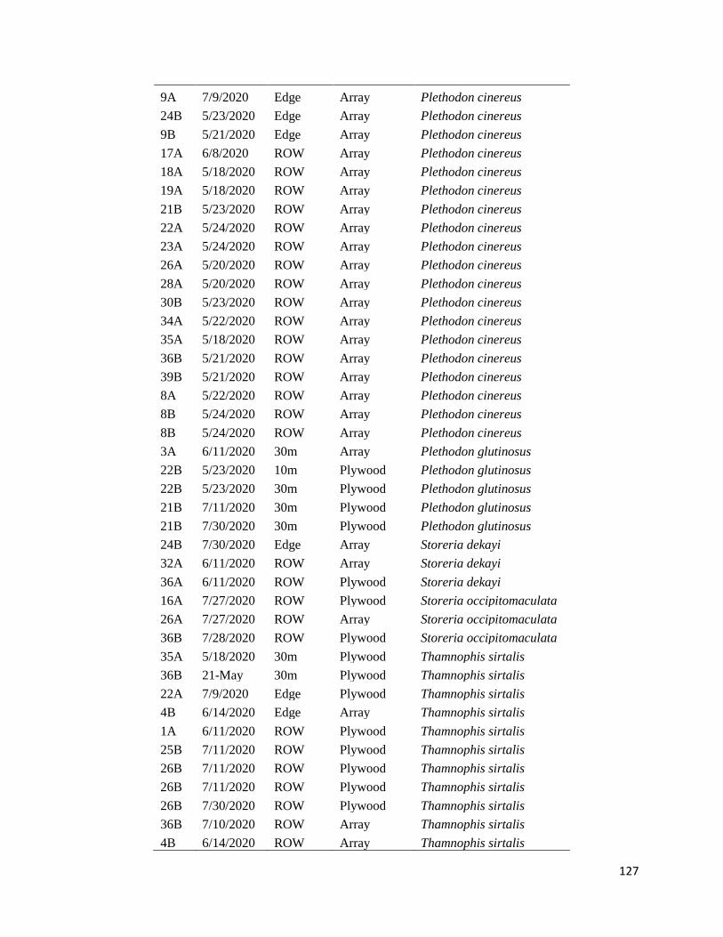
127
9A 7/9/2020 Edge Array Plethodon cinereus
24B 5/23/2020 Edge Array Plethodon cinereus
9B 5/21/2020 Edge Array Plethodon cinereus
17A 6/8/2020 ROW Array Plethodon cinereus
18A 5/18/2020 ROW Array Plethodon cinereus
19A 5/18/2020 ROW Array Plethodon cinereus
21B 5/23/2020 ROW Array Plethodon cinereus
22A 5/24/2020 ROW Array Plethodon cinereus
23A 5/24/2020 ROW Array Plethodon cinereus
26A 5/20/2020 ROW Array Plethodon cinereus
28A 5/20/2020 ROW Array Plethodon cinereus
30B 5/23/2020 ROW Array Plethodon cinereus
34A 5/22/2020 ROW Array Plethodon cinereus
35A 5/18/2020 ROW Array Plethodon cinereus
36B 5/21/2020 ROW Array Plethodon cinereus
39B 5/21/2020 ROW Array Plethodon cinereus
8A 5/22/2020 ROW Array Plethodon cinereus
8B 5/24/2020 ROW Array Plethodon cinereus
8B 5/24/2020 ROW Array Plethodon cinereus
3A 6/11/2020 30m Array Plethodon glutinosus
22B 5/23/2020 10m Plywood Plethodon glutinosus
22B 5/23/2020 30m Plywood Plethodon glutinosus
21B 7/11/2020 30m Plywood Plethodon glutinosus
21B 7/30/2020 30m Plywood Plethodon glutinosus
24B 7/30/2020 Edge Array Storeria dekayi
32A 6/11/2020 ROW Array Storeria dekayi
36A 6/11/2020 ROW Plywood Storeria dekayi
16A 7/27/2020 ROW Plywood Storeria occipitomaculata
26A 7/27/2020 ROW Array Storeria occipitomaculata
36B 7/28/2020 ROW Plywood Storeria occipitomaculata
35A 5/18/2020 30m Plywood Thamnophis sirtalis
36B 21-May 30m Plywood Thamnophis sirtalis
22A 7/9/2020 Edge Plywood Thamnophis sirtalis
4B 6/14/2020 Edge Array Thamnophis sirtalis
1A 6/11/2020 ROW Plywood Thamnophis sirtalis
25B 7/11/2020 ROW Plywood Thamnophis sirtalis
26B 7/11/2020 ROW Plywood Thamnophis sirtalis
26B 7/11/2020 ROW Plywood Thamnophis sirtalis
26B 7/30/2020 ROW Plywood Thamnophis sirtalis
36B 7/10/2020 ROW Array Thamnophis sirtalis
4B 6/14/2020 ROW Array Thamnophis sirtalis

128
4B 6/14/2020 ROW Array Thamnophis sirtalis
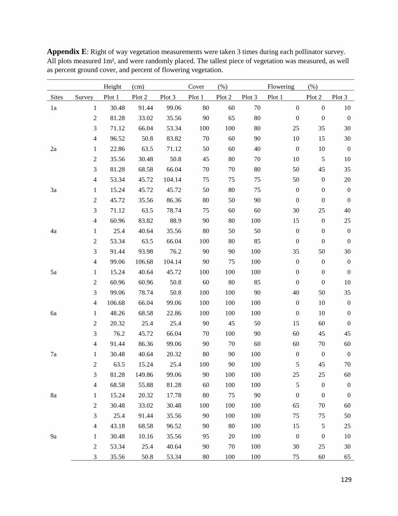
129
Appendix E: Right of way vegetation measurements were taken 3 times during each pollinator survey.
All plots measured 1m², and were randomly placed. The tallest piece of vegetation was measured, as well
as percent ground cover, and percent of flowering vegetation.
Height (cm) Cover (%) Flowering (%)
Sites Survey Plot 1 Plot 2 Plot 3 Plot 1 Plot 2 Plot 3 Plot 1 Plot 2 Plot 3
1a 1 30.48 91.44 99.06 80 60 70 0 0 10
2 81.28 33.02 35.56 90 65 80 0 0 0
3 71.12 66.04 53.34 100 100 80 25 35 30
4 96.52 50.8 83.82 70 60 90 10 15 30
2a 1 22.86 63.5 71.12 50 60 40 0 10 0
2 35.56 30.48 50.8 45 80 70 10 5 10
3 81.28 68.58 66.04 70 70 80 50 45 35
4 53.34 45.72 104.14 75 75 75 50 0 20
3a 1 15.24 45.72 45.72 50 80 75 0 0 0
2 45.72 35.56 86.36 80 50 90 0 0 0
3 71.12 63.5 78.74 75 60 60 30 25 40
4 60.96 83.82 88.9 90 80 100 15 0 25
4a 1 25.4 40.64 35.56 80 50 50 0 0 0
2 53.34 63.5 66.04 100 80 85 0 0 0
3 91.44 93.98 76.2 90 90 100 35 50 30
4 99.06 106.68 104.14 90 75 100 0 0 0
5a 1 15.24 40.64 45.72 100 100 100 0 0 0
2 60.96 60.96 50.8 60 80 85 0 0 10
3 99.06 78.74 50.8 100 100 90 40 50 35
4 106.68 66.04 99.06 100 100 100 0 10 0
6a 1 48.26 68.58 22.86 100 100 100 0 10 0
2 20.32 25.4 25.4 90 45 50 15 60 0
3 76.2 45.72 66.04 70 100 90 60 45 45
4 91.44 86.36 99.06 90 70 60 60 70 60
7a 1 30.48 40.64 20.32 80 90 100 0 0 0
2 63.5 15.24 25.4 100 90 100 5 45 70
3 81.28 149.86 99.06 90 100 100 25 25 60
4 68.58 55.88 81.28 60 100 100 5 0 0
8a 1 15.24 20.32 17.78 80 75 90 0 0 0
2 30.48 33.02 30.48 100 100 100 65 70 60
3 25.4 91.44 35.56 90 100 100 75 75 50
4 43.18 68.58 96.52 90 80 100 15 5 25
9a 1 30.48 10.16 35.56 95 20 100 0 0 10
2 53.34 25.4 40.64 90 70 100 30 25 30
3 35.56 50.8 53.34 80 100 100 75 60 65

130
4 17.78 50.8 45.72 90 100 80 0 10 0
10a 1 12.7 10.16 15.24 75 60 90 0 0 0
2 25.4 20.32 25.4 95 100 90 35 50 65
3 20.32 45.72 53.34 75 100 90 40 60 35
4 30.48 38.1 63.5 60 100 100 0 5 20
11a 1 38.1 15.24 33.02 80 95 100 0 0 0
2 81.28 45.72 81.28 90 100 100 10 5 0
3 76.2 25.4 86.36 100 100 100 30 40 30
4 91.44 99.06 71.12 100 100 100 25 20 10
12a 1 45.72 7.62 5.08 80 60 100 0 0 0
2 22.86 15.24 25.4 95 60 100 10 5 10
3 66.04 30.48 50.8 90 75 80 40 0 25
4 60.96 66.04 27.94 95 70 80 15 30 0
13a 1 12.7 15.24 12.7 90 100 70 0 0 0
2 15.24 22.86 35.56 100 100 100 10 10 0
3 7.62 0 25.4 30 0 80 15 0 30
4 66.04 20.32 15.24 100 80 80 10 25 30
14a 1 35.56 20.32 40.64 80 85 80 0 0 0
2 60.96 71.12 63.5 90 100 100 0 0 0
3 111.76 96.52 60.96 100 100 100 10 25 50
4 109.22 109.22 129.54 90 100 100 0 0 10
15a 1 35.56 15.24 27.94 80 75 90 0 0 0
2 20.32 33.02 35.56 75 100 100 5 0 0
3 68.58 88.9 99.06 90 100 100 60 60 50
4 81.28 99.06 45.72 70 100 90 15 15 10
16a 1 38.1 25.4 12.7 85 100 100 100 0 0
2 55.88 45.72 50.8 95 100 100 10 15 0
3 91.44 68.58 50.8 100 100 80 50 75 40
4 86.36 76.2 43.18 100 100 100 25 10 0
17a 1 30.48 45.72 15.24 50 90 80 0 0 0
2 40.64 50.8 60.96 50 45 75 0 10 0
3 91.44 71.12 76.2 100 60 80 15 20 30
4 99.06 50.8 48.26 100 40 100 10 10 30
18a 1 25.4 27.94 22.86 85 85 90 0 0 0
2 25.4 50.8 20.32 100 100 100 15 5 5
3 104.14 116.84 30.48 100 100 100 20 25 50
4 55.88 25.4 147.32 100 100 100 5 0 40
19a 1 35.56 58.42 55.88 100 85 80 0 0 0
2 81.28 50.8 76.2 60 50 75 0 0 0
3 86.36 116.84 114.3 100 100 100 0 20 50
4 114.3 93.98 40.64 90 90 100 20 35 10

131
20a 1 25.4 35.56 20.32 90 100 85 0 0 0
2 35.56 25.4 27.94 90 100 100 60 70 15
3 45.72 30.48 116.84 80 100 100 30 30 40
4 76.2 17.78 20.32 100 90 80 0 20 10
21a 1 25.4 35.56 20.32 100 100 50 5 0 0
2 55.88 40.64 30.48 85 75 80 0 0 5
3 86.36 25.4 99.06 50 50 80 10 20 25
4 109.22 93.98 50.8 80 100 100 20 20 0
22a 1 17.78 27.94 20.32 50 70 100 0 0 0
2 38.1 55.88 38.1 80 90 100 30 20 60
3 78.74 58.42 96.52 80 80 75 75 25 20
4 50.8 58.42 78.74 100 80 100 35 30 30
23a 1 25.4 40.64 12.7 100 70 100 0 0 0
2 33.02 68.58 50.8 100 100 100 50 0 65
3 119.38 83.82 35.56 100 100 90 30 40 60
4 106.68 116.84 38.1 100 100 90 0 0 0
24a 1 20.32 20.32 25.4 75 60 80 10 10 10
2 55.88 66.04 78.74 70 85 80 0 0 0
3 88.9 99.06 91.44 90 100 100 0 0 0
4 121.92 96.52 109.22 100 100 100 0 0 0
25a 1 30.48 20.32 50.8 100 50 100 0 0 0
2 45.72 38.1 40.64 80 100 70 0 0 5
3 63.5 0 71.12 80 0 100 15 0 20
4 96.52 17.78 88.9 80 15 70 0 0 15
26a 1 35.56 15.24 12.7 55 60 15 0 0 0
2 27.94 50.8 25.4 90 60 100 35 5 20
3 22.86 25.4 66.04 90 80 100 30 40 20
4 50.8 66.04 33.02 80 50 70 10 0 20
27a 1 5.08 10.16 5.08 20 65 10 0 0 0
2 17.78 25.4 15.24 55 100 65 30 30 10
3 38.1 60.96 30.48 60 85 90 20 50 20
4 20.32 33.02 22.86 25 25 60 0 10 0
28a 1 15.24 10.16 40.64 50 70 60 0 0 0
2 53.34 76.2 86.36 75 100 80 25 10 30
3 93.98 76.2 27.94 90 100 80 60 30 30
4 73.66 48.26 66.04 90 100 100 0 25 10
29a 1 0 15.24 15.24 0 10 50 0 0 0
2 30.48 38.1 25.4 10 20 10 0 0 0
3 0 53.34 20.32 0 60 10 0 0 0
4 48.26 0 27.94 80 0 50 0 0 5
30a 1 12.7 10.16 10.16 85 90 50 0 5 0

132
2 30.48 53.34 45.72 80 90 90 25 20 35
3 53.34 60.96 50.8 100 100 80 20 35 35
4 53.34 73.66 71.12 80 100 65 10 0 0
31a 1 66.04 152.4 124.46 70 100 100 0 0 0
2 35.56 53.34 38.1 100 100 80 30 0 0
3 71.12 88.9 93.98 90 100 100 10 0 0
4 104.14 91.44 78.74 100 100 100 10 5 0
32a 1 81.28 73.66 25.4 85 80 45 0 10 0
2 50.8 40.64 30.48 90 75 100 0 0 20
3 81.28 91.44 96.52 70 80 90 10 50 60
4 101.6 58.42 119.38 90 80 100 20 50 15
33a 1 12.7 10.16 20.32 30 80 50 0 0 10
2 48.26 55.88 43.18 90 100 100 0 0 0
3 30.48 35.56 40.64 50 60 75 20 15 30
4 104.14 38.1 33.02 90 80 75 40 40 30
34a 1 5.08 76.2 25.4 10 70 65 0 10 0
2 76.2 33.02 10.16 90 60 20 20 10 0
3 73.66 81.28 76.2 90 80 40 50 35 10
4 35.56 60.96 93.98 65 35 80 50 35 15
35a 1 129.54 106.68 116.84 100 90 100 0 0 0
2 60.96 101.6 86.36 100 100 100 0 0 0
3 106.68 91.44 66.04 100 100 80 0 30 20
4 109.22 124.46 134.62 80 80 100 0 0 0
36a 1 96.52 114.3 121.92 100 100 100 0 0 0
2 48.26 66.04 60.96 80 100 90 0 0 0
3 99.06 109.22 58.42 100 100 80 0 30 30
4 116.84 106.68 99.06 70 100 90 20 70 0
37a 1 60.96 38.1 76.2 45 55 70 0 0 0
2 40.64 53.34 50.8 45 50 80 0 0 0
3 81.28 58.42 68.58 75 60 100 10 25 25
4 86.36 93.98 66.04 50 90 80 5 50 25
38a 1 81.28 111.76 76.2 65 60 35 0 0 0
2 53.34 40.64 50.8 75 60 80 0 0 0
3 66.04 60.96 63.5 80 75 60 0 15 5
4 86.36 68.58 88.9 90 75 80 25 30 20
39a 1 40.64 35.56 45.72 90 100 100 20 0 10
2 78.74 86.36 25.4 100 100 90 0 0 30
3 81.28 71.12 63.5 95 100 80 25 0 0
4 93.98 109.22 86.36 100 100 100 5 25 35
40a 1 27.94 15.24 20.32 30 20 60 10 0 0
2 45.72 58.42 45.72 80 65 50 0 0 0

133
3 53.34 71.12 73.66 80 60 75 20 10 10
4 78.74 86.36 91.44 80 75 90 25 10 20
1b 1 66.04 78.74 30.48 80 90 100 0 10 0
2 66.04 55.88 50.8 90 80 100 0 0 0
3 81.28 63.5 99.06 100 100 100 75 60 75
4 99.06 106.68 114.3 100 100 100 50 20 75
2b 1 33.02 35.56 78.74 50 60 90 0 0 0
2 38.1 76.2 66.04 60 60 75 0 0 10
3 96.52 66.04 45.72 80 70 80 30 0 5
4 124.46 30.48 22.86 100 100 90 30 0 0
3b 1 25.4 20.32 30.48 80 80 70 0 0 0
2 60.96 25.4 25.4 85 70 80 0 0 0
3 20.32 66.04 35.56 75 80 70 0 0 20
4 50.8 25.4 48.26 80 90 100 5 0 15
4b 1 38.1 20.32 73.66 80 100 100 5 10 5
2 55.88 25.4 91.44 80 40 60 10 0 15
3 35.56 142.24 121.92 100 90 75 75 75 60
4 142.24 124.46 132.08 90 100 100 60 40 70
5b 1 43.18 50.8 10.16 100 100 100 0 0 15
2 35.56 48.26 40.64 70 80 60 0 0 0
3 83.82 33.02 93.98 100 60 90 60 10 25
4 76.2 50.8 83.82 80 100 90 10 70 20
6b 1 27.94 86.36 93.98 60 35 50 0 0 0
2 71.12 38.1 55.88 80 55 90 0 0 0
3 129.54 99.06 81.28 75 100 90 60 0 0
4 83.82 76.2 35.56 100 80 40 0 0 0
7b 1 43.18 25.4 40.64 100 100 100 0 0 0
2 40.64 53.34 60.96 90 60 75 0 0 10
3 86.36 91.44 78.74 90 100 100 10 35 40
4 137.16 147.32 127 75 100 80 5 0 15
8b 1 15.24 30.48 17.78 100 100 100 5 0 0
2 63.5 48.26 63.5 100 100 100 0 20 0
3 45.72 76.2 81.28 80 80 70 30 5 5
4 50.8 78.74 116.84 90 100 80 25 25 10
9b 1 10.16 25.4 58.42 100 100 100 0 0 0
2 55.88 63.5 53.34 70 50 60 0 0 0
3 86.36 43.18 66.04 100 100 100 0 0 5
4 73.66 81.28 81.28 90 90 90 0 0 0
10b 1 30.48 96.52 76.2 100 100 100 0 0 0
2 60.96 53.34 55.88 50 40 65 0 0 0
3 99.06 71.12 109.22 80 90 100 60 0 60

134
4 88.9 76.2 93.98 80 100 100 20 0 0
11b 1 81.28 25.4 15.24 100 100 100 0 0 0
2 55.88 66.04 66.04 80 75 50 0 0 0
3 96.52 106.68 91.44 80 90 100 0 30 0
4 101.6 93.98 96.52 100 100 90 0 0 0
12b 1 33.02 17.78 30.48 100 100 100 0 0 0
2 60.96 7.62 78.74 60 20 70 0 0 0
3 53.34 45.72 76.2 60 100 75 0 45 10
4 66.04 58.42 88.9 90 30 80 5 0 10
13b 1 15.24 20.32 20.32 80 90 85 0 0 0
2 50.8 27.94 25.4 80 70 70 0 0 0
3 60.96 45.72 68.58 40 50 75 0 0 10
4 55.88 25.4 60.96 60 70 50 0 0 0
14b 1 7.62 91.44 20.32 90 75 90 0 0 0
2 76.2 63.5 60.96 50 60 75 0 0 0
3 86.36 93.98 81.28 90 100 85 0 0 0
4 88.9 99.06 83.82 60 80 75 0 0 0
17b 1 25.4 142.24 121.92 100 100 100 10 0 0
2 50.8 76.2 104.14 80 90 80 0 0 0
3 81.28 144.78 177.8 80 100 100 0 40 50
4 187.96 170.18 129.54 100 100 100 90 90 50
18b 1 152.4 71.12 119.38 100 100 100 20 0 0
2 86.36 76.2 101.6 90 75 80 0 25 0
3 99.06 109.22 101.6 100 100 100 60 30 45
4 139.7 101.6 109.22 100 100 80 30 40 40
19b 1 5.08 73.66 35.56 100 80 100 0 0 10
2 25.4 38.1 60.96 30 75 90 0 30 0
3 101.6 99.06 45.72 60 100 75 0 0 0
4 96.52 86.36 88.9 100 100 100 15 0 0
20b 1 121.92 78.74 25.4 100 100 100 10 10 0
2 99.06 104.14 93.98 75 85 100 0 10 5
3 66.04 53.34 50.8 70 50 100 20 0 10
4 96.52 96.52 104.14 80 60 75 20 10 0
21b 1 5.08 91.44 53.34 100 80 100 0 20 0
2 35.56 50.8 55.88 60 50 80 0 0 50
3 96.52 104.14 76.2 75 90 80 0 50 0
4 101.6 109.22 96.52 100 80 100 0 20 0
22b 1 25.4 35.56 73.66 100 100 100 0 0 0
2 43.18 43.18 58.42 75 50 80 0 0 20
3 101.6 93.98 96.52 100 100 100 0 0 0
4 99.06 93.98 104.14 100 100 85 0 0 0

135
23b 1 35.56 15.24 60.96 100 100 100 0 0 0
2 78.74 50.8 60.96 85 40 75 0 0 60
3 81.28 50.8 40.64 80 75 40 0 0 0
4 33.02 53.34 20.32 40 75 50 0 0 0
24b 1 172.72 68.58 76.2 60 70 65 0 0 0
2 86.36 33.02 91.44 75 60 80 0 0 0
3 71.12 53.34 81.28 80 70 60 0 0 0
4 83.82 66.04 91.44 100 90 100 0 0 0
25b 1 15.24 22.86 17.78 100 80 85 0 0 0
2 58.42 50.8 45.72 60 80 80 0 5 15
3 58.42 66.04 76.2 80 100 90 0 0 20
4 93.98 96.52 116.84 70 100 100 0 0 25
26b 1 30.48 50.8 22.86 40 70 50 5 0 0
2 40.64 33.02 63.5 70 80 40 0 0 5
3 66.04 111.76 129.54 40 80 50 0 40 30
4 86.36 99.06 121.92 80 90 100 0 30 30
27b 1 99.06 20.32 30.48 85 70 55 5 0 0
2 50.8 58.42 66.04 55 40 50 0 0 0
3 73.66 76.2 91.44 90 100 90 20 0 0
4 81.28 93.98 106.68 90 75 100 0 0 0
28b 1 15.24 10.16 17.78 100 100 100 0 0 0
2 40.64 53.34 50.8 70 90 60 0 0 0
3 76.2 83.82 86.36 75 90 100 0 0 0
4 111.76 109.22 81.28 90 100 100 0 10 0
29b 1 10.16 15.24 15.24 50 80 100 0 0 0
2 45.72 60.96 45.72 80 90 60 0 0 0
3 96.52 96.52 88.9 90 100 100 0 0 0
4 106.68 88.9 66.04 100 100 80 0 10 10
30b 1 38.1 78.74 55.88 90 65 80 0 0 0
2 35.56 40.64 60.96 100 100 100 0 5 0
3 76.2 76.2 81.28 80 70 60 10 25 25
4 114.3 93.98 50.8 100 100 60 0 20 0
31b 1 15.24 17.78 30.48 80 70 100 0 15 0
2 63.5 50.8 12.7 85 80 35 0 25 0
3 53.34 50.8 22.86 85 100 65 25 40 50
4 38.1 88.9 93.98 80 90 100 0 5 0
32b 1 35.56 22.86 86.36 100 100 100 0 0 0
2 71.12 63.5 68.58 90 75 75 0 0 0
3 78.74 86.36 86.36 90 70 75 20 30 30
4 167.64 96.52 109.22 60 80 100 40 0 10
33b 1 144.78 83.82 30.48 100 100 100 0 0 0

136
2 20.32 48.26 60.96 90 60 35 40 0 10
3 43.18 78.74 66.04 100 80 80 40 15 25
4 104.14 109.22 66.04 80 70 90 0 30 15
34b 1 27.94 30.48 91.44 100 100 100 5 10 0
2 86.36 45.72 25.4 60 50 70 0 0 0
3 96.52 83.82 96.52 75 75 80 0 0 0
4 129.54 114.3 134.62 90 80 60 0 0 20
35b 1 30.48 45.72 20.32 100 100 100 0 0 0
2 66.04 76.2 76.2 50 80 60 0 0 0
3 93.98 99.06 101.6 90 80 65 25 10 0
4 78.74 86.36 86.36 70 85 60 0 20 0
36b 1 30.48 53.34 96.52 80 75 95 0 10 0
2 35.56 40.64 40.64 45 30 65 0 0 10
3 66.04 73.66 78.74 40 60 30 10 0 0
4 76.2 93.98 93.98 90 65 80 10 20 25
37b 1 78.74 60.96 25.4 80 70 100 0 0 10
2 33.02 45.72 50.8 60 50 75 0 0 10
3 104.14 86.36 30.48 90 50 50 35 0 10
4 68.58 33.02 58.42 80 60 50 10 10 5
38b 1 40.64 27.94 35.56 45 70 50 0 30 5
2 50.8 55.88 35.56 60 75 80 0 10 5
3 50.8 60.96 66.04 40 80 80 0 50 0
4 63.5 53.34 55.88 75 50 90 20 25 10
39b 1 66.04 25.4 78.74 100 100 100 0 0 0
2 91.44 50.8 58.42 65 45 70 20 0 0
3 116.84 71.12 83.82 100 80 90 30 40 0
4 63.5 96.52 73.66 80 95 100 10 0 20
40b 1 17.78 60.96 88.9 100 100 100 0 0 0
2 53.34 60.96 40.64 80 60 65 0 0 0
3 76.2 104.14 66.04 50 100 60 0 50 0
4 73.66 88.9 53.34 100 90 60 15 10 0
41b 1 25.4 15.24 27.94 100 100 100 0 0 0
2 60.96 71.12 60.96 80 100 60 0 0 0
3 114.3 104.14 109.22 100 100 100 10 0 0
4 96.52 93.98 86.36 100 100 80 5 10 0
42b 1 104.14 25.4 48.26 100 100 100 0 0 0
2 68.58 81.28 71.12 65 75 45 0 0 0
3 99.06 106.68 86.36 80 75 50 0 0 0
4 83.82 101.6 91.44 60 90 75 0 0 0

137
Appendix F: Forest structure measurements surrounding cover board sites. Canopy height was
measured using a laser rangefinder. Canopy cover was measured using a spherical densitometer, and is
the % of canopy covered. Tree count is the number of trees with a diameter at breast height (dbh) larger
than 15.24cm within 10m of the cover board. Tree DBH is the added dbh of tree count in cm. Stems were
counted within an 8m² plot around the cover boards.
stems stems stems stems
Site Loc
canopy
height
Canopy
Cover
Tree
count
Tree
dbh <2.54cm
2.54 -
7.62cm
7.62 -
15.24cm >15.24cm
1A ROW 0 0 0 0 0 0 0 0
1A Edge 4 69.84 3 48.26 0 4 4 2
1A 10m 5 89.86 5 78.74 0 1 6 0
1A 30m 5 89.86 5 78.74 0 1 6 0
2A ROW 0 0 0 0 0 0 0 0
2A Edge 12 66.72 6 129.54 1 5 6 0
2A 10m 10 85.96 4 68.58 8 5 6 1
2A 30m 10 85.96 4 68.58 8 5 6 1
3A ROW 0 0 0 0 0 0 0 0
3A Edge 4 62.82 4 96.52 2 0 0 0
3A 10m 8 87 5 111.76 0 0 2 0
3A 30m 8 87 5 111.76 0 0 2 0
4A ROW 0 0 0 0 0 0 0 0
4A Edge 4 60.22 7 144.78 7 2 3 2
4A 10m 8 85.7 7 121.92 19 0 3 0
4A 30m 8 85.7 7 121.92 19 0 3 0
5A ROW 0 0 0 0 0 0 0 0
5A Edge 4 82.58 4 109.22 1 0 0 7
5A 10m 7 88.56 4 142.24 3 3 0 0
5A 30m 7 88.56 4 142.24 3 3 0 0
6A ROW 0 0 0 0 0 0 0 0
6A Edge 5 30.84 2 33.02 0 0 1 0
6A 10m 8 90.64 6 198.12 3 1 0 0
6A 30m 8 90.64 6 198.12 3 1 0 0
7A ROW 0 0 0 0 0 0 0 0
7A Edge 10 66.2 4 147.32 4 1 2 0
7A 10m 8 92.2 8 307.34 4 1 0 1
7A 30m 8 92.2 8 307.34 4 1 0 1
8A ROW 0 0 0 0 0 0 0 0
8A Edge 10 53.46 3 88.9 9 1 1 0
8A 10m 10 87 10 281.94 0 4 1 0
8A 30m 10 87 10 281.94 0 4 1 0
9A ROW 0 0 0 0 0 0 0 0

138
9A Edge 11 86.22 6 195.58 0 1 0 1
9A 10m 14 85.7 13 353.06 11 2 0 4
9A 30m 14 85.7 13 353.06 11 2 0 4
10A ROW 0 0 0 0 0 0 0 0
10A Edge 10 90.38 7 185.42 7 1 3 0
10A 10m 4 93.24 0 0 11 14 2 0
10A 30m 4 93.24 0 0 11 14 2 0
11A ROW 0 0 0 0 0 0 0 0
11A Edge 10 74 5 124.46 0 0 0 0
11A 10m 10 90.12 6 198.12 1 4 0 1
11A 30m 10 90.12 6 198.12 1 4 0 1
12A ROW 0 0 0 0 0 0 0 0
12A Edge 5 72.18 2 55.88 0 0 0 1
12A 10m 6 78.94 4 88.9 2 0 0 1
12A 30m 6 78.94 4 88.9 2 0 0 1
13A ROW 0 0 0 0 0 0 0 0
13A Edge 3 68.54 1 50.8 0 3 1 0
13A 10m 2 90.12 3 55.88 2 0 1 0
13A 30m 2 90.12 3 55.88 2 0 1 0
14A ROW 0 0 0 0 0 0 0 0
14A Edge 10 70.1 3 96.52 14 0 0 0
14A 10m 8 85.44 6 226.06 1 2 0 2
14A 30m 8 85.44 6 226.06 1 2 0 2
15A ROW 0 0 0 0 0 0 0 0
15A Edge 4 32.92 2 93.98 6 0 0 0
15A 10m 8 69.06 4 157.48 3 0 0 0
15A 30m 8 69.06 4 157.48 3 0 0 0
16A ROW 0 0 0 0 0 0 0 0
16A Edge 3 87 7 175.26 0 1 2 1
16A 10m 10 76.08 10 200.66 7 1 2 0
16A 30m 10 76.08 10 200.66 7 1 2 0
17A ROW 0 0 0 0 0 0 0 0
17A Edge 8 26.68 1 15.24 0 6 0 0
17A 10m 6 92.98 3 109.22 0 3 0 0
17A 30m 6 92.98 3 109.22 0 3 0 0
18A ROW 0 0 0 0 0 0 0 0
18A Edge 0 0.16 0 0 0 0 0 0
18A 10m 5 56.84 6 129.54 2 1 0 0
18A 30m 5 56.84 6 129.54 2 1 0 0
19A ROW 0 0 0 0 0 0 0 0
19A Edge 2 92.2 9 185.42 7 0 0 2

139
19A 10m 5 89.08 20 538.48 2 3 0 2
19A 30m 5 89.08 20 538.48 2 3 0 2
20A ROW 0 0 0 0 0 0 0 0
20A Edge 6 78.94 1 17.78 2 1 1 0
20A 10m 8 90.38 6 203.2 4 2 0 1
20A 30m 8 90.38 6 203.2 4 2 0 1
21A ROW 0 0 0 0 0 0 0 0
21A Edge 2 63.08 7 200.66 10 1 0 0
21A 10m 4 89.6 18 502.92 6 0 2 0
21A 30m 4 89.6 18 502.92 6 0 2 0
22A ROW 0 0 0 0 0 0 0 0
22A Edge 5 87.78 0 0 8 2 2 0
22A 10m 5 90.64 0 0 0 6 3 0
22A 30m 5 90.64 0 0 0 6 3 0
23A ROW 0 0 0 0 0 0 0 0
23A Edge 5 48.52 4 124.46 7 1 0 0
23A 10m 6 88.56 6 127 4 0 0 1
23A 30m 6 88.56 6 127 4 0 0 1
24A ROW 0 0 0 0 0 0 0 0
24A Edge 10 63.6 4 147.32 3 0 2 0
24A 10m 13 82.06 9 271.78 2 1 0 4
24A 30m 13 82.06 9 271.78 2 1 0 4
25A ROW 0 0 0 0 0 0 0 0
25A Edge 6 48 4 180.34 5 1 1 1
25A 10m 6 90.38 4 109.22 0 0 2 0
25A 30m 6 90.38 4 109.22 0 0 2 0
26A ROW 0 0 0 0 0 0 0 0
26A Edge 0 18.1 2 50.8 5 1 1 1
26A 10m 8 16.28 2 43.18 0 0 0 0
26A 30m 8 16.28 2 43.18 0 0 0 0
27A ROW 0 0 0 0 0 0 0 0
27A Edge 13 20.7 2 99.06 0 0 0 0
27A 10m 13 32.4 3 139.7 4 0 0 1
27A 30m 13 32.4 3 139.7 4 0 0 1
28A ROW 0 0 0 0 0 0 0 0
28A Edge 6 49.56 7 213.36 0 1 0 1
28A 10m 10 76.08 10 292.1 2 0 0 2
28A 30m 10 76.08 10 292.1 2 0 0 2
29A ROW 0 0 0 0 0 0 0 0
29A Edge 10 78.16 7 248.92 4 1 0 1
29A 10m 10 90.64 11 330.2 3 4 0 0
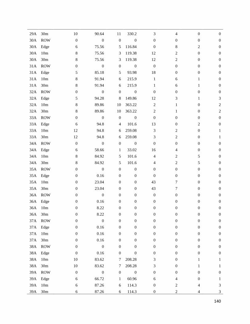
140
29A 30m 10 90.64 11 330.2 3 4 0 0
30A ROW 0 0 0 0 0 0 0 0
30A Edge 6 75.56 5 116.84 0 8 2 0
30A 10m 8 75.56 3 119.38 12 2 0 0
30A 30m 8 75.56 3 119.38 12 2 0 0
31A ROW 0 0 0 0 0 0 0 0
31A Edge 5 85.18 5 93.98 18 0 0 0
31A 10m 8 91.94 6 215.9 1 6 1 0
31A 30m 8 91.94 6 215.9 1 6 1 0
32A ROW 0 0 0 0 0 0 0 0
32A Edge 5 94.28 8 149.86 12 3 1 3
32A 10m 8 89.86 10 363.22 2 1 0 2
32A 30m 8 89.86 10 363.22 2 1 0 2
33A ROW 0 0 0 0 0 0 0 0
33A Edge 6 94.8 4 101.6 13 0 2 0
33A 10m 12 94.8 6 259.08 3 2 0 1
33A 30m 12 94.8 6 259.08 3 2 0 1
34A ROW 0 0 0 0 0 0 0 0
34A Edge 6 58.66 1 33.02 16 4 0 0
34A 10m 8 84.92 5 101.6 4 2 5 0
34A 30m 8 84.92 5 101.6 4 2 5 0
35A ROW 0 0 0 0 0 0 0 0
35A Edge 0 0.16 0 0 0 0 0 0
35A 10m 0 23.04 0 0 43 7 0 0
35A 30m 0 23.04 0 0 43 7 0 0
36A ROW 0 0 0 0 0 0 0 0
36A Edge 0 0.16 0 0 0 0 0 0
36A 10m 0 8.22 0 0 0 0 0 0
36A 30m 0 8.22 0 0 0 0 0 0
37A ROW 0 0 0 0 0 0 0 0
37A Edge 0 0.16 0 0 0 0 0 0
37A 10m 0 0.16 0 0 0 0 0 0
37A 30m 0 0.16 0 0 0 0 0 0
38A ROW 0 0 0 0 0 0 0 0
38A Edge 0 0.16 0 0 0 0 0 0
38A 10m 10 83.62 7 208.28 3 0 1 1
38A 30m 10 83.62 7 208.28 3 0 1 1
39A ROW 0 0 0 0 0 0 0 0
39A Edge 6 66.72 1 60.96 6 4 0 1
39A 10m 6 87.26 6 114.3 0 2 4 3
39A 30m 6 87.26 6 114.3 0 2 4 3

141
40A ROW 0 0 0 0 0 0 0 0
40A Edge 6 57.1 1 15.24 2 2 3 0
40A 10m 4 88.56 5 223.52 7 3 0 1
40A 30m 4 88.56 5 223.52 7 3 0 1
1B ROW 0 0 0 0 0 0 0 0
1B Edge 0 55.54 2 142.24 20 1 0 0
1B 10m 6 66.98 2 121.92 29 2 0 0
1B 30m 6 66.98 2 121.92 29 2 0 0
2B ROW 0 0 0 0 0 0 0 0
2B Edge 7 59.44 5 154.94 34 0 0 0
2B 10m 8 73.22 13 368.3 3 0 1 0
2B 30m 8 73.22 13 368.3 3 0 1 0
3B ROW 0 0 0 0 0 0 0 0
3B Edge 5 54.76 7 175.26 9 0 0 2
3B 10m 7 74.26 7 193.04 8 0 0 0
3B 30m 7 74.26 7 193.04 8 0 0 0
4B ROW 0 0 0 0 0 0 0 0
4B Edge 0 76.34 2 60.96 25 0 0 0
4B 10m 2 88.82 2 119.38 22 1 2 0
4B 30m 2 88.82 2 119.38 22 1 2 0
5B ROW 0 0 0 0 0 0 0 0
5B Edge 8 61.78 4 134.62 3 6 2 1
5B 10m 6 82.84 4 104.14 8 7 0 0
5B 30m 6 82.84 4 104.14 8 7 0 0
6B ROW 0 0 0 0 0 0 0 0
6B Edge 8 76.86 2 33.02 19 0 1 0
6B 10m 6 80.24 1 38.1 33 2 0 0
6B 30m 6 80.24 1 38.1 33 2 0 0
7B ROW 0 0 0 0 0 0 0 0
7B Edge 8 65.42 7 182.88 10 0 0 1
7B 10m 10 72.96 5 132.08 33 0 0 0
7B 30m 10 72.96 5 132.08 33 0 0 0
8B ROW 0 0 0 0 0 0 0 0
8B Edge 4 85.44 6 106.68 0 0 1 1
8B 10m 4 88.04 9 152.4 0 2 2 1
8B 30m 4 88.04 9 152.4 0 2 2 1
9B ROW 0 0 0 0 0 0 0 0
9B Edge 10 69.84 2 76.2 11 0 0 0
9B 10m 10 86.22 6 210.82 7 3 0 1
9B 30m 10 86.22 6 210.82 7 3 0 1
10B ROW 0 0 0 0 0 0 0 0

142
10B Edge 0 10.3 1 86.36 0 1 0 0
10B 10m 0 3.28 0 0 0 0 0 0
10B 30m 0 3.28 0 0 0 0 0 0
11B ROW 0 0 0 0 0 0 0 0
11B Edge 10 66.98 4 134.62 14 0 0 2
11B 10m 11 75.3 10 330.2 5 2 0 0
11B 30m 11 75.3 10 330.2 5 2 0 0
12B ROW 0 0 0 0 0 0 0 0
12B Edge 5 49.56 3 116.84 12 6 0 0
12B 10m 8 79.2 9 271.78 24 0 0 0
12B 30m 8 79.2 9 271.78 24 0 0 0
13B ROW 0 0 0 0 0 0 0 0
13B Edge 10 74 4 129.54 24 3 0 0
13B 10m 5 82.32 8 228.6 36 4 0 4
13B 30m 5 82.32 8 228.6 36 4 0 4
14B ROW 0 0 0 0 0 0 0 0
14B Edge 8 80.24 5 162.56 6 4 1 2
14B 10m 7 80.76 3 83.82 8 0 3 0
14B 30m 7 80.76 3 83.82 8 0 3 0
17B ROW 0 0 0 0 0 0 0 0
17B Edge 6 54.76 3 73.66 4 2 0 0
17B 10m 8 80.5 12 287.02 22 0 0 0
17B 30m 8 80.5 12 287.02 22 0 0 0
18B ROW 0 0 0 0 0 0 0 0
18B Edge 7 55.8 3 63.5 0 1 3 0
18B 10m 9 84.14 7 203.2 9 0 2 0
18B 30m 9 84.14 7 203.2 9 0 2 0
19B ROW 0 0 0 0 0 0 0 0
19B Edge 4 62.56 2 53.34 2 0 1 0
19B 10m 8 88.04 7 264.16 2 1 2 0
19B 30m 8 88.04 7 264.16 2 1 2 0
20B ROW 0 0 0 0 0 0 0 0
20B Edge 10 59.18 7 180.34 16 1 1 0
20B 10m 10 82.58 7 233.68 21 0 0 0
20B 30m 10 82.58 7 233.68 21 0 0 0
21B ROW 0 0 0 0 0 0 0 0
21B Edge 10 56.06 3 81.28 0 0 0 0
21B 10m 10 66.72 3 83.82 0 0 0 0
21B 30m 10 66.72 3 83.82 0 0 0 0
22B ROW 0 0 0 0 0 0 0 0
22B Edge 10 69.32 7 231.14 0 2 2 2

143
22B 10m 10 84.14 5 129.54 0 1 2 1
22B 30m 10 84.14 5 129.54 0 1 2 1
23B ROW 0 0 0 0 0 0 0 0
23B Edge 10 64.64 6 180.34 0 0 0 0
23B 10m 10 83.1 6 203.2 0 0 1 0
23B 30m 10 83.1 6 203.2 0 0 1 0
24B ROW 0 0 0 0 0 0 0 0
24B Edge 4 67.24 7 165.1 2 0 3 0
24B 10m 7 81.8 11 327.66 3 0 0 0
24B 30m 7 81.8 11 327.66 3 0 0 0
25B ROW 0 0 0 0 0 0 0 0
25B Edge 5 68.8 5 127 30 0 0 3
25B 10m 12 78.94 8 218.44 27 0 0 0
25B 30m 12 78.94 8 218.44 27 0 0 0
26B ROW 0 0 0 0 0 0 0 0
26B Edge 8 75.82 6 215.9 8 0 1 1
26B 10m 12 88.04 6 223.52 6 1 0 0
26B 30m 12 88.04 6 223.52 6 1 0 0
27B ROW 0 0 0 0 0 0 0 0
27B Edge 0 30.84 1 25.4 24 1 0 0
27B 10m 10 82.84 3 129.54 1 4 0 0
27B 30m 10 82.84 3 129.54 1 4 0 0
28B ROW 0 0 0 0 0 0 0 0
28B Edge 7 36.82 0 0 23 0 0 0
28B 10m 0 28.76 3 60.96 38 0 0 0
28B 30m 0 28.76 3 60.96 38 0 0 0
29B ROW 0 0 0 0 0 0 0 0
29B Edge 10 49.04 8 182.88 0 0 0 4
29B 10m 10 57.62 12 304.8 17 0 0 1
29B 30m 10 57.62 12 304.8 17 0 0 1
30B ROW 0 0 0 0 0 0 0 0
30B Edge 10 45.66 6 180.34 15 0 0 2
30B 10m 9 81.8 16 426.72 7 1 2 1
30B 30m 9 81.8 16 426.72 7 1 2 1
31B ROW 0 0 0 0 0 0 0 0
31B Edge 9 86.22 3 91.44 1 0 0 1
31B 10m 9 89.34 8 294.64 45 3 0 0
31B 30m 9 89.34 8 294.64 45 3 0 0
32B ROW 0 0 0 0 0 0 0 0
32B Edge 10 67.24 2 96.52 3 0 0 1
32B 10m 10 80.5 2 86.36 9 0 0 0

144
32B 30m 10 80.5 2 86.36 9 0 0 0
33B ROW 0 0 0 0 0 0 0 0
33B Edge 0 16.02 3 129.54 0 0 0 1
33B 10m 0 24.6 0 0 8 0 0 0
33B 30m 0 24.6 0 0 8 0 0 0
34B ROW 0 0 0 0 0 0 0 0
34B Edge 10 77.12 8 187.96 5 1 1 2
34B 10m 10 85.96 9 261.62 19 8 0 0
34B 30m 10 85.96 9 261.62 19 8 0 0
35B ROW 0 0 0 0 0 0 0 0
35B Edge 10 56.06 3 86.36 18 1 0 0
35B 10m 10 85.7 7 215.9 9 0 0 0
35B 30m 10 85.7 7 215.9 9 0 0 0
36B ROW 0 0 0 0 0 0 0 0
36B Edge 3 59.96 3 55.88 17 3 0 1
36B 10m 10 75.04 11 314.96 37 0 0 0
36B 30m 10 75.04 11 314.96 37 0 0 0
37B ROW 0 0 0 0 0 0 0 0
37B Edge 7 90.12 4 129.54 0 1 0 1
37B 10m 7 81.54 5 149.86 17 0 0 0
37B 30m 7 81.54 5 149.86 17 0 0 0
38B ROW 0 0 0 0 0 0 0 0
38B Edge 0 4.84 0 0 14 0 0 0
38B 10m 2 62.3 0 0 25 3 0 0
38B 30m 2 62.3 0 0 25 3 0 0
39B ROW 0 0 0 0 0 0 0 0
39B Edge 12 56.32 2 96.52 0 1 0 0
39B 10m 11 76.34 6 248.92 0 0 0 0
39B 30m 11 76.34 6 248.92 0 0 0 0
40B ROW 0 0 0 0 0 0 0 0
40B Edge 10 50.08 2 50.8 10 3 0 0
40B 10m 11 83.36 10 299.72 18 1 0 0
40B 30m 11 83.36 10 299.72 18 1 0 0
41B ROW 0 0 0 0 0 0 0 0
41B Edge 8 60.48 6 213.36 19 0 1 1
41B 10m 8 69.84 4 116.84 18 2 0 0
41B 30m 8 69.84 4 116.84 18 2 0 0
42B ROW 0 0 0 0 0 0 0 0
42B Edge 10 82.84 5 119.38 7 0 0 1
42B 10m 8 78.94 5 104.14 17 0 1 0
42B 30m 8 78.94 5 104.14 17 0 1 0

145
Appendix G: Seed mixes used to reclaim the ROW on the north-western pipeline within the Game
Lands 12 site. These mixes were planted in spring 2019. Study sites 4A – 30A were located on this ROW,
and the seed mix of each site is shown in appendix A. Each seed mix is numbered 1-16, and the
composition of species, percent by weight of each species, and seeding rate (lbs per acre) is shown.
Mix Common name Scientific name % / weight rate
1 annual oats - spring Avena sativa 61 50
annual ryegrass - fall loliummultiflorum 20
little bluestem schizachyrium scoparium 8
indian grass sorghastrum nutans 4
side oats grama Bouteloua curtipendula 2
switchgrass Panicum virgatum 2
black eyed susan Rudbeckia hirta 1
tall tickseed Coreopsis tripteris 1
sea oats uniola paniculata 2
2 virginia wildrye Elymus virginicus 32 15.75
partridge pea Chamaecrista fasciculata 19
little bluestem schizachyrium scoparium 25
indian grass sorghastrum nutans 13
switchgrass Panicum virgatum 6
brown eyed susan Rudbeckia triloba 2
lanceleaf coreopsis Coreopsis lanceolata 2
purple coneflower Echinacea purpurea 2
3 big bluestem - niagara Andropogon gerardii 38 8
eastern gama grass Tripsacum dactyloides 25
indian grass, PA ecotype sorghastrum nutans 19
marsh blazing star Liatris spicata 5
queen annes lace Daucus carota 2
maximillian sunflower Helianthus maximilianii 2
smooth blue aster Aster laevis 2
perennial gaillardia Gaillardia aristata 2
cup plant silphium perfoliatum 2
golden alexanders Zizia aurea 2
ohio spiderwort Tradescantia ohiensus 2
wild bergamot Monarda fistulosa 1
4 little bluestem, PA ecotype schizachyrium scoparium 22 8
broomsedge Androgen virginicus 22
indiangrass sorghastrum nutans 18
riverbank wildrye Elymus riparius 15
purpletop Tridens flavus 4
tall white beardtongue, PA ecotype Penstemon digitalis 2

146
maximillian sunflower Helianthus maximilianii 7
swamp milkweed, PA ecotype Asclepias incarnata 1
common milkweed, PA ecotype Asclepias syriaca 1
smooth blue aster Aster laevis 1
new england aster Aster novae-angliae 1
white avens, PA ecotype Geum canadense 1
blue false indigo Baptista australis 1
wild senna Senna hebecarpa 1
narrow leafed blue-eyed grass Sisyrinchium angustifolium 1
ohio spiderwort, PA ecotype Tradescantia ohiensus 1
golden alexanders Zizia aurea 1
wild bergamot, PA ecotype Monarda fistulosa 0.5
early goldenrod, PA ecotype Solidago juncea 0.2
gray goldenrod, PA ecotype Solidago nemoralis 0.2
5 side oats grama Bouteloua curtipendula 33 8
little bluestem, PA ecotype schizachyrium scoparium 33
broomsedge Androgen virginicus 17
purple coneflower Echinacea purpurea 4
maximillian sunflower Helianthus maximilianii 3
partridge pea Chamaecrista fasciculata 2
lance leafed coreopsis Coreopsis lanceolata 2
black eyed susan Rudbeckia hirta 2
gray headed coneflower Ratibida pinnata 1
wild senna Senna hebecarpa 1
6 birds-foot trefoil Lotus corniculatus 18 158
alsike clover Trifolium hybridum 10
white clover, Dutch Trifolium repens 6
white clover, ladino Trifolium repens 13
medium red clover Trifolium pratense 16
dwarf essex rape Brassica napus 6
oats or wheat 23
7 little bluestem schizachyrium scoparium 40 8
indian grass sorghastrum nutans 23
wildrye Elymus spp. 17
maximillian sunflower Helianthus maximilianii 2
purple coneflower Echinacea purpurea 2
black eyed susan Rudbeckia hirta 2
lance leafed coreopsis Coreopsis lanceolata 2
partridge pea Chamaecrista fasciculata 2
cup plant silphium perfoliatum 2
smooth blue aster Aster laevis 1

147
showy trick trefoil Desmodium canadense 1
grey headed coneflower Ratibida pinnata 1
hairy beardtongue Penstemon hirsutus 1
rough gayfeather Liatris aspera 1
wild senna Senna hebecarpa 1
8 side oats grama Bouteloua curtipendula 33 8
little bluestem schizachyrium scoparium 33
broomsedge Androgen virginicus 17
purple coneflower Echinacea purpurea 4
maximillian sunflower Helianthus maximilianii 3
partridge pea Chamaecrista fasciculata 2
lance leafed coreopsis Coreopsis lanceolata 2
black eyed susan Rudbeckia hirta 2
grey headed coneflower Ratibida pinnata 1
wild senna Senna hebecarpa 1
9 2 + 6
10 3 + 6
11 4 + 6
12 5 + 6
13 6 + 8
14 wetland
15 virginia wildrye Elymus virginicus 22 20
big bluestem - niagara Andropogon gerardii 16
indiangrass sorghastrum nutans 15
switchgrass Panicum virgatum 14
partridge pea Chamaecrista fasciculata 6
autumn bentgrass Agrostis perennans 6
blue vervain Verbena hastata 4
oxeye sunflower Heliopsis helianthoides 3
black eyed susan Rudbeckia hirta 3
boneset Eupatorium perfoliatum 2
giant ironweed Vernonia angustifolia 2
soft rush Juncus effusus 2
swamp sunflower Helianthus angustifolius 1
blue false indigo Baptisiaaustralis 1
joe pye weed Eupatorium fistulosum 1
great blue lobelia Lobelia siphilitca 1
wild bergamot Monarda fistulosa 1
16 Alsike clover Trifolium hybridum 7 72
white dutch clover Trifolium repens 7

148
ladino clover Trifolium repens 7
medium red clover Trifolium pratense 7
aspen seedlings Populus tremuloides 0
dwarf essex rape Brassica napus 1
oats or wheat 70

149
Appendix H: Butterfly species present in Bradford and Lycoming counties of Pennsylvania from
Butterflies of Pennsylvania (Monroe and Wright 2017). Visually similar species which are difficult to
distinguish from photographs were grouped together and counted as one species when encountered (ID
Group).
Species scientific name
ID
group
Pipevine swallowtail Battus philenor 1
black swallowtail Papilio polyxenes 2
Giant Swallowtail Papilio cresphontes 3
Eastern Tiger Swallowtail Papilio glaucus 4
Canadian Tiger
Swallowtail Papilio canadensis 4
SpiceBush Swallowtail Papilio troilus 5
West Virginia White Pieris virginiensis 6
Cabbage White Pieris rapae 7
Clouded Sulphur Colias philodice 8
Orange Sulphur Colias eurytheme 8
Little Yellow Pyrisitia lisa 8
Harvester Feniseca tarquinius 9
American Copper Lycaena phlaeas 10
Bronze Copper Lycaena hyllus 10
Bog Copper Lycaena epixanthe 11
Coral Hairstreak Satyrium titus 12
Acadian Hairstreak Satyrium acadica 12
Edwards Hairstreak Satyrium edwardsii 12
Banded Hairstreak Satyrium calanus 12
Hickory Hairstreak Satyrium caryaevorus 12
Striped Hairstreak Satyrium liparops 12
Oak Hairstreak Satyrium favonius 12
Brown Elfin Callophrys augustinus 13
Frosted Elfin Callophrys irus 13
Eastern Pine Elfin Callophrys niphon 13
Gray Hairstreak Strymon melinus 14
Eastern Tailed Blue Cupido comyntas 15
Northern Spring Azure Celastrina lucia 16
Summer Azure Celastrina neglecta 17
Cherry Gall Azure Celastrina serotina 17
American Snout Libytheana carinenta 18
Monarch Danaus plexippus 19
Variegated Fritillary Euptoieta claudia 20
Great Spangled Fritillary Speyeria cybele 21

150
Aphrodite Fritillary Speyeria aphrodite 21
Atlantis Fritillary Speyeria atlantis 21
Regal Fritillary Speyeria idalia 21
Silver-bordered fritillary Boloria selene 21
Meadow fritillary Boloria bellona 21
Harris' checkerspot Chlosyne harrisii 22
Baltimore checkerspot Euphydryas phaeton 22
Pearl Crescent Phyciodes tharos 23
Northern Crescent Phyciodes cocyta 23
Common Buckeye Junonia coenia 24
Question Mark Polygonia interrogationis 25
Eastern Comma Polygonia comma 25
Green Comma Polygonia faunus 25
Gray Comma Polygonia progne 25
Compton Tortoiseshell Nymphalis l-album 25
Morning Cloak Nymphalis antiopa 26
Milbert's Tortoiseshell Aglais milberti 27
American Lady Vanessa virginiensis 28
Painted Lady Vanessa cardui 29
Red Admiral Vanessa atalanta 30
White Admiral Limenitis arthemis arthemis 31
Red-spotted Purple Limenitis arthemis astyanax 32
Viceroy Limenitis archippus 33
Hackberry Emperor Asterocampa celtis 34
Tawny Emperor Asterocampa clyton 35
Northern Pearly-Eye Lethe anthedon 36
Eyed Brown Lethe eurydice 36
Appalachian Brown Leethe appalachia 36
Little Wood Satyr Megisto cymela 37
Common Ringlet Coenonympha tullia 38
Common Wood Nymph Cercyonia pegala 39
Silver-spotted Skipper Epargyreus clarus 40
Hoary Edge Achalarus lyciades 40
Northern Cloudywing Thorybes pylades 41
Dreamy Duskywing Erynnis icelus 41
Sleepy Duskywing Erynnis brizo 41
Juvenal's Duskywing Erynnis juvenalis 41
Mottled Duskywing Erynnis martialis 41
Wild Indigo Duskywing Erynnis baptisiae 41
Common Sootywing Pholisora catullus 41

151
common checkered-
skipper Pyrgus communis 41
Least Skipper Ancyloxypha numitor 42
European Skipper Thymelicus lineola 42
Leonard's Skipper Hesperia leonardus 42
Cobweb Skipper Hesperia metea 42
Indian Skipper Hesperia sassacus 42
Peck's Skipper Polites peckius 42
Tawny-edged Skipper Polites themistocles 42
Crossline Skipper Polites origenes 42
Long Dash Polites mystic 42
Little Glassywing Pompeius verna 42
Northern Broken-Dash Wallengrenia egeremet 42
Delaware Skipper Anatrytine logan 42
Zabulon Skipper Poanes zabulon 42
Hobomok Skipper Poanes hobomok 42
Dion Skipper Euphyes dion 42
Two-Spotted Skipper Euphyes bimacula 42
Dun Skippper Euphyes vestris 42
Common Roadside-
Skipper Amblyscirtes vialis 42

152
Appendix I: Pollinator encounters during each survey. Data are broken up by site, survey, and year. Abundance was not recorded during 2019,
but was in 2020. ETB is an abbreviation of Eastern tailed blue. Bees were not separated by species or group.
2019 2020
1A Survey 1 Species 1A Survey 1 Species
Survey 2 Species Survey 2 Species
Survey 3 Species Survey 3 Species
Monarch, skipper 2 sulphur, 3 ETB, 2 wood nymph, 1 fritillary, 1 yellow swallowtail
Survey 4 Species Survey 4 Species
sulphur , duskywing, bee
5 wood nymph, 2 fritillary, 1 sulphur, 2 brown skipper, 3 least skipper 1
ETB
2A Survey 1 Species 2A Survey 1 Species
Survey 2 Species Survey 2 Species
skipper, eastern tailed blue, bee
Survey 3 Species Survey 3 Species
3 fritillary, 2 sulphur, 6 bee, 1 wood nymph, 2 least skipper
Survey 4 Species Survey 4 Species
swallowtail, duskywing, eastern tailed blue
2 sulphur, 5 bee, 1 honey bee, 3 least skipper, 5 bee, 1 ETB, 1
cloudywing
3A Survey 1 Species 3A Survey 1 Species
Survey 2 Species Survey 2 Species
Survey 3 Species Survey 3 Species
swallowtail, skipper, bee 2 fritillary, 1 sulphur, 2 least skipper, 2 bee
Survey 4 Species Survey 4 Species
monarch, sulphur, eastern tailed blue 2 brown skipper, 3 bee, 1 wood nymph
153
4A Survey 1 Species 4A Survey 1 Species
Survey 2 Species Survey 2 Species
1 sulphur sp.
Survey 3 Species Survey 3 Species
american lady, monarch, skipper 3 least skipper, 3 bee, 1 honey bee, 1 sulphur
Survey 4 Species Survey 4 Species
skipper 1 wood nymph, 2 sulphur
5A Survey 1 Species 5A Survey 1 Species
Survey 2 Species Survey 2 Species
swallowtail 1 cabbage white
Survey 3 Species Survey 3 Species
skipper 4 least skipper, 9 bees, 1 ETB, 1 honeybee
Survey 4 Species Survey 4 Species
cabbage white, sulphur, crescent, eastern tailed
blue 1 least skipper, 2 bee
6A Survey 1 Species 6A Survey 1 Species
Survey 2 Species Survey 2 Species
1 sulphur, 4 blue damselflies, 5 bumblebee, 1 honey bee
Survey 3 Species Survey 3 Species
skipper
1 cabbage white, 1 wood nymph, 8 bee, 2 cloudywing, 5 ETB, 1
fritillary
Survey 4 Species Survey 4 Species
cabbage white 7 ETB, 8 fritillary, 2 cabbage white, 2 bee, 6 honey bee, 1 sulphur
7A Survey 1 Species 7A Survey 1 Species
american lady
Survey 2 Species Survey 2 Species
bee 2 sulphurs, 8 bees, 3 honey bees

154
Survey 3 Species Survey 3 Species
skipper, cabbage white 11 least skipper, 2 duskywing sp., 1 bee, 2 ETB, 2 fritillary
Survey 4 Species Survey 4 Species
skipper, cabbage white 1 bee, 1 wood nymph, 1 brown skipper
8A Survey 1 Species 8A Survey 1 Species
Survey 2 Species Survey 2 Species
1 cabbage white, 6 bees, 1 cloudywing, 1 yellow swallowtail
Survey 3 Species Survey 3 Species
1 cabbage white, 7 Eastern Tailed Blue, 7 Least Skipper, 3 bee, 1
sulphur
Survey 4 Species Survey 4 Species
cabbage white 2 brown skipper, 2 ETB, 1 sulphur
9A Survey 1 Species 9A Survey 1 Species
duskywing 2 bumblebees
Survey 2 Species Survey 2 Species
1 yellow swallowtail, 1 cabbage white, 1 bee, 1 common ringlet
Survey 3 Species Survey 3 Species
red admiral 1 yellow swallowtail, 2 bee, 5 skippers, 2 Eastern Tailed Blue
Survey 4 Species Survey 4 Species
sulphur, cabbage white, skipper 1 sulphur
10A Survey 1 Species 10A Survey 1 Species
skipper 1 wasp
Survey 2 Species Survey 2 Species
2 eastern blue, 2 bumble bee, 1 yellow swallowtail, 1 sulphur, 1
skipper, 4 honey bee, 5 bee
Survey 3 Species Survey 3 Species
cabbage white, sulphur 2 sulphur, 4 ETB, 1 skipper, 2 bee, 1 fritillary
Survey 4 Species Survey 4 Species
cabbage white 1 brown skipper, 5 sulphur, 1 cabbage white, 1 ETB, 2 bee

155
11A Survey 1 Species 11A Survey 1 Species
Survey 2 Species Survey 2 Species
bee 1 yellow swallowtail
Survey 3 Species Survey 3 Species
cabbage white, fritillary 1 ETB, 8 honeybee, 7 bee, 1 least skipper
Survey 4 Species Survey 4 Species
2 ETB, 2 bee, 1 sulphur
12A Survey 1 Species 12A Survey 1 Species
swallowtail
Survey 2 Species Survey 2 Species
1 bumblebee
Survey 3 Species Survey 3 Species
3 honey bee, 2 med orange fritillary, 1 bee, 3 ETB, 2 sulphur
Survey 4 Species Survey 4 Species
monarch 2 sulphur, 2 ETB, partially reseeded
13A Survey 1 Species 13A Survey 1 Species
1 bumblebee
Survey 2 Species Survey 2 Species
2 bee
Survey 3 Species Survey 3 Species
fritillary, cabbage white, sulphur
Survey 4 Species Survey 4 Species
cabbage white, swallowtail, sulphur 2 brown skipper, 8 bee, 1 cabbage white, 1 sulphur, 1 ETB
14A Survey 1 Species 14A Survey 1 Species
Survey 2 Species Survey 2 Species
2 sulphur, 1 Red Admiral
Survey 3 Species Survey 3 Species

156
2 bee, 1 sulphur, 1 ETB
Survey 4 Species Survey 4 Species
cabbage white, sulphur, swallowtail
15A Survey 1 Species 15A Survey 1 Species
red admiral, bee
Survey 2 Species Survey 2 Species
1 sulphur
Survey 3 Species Survey 3 Species
american lady 12 bee, 3 least skipper, 3 sulphur, 4 fritillary, 1 honey bee, 1 ETB,
Survey 4 Species Survey 4 Species
american lady, skipper, cabbage white, eastern
tailed blue , sulhpur, bee 6 ETB, 3 sulphur, 1 bee, 1 lg fritillary
16A Survey 1 Species 16A Survey 1 Species
1 sulphur sp.
Survey 2 Species Survey 2 Species
2 bumble bee
Survey 3 Species Survey 3 Species
cabbage white 10 bee, 4 fritillary, 4 least skipper, 3 honey bee, 1 ETB, 1 sulphur
Survey 4 Species Survey 4 Species
cabbage white, sulphur 3 sulphur, 5 bee, 1 ETB, 2 brown skipper, 1 cabbage white
17A Survey 1 Species 17A Survey 1 Species
Survey 2 Species Survey 2 Species
bee 1 bumblebee, 1 swallowtail
Survey 3 Species Survey 3 Species
4 fritillary, 1 sulphur, 2 ETB, 3 bee
Survey 4 Species Survey 4 Species
1 yellow swallowtail, 4 sulphur, 4 fritillary, 7 brown skipper, 2 ETB, 6
bee, 1 sweat bee, 3 least skipper
18A Survey 1 Species 18A Survey 1 Species

157
Survey 2 Species Survey 2 Species
1 sulphur, 1 least skipper, 1 yellow swallowtail
Survey 3 Species Survey 3 Species
cabbage white, skipper, bee 3 ETB, 4 bee, 2 fritillary, 2 least skipper
Survey 4 Species Survey 4 Species
cabbage white, skipper, bee
1 sulphur, 1 sweat bee, 1 monarch, 7 fritillary, 17 bee, 2 brown skipper,
thistle
19A Survey 1 Species 19A Survey 1 Species
Survey 2 Species Survey 2 Species
1 bumblebee, 1 cabbage white
Survey 3 Species Survey 3 Species
sulphur, fritillary 1 fritillary, 12 bees, 1 honey bee
Survey 4 Species Survey 4 Species
cabbage white 2 fritillary, 2 bee, 6 ETB, 1 sulphur
20A Survey 1 Species 20A Survey 1 Species
1 sulphur sp., 1 bumblebee
Survey 2 Species Survey 2 Species
eastern tailed blue, duskywing 1 sulphur, 15 bee, 6 honey bee, 1 american lady
Survey 3 Species Survey 3 Species
cabbage white, skipper 5 bee, 2 fritillary, 2 least skipper, 2 sulphur, 2 ETB, 4 honeybee
Survey 4 Species Survey 4 Species
cabbage white, sulphur, bee 1 ETB, 2 sulphur, 3 honey bee, 1 brown skipper, 2 fritillary, 1 bee
21A Survey 1 Species 21A Survey 1 Species
Survey 2 Species Survey 2 Species
2 sulphurs, 1 honey bee
Survey 3 Species Survey 3 Species

158
cabbage white 2 wood nymph, 3 brown skipper
Survey 4 Species Survey 4 Species
cabbage white, sulphur, fritillary, bee 4 ETB, 1 sulphur, 2 bee, 3 least skipper
22A Survey 1 Species 22A Survey 1 Species
1 yellow sulphur
Survey 2 Species Survey 2 Species
checkerspot, cabbage white, bee 2 bumblebee, 2 honey bee
Survey 3 Species Survey 3 Species
2 honeybee, 8 bees, 6 ETB, 6 fritillary, 3 skipper
Survey 4 Species Survey 4 Species
American lady, cabbage white, bee 2 fritillary, 3 bee, 2 sulphur, 1 ETB
23A Survey 1 Species 23A Survey 1 Species
1 eastern tailed blue, 1 yellow sulphur
Survey 2 Species Survey 2 Species
2 small bumblebees, 10 bee, 1 ETB
Survey 3 Species Survey 3 Species
cabbage white, skipper 2 fritillary, 2 ETB, 7 bee, 2 skipper
Survey 4 Species Survey 4 Species
cabbage white, sulphur 1 sulphur, 1 brown skipper
24A Survey 1 Species 24A Survey 1 Species
1 bumblebee
Survey 2 Species Survey 2 Species
Survey 3 Species Survey 3 Species
Survey 4 Species Survey 4 Species
american lady 1 ETB
25A Survey 1 Species 25A Survey 1 Species
2 eastern tailed blue, 1 cabbage white, 2 bumblebee

159
Survey 2 Species Survey 2 Species
1 yellow swallowtail
Survey 3 Species Survey 3 Species
cabbage white 1 brown skipper, 1 fritillary
Survey 4 Species Survey 4 Species
cabbage white, american lady, swallowtail 4 brown skipper, 1 fritillary, 2 ETB, 2 bee
26A Survey 1 Species 26A Survey 1 Species
1 sulphur sp.
Survey 2 Species Survey 2 Species
common ringlet, sulphur, american lady,
cabbage white 1 sulphur sp., 3 bee
Survey 3 Species Survey 3 Species
8 bee, 3 honeybee, 2 least skipper, 2 ETB
Survey 4 Species Survey 4 Species
cabbage white 3 ETB, 6 brown skipper
27A Survey 1 Species 27A Survey 1 Species
Survey 2 Species Survey 2 Species
red spotted purple 1 cabbage white, 16 bee
Survey 3 Species Survey 3 Species
cabbage white, fritillary
3 sulphur, 1 wood nymph, 3 bee, 1 honey bee, 2 least skipper, 2 ETB, 1
med orange fritillary
Survey 4 Species Survey 4 Species
cabbage white, sulphur 2 sulphur, 4 ETB, 6 bee
28A Survey 1 Species 28A Survey 1 Species
Survey 2 Species Survey 2 Species
2 sulphur, 6 bumblebee, 1 honey bee, 1 ETB
Survey 3 Species Survey 3 Species
cabbage white, sulphur 4 fritillary, 1 sulphur, 2 least skipper, 1 bee
160
Survey 4 Species Survey 4 Species
cabbage white, sulphur 5 sulphur, 1 ETB, 1 cabbage white
29A Survey 1 Species 29A Survey 1 Species
Survey 2 Species Survey 2 Species
Survey 3 Species Survey 3 Species
Survey 4 Species Survey 4 Species
sulphur 1 cabbage white, 1 american lady, 1 ETB
30A Survey 1 Species 30A Survey 1 Species
Survey 2 Species Survey 2 Species
red admiral, bee 1 sulphur, 2 bumblebee, 1 honeybee
Survey 3 Species Survey 3 Species
cabbage white 3 bee, 2 ETB, 1 fritillary
Survey 4 Species Survey 4 Species
cabbage white, sulphur, bee 1 fritillary, 2 bee
31A Survey 1 Species 31A Survey 1 Species
sulphur, american lady
Survey 2 Species Survey 2 Species
2 honey bee, 1 eastern tailed blue
Survey 3 Species Survey 3 Species
fritillary, skipper 2 sulphur, 2 ETB
Survey 4 Species Survey 4 Species
monarch, sulphur, bee 1 sulphur, 1 sweat bee
32A Survey 1 Species 32A Survey 1 Species
black swallowtail
Survey 2 Species Survey 2 Species

161
bee
Survey 3 Species Survey 3 Species
eastern tailed blue 1 bee, 3 fritillary, 2 honey bee, 1 moth
Survey 4 Species Survey 4 Species
sulphur, swallowtail, skipper, eastern tailed
blue, cabbage white, bee 2 ETB, 2 sulphur, 4 bee, 3 skipper
33A Survey 1 Species 33A Survey 1 Species
bee
Survey 2 Species Survey 2 Species
Survey 3 Species Survey 3 Species
bee 2 least skipper, 1 honey bee
Survey 4 Species Survey 4 Species
eastern tailed blue, skipper , sulhpur, fritillary,
bee 2 sulphur, 2 fritillary, 5 bee, 7 honey bee
34A Survey 1 Species 34A Survey 1 Species
bee
Survey 2 Species Survey 2 Species
Survey 3 Species Survey 3 Species
3 sulphur, 2 ETB, 5 fritillary, 2 checkerspot
Survey 4 Species Survey 4 Species
cabbage white, sulphur, azure sp., swallowtail,
fritillary, bee
3 brown skipper, 11 bee, 5 fritillary, 1 sulphur, 1 least skipper, 1 wasp,
1 wood nymph
35A Survey 1 Species 35A Survey 1 Species
american lady, bee
Survey 2 Species Survey 2 Species
Survey 3 Species Survey 3 Species
swallowtail, bee 1 flower fly, 1 honey bee

162
Survey 4 Species Survey 4 Species
bee
36A Survey 1 Species 36A Survey 1 Species
azure spp., bee
Survey 2 Species Survey 2 Species
red spotted purple, skipper, bee 1 cabbage white, 1 sulphur
Survey 3 Species Survey 3 Species
painted lady, skipper
1 yellow swallowtail, 2 sulphur, 1 wood nymph, 1 sweat bee, 1 brown
skipper
Survey 4 Species Survey 4 Species
american lady, sulphur, black swallowtail,
eastern tailed blue 1 monarch, 5 bee, 2 least skipper
37A Survey 1 Species 37A Survey 1 Species
cabbage white, bee
Survey 2 Species Survey 2 Species
monarch, american lady, bee
Survey 3 Species Survey 3 Species
skipper, cabbage white, sulphur, fritillary 5 bees, 1 least skipper
Survey 4 Species Survey 4 Species
sootywing, sulphur, azure spp. 1 bee, 1 wood nymph, 1 monarch
38A Survey 1 Species 38A Survey 1 Species
bee
Survey 2 Species Survey 2 Species
swallowtail, skipper , painted lady, american
lady, red spotted purple, bee
Survey 3 Species Survey 3 Species
swallowtail, eastern tailed blue, skipper, bee 1 sulphur, 4 ETB, 1 bee, 1 fritillary
Survey 4 Species Survey 4 Species
monarch, eastern tailed blue, sulphur, bee 1 ETB, 3 bee
39A Survey 1 Species 39A Survey 1 Species

163
cabbage white, bee 1 cabbage white, 1 flower fly
Survey 2 Species Survey 2 Species
1 honey bee, 1 cabbage white
Survey 3 Species Survey 3 Species
3 brown skipper, 1 sulphur
Survey 4 Species Survey 4 Species
cabbage white, sulphur, skipper , swallowtail,
monarch 2 monarch, 2 fritillary, 1 bee, 3 brown skipper, 1 sulphur
40A Survey 1 Species 40A Survey 1 Species
1 red admiral
Survey 2 Species Survey 2 Species
Survey 3 Species Survey 3 Species
cabbage white, sulphur 2 least skipper, 1 fritillary
Survey 4 Species Survey 4 Species
cabbage white, sulphur, azure spp. 3 least skipper, 4 bee, 1 wood nymph, 1 yellow swallowtail
1B Survey 1 Species 1B Survey 1 Species
Survey 2 Species Survey 2 Species
Survey 3 Species Survey 3 Species
monarch, skipper, bee
1 wood nymph, 18 bee, 2 yellow swallowtail, 1 ETB, 4 honey bee, 1
brown skipper
Survey 4 Species Survey 4 Species
monarch, swallowtail, duskywing, sulphur, bee
32 bee, 2 checkerspot, 3 black swallowtail, 2 sulphur, 3 honey bee, 3
monarch, 1 wood nymph, 2 yellow swallowtail, 1 cloudywing, invasive
pea plant thing
2B Survey 1 Species 2B Survey 1 Species
crescent, skipper, american lady, red admiral,
bee

164
Survey 2 Species Survey 2 Species
little wood satyr 1 yellow swallowtail, 2 wood nymph
Survey 3 Species Survey 3 Species
red admiral 3 wood nymph, 1 cloudywing, 1 least skipper, 1 brown skipper
Survey 4 Species Survey 4 Species
monarch, common ringlet, black swallowtail,
azure spp., bee 3 ETB, 2 wood nymph, 1 black swallowtail
3B Survey 1 Species 3B Survey 1 Species
Survey 2 Species Survey 2 Species
little wood satyr 1 bumblebee
Survey 3 Species Survey 3 Species
2 wood nymph
Survey 4 Species Survey 4 Species
bee 1 ETB, 1 sulphur, 1 bee
4B Survey 1 Species 4B Survey 1 Species
crescent, duskywing, fritillary
Survey 2 Species Survey 2 Species
crescent
Survey 3 Species Survey 3 Species
crescent, skipper, monarch, fritillary, bee
29 bees, 3 sulphur, 1 ETB, 2 yellow swallowtail, 2 duskywing, 1 med
med orange fritillary, 2 honey bee, 1 monarchlots of thistle and
milkweed
Survey 4 Species Survey 4 Species
monarch, duskywing, crescent, bee
4 monarch, 2 ETB, 2 brown skipper, 35 bees, 7 honey bee, 1
cloudywing, 2 yellow swallowtail, 1 checkerspot
5B Survey 1 Species 5B Survey 1 Species
painted lady, swallowtail, fritillary, bee
Survey 2 Species Survey 2 Species
cabbage white, skipper, bee 1 duskywing, wood satyr

165
Survey 3 Species Survey 3 Species
cabbage white, sulphur spp., bee 1 monarch, 14 bees, 2 honey bee, 1 least skipper, 2 duskywing
Survey 4 Species Survey 4 Species
black swallowtail, monarch, swallowtail,
skipper, bee 29 bees, 3 sulphurs, 2 brown skipper, 1 honey bee
6B Survey 1 Species 6B Survey 1 Species
Survey 2 Species Survey 2 Species
american lady 1 duskywing, 1 moth
Survey 3 Species Survey 3 Species
1 fritillary, 1 black swallowtail, 1 yellow swallowtail
Survey 4 Species Survey 4 Species
cabbage white , monarch, bee 1 bee
7B Survey 1 Species 7B Survey 1 Species
duskywing, bee
Survey 2 Species Survey 2 Species
swallowtail, bee 2 duskywing, 1 yellow swallowtail, 1 bumblebee
Survey 3 Species Survey 3 Species
cabbage white 3 wood nymph, 1 least skipper, 1 ETB, 4 small fritillary, 9 bee
Survey 4 Species Survey 4 Species
unk. Spp., bee
1 wood nymph, 2 bee, 2 ETB, 1 brown skipper, 1 sulphur, 1 cabbage
white
8B Survey 1 Species 8B Survey 1 Species
american lady, swallowtail
Survey 2 Species Survey 2 Species
2 honeybees
Survey 3 Species Survey 3 Species
skipper, fritillary, swallowtail, checkerspot,
bee
1 yellow swallowtail, 2 honeybee, 3 wood nymph, 1 ETB, 2 monarch, 1
wood satyr
Survey 4 Species Survey 4 Species

166
monarch, swallowtail, common wood nymph,
eyed brown 13 bee, 1 monarch, 1 black swallowtail, 1 honey bee
9B Survey 1 Species 9B Survey 1 Species
2 brown duskywings
Survey 2 Species Survey 2 Species
little wood satyr
Survey 3 Species Survey 3 Species
fritillary 1 wood nymph, 1 least skipper, 1 ETB
Survey 4 Species Survey 4 Species
monarch, black swallowtail, bee
10B Survey 1 Species 10B Survey 1 Species
american lady, bee
Survey 2 Species Survey 2 Species
1 duskywing
Survey 3 Species Survey 3 Species
skipper, common buckeye, monarch
2 monarch, 22 honey bee, 6 bee, 2 black swallowtail, 2 brown skipper,
1 fritillary, 1 yellow swallowtail, 3 ETB
Survey 4 Species Survey 4 Species
skipper, swallowtail, sulphur, black
swallowtail, fritillary, monarch, bee 1 least skipper, 1 duskywing, 1 brown skipper
11B Survey 1 Species 11B Survey 1 Species
Survey 2 Species Survey 2 Species
skipper, little wood satyr, duskywing 2 wood satyr
Survey 3 Species Survey 3 Species
skipper, common wood nymph
1 yellow swallowtail, 1 black swallowtail, 4 wood nymph, 2 brown
skipper
Survey 4 Species Survey 4 Species
monarch 1 least skipper
12B Survey 1 Species 12B Survey 1 Species

167
Survey 2 Species Survey 2 Species
blue spotted purple, skipper, little wood satyr
Survey 3 Species Survey 3 Species
bee 5 bee, 1 ETB
Survey 4 Species Survey 4 Species
monarch, bee 2 bee
13B Survey 1 Species 13B Survey 1 Species
1 bumblebee
Survey 2 Species Survey 2 Species
little wood satyr, bee 2 wood nymph, 1 wood satyr
Survey 3 Species Survey 3 Species
skipper, fritillary 2 wood nymph, 1 bee
Survey 4 Species Survey 4 Species
eastern tailed blue 1 flower fly, 1 ETB, 1 wood nymph
14B Survey 1 Species 14B Survey 1 Species
Survey 2 Species Survey 2 Species
1 least skipper
Survey 3 Species Survey 3 Species
Survey 4 Species Survey 4 Species
painted lady, bee 1 wood nymph, 1 bee
17B Survey 1 Species 17B Survey 1 Species
Survey 2 Species Survey 2 Species
Survey 3 Species Survey 3 Species
swallowtail, bee 10 bee,4 med orange fritillary, 1 orange tree frog

168
Survey 4 Species Survey 4 Species
monarch, bee
6 monarch, 43 bees, 10 honey bees, 1 cabbage white, 1 sulhpur, 2
duskywing, 1 wood satyr, 1 yellow swallowtail, 2 fritillary, 2 monarch
18B Survey 1 Species 18B Survey 1 Species
crescent, duskywing, swallowtail, bee 1 cabbage white, 1 bumblebee, 1 orange skipper
Survey 2 Species Survey 2 Species
3 wood satyr, 1 common ringlet
Survey 3 Species Survey 3 Species
question mark, red admiral, common wood
nymph, sulphur, monarch, bee
4 wood nymph, 8 bees, 2 med fritillary, 4 duskywing, 2 least skipper, 2
ETB, 1 cloudywing
Survey 4 Species Survey 4 Species
monarch, skipper, painted lady, eastern tailed
blue, question mark, swallowtail, bee
6 monarch, 5 sulphur, 24 bee, 1 ETB, 1 cabbage white, 2 duskywing, 1
cloudywing
19B Survey 1 Species 19B Survey 1 Species
fritillary 1 bumblebee
Survey 2 Species Survey 2 Species
1 orange skipper, 1 bee
Survey 3 Species Survey 3 Species
american lady, red admiral 2 wood nymph, 2 brown skipper
Survey 4 Species Survey 4 Species
swallowtail 1 monarch, 2 brown skipper
20B Survey 1 Species 20B Survey 1 Species
duskywing, fritillary 2 checkerspots, 1 bumblebee
Survey 2 Species Survey 2 Species
common ringlet, bee 4 common ringlet, 2 cloudywing, 1 duskywing, 1 wood nypmh
Survey 3 Species Survey 3 Species
common wood nymph 2 duskywing, 2 bee, 1 wood nymph
Survey 4 Species Survey 4 Species
crescent, common wood nymph, eastern tailed
blue, monarch , swallowtail, bee 2 wood nymph, 3 bee, 1 fritillary

169
21B Survey 1 Species 21B Survey 1 Species
2 bumblebees
Survey 2 Species Survey 2 Species
1 checkerspot
Survey 3 Species Survey 3 Species
swallowtail, common wood nymph, monarch,
bee 3 monarch, 1 cabbage white, 1 wood nymph, 4 bee
Survey 4 Species Survey 4 Species
cabbage white, black swallowtail, monarch,
bee 1 black swallowtail, 2 monarch
22B Survey 1 Species 22B Survey 1 Species
azure spp.
Survey 2 Species Survey 2 Species
2 wood satyr, 1 bumble bee
Survey 3 Species Survey 3 Species
common wood nymph, red admiral, bee 2 least skipper
Survey 4 Species Survey 4 Species
bee 2 wood nymph, 1 least skipper
23B Survey 1 Species 23B Survey 1 Species
question mark 1 american lady, 1 duskywing
Survey 2 Species Survey 2 Species
1 wood nymph, 1 sweat bee
Survey 3 Species Survey 3 Species
skipper, monarch 1 wood nymph, 1 least skipper
Survey 4 Species Survey 4 Species
swallowtail, fritillary, monarch, black
swallowtail, bee 2 wood nymph, 2 ETB
24B Survey 1 Species 24B Survey 1 Species
Survey 2 Species Survey 2 Species

170
1 fritillary
Survey 3 Species Survey 3 Species
2 wood nymph
Survey 4 Species Survey 4 Species
monarch, skipper
25B Survey 1 Species 25B Survey 1 Species
1 bumblebee
Survey 2 Species Survey 2 Species
Survey 3 Species Survey 3 Species
red admiral 5 med orange fritillary, 3 wood nymph, 1 monarch
Survey 4 Species Survey 4 Species
monarch, bee 2 bee, 1 monarch
26B Survey 1 Species 26B Survey 1 Species
1 bumble bee, 2 cloudywings
Survey 2 Species Survey 2 Species
3 cloudywing, 1 wasp
Survey 3 Species Survey 3 Species
monarch, skipper, painted lady, common wood
nymph, checkerspot, bee 4 honey bee, 1 wood nymph, 1 checkerspot, 2 least skipper, 3 bee
Survey 4 Species Survey 4 Species
crescent, monarch, bee 2 checkerspot, 1 wood nymph, 2 fritillary, 2 bee, 2 monarch
27B Survey 1 Species 27B Survey 1 Species
duskwing, fritillary, skipper, bee
Survey 2 Species Survey 2 Species
swallowtail
Survey 3 Species Survey 3 Species
american lady, cabbage white, common wood
nymph, swallowtail 3 wood nymph, 1 med orange fritillary
Survey 4 Species Survey 4 Species

171
skipper, bee
28B Survey 1 Species 28B Survey 1 Species
1 duskywing sp.
Survey 2 Species Survey 2 Species
Survey 3 Species Survey 3 Species
skipper, bee
Survey 4 Species Survey 4 Species
monarch, swallowtail, black swallowtail, bee 2 bee, 1 wood nymph
29B Survey 1 Species 29B Survey 1 Species
Survey 2 Species Survey 2 Species
Survey 3 Species Survey 3 Species
swallowtail, black swallowtail, skipper, bee 1 duskywing
Survey 4 Species Survey 4 Species
black swallowtail, common wood nymph,
swallowtail, cabbage white, sulphur, azure spp. 1 fritillary, 1 least skipper, 1 bee
30B Survey 1 Species 30B Survey 1 Species
1 bumblebee
Survey 2 Species Survey 2 Species
1 bumblebee, 1 cloudywing, 1 purple swallowtail
Survey 3 Species Survey 3 Species
skipper, monarch, painted lady, bee 1 least skipper, 1 wood nypmh, 1 bee, 1 orange fritillary
Survey 4 Species Survey 4 Species
bee 3 bee, 1 wood nymph, 1 monarch
31B Survey 1 Species 31B Survey 1 Species
little wood satyr, fritillary 1 cloudy wing, 1 bumblebee
Survey 2 Species Survey 2 Species

172
duskywing, common ringlet, common wood
nymph, skipper, swallowtail, bee 2 wood satyr, 1 bee
Survey 3 Species Survey 3 Species
skipper, sulphur, duskywing 2 wood nymph, 1 bee
Survey 4 Species Survey 4 Species
common wood nymph, skipper, eastern tailed
blue, crescent, bee 1 wood nymph, 1 fritillary
32B Survey 1 Species 32B Survey 1 Species
monarch, duskywing, fritillary, swallowtail,
bee 1 orange sulphur, 1 brown duskywing, 1 bumblebee
Survey 2 Species Survey 2 Species
skipper, little wood satyr, white admiral,
swallowtail, duskywing 1 bee
Survey 3 Species Survey 3 Species
red admiral, skipper, cabbage white 1 monarch, 3 bee, 1 least skipper, 2 wood nymph
Survey 4 Species Survey 4 Species
swallowtail, monarch, duskywing
1 monarch, 3 ETB, 1 fritillary, 2 cloudywing, 2 least skipper, 1 brown
skipper, 2 checkerspot, 2 wood nymph
33B Survey 1 Species 33B Survey 1 Species
crescent, duskywing, bee 2 orange skipper, 1 brown duskywing, 1 question mark
Survey 2 Species Survey 2 Species
little wood satyr, bee 1 wood satyr, 1 common ringlet
Survey 3 Species Survey 3 Species
monarch, skipper, cabbage white, sulphur, red
admiral, fritillary, bee 1 monarch, 2 wood nymph, 1 brown skipper
Survey 4 Species Survey 4 Species
monarch, eastern tailed blue, common wood
nymph, crescent, bee 2 checkerspot, 2 bee, 3 monarch, 4 least skipper, 1 fritillary
34B Survey 1 Species 34B Survey 1 Species
painted lady, crescent, skipper, duskywing, bee 1 bumblebee, 1 orange skipper
Survey 2 Species Survey 2 Species

173
black swallowtail
Survey 3 Species Survey 3 Species
skipper, monarch, red admiral, fritillary 2 least skipper, 3 fritillary, 1 wood nymph
Survey 4 Species Survey 4 Species
azure spp., monarch 2 checkerspot, 3 monarch, 1 least skipper, 1 wood nymph, 1 duskywing
35B Survey 1 Species 35B Survey 1 Species
duskywing
Survey 2 Species Survey 2 Species
question mark 1 common ringlet, 1 bumblebee
Survey 3 Species Survey 3 Species
red admiral 2 bee, 2 wood nymph, 1 least skipper
Survey 4 Species Survey 4 Species
eastern tailed blue, duskywing 2 wood nymph, 3 bee, 1 ETB
36B Survey 1 Species 36B Survey 1 Species
3 fritillary
Survey 2 Species Survey 2 Species
1 sulphur, 1 duskywing
Survey 3 Species Survey 3 Species
skipper, red admiral, cabbage white, bee 1 med orange fritillary
Survey 4 Species Survey 4 Species
eastern tailed blue, duskywing
1 black swallowtail, 1 brown skipper, 3 ETB, 1 orange skipper, 2 bee, 2
sulphur
37B Survey 1 Species 37B Survey 1 Species
Survey 2 Species Survey 2 Species
1 wood satyr, 1 common ringlet
Survey 3 Species Survey 3 Species
red admiral 1 least skipper, 1 black swallowtail
Survey 4 Species Survey 4 Species

174
american lady, duskywing, bee 4 checkerspot, 1 sweat bee, 1 honey bee
38B Survey 1 Species 38B Survey 1 Species
black swallowtail 1 bumblebee
Survey 2 Species Survey 2 Species
Survey 3 Species Survey 3 Species
2 sulphur, 1 least skipper, 1 med fritillary, 1 yellow swallowtail, 1 ETB,
1 black swallowtail
Survey 4 Species Survey 4 Species
monarch, swallowtail, bee 1 checkspot, 2 bee, 1 yellow swallowtail
39B Survey 1 Species 39B Survey 1 Species
duskywing, bee
Survey 2 Species Survey 2 Species
swallowtail, bee 2 wood satyr, 1 unk bee
Survey 3 Species Survey 3 Species
1 black swallowtail, 2 bees, 1 monarch, 1 wood nymph, 1
yellowswallowtail
Survey 4 Species Survey 4 Species
bee
1 wood nymph, 5 bee, 2 honey bee, 1 fritillary, 3 black swallowtail, 2
least skipper, 2 monarch
40B Survey 1 Species 40B Survey 1 Species
Survey 2 Species Survey 2 Species
Survey 3 Species Survey 3 Species
skipper, cabbage white, red admiral 1 least skipper, 4 bees, 1 black swallowtail
Survey 4 Species Survey 4 Species
1 wood nymph, 2 bee, 1 least skipper
41B Survey 1 Species 41B Survey 1 Species
swallowtail, black swallowtail

175
Survey 2 Species Survey 2 Species
Survey 3 Species Survey 3 Species
red admiral, skipper, swallowtail 2 least skipper, 1 bee
Survey 4 Species Survey 4 Species
2 fritillary, 1 monarch, 2 bee
42B Survey 1 Species 42B Survey 1 Species
duskywing 1 bumblebee
Survey 2 Species Survey 2 Species
Survey 3 Species Survey 3 Species
2 least skipper
Survey 4 Species Survey 4 Species
bee 1 yellow swallowtail, 1 wood nymph
Recommended