I-1
Unit 1
FLUID PROPERTIES & EQUATIONS OF MOTION
Physical Properties of Fluids
Introduction:
A treatment of fluid flow requires an understanding of the physical properties of a fluid which
affect the motion, and an appreciation of the units in which these properties are measured. The three
most important fluid properties are the density, viscosity and surface tension. Density is a familiar
concept and is treated briefly, although there is one subtlety that requires attention. Viscosity is a
concept that is generally understood intuitively, but some detailed consideration is necessary in order to
establish a precise and useful definition. Each of these will be defined and viewed in terms of molecular
concepts, and their dimensions will be examined in terms of mass, length and time (M, L and T).
Density:
The density of a fluid is defined as its mass per unit volume and indicates its inertia or
resistance to an accelerating force. Thus
in which the notation “*=+” is consistently used to indicate the dimensions of a quantity. It is usually
understood in Eqn. 2.1 that the volume is chosen so that it is neither so small that it has no chance of
containing a representative selection of molecules, nor is it so large that (in the case of gases) changes
of pressure cause significant changes of density throughout the volume. A medium characterized by a
density is called a continuum, and follows the classical laws of mechanics – including Newton’s law of
motion.
Densities of liquids. Density depends on the mass of an individual molecule and the number of
such molecules that occupy a unit of volume. For liquids, density depends primarily on the particular
I-2
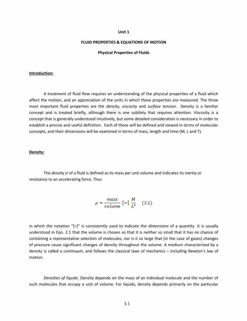
liquid and, to a much smaller extent, on its temperature. Representative densities are given in table 2.1.
The accuracy of the values given in tables 2.1 through 2.3 is adequate for the calculation needed for this
course. However, if highly accurate values are needed, particularly at extreme conditions, then
specialized information should be sought elsewhere.
Degrees A.P.I. (American Petroleum Institute) are related to specific gravity s by the formula:
Note that for water, oA.P.I. = 10, with correspondingly higher values for liquids that are less dense. Thus,
for the crude oil listed in table 2.1, Eqn. 2.2 indeed gives 141.5 / 0.851 – 131.5 = 35 oA.P.I.
Density of gases. For ideal gases, ρV = nRT, where p is the absolute pressure, V is the volume of
the gas, n is the number of moles, R is the gas constant, and T is the absolute temperature. If Mw is the
molecular weight of the gas, it follows:
Table 2.1
I-3
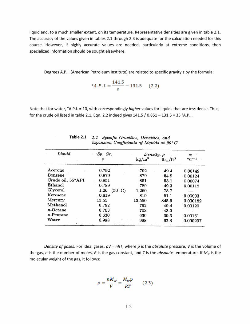
Thus, the density of an ideal gas depends on the molecular weight, absolute pressure, and absolute
temperature. Values of the gas constant R are given in table 2.2 for various systems of units. Note the
degrees Kelvin, formerly represented by “oK” is now more simply donated by “K”.
For a nonideal gas, the compressibility factor Z (a function of p and T) is introduced into the
denominator of Eqn. (2.3), giving:
Thus, the extent to which Z deviates from unity gives a measure of the nonideality of the gas.
The isothermal compressibility of a gas in defined as:
Table 2.2
I-4
and equals – at constant temperature – the fractional decrease in volume caused by a unit increase in
the pressure. For an ideal gas, β = 1 / p, the reciprocal of the absolute pressure.
The coefficient of thermal expansion α of a material is its isobaric fractional increase in volume
per unit rise in temperature:
Since, for a given mass, density is inversely proportional to volume, it follows that for moderate
temperature ranges (over which α is essentially constant) the density of most liquids is approximately a
linear function of temperature:
whereρo is the density at a reference temperature To. For an ideal gas, α = 1 / T, the reciprocal of the
absolute temperature.
The specific gravity s of a fluid is the ratio of the density ρ to the density ρsc of a reference fluid
at some standard condition:
For liquids, ρsc is usually the density of water at 4oC, which equals 1.000 g / ml or 1,000 kg / m3. For
gases, ρsc is sometimes taken as the density of air at 60oFand 14.7 psia, which is approximately 0.0759
lbm / ft3, and sometimes at 0oC and one atmosphere absolute; since there is no single standard for gases,
care must obviously be taken when interpreting published values. For natural gas, consisting primarily
I-5
of methane and other hydrocarbons, the gas gravity is defined as the ratio of the molecular weight of
the gas to that of air (28.8 lbm / lb-mole).
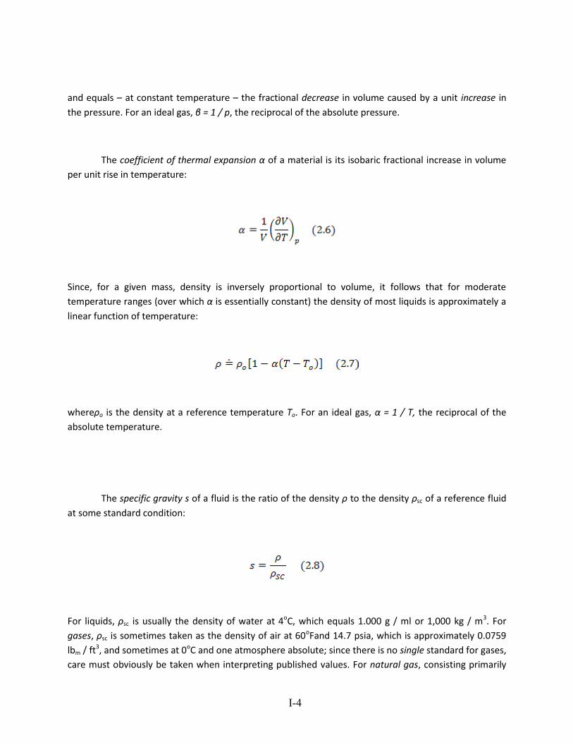
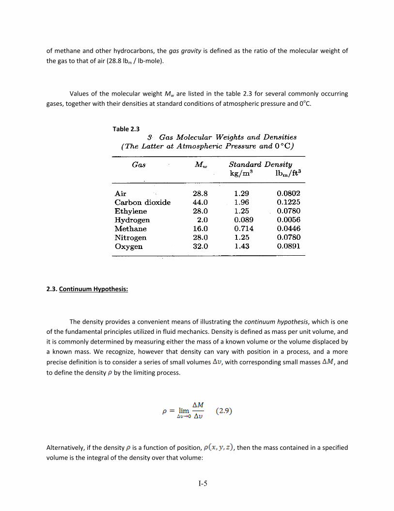
Values of the molecular weight Mw are listed in the table 2.3 for several commonly occurring
gases, together with their densities at standard conditions of atmospheric pressure and 0oC.
2.3. Continuum Hypothesis:
The density provides a convenient means of illustrating the continuum hypothesis, which is one
of the fundamental principles utilized in fluid mechanics. Density is defined as mass per unit volume, and
it is commonly determined by measuring either the mass of a known volume or the volume displaced by
a known mass. We recognize, however that density can vary with position in a process, and a more
precise definition is to consider a series of small volumes , with corresponding small masses , and
to define the density by the limiting process.
Alternatively, if the density is a function of position, , then the mass contained in a specified
volume is the integral of the density over that volume:
Table 2.3
I-6
Now, Eqns. 2.9 and 2.10 have implicitly used the continuum hypothesis, for they assume that the
density is a concept that has meaning for any volume, no matter how small. Yet we know that when the
volume is of molecular dimensions we have very rapid spatial variations between dense and non-dense
regions, depending on how close we are to a molecule. Hence, the notion of a density function that can
be defined by a limiting process such as that of Eqn. 2.9 is questionable. The continuum hypothesis
assumes that mathematical limits for volumes tending to zero are reached over a scale that remains
large compared to molecular dimensions. Thus, variations on a molecular scale can be ignored, since
they average out over all length scales of interest. Clearly, no result derived using the continuum
hypothesis should be expected to apply a rarified gas, where the distance between molecules may be
large.
2.4. Viscosity:
The viscosity is a measure of resistance to flow. It we tip over a glass of water on the table, the
water will spill out before we can stop it. If we tip over a jar of honey, we probably can set it upright
again before much honey flow out; this is because the honey has much greater resistance to flow, more
viscosity, than water. A more precise definition of viscosity is possible in terms of following experiment:
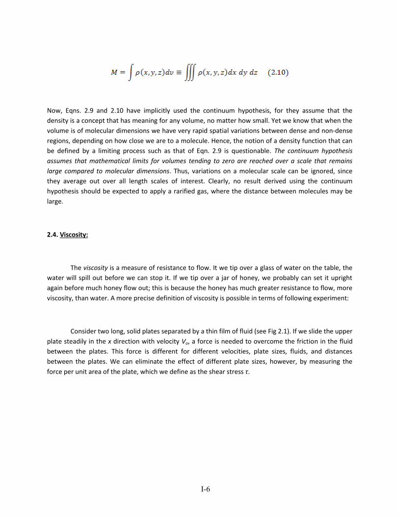
Consider two long, solid plates separated by a thin film of fluid (see Fig 2.1). If we slide the upper
plate steadily in the x direction with velocity Vo, a force is needed to overcome the friction in the fluid
between the plates. This force is different for different velocities, plate sizes, fluids, and distances
between the plates. We can eliminate the effect of different plate sizes, however, by measuring the
force per unit area of the plate, which we define as the shear stress τ.
I-7
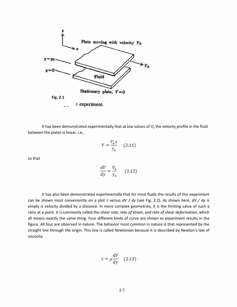
It has been demonstrated experimentally that at low values of Vo the velocity profile in the fluid
between the plates is linear, i.e.,
so that
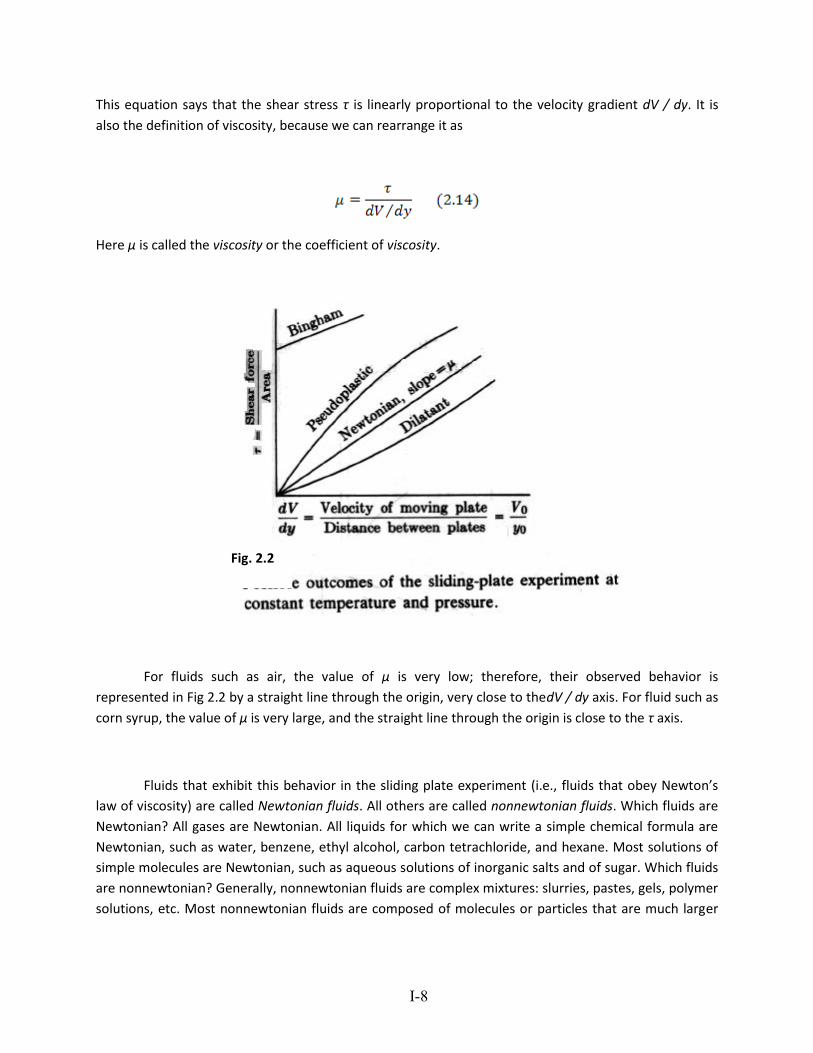
It has also been demonstrated experimentally that for most fluids the results of this experiment
can be shown most conveniently on a plot τ versus dV / dy (see Fig. 2.2). As shown here, dV / dy is
simply is velocity divided by a distance. In more complex geometries, it is the limiting value of such a
ratio at a point. It is commonly called the shear rate, rate of strain, and rate of shear deformation, which
all means exactly the same thing. Four different kinds of curve are shown as experiment results in the
figure. All four are observed in nature. The behavior most common in nature is that represented by the
straight line through the origin. This line is called Newtonian because it is described by Newton’s law of
viscosity
Fig. 2.1
I-8
This equation says that the shear stress τ is linearly proportional to the velocity gradient dV / dy. It is
also the definition of viscosity, because we can rearrange it as
Here μ is called the viscosity or the coefficient of viscosity.
For fluids such as air, the value of μ is very low; therefore, their observed behavior is
represented in Fig 2.2 by a straight line through the origin, very close to thedV / dy axis. For fluid such as
corn syrup, the value of μ is very large, and the straight line through the origin is close to the τ axis.
Fluids that exhibit this behavior in the sliding plate experiment (i.e., fluids that obey Newton’s
law of viscosity) are called Newtonian fluids. All others are called nonnewtonian fluids. Which fluids are
Newtonian? All gases are Newtonian. All liquids for which we can write a simple chemical formula are
Newtonian, such as water, benzene, ethyl alcohol, carbon tetrachloride, and hexane. Most solutions of
simple molecules are Newtonian, such as aqueous solutions of inorganic salts and of sugar. Which fluids
are nonnewtonian? Generally, nonnewtonian fluids are complex mixtures: slurries, pastes, gels, polymer
solutions, etc. Most nonnewtonian fluids are composed of molecules or particles that are much larger
Fig. 2.2
I-9
than water molecules, such as the sand grains in a mud or the collagen molecules in gelatin, which are
thousands or millions of times larger than water molecules.
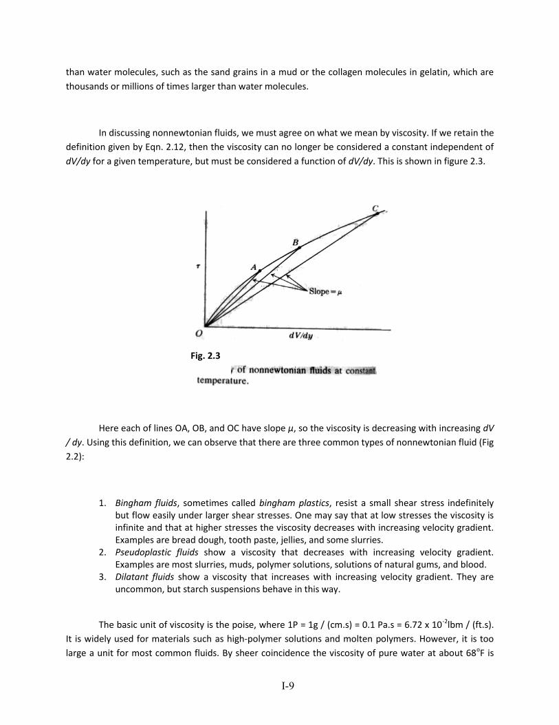
In discussing nonnewtonian fluids, we must agree on what we mean by viscosity. If we retain the
definition given by Eqn. 2.12, then the viscosity can no longer be considered a constant independent of
dV/dy for a given temperature, but must be considered a function of dV/dy. This is shown in figure 2.3.
Here each of lines OA, OB, and OC have slope μ, so the viscosity is decreasing with increasing dV
/ dy. Using this definition, we can observe that there are three common types of nonnewtonian fluid (Fig
2.2):
1. Bingham fluids, sometimes called bingham plastics, resist a small shear stress indefinitely but flow easily under larger shear stresses. One may say that at low stresses the viscosity is infinite and that at higher stresses the viscosity decreases with increasing velocity gradient. Examples are bread dough, tooth paste, jellies, and some slurries.
2. Pseudoplastic fluids show a viscosity that decreases with increasing velocity gradient. Examples are most slurries, muds, polymer solutions, solutions of natural gums, and blood.
3. Dilatant fluids show a viscosity that increases with increasing velocity gradient. They are uncommon, but starch suspensions behave in this way.
The basic unit of viscosity is the poise, where 1P = 1g / (cm.s) = 0.1 Pa.s = 6.72 x 10⁻²lbm / (ft.s).
It is widely used for materials such as high-polymer solutions and molten polymers. However, it is too
large a unit for most common fluids. By sheer coincidence the viscosity of pure water at about 68oF is
Fig. 2.3
I-10
0.01 P; for that reason the common unit of viscosity in the United States is the centipoises, where 1 cP =
0.01 P = 0.01 g / (cm.s) = 6.72 x 10⁻⁴lbm / (ft.s) = 0.001Pa.s. Hence, the viscosity of a fluid, expressed in
centipoises, is the same as the ratio of its viscosity to that of water at room temperature.
Kinematic Viscosity:
In many engineering problems, viscosity appears only in the relation of viscosity divided by density.
Therefore, to save writing, we define
The most common unit of kinematic viscosity is the centistokes (cSt):
(The kinematic viscosity of water at room temperature is 1cSt.) To avoid confusion over which viscosity
is being used , some writers refer to the viscosity μ as the absolute viscosity.
Surface Tension:
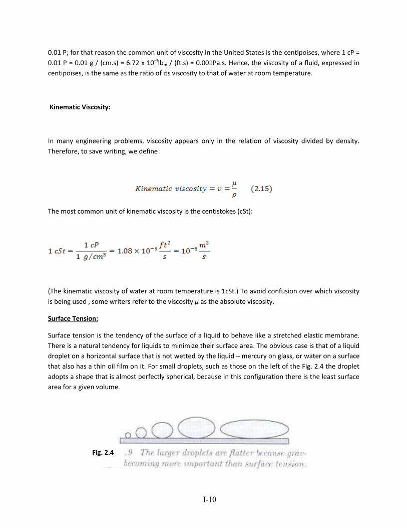
Surface tension is the tendency of the surface of a liquid to behave like a stretched elastic membrane.
There is a natural tendency for liquids to minimize their surface area. The obvious case is that of a liquid
droplet on a horizontal surface that is not wetted by the liquid – mercury on glass, or water on a surface
that also has a thin oil film on it. For small droplets, such as those on the left of the Fig. 2.4 the droplet
adopts a shape that is almost perfectly spherical, because in this configuration there is the least surface
area for a given volume.
Fig. 2.4
I-11
For larger droplets, the shape becomes somewhat flatter because of the increasingly important
gravitational effect, which is roughly proportional to , where a is the approximate droplet radius,
whereas the surface area is proportional only to . Thus, the ratio of gravitational to surface tension
effects depends roughly on the value of , and is therefore increasingly important for the
larger droplets, as shown to the right in the Fig 2.4. Overall, the situation is very similar to that of a
water-filled balloon, in which the water accounts for the gravitational effect and the balloon acts like the
surface tension.
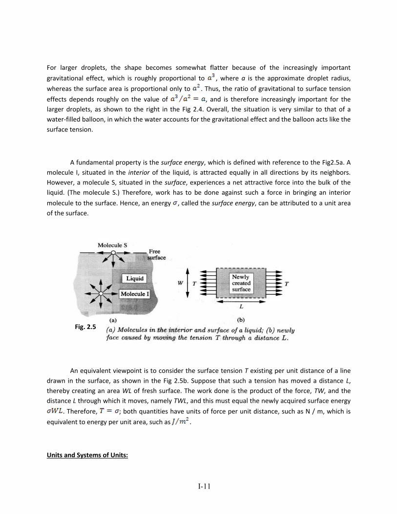
A fundamental property is the surface energy, which is defined with reference to the Fig2.5a. A
molecule I, situated in the interior of the liquid, is attracted equally in all directions by its neighbors.
However, a molecule S, situated in the surface, experiences a net attractive force into the bulk of the
liquid. (The molecule S.) Therefore, work has to be done against such a force in bringing an interior
molecule to the surface. Hence, an energy , called the surface energy, can be attributed to a unit area
of the surface.
An equivalent viewpoint is to consider the surface tension T existing per unit distance of a line
drawn in the surface, as shown in the Fig 2.5b. Suppose that such a tension has moved a distance L,
thereby creating an area WL of fresh surface. The work done is the product of the force, TW, and the
distance L through which it moves, namely TWL, and this must equal the newly acquired surface energy
. Therefore, ; both quantities have units of force per unit distance, such as N / m, which is
equivalent to energy per unit area, such as .
Units and Systems of Units:
Fig. 2.5
I-12
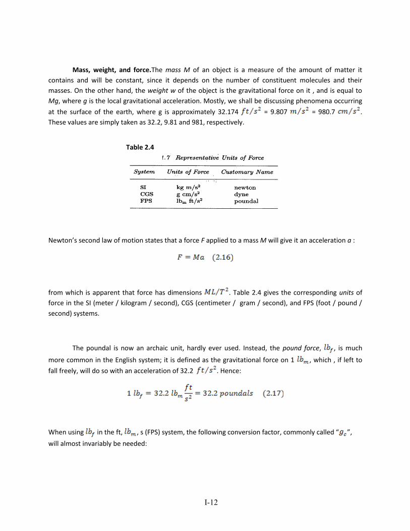
Mass, weight, and force.The mass M of an object is a measure of the amount of matter it
contains and will be constant, since it depends on the number of constituent molecules and their
masses. On the other hand, the weight w of the object is the gravitational force on it , and is equal to
Mg, where g is the local gravitational acceleration. Mostly, we shall be discussing phenomena occurring
at the surface of the earth, where g is approximately 32.174 = 9.807 = 980.7 .
These values are simply taken as 32.2, 9.81 and 981, respectively.
Newton’s second law of motion states that a force F applied to a mass M will give it an acceleration a :
from which is apparent that force has dimensions . Table 2.4 gives the corresponding units of
force in the SI (meter / kilogram / second), CGS (centimeter / gram / second), and FPS (foot / pound /
second) systems.
The poundal is now an archaic unit, hardly ever used. Instead, the pound force, , is much
more common in the English system; it is defined as the gravitational force on 1 , which , if left to
fall freely, will do so with an acceleration of 32.2 . Hence:
When using in the ft, , s (FPS) system, the following conversion factor, commonly called “ ”,
will almost invariably be needed:
Table 2.4
I-13
Some writers incorporate into their equations, but this approach may be confusing since it virtually
implies that one particular set of units is being use, and hence tends to rob the equations of their
generality. Why not, for example, also incorporate the conversion factor of 144 into equations
where pressure is expressed in ? We prefer to omit all conversion factors in equations, and
introduce them only as needed in evaluating expressions numerically. If the reader is in any doubt, units
should always be checked when performing calculations.
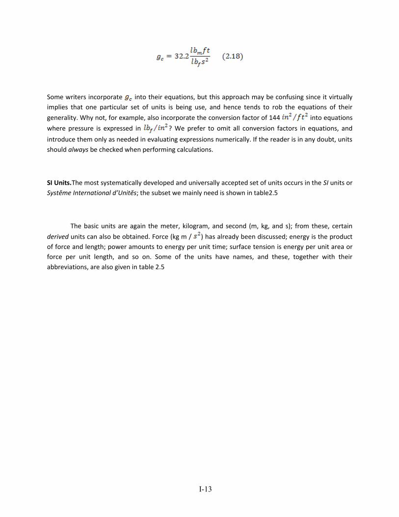
SI Units.The most systematically developed and universally accepted set of units occurs in the SI units or
Systĕme International d’Unitĕs; the subset we mainly need is shown in table2.5
The basic units are again the meter, kilogram, and second (m, kg, and s); from these, certain
derived units can also be obtained. Force (kg m / ) has already been discussed; energy is the product
of force and length; power amounts to energy per unit time; surface tension is energy per unit area or
force per unit length, and so on. Some of the units have names, and these, together with their
abbreviations, are also given in table 2.5
I-14
Tradition dies hard, and certain other “metric” units are so well established that they may be used as
auxiliary units; these are shown in table 2.6. The gram is the classic example. Note that the basic SI unit
of mass (kg) is even represented in terms of the gram, and has not yet been given a name of its own!
Table 2.5
Table 2.6
I-15
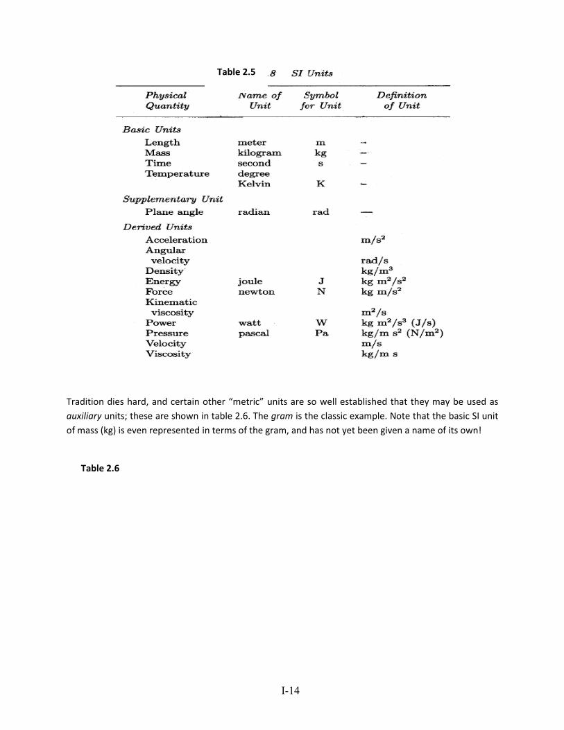
Table 2.7 shows some of the acceptable prefixes that can be used for accommodating both
small and large quantities. For example, to avoid an excessive number of decimal places, 0.000001 s is
normally better expressed as 1 (one microsecond). Note also , for example, that 1 should be
written as 1 mg-one prefix being better than two.
Some of the more frequently used conversion factors are given in the table
Example 2.1 – Units Conversion
Part 1.Express 65 mph in (a) , and (b)
Table 2.7
I-16
Solution:
(a)
(b)
Part 2. The density of 35 crude oil is 53.1 l at 68 and its viscosity is 32.8 .
What are its density, viscosity, and kinematic viscosity in SI units?
Solution:
Or, converting to SI units, noting that P is the symbol for poise, and evaluating v:
Example 2.2 – Mass of Air in a Room
I-17
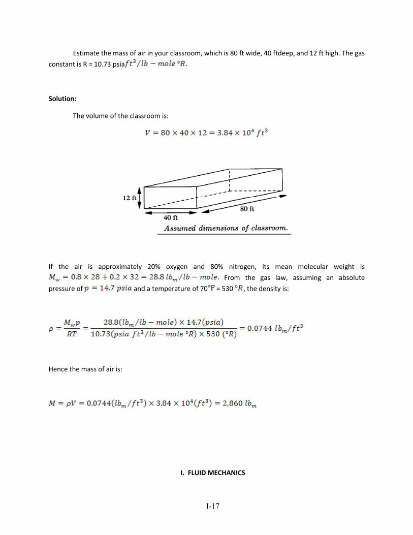
Estimate the mass of air in your classroom, which is 80 ft wide, 40 ftdeep, and 12 ft high. The gas
constant is R = 10.73 psia
Solution:
The volume of the classroom is:
If the air is approximately 20% oxygen and 80% nitrogen, its mean molecular weight is
From the gas law, assuming an absolute
pressure of and a temperature of 70 = 530 , the density is:
Hence the mass of air is:
I. FLUID MECHANICS
I-18
I.1 Basic Concepts & Definitions:
Fluid Mechanics - Study of fluids at rest, in motion, and the effects of fluids on
boundaries.
Note: This definition outlines the key topics in the study of fluids:
(1) fluid statics (fluids at rest), (2) momentum and energy analyses (fluids in motion), and (3) viscous effects and all sections considering pressure forces (effects of fluids on boundaries).
Fluid - A substance which moves and deformscontinuously as a result of an applied shear stress.
The definition also clearly shows that viscous effects are not considered in the study of fluid statics.
Two important properties in the study of fluid mechanics are:
Pressure and Velocity
These are defined as follows:
Pressure - The normal stress on any plane through a fluid element at rest.
Key Point: The direction of pressure forces will always be perpendicular to the
I-19
surface of interest.
Velocity - The rate of change of position at a point in a flow field. It is used not only to specify
flow field characteristics but also to specify flow rate, momentum, and viscous
effects for a fluid in motion.
I-20
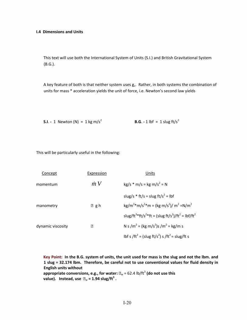
I.4 Dimensions and Units
This text will use both the International System of Units (S.I.) and British Gravitational System
(B.G.).
A key feature of both is that neither system uses gc. Rather, in both systems the combination of
units for mass * acceleration yields the unit of force, i.e. Newton’s second law yields
S.I. - 1 Newton (N) = 1 kg m/s2 B.G. - 1 lbf = 1 slug ft/s2
This will be particularly useful in the following:
Concept Expression Units
momentum Vm kg/s * m/s = kg m/s2 = N
slug/s * ft/s = slug ft/s2 = lbf
manometry g h kg/m3*m/s2*m = (kg m/s2)/ m2 =N/m2
slug/ft3*ft/s2*ft = (slug ft/s2)/ft2 = lbf/ft2
dynamic viscosity N s /m2 = (kg m/s2)s /m2 = kg/m s
lbf s /ft2 = (slug ft/s2) s /ft2 = slug/ft s
Key Point: In the B.G. system of units, the unit used for mass is the slug and not the lbm. and 1 slug = 32.174 lbm. Therefore, be careful not to use conventional values for fluid density in English units without appropriate conversions, e.g., for water: w = 62.4 lb/ft3 (do not use this value). Instead, use w = 1.94 slug/ft3 .
I-21
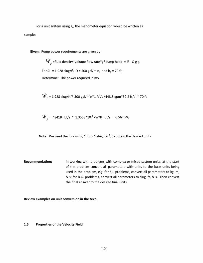
For a unit system using gc, the manometer equation would be written as
xample:
Given: Pump power requirements are given by
pW =fluid density*volume flow rate*g*pump head = Q g hp
For = 1.928 slug/ft3, Q = 500 gal/min, and hp = 70 ft,
Determine: The power required in kW.
pW = 1.928 slug/ft3* 500 gal/min*1 ft3/s /448.8 gpm*32.2 ft/s2 * 70 ft
pW = 4841ft–lbf/s * 1.3558*10-3 kW/ft–lbf/s = 6.564 kW
Note: We used the following, 1 lbf = 1 slug ft/s2, to obtain the desired units
Recommendation: In working with problems with complex or mixed system units, at the start
of the problem convert all parameters with units to the base units being
used in the problem, e.g. for S.I. problems, convert all parameters to kg, m,
& s; for B.G. problems, convert all parameters to slug, ft, & s. Then convert
the final answer to the desired final units.
Review examples on unit conversion in the text.
1.5 Properties of the Velocity Field
I-22
Two important properties in the study of fluid mechanics are:
Pressure and Velocity
The basic definition for velocity has been given previously. However, one of its most important
uses in fluid mechanics is to specify both the volume and mass flow rate of a fluid.
I-23
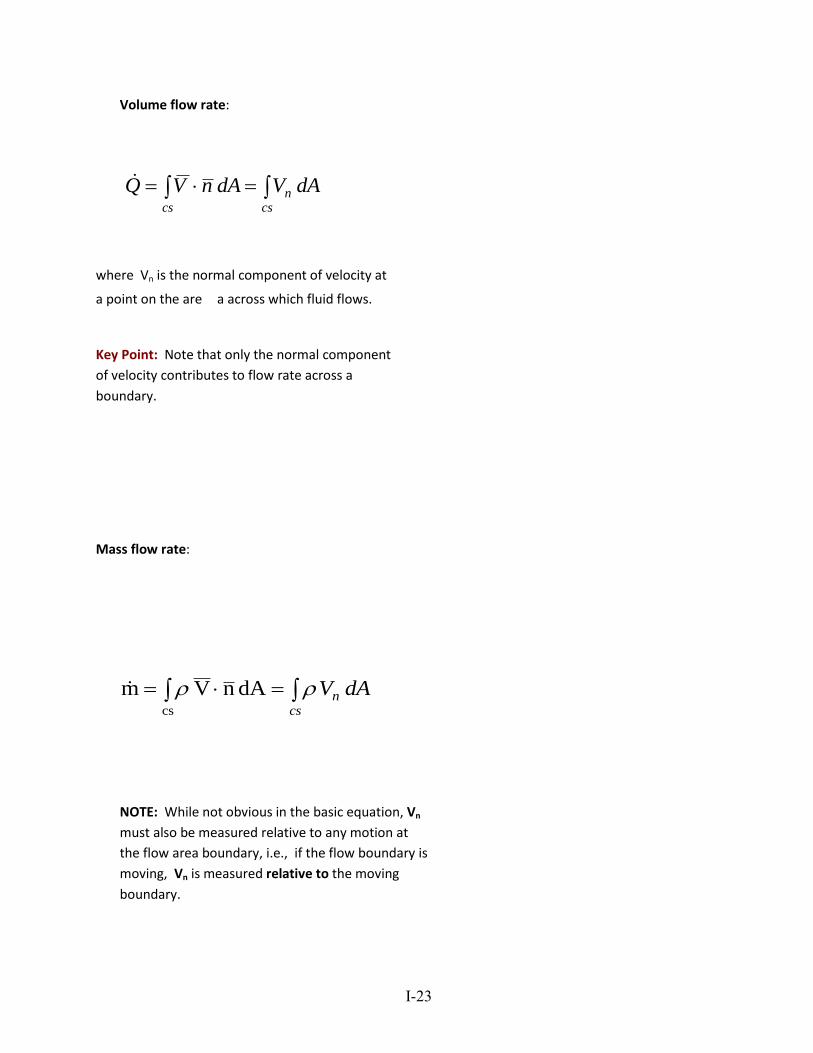
Volume flow rate:
cs cs
n dAVdAnVQ
where Vn is the normal component of velocity at
a point on the are a across which fluid flows.
Key Point: Note that only the normal component
of velocity contributes to flow rate across a
boundary.
Mass flow rate:
dAVcs
n cs
dAnVm
NOTE: While not obvious in the basic equation, Vn
must also be measured relative to any motion at
the flow area boundary, i.e., if the flow boundary is
moving, Vn is measured relative to the moving
boundary.
I-24
1.6 Thermodynamic Properties
All of the usual thermodynamic properties are important in fluid mechanics
P - Pressure (kPa, psi)
T- Temperature (oC, oF)
– Density (kg/m3, slug/ft3)
Alternatives for density
- specific weight = weight per unit volume (N/m3, lbf/ft3)
= g H2O: = 9790 N/m3 = 62.4 lbf/ft3
Air: = 11.8 N/m3 = 0.0752 lbf/ft3
S.G. - specific gravity = / (ref) where (ref) is usually at 4˚C, but some references will use
(ref) at 20˚C
liquids(ref) =(water at 1 atm, 4̊C) for liquids = 1000 kg/m3
gases(ref) = (air at 1 atm, 4˚C) for gases = 1.205 kg/m3
Example: Determine the static pressure difference indicated by an 18 cm column of fluid (liquid)
with a specific gravity of 0.85.
P = g h = S.G. ref h = 0.85* 9790 N/m3 0.18 m = 1498 N/m2 = 1.5 kPa
I-25
Ideal Gas Properties
Gases at low pressures and high temperatures have an equation-of-state ( the relationship between
pressure, temperature, and density for the gas) that is closely approximated by the ideal gas equation-
of-state.
The expressions used for selected properties for substances behaving as an ideal gas are given in the
following table.
I-26
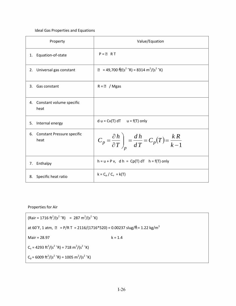
Ideal Gas Properties and Equations
Property Value/Equation
1. Equation-of-state P = R T
2. Universal gas constant = 49,700 ft2/(s2 ˚R) = 8314 m2/(s2 ˚K)
3. Gas constant R = / Mgas
4. Constant volume specific
heat
5. Internal energy d u = Cv(T) dT u = f(T) only
6. Constant Pressure specific
heat 1
k
RkTC
Td
hd
T
hC p
p
p
7. Enthalpy h = u + P v, d h = Cp(T) dT h = f(T) only
8. Specific heat ratio k = Cp / Cv = k(T)
Properties for Air
(Rair = 1716 ft2/(s2 ˚R) = 287 m2/(s2 ˚K)
at 60˚F, 1 atm, = P/R T = 2116/(1716*520) = 0.00237 slug/ft3 = 1.22 kg/m3
Mair = 28.97 k = 1.4
Cv = 4293 ft2/(s2 ˚R) = 718 m2/(s2 ˚K)
Cp = 6009 ft2/(s2 ˚R) = 1005 m2/(s2 ˚K)
I-27
I.7 Transport Properties
Certain transport properties are important as they relate to the diffusion of momentum due to shear
stresses. Specifically:
coefficient of viscosity (dynamic viscosity) {M / L t }
kinematic viscosity= / , L2 / t }
This gives rise to the definition of a Newtonian fluid.
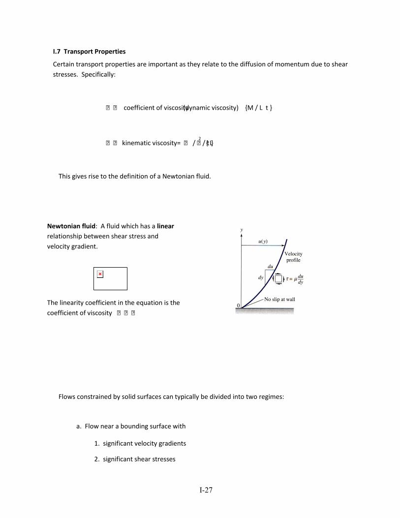
Newtonian fluid: A fluid which has a linear
relationship between shear stress and
velocity gradient.
The linearity coefficient in the equation is the
coefficient of viscosity
Flows constrained by solid surfaces can typically be divided into two regimes:
a. Flow near a bounding surface with
1. significant velocity gradients
2. significant shear stresses
I-28
This flow region is referred to as a "boundary layer."
b. Flows far from bounding surface with
1. negligible velocity gradients
2. negligible shear stresses
3. significant inertia effects
This flow region is referred to as "free stream" or "inviscid flow region."
I-29
An important parameter in identifying the characteristics of these flows is the
Reynolds number = Re
This physically represents the ratio of inertia forces in the flow to viscous forces. For most flows
of engineering significance, both the characteristics of the flow and the important effects due to
the flow, e.g., drag, pressure drop, aerodynamic loads, etc., are dependent on this parameter.
Surface Tension
Surface tension, Y, is a property important to the description of the interface between two fluids. The
dimensions of Y are F/L with units typically expressed as newtons/meter or pounds-force/foot. Two
common interfaces are water-air and mercury-air. These interfaces have the following values for
surface tension for clean surfaces at 20˚C (68˚F):
Contact Angle
For the case of a liquid interface intersecting a solid surface, the contact angle, , is a second important
parameter. For < 90˚, the liquid is said to ‘wet’ the surface; for> 90˚, this liquid is ‘non-wetting.’ For
example, water does not wet a waxed car surface and instead ‘beads’ the surface. However, water is
extremely wetting to a clean glass surface and is said to ‘sheet’ the surface.
Liquid Rise in a Capillary Tube
The effect of surface tension, Y, and contact angle, , can result in a liquid either rising or falling in a
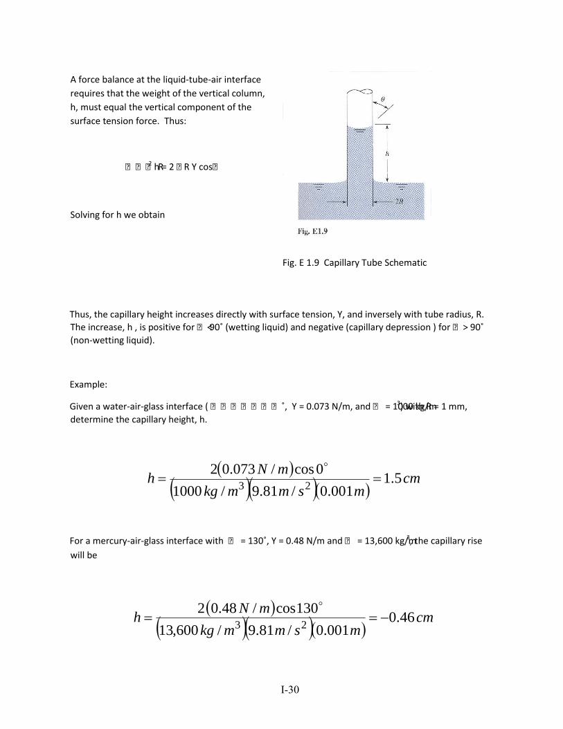
capillary tube. This effect is shown schematically in the Fig. E 1.9 on the following page.
I-30
A force balance at the liquid-tube-air interface
requires that the weight of the vertical column,
h, must equal the vertical component of the
surface tension force. Thus:
R2 h = 2 R Y cos
Solving for h we obtain
Fig. E 1.9 Capillary Tube Schematic
Thus, the capillary height increases directly with surface tension, Y, and inversely with tube radius, R.
The increase, h , is positive for < 90˚ (wetting liquid) and negative (capillary depression ) for > 90˚
(non-wetting liquid).
Example:
Given a water-air-glass interface ( ˚, Y = 0.073 N/m, and = 1000 kg/m3) with R = 1 mm,
determine the capillary height, h.
cm
msmmkg
mNh 5.1
001.0/81.9/1000
0cos/073.0223
For a mercury-air-glass interface with = 130˚, Y = 0.48 N/m and = 13,600 kg/m3, the capillary rise
will be
cm
msmmkg
mNh 46.0
001.0/81.9/600,13
130cos/48.0223
I-31
GOVERNING EQUATIONS OF FLUID DYNAMICS
I-32
1. GOVERNING EQUATIONS
1.1 Introduction
We are all familiar with fluids and we have all been fascinated at some time by fluid behavior: pouring, flowing, splashing and so on. At some level we have all built an intuitive understanding on how fluids behave.
Understanding fluid dynamics has been one of the major advances of physics, applied mathematics and engineering over the last hundred years. Starting with the explanations of aerofoil theory (i.e., why aircraft wings work), the study of fluids continues today with looking at how internal and surface waves, shock waves, turbulent fluid flow and the occurrence of chaos can be described mathematically. At the same time, it is important to realize how much of engineering depends on a proper understanding of fluids: from flow of water through pipes, to studying effluent discharge into the sea; from motions of the atmosphere, to the flow of lubricants in a car engine.
I-33
Fluid dynamics is also the key to our understanding of some of the most important phenomena in our physical world: ocean currents and weather systems, convection currents such as the motions of molten rock inside the Earth and the motions in the outer layers of the Sun, the explosions of supernovae and the swirling of gases in galaxies.
Like many fascinating subjects, understanding is not always easy. In particular, for fluid dynamics there are many terms and mathematical methods which will probably be unfamiliar. Although the basic concepts of velocity, mass, linear momentum, forces, etc., are the building blocks, the slippery nature of fluids means that applying those basic concepts sometimes takes some work.
Fluids can fascinate us exactly because they sometimes do unexpected things, which means we have to work harder at their mathematical explanation.
1.2 The continuity assumption
There are basically two ways of deriving the equations which governs the motion of a fluid. One of these methods approaches the question from the molecular point of view. The alternative method which is used to derive the equations which govern the motion of a fluid uses the continuum concept.
The continuity assumption considers fluids to be continuos. That is, properties such as density, pressure, temperature, and velocity are taken to be well-defined at infinitely small points, and are assumed to vary continuously from one point to another. The discrete, molecular nature of a fluid is ignored.
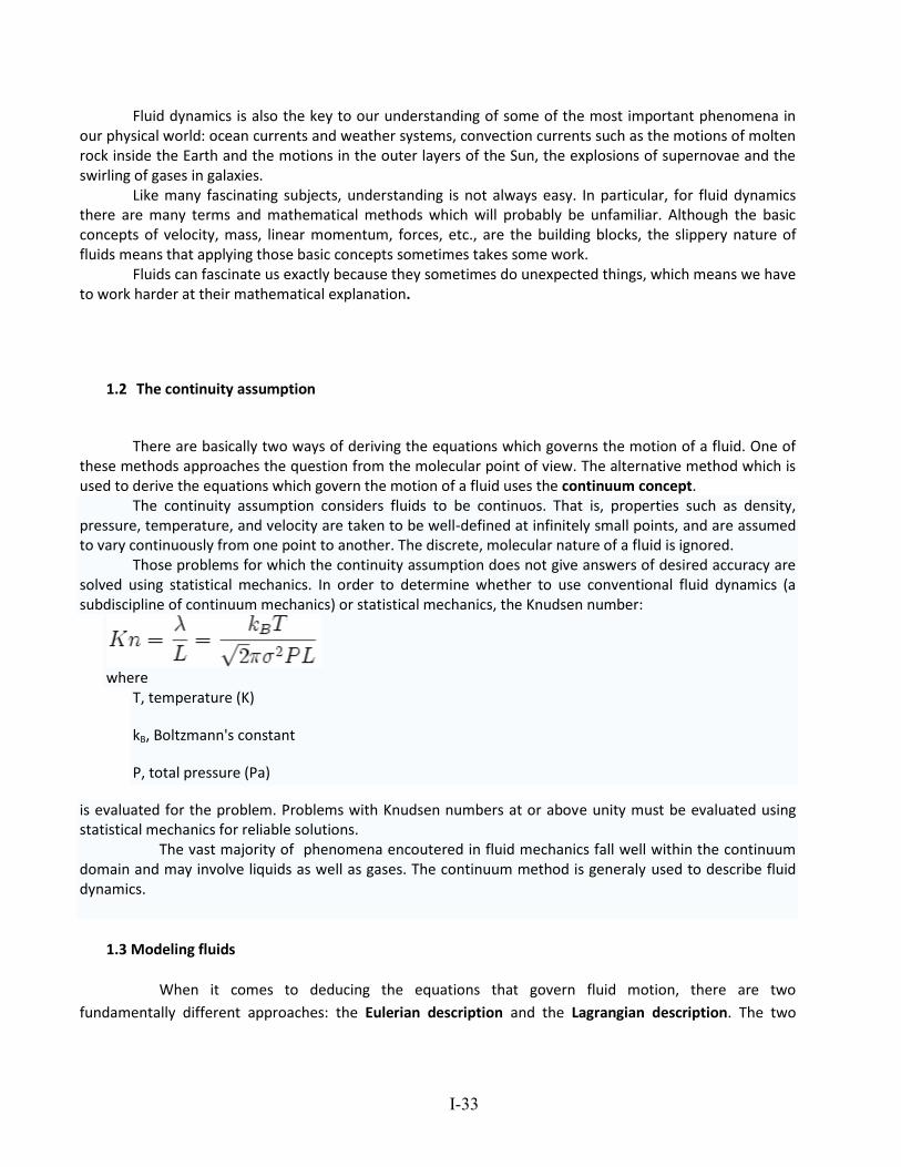
Those problems for which the continuity assumption does not give answers of desired accuracy are solved using statistical mechanics. In order to determine whether to use conventional fluid dynamics (a subdiscipline of continuum mechanics) or statistical mechanics, the Knudsen number:
where
T, temperature (K)
kB, Boltzmann's constant
P, total pressure (Pa)
is evaluated for the problem. Problems with Knudsen numbers at or above unity must be evaluated using statistical mechanics for reliable solutions. The vast majority of phenomena encoutered in fluid mechanics fall well within the continuum domain and may involve liquids as well as gases. The continuum method is generaly used to describe fluid dynamics.
1.3 Modeling fluids
When it comes to deducing the equations that govern fluid motion, there are two
fundamentally different approaches: the Eulerian description and the Lagrangian description. The two
I-34
viewpoints have been named in honor of the Swiss mathematician Leonhard Euler (1707–1783) and the
French mathematician and mathematical physicist Joseph-Louis Lagrange (1736-1813), respectively.
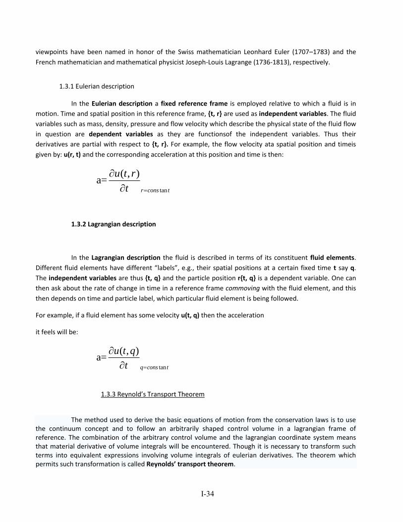
1.3.1 Eulerian description
In the Eulerian description a fixed reference frame is employed relative to which a fluid is in
motion. Time and spatial position in this reference frame, {t, r} are used as independent variables. The fluid
variables such as mass, density, pressure and flow velocity which describe the physical state of the fluid flow
in question are dependent variables as they are functionsof the independent variables. Thus their
derivatives are partial with respect to {t, r}. For example, the flow velocity ata spatial position and timeis
given by: u(r, t) and the corresponding acceleration at this position and time is then:
tan
( , )a=
r cons t
u t r
t
1.3.2 Lagrangian description
In the Lagrangian description the fluid is described in terms of its constituent fluid elements.
Different fluid elements have different “labels”, e.g., their spatial positions at a certain fixed time t say q.
The independent variables are thus {t, q} and the particle position r{t, q} is a dependent variable. One can
then ask about the rate of change in time in a reference frame commoving with the fluid element, and this
then depends on time and particle label, which particular fluid element is being followed.
For example, if a fluid element has some velocity u(t, q) then the acceleration
it feels will be:
tan
( , )a=
q cons t
u t q
t
1.3.3 Reynold’s Transport Theorem
The method used to derive the basic equations of motion from the conservation laws is to use the continuum concept and to follow an arbitrarily shaped control volume in a lagrangian frame of reference. The combination of the arbitrary control volume and the lagrangian coordinate system means that material derivative of volume integrals will be encountered. Though it is necessary to transform such terms into equivalent expressions involving volume integrals of eulerian derivatives. The theorem which permits such transformation is called Reynolds’ transport theorem.
I-35
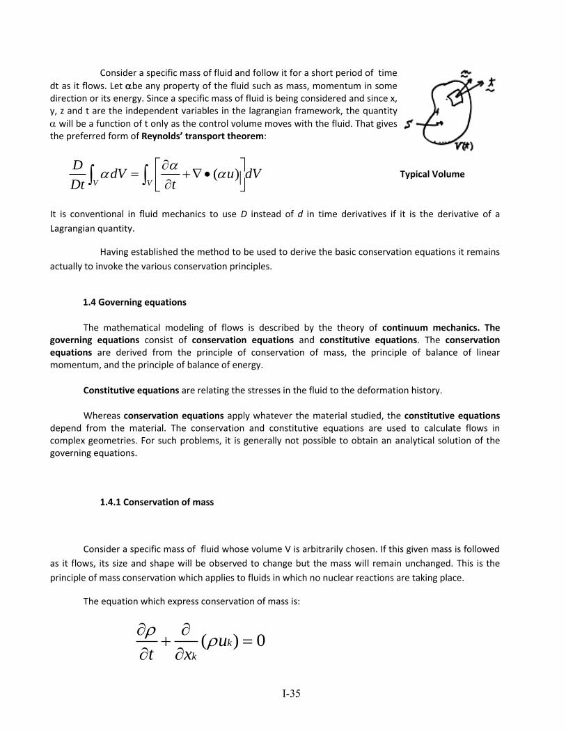
Consider a specific mass of fluid and follow it for a short period of time
dt as it flows. Let be any property of the fluid such as mass, momentum in some direction or its energy. Since a specific mass of fluid is being considered and since x, y, z and t are the independent variables in the lagrangian framework, the quantity
will be a function of t only as the control volume moves with the fluid. That gives the preferred form of Reynolds’ transport theorem:
( )V V
DdV u dV
Dt t
It is conventional in fluid mechanics to use D instead of d in time derivatives if it is the derivative of a
Lagrangian quantity.
Having established the method to be used to derive the basic conservation equations it remains
actually to invoke the various conservation principles.
1.4 Governing equations
The mathematical modeling of flows is described by the theory of continuum mechanics. The governing equations consist of conservation equations and constitutive equations. The conservation equations are derived from the principle of conservation of mass, the principle of balance of linear momentum, and the principle of balance of energy.
Constitutive equations are relating the stresses in the fluid to the deformation history.
Whereas conservation equations apply whatever the material studied, the constitutive equations depend from the material. The conservation and constitutive equations are used to calculate flows in complex geometries. For such problems, it is generally not possible to obtain an analytical solution of the governing equations.
1.4.1 Conservation of mass
Consider a specific mass of fluid whose volume V is arbitrarily chosen. If this given mass is followed
as it flows, its size and shape will be observed to change but the mass will remain unchanged. This is the
principle of mass conservation which applies to fluids in which no nuclear reactions are taking place.
The equation which express conservation of mass is:
( ) 0k
k
ut x
Typical Volume
I-36
The above equation express more than the fact that mass is conserved. Since it is a partial
differential equation, the implication is that the velocity is continuous. For this reason is usually called the
continuity equation.
In many practical cases of fluid flow the variation of density of the fluid may be ignored, for example
in most cases of the flow of liquids. In such cases the fluid is said to be incompressible, which means that as
a given mass of fluid is followed, not only will its mass be observed to remain constant but it’s volume and
hence its density.
Mathematically this special simplification of the continuity equation can be written as:
0D
Dt
or
0k
k
u
t x
Equation of continuity, either in the general form or the incompressible form is the first condition
which has to be satisfied by the velocity and the density of the fluid.
1.4.2 Conservation of momentum
The principle of conservation of momentum is in fact an application of Newton’s second law of
motion to an element of fluid. That is, when considering a given mass of fluid in a lagrangian frame of
reference, it is stated that the rate at which the momentum of the fluid mass is changing is equal to the net
external force acting on the mass. Thus the mathematical equation which results from imposing the physical
law of conservation of momentum is:
j j ijk i
k i
u uu f
t x x
where the left-hand side represents the rate of change of momentum of a unit the volume of fluid. The first
term is the familiar temporal acceleration term, while the second term is a convective acceleration and
allows for local accelerations (around obstacles) even when the flow is steady. This second term is also
nonlinear since the velocity appears quadratically. On the right hand side are the forces which are causing
the acceleration.
Fluid Forces There are two types:
surface forces (proportional to area)
body forces(proportional to volume)
Surface forces are usually expressed in terms of stress (= force per unit area):
I-37
force=stressarea
The major surface forces are:
pressure p: always acts normal to a surface
viscous stresses ij: frictional forces arising from relative motion of fluid layers. Body forces
The main body forces are:
gravity: the force per unit volume is
g= (0,0,-g)
(For constant-density fluids the effects of pressure and weight can be combined
in the governing equations as a piezometric pressure p* = p +gz)
Coriolis forces (in rotating reference frames). Separating surface forces (determined by a stress tensor ) and body forces (f per unit
volume), the integral equation for the i component of momentum may be written:
i i ij j i
V V V V
du dV u dA dA f dV
dt
surface forces body forces
1.4.3 Conservation of energy
The principle of conservation energy amounts to an application of the first law of thermodynamics to a fluid element as it flows. When applying the first law of thermodynamics to a flowing fluid the instantaneous energy of the fluid is considered to be the sum of the internal energy per unit mass and the kinetic energy per unit mass. In this way the modified form of the first law of thermodynamics which will be applied to an element of fluid states that the rate of change in the total energy (intrinsic plus kinetic) of the fluid as it flows is equal to the sum of the rate at which work is being done on the fluid by external forces and the rate on which heat is being added by conduction. In this way the mathematical expression becomes:
1( )
2V S V S
De u u dV uPdS u fdV q ndS
Dt
I-38
1.4.4 Constitutive equations
The basic conservation laws discussed in the previous section represent five scalar equations
which the fluid properties must satisfy as the fluid flows. The continuity and the energy equation are scalar
equations while the momentum equation is a vector which represents three scalar equations. But our basic
conservation laws have introduced seventeen unknowns: the scalars and e, the density and internal
energy respectively, the vectors uj and qj, the velocity and heat flux respectively, each vector having three
components and the stress tensor ij, which has in general nine independent components.
In order to obtain a complete set of equations the stress tensor ij and the heat-flux vector qj
must be further specified. This leads to so-called “constitutive equations” in which the stress tensor is
related to the deformation tensor and the heat-flux vector is related to the temperature gradients.
In order to achieve this end the postulates for a newtonian fluid are used. It should pointed out that
some fluid do not behave in a newtonian manner and their special characteristic are among the topics of
current research. One example is the class of fluids called viscoelastic fluids whose properties may be used
to reduce the drag of a body.
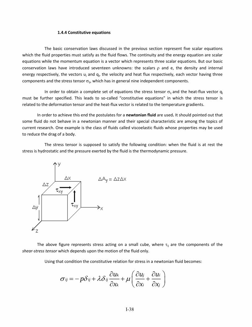
The stress tensor is supposed to satisfy the following condition: when the fluid is at rest the
stress is hydrostatic and the pressure exerted by the fluid is the thermodynamic pressure.
The above figure represents stress acting on a small cube, where ij are the components of the
shear-stress tensor which depends upon the motion of the fluid only.
Using that condition the constitutive relation for stress in a newtonian fluid becomes:
k j iij ij ij
k i j
u u up
x x x
I-39
The nine elements of the stress tensor have now been expressed in terms of the pressure and
the velocity gradients and two coefficients and . These coefficients cannot be determined analytically and
must be determined empirically. They are the viscosity coefficients of the fluid.
The second constitutive relation is Fourier’s Law for heat conduction:
j
j
Tq k
x
where qj is the heat-flux vector, k is the thermal conductivity of the fluid and T is the temperature.
1.4.5 Navier-Stokes Equations
The equation of momentum conservation together with the constitutive relation for a Newtonian
fluid yield the famous Navier-Stokes equations, which are the principal conditions to be satisfied by a fluid as
it flows:
j j k i jk
k j j k i j i
u u p u u uu f
t x x x x x x x
The Navier-Stokes equations for an incompressible fluid of constant density is:
2
2
j j jk i
k j i
u u p uu f
t x x x
In the special case of negligible viscous effects, Navier-Stokes equations become:
j jk i
k j
u u pu f
t x x
known as Euler equations.
1.4.6 In conclusion
the equations which govern the motion of a Newtonian fluid are:
I-40
The continuity equation:
0k
k
k k
uu
t x x
The Navier-Stokes equations:
j j k i jk
k j j k i j i
u u p u u uu f
t x x x x x x x
The energy equation
2k k j i j
k
k k k i j jj j
e e u T u u u uu p k
t x x x x x x x x
The thermal equation of state:
,p p T
The caloric equation of state:
( , )e e T
The above set of equations represents seven equation which are to be satisfied by seven
unknowns. Each of the continuity, energy and state equations supplies one scalar equation, while the
Navier-Stokes equation supplies three scalar equations. The seven unknowns are: the pressure (p), density
(), internal energy (e), temperature (T) and velocity components (uj). The parameters , and k are
assumed to be known from experimental data, and they may be constants or specified functions of the
temperature and pressure.
Useful concepts associated with the Bernoulli equation
- Static, Stagnation, and Dynamic Pressures
I-41
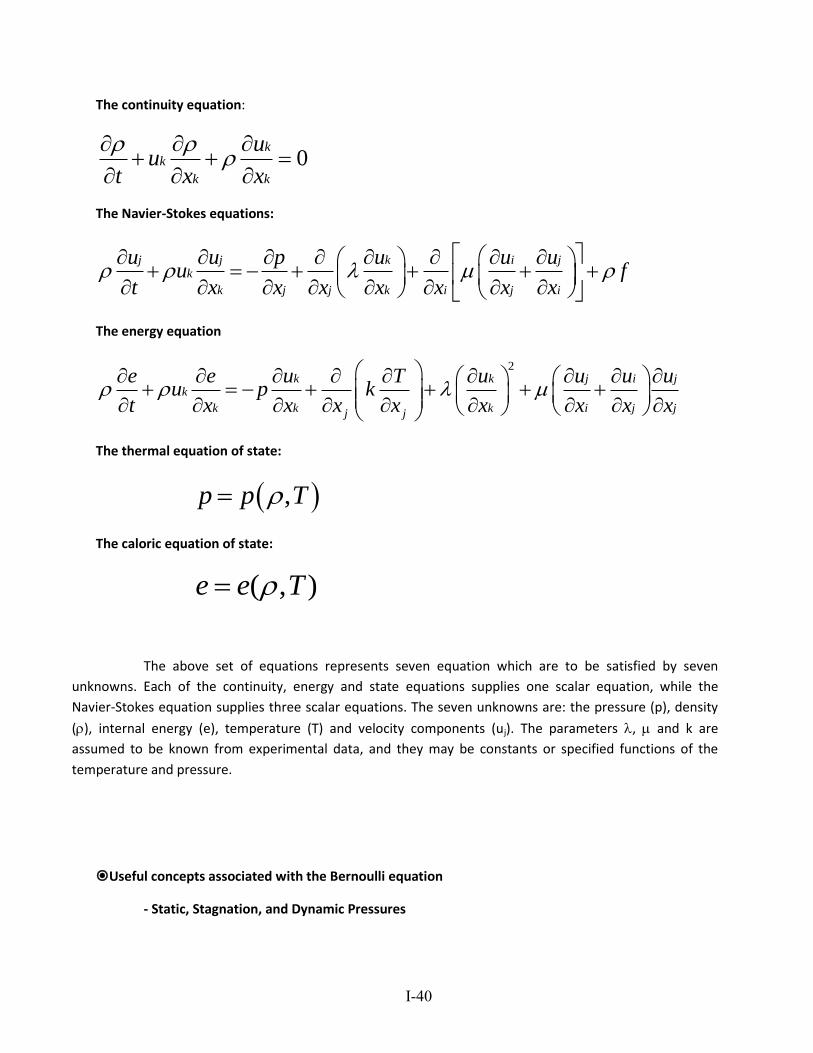
Bernoulli eq. along a streamline
constant (Unit of Pressure)
Physical meaning of each term
i) 1st term (Static pressure, p)
: Only due to the fluid weight
where (h4-3: Piezometer reading)
ii) 2nd term (Dynamic pressure,)
: Pressure increase or decrease due to fluid motion
iii) 3rd term (Gravitational potential,)
: Pressure change due to elevation change
Between Point (1) and Point (2) on the same streamline,
Difference in p between piezometer and tube inserted into a flow
(Stagnation pressure)
Piezometer
tube
Velocity of
stream
Static
(Thermodynamic)
Dynamic Hydrostatic
I-42
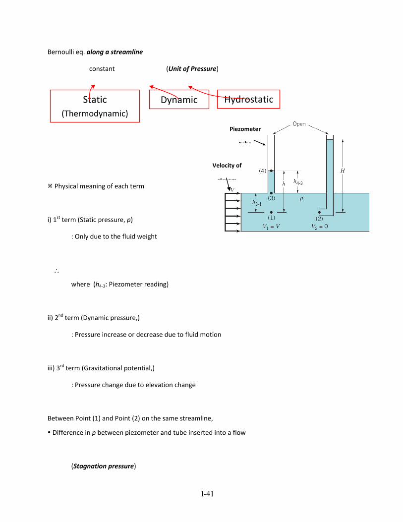
(Elevation change,: Due to dynamic pressure)
Point (2): Stagnation point ()
Line through point (2): Stagnation streamline
iv) Total pressure = constant (Along a streamline)
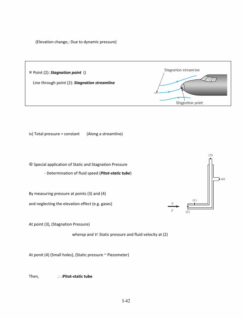
Special application of Static and Stagnation Pressure
- Determination of fluid speed (Pitot-static tube)
By measuring pressure at points (3) and (4)
and neglecting the elevation effect (e.g. gases)
At point (3), (Stagnation Pressure)
wherep and V: Static pressure and fluid velocity at (2)
At ponit (4) (Small holes), (Static pressure ~ Piezometer)
Then, :Pitot-static tube
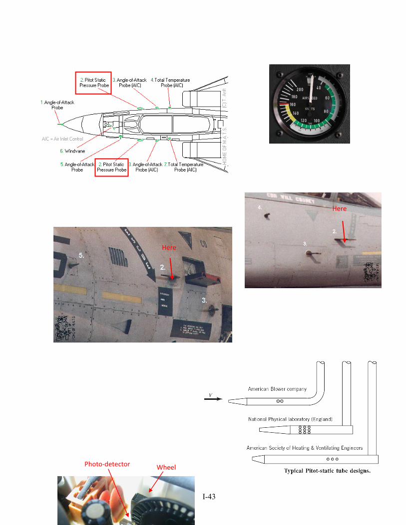
I-43
Wheel Photo-detector
Here
Here
I-44
How to use the Bernoulli equation (Examples)
Choose 2 points (1) and (2) along a streamline
: 6 variables
5 more conditions from the problem description
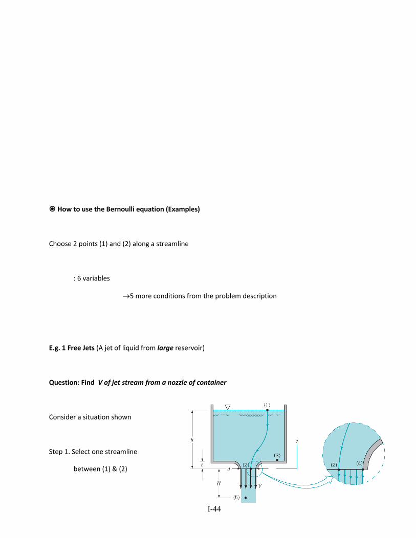
E.g. 1 Free Jets (A jet of liquid from large reservoir)
Question: Find V of jet stream from a nozzle of container
Consider a situation shown
Step 1. Select one streamline
between (1) & (2)
I-45
Step 2. Apply the Bernoulli eq.
between (1) & (2)
= 0 (Large container Negligible change of fluid level)
p2= 0 (Why?) [p2= p4 (Normal Bernoulli eq.)]
Then,
(If we choose z1 as h and z2 as 0)
or
hV
2gh2 : Velocity at the exit plane of nozzle
Velocity at any point [e.g. (5) in the figure] outside the nozzle,
(H: Distance from the nozzle)
: Conversion of P. E. to K.E. without viscosity (friction)
cf. Free body falling from rest without air resistance.
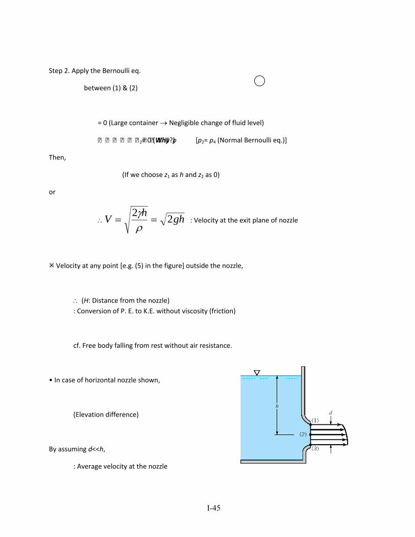
• In case of horizontal nozzle shown,
(Elevation difference)
By assuming d<<h,
: Average velocity at the nozzle
I-46
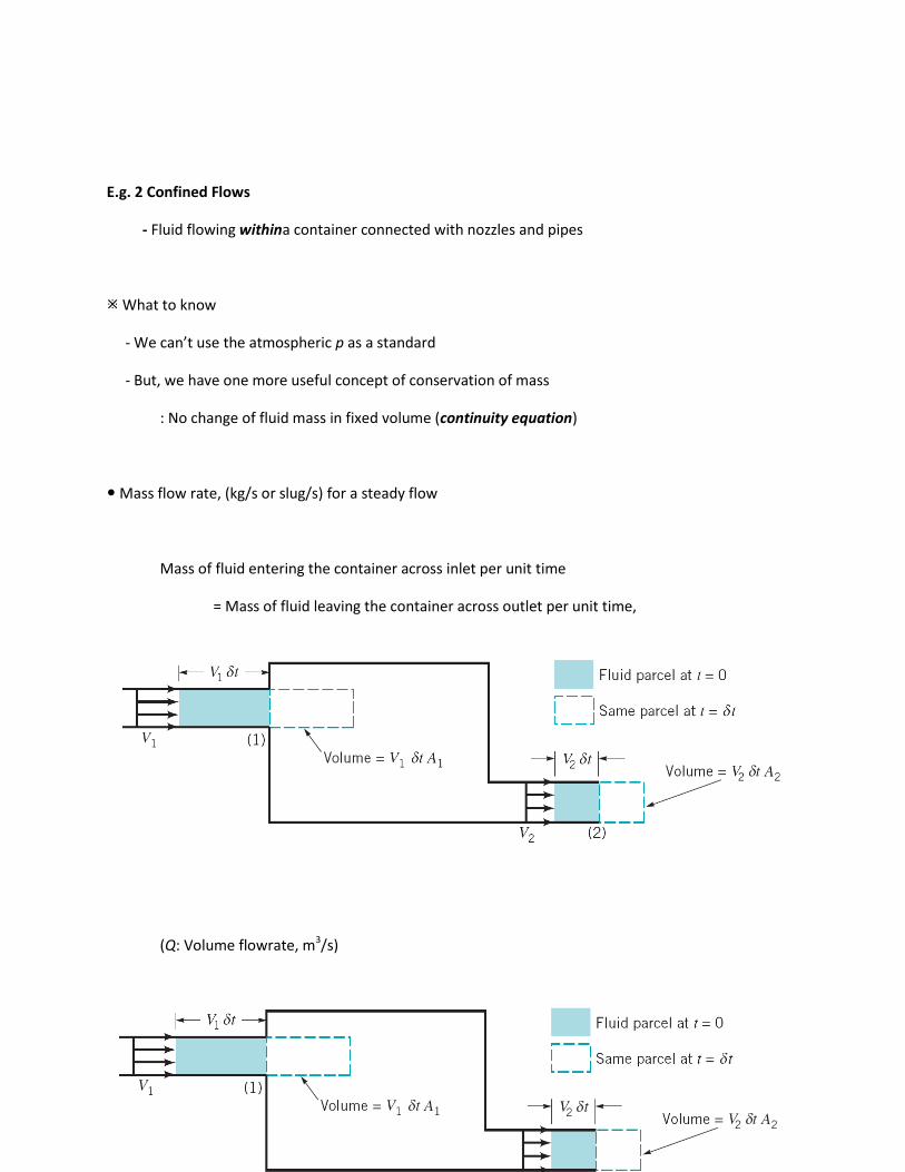
E.g. 2 Confined Flows
- Fluid flowing withina container connected with nozzles and pipes
What to know
- We can’t use the atmospheric p as a standard
- But, we have one more useful concept of conservation of mass
: No change of fluid mass in fixed volume (continuity equation)
Mass flow rate, (kg/s or slug/s) for a steady flow
Mass of fluid entering the container across inlet per unit time
= Mass of fluid leaving the container across outlet per unit time,
(Q: Volume flowrate, m3/s)
I-47
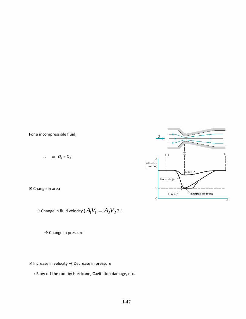
For a incompressible fluid,
or Q1 = Q2
Change in area
→ Change in fluid velocity ( 2211 VAVA )
→ Change in pressure
Increase in velocity → Decrease in pressure
: Blow off the roof by hurricane, Cavitation damage, etc.
I-48
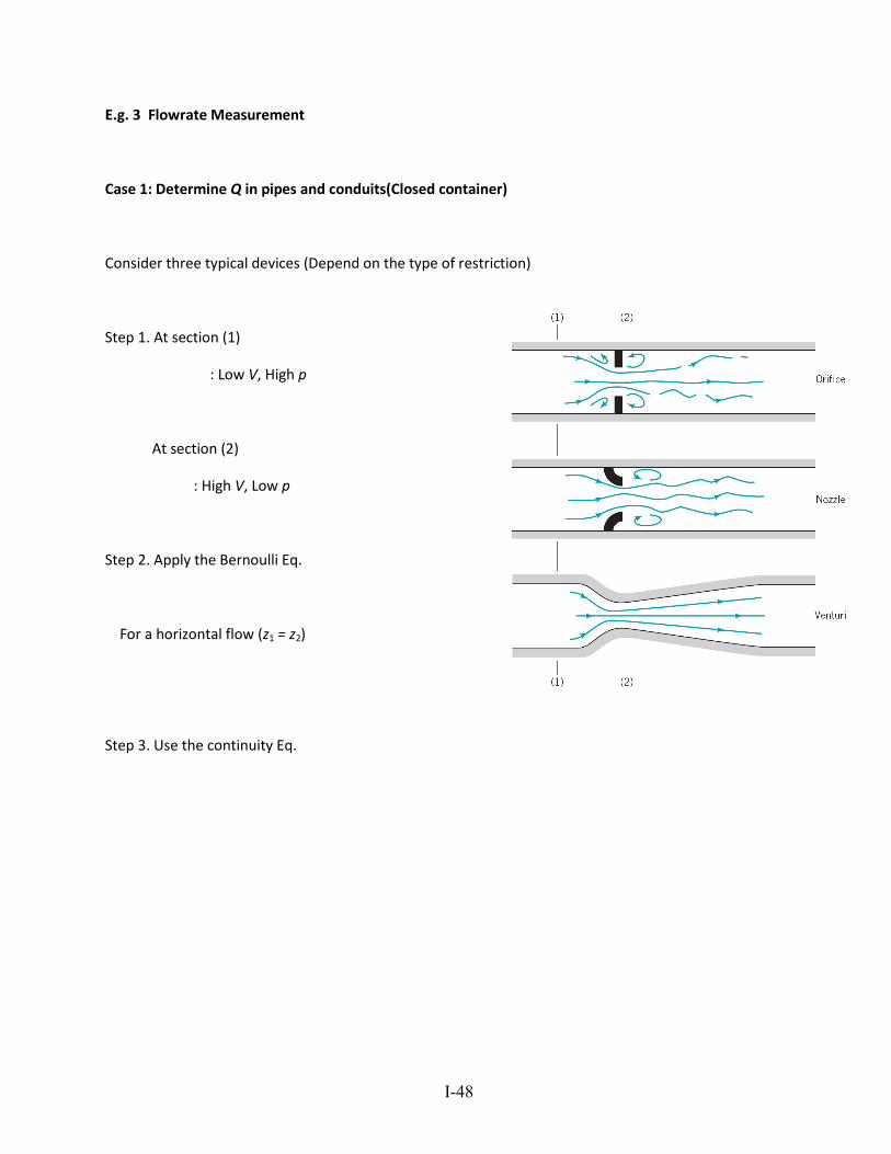
E.g. 3 Flowrate Measurement
Case 1: Determine Q in pipes and conduits(Closed container)
Consider three typical devices (Depend on the type of restriction)
Step 1. At section (1)
: Low V, High p
At section (2)
: High V, Low p
Step 2. Apply the Bernoulli Eq.
For a horizontal flow (z1 = z2)
Step 3. Use the continuity Eq.
I-49
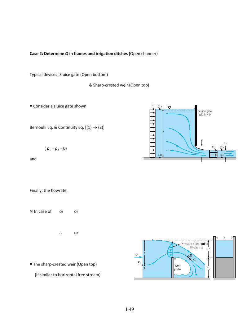
Case 2: Determine Q in flumes and irrigation ditches (Open channer)
Typical devices: Sluice gate (Open bottom)
& Sharp-crested weir (Open top)
Consider a sluice gate shown
Bernoulli Eq. & Continuity Eq. [(1) (2)]
( p1 = p2 = 0)
and
Finally, the flowrate,
In case of or or
or
The sharp-crested weir (Open top)
(If similar to horizontal free stream)
I-50
Then, Average velocity across the top of the weir gH2
Flow area for the weir Hb
Q = C1Hb gH2 = C1b H3/2 g2
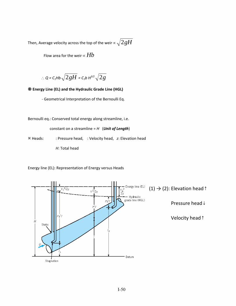
Energy Line (EL) and the Hydraulic Grade Line (HGL)
- Geometrical Interpretation of the Bernoulli Eq.
Bernoulli eq.: Conserved total energy along streamline, i.e.
constant on a streamline = H (Unit of Length)
Heads: : Pressure head, : Velocity head, z: Elevation head
H: Total head
Energy line (EL): Representation of Energy versus Heads
(1) → (2): Elevation head↑
Pressure head↓
Velocity head↑
(2) → (3): Elevation head ↑
Pressure head ↓
Velocity head ↑
I-51
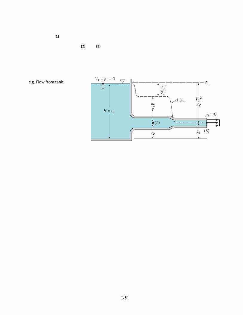
e.g. Flow from tank
(1)
(2) (3)
Recommended