Embed Size (px)
Citation preview

Equations of Motion and Variational Equations
MORE Relativity Working Group
16 Febbraio 2009
1 / 34

Contents
1. Introduction and Notation
2. Lagrangian formulation
3. Equations of motion and Variational equations:
Accelerations and Partial derivatives
3.1 Newtonian
3.2 General Relativity
3.3 PPN γ, β3.4 J2⊙ and variation of µ⊙
3.5 PPN α1, α2
4. Tests for partial derivatives
2 / 34

Notation
We will use the following notation:
−→r i = [x1i, x2i, x3i]
(−→r i)s = xs i
−→r i j = −→r j −−→r i
(−→r i j)s = xs j − xs i
ri j =| −→r i j | SSB
rirj
ri j
and an analogous notation hold for velocities −→v i = [x1i, x2i, x3i],where all the positions and velocities are with respect to the Solar
System Barycenter.
3 / 34

Equations of motion and Variational Equation
Let
X = F (X) X(0) = X0
be a generic Dynamical System with Flow ΦX0(t).
The Variational Equations for the System are:
d
dtA(t) =
∂ F
∂ X(ΦX0
(t)) A(t) A(0) = Id
where
A(t) =∂ΦX0
(t)
∂ X0
is needed for the Differential correction process.
4 / 34
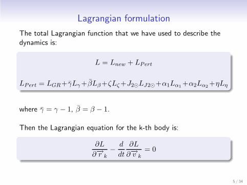
Lagrangian formulation
The total Lagrangian function that we have used to describe the
dynamics is:
L = Lnew + LPert
LPert = LGR+ γLγ +βLβ +ζLζ +J2⊙LJ2⊙+α1Lα1+α2Lα2
+ηLη
where γ = γ − 1, β = β − 1.
Then the Lagrangian equation for the k-th body is:
∂L
∂−→r k
−d
dt
∂L
∂−→v k
= 0
5 / 34

Lagrangian function components
The total Lagrangian function L is constituted by the Newtonian
n-body Lagrangian Lnew
Lnew =1
2
∑
i
µi v2
i +1
2
∑
i
∑
j 6=i
µiµj
rij
where the bodies considered are the Sun, Mercury, Earth, Moon,
Venus, Mars, Jupiter, Saturn, Uranus, Neptune and Pluto.
The perturbative Lagrangian functions are the following:
• General Relativity: LGR
• PPN γ, β: Lγ , Lβ
• Variation of µ⊙: Lζ
• Sun J2 effect: LJ2⊙
• Preferred frame effect: Lα1, Lα2
• Possible violation of the equivalence principle: Lη
6 / 34

Equations of motion
Let LP be any perturbative Lagrangian function, except the case
of Lη which has to be discussed separately, then the perturbative
acceleration of the k − th body can be calculated as in the
following.
If LP depends only on positions LP = LP (−→r ):
=⇒ −→akP =
1
µk
∂LP
∂−→rk
If LP depends also on velocities and LP = LP (−→r ,−→v ) = 1
c2L0
P :
=⇒ −→akP ∼=
1
µk
[
∂LP
∂−→rk
−
(
d
dt
∂LP
∂−→v k
)
∣
∣
∣
∣
∣−→a =−→a new
]
where −→a = −→a new because of O(c−2) approximation.
7 / 34

The Lagrangian formulation leads to the classic equations of
motion in the form
d
dt−→v k = −→a k
where
−→a k = −→a newk + −→a GR
k + γ−→a γk + β−→a β
k + ζ−→a ζk +
+J2⊙−→a
J2⊙
k + α1−→a α1
k + α2−→a α2
k + η−→a ηk +
−→P α
M
Note that the term−→P α/M is the apparent acceleration due to the
preferred frame effect, and it is the same for all bodies.
8 / 34

Variational equations
Once we have obtained the right hand side of the equations of motion,
we can solve also for the Variational equation:
∂−→a k
∂−→r l
∂−→a k
∂−→v l
which are the partial derivatives of the accelerations with respect to the
positions and the velocities.
In particular the ones that we need are the partial derivatives of the
accelerations of Mercury and of the Earth-Moon Barycenter, with respect
to the positions and velocities of Mercury, Earth and Moon.
In reality we also have to compute the derivatives of the acceleration of
the Sun because an indirect term is needed in the variational equations...
9 / 34

Indirect term due by the Sun in the Variational Equations
The Sun can be eliminated from the equations of motion by using
the origin in the Solar System Barycenter:
−→r0 = −
∑
i6=0µi−→r i
(
1 +v2
i
2 c2− Ui
2 c2
)
µ0
(
1 +v20
2 c2− U0
2 c2
)
where Ui =∑
k 6=iµk
rik.
So we have to consider the following indirect term in the partial
derivatives of the accelerations:
d−→a k
dxp l
=∂ −→a k
∂ xp l
+∂ −→a k
∂ xp 0
∂ xp 0
∂ xp l
d−→a k
d xp l
=∂ −→a k
∂ xp l
+∂ −→a k
∂ xp 0
∂ xp 0
∂ xp l
10 / 34

Newtonian part
The Classic Newtonian acceleration for the k-th body is:
−→a newk =
1
µk
∂Lnew
∂−→r k
=∑
i6=k
µi
r3
ki
−→r ki
The Partial derivatives with respect to positions and velocities are:
∂(−→aknew)s
∂xpl
=∑
i6=k
[
−3 µi
r5
ki
(−→r ki)p (−→r ki)s +µi
r3
ki
δps
]
(δl i − δlk)
∂(−→aknew)s
∂xpl
= 0
11 / 34

General Relativity Lagrangian function
The Lagrangian function taking into account the perturbation
terms due to General Relativity O(c−2) is:
LGR =1
8 c2
∑
i
µiv4
i +1
2
∑
i
∑
j 6=i
µi µj
rij
[
3
2c2(v2
i + v2
j ) +
−7
2 c2(−→vi ·
−→vj ) −1
2 c2(−→nij ·
−→vi )(−→nij ·
−→vj )
]
+
−1
2 c2
∑
i
∑
j 6=i
∑
k 6=i
µi µj µk
rij rik
where −→n i j = −→r i j/ri j .
12 / 34

General Relativity perturbative acceleration term
The perturbative acceleration due to General Relativity is:
−→a GRk =
1
c2
∑
j 6=k
µj
r3
kj
−→rkj
[
−4∑
l 6=k
µl
rkl
−∑
l 6=j
µl
rjl
+v2
k+2v2
j −4−→vk ·−→vj +
−3
2
(−→rjk · −→vj
rkj
)2
+1
2−→rkj ·
−→a newj
]
+1
c2
∑
j 6=k
µj
r3
kj
[−→rjk ·(4−→vk−3−→vj )]
−→vjk+
+7
2 c2
∑
j 6=k
µj
rkj
−→a newj
We don’t show the partial derivatives of −→a GRk with respect to
positions and velocities because of the length of these formulas!
13 / 34

Effect of GR perturbation on the orbit of Mercury
0 100 200 300 400 500 600 700 800−4
−3
−2
−1
0
1
2x 10
7 orbit perturbations Mercury, cm
time, days from arc beginning
red=
alon
g tr
ack,
gre
en=
radi
al, b
lack
=ou
t of p
lane
14 / 34

Effect of GR perturbation on the acceleration of Mercury
15 / 34

PPN γ and β Lagrangian functions
The Lagrangian functions taking into account the effect of PPN γand β are:
Lγ =1
2 c2
∑
i
∑
j 6=i
µi µj
ri j(−→vj −
−→vi )2
Lβ = −1
c2
∑
i
∑
j 6=i
∑
k 6=i
µi µj µk
rij rik
16 / 34

PPN parameters γ, β accelerations
The corresponding perturbative accelerations are:
−→a γk =
1
c2
∑
j 6=k
µj−→rkj
r3
kj
−2∑
l 6=k
µl
rkl
+ v2
k + v2
j − 2−→vk · −→vj
+
+2
c2
∑
j 6=k
µj
r3
kj
(−→rjk · −→vjk)−→vjk +
2
c2
∑
j 6=k
µj
rkj
−→a newj
−→a βk = −
2
c2
∑
j 6=k
µj
r3
kj
∑
l 6=k
µl
rkl
+∑
l 6=j
µl
rjl
−→rkj
17 / 34

Effect of γ on the orbit of Mercury for γ = 10−5
0 100 200 300 400 500 600 700 800−150
−100
−50
0
50
100orbit perturbations Mercury, cm
time, days from arc beginning
red=
alon
g tr
ack,
gre
en=
radi
al, b
lack
=ou
t of p
lane
18 / 34

Effect of γ on the acceleration of Mercury for γ = 10−5
19 / 34

Effect of β on the orbit of Mercury for β = 10−4
0 100 200 300 400 500 600 700 800−3000
−2500
−2000
−1500
−1000
−500
0
500orbit perturbations Mercury, cm
time, days from arc beginning
red=
alon
g tr
ack,
gre
en=
radi
al, b
lack
=ou
t of p
lane
20 / 34

Effect of β on the acceleration of Mercury for β = 10−4
21 / 34

Here we show the unfriendly formulas for the partial derivatives of
the accelerations due to γ:
∂ (−→a γk)
s
∂xp l
=2
c2
X
j 6=k
"
−
3µj
r5k j
(−→r k j)p (−→r k j)s +µj
r3k j
δp s
!
v2k j
2(δl j − δl k)+
+
−
µj
r3k j
(−→r k j)p
`
−→anewk j
´
s+
3 µj
r5k j
(−→r k j)p (−→r k j ·−→v k j) (−→v k j)s +
−
µj
r3k j
(−→v k j)p (−→v k j)s
!
(δl j − δl k) +µj
rk j
„
∂(−→a newj )s
∂xp l
−
∂(−→a newk )s
∂xp l
«
#
∂ (−→a γk)
s
∂xp l
=2
c2
X
j 6=k
"
µj
r3k j
“
(−→r k j)s (−→v k j)p − (−→r k j)p (−→v k j)s
”
+
−
µj
r3k j
(−→r k j ·−→v k j) δp s
#
(δl j − δl k)
22 / 34

. . . and β:
∂`
−→akβ´
s
∂xpl
= −
2
c2
X
j 6=k
"
−
µj
r5kj
“
−→r kj
”
p
“
−→r kj
”
s+
µi
r3kj
δps
!
“
δlj − δlk
”
·
·
X
h6=k
µh
rkh
+X
h6=j
µh
rjh
!#
+2
c2
X
j 6=k
µj
r3kj
“
−→r kj
”
s
"
X
h6=k
µh
r3kh
“
−→r kh
”
p
“
δlh − δlk
”
+
+X
h6=j
µh
r3jh
“
−→r jh
”
p
“
δlh − δlj
”
#
`
−→akβ´
s
∂xpl
= 0
23 / 34

Parameters ζ, J2⊙ Lagrangian functions
The Lagrangian Lζ takes into account the variation of the Sun
gravitational parameter µ⊙:
Lζ = (t − t0)∑
i6=0
µ0µi
r0i
The Lagrangian LJ2⊙ is the usual perturbation term due to the
oblateness of a body:
LJ2⊙ = −1
2
∑
i6=0
µ0 µi
r0 i
(
R0
r0 i
)2[
3 (−→n 0 i ·−→e 0)
2− 1
]
where −→e 0 is the unit vector along the rotation axis of the Sun.
24 / 34

Accelerations due to parameters ζ, J2⊙
For k 6= 0, i.e. a body different from the Sun, we have the
following perturbative accelerations:
−→a ζk = (t − t0)
µ0
r3
k0
−→r k0
−→aJ2⊙
k = −µ0 R2
0
2
[
−3
r5
0k
[3(−→n0k · −→e0)2 − 1]−→r0k +
+6
r4
0k
(−→n0k · −→e0)(−(−→n0k · −→e0)−→n0k + −→e0)
]
25 / 34

Effect of J2⊙ on the orbit of Mercury for J2⊙ = 10−8
0 100 200 300 400 500 600 700 800−200
0
200
400
600
800
1000
1200orbit perturbations Mercury, cm
time, days from arc beginning
red=
alon
g tr
ack,
gre
en=
radi
al, b
lack
=ou
t of p
lane
26 / 34

Effect of J2⊙ on the acceleration of Mercury for
J2⊙ = 10−8
27 / 34

PPN parameters α1, α2 Preferred frame effect
Lα1= −
1
4 c2
∑
j
∑
i6=j
µi µj
ri j
(−→z i ·−→z j)
Lα2=
1
4 c2
∑
j
∑
i6=j
µi µj
ri j[(−→z i ·
−→z j) − (−→ni j ·−→z i) (−→ni j ·
−→z j)]
where −→z i = −→v i + −→w and −→w is the velocity of the center of mass
of the solar system with respect to the preferred frame.
Note that we also have to take into account the apparent
acceleration−→P α/M, where M =
∑
i µi(1 +v2
i
2c2− Ui
2c2) and
−→P α = α1
∑
k
d
dt
∂Lα1
∂−→v k
+ α2
∑
k
d
dt
∂Lα2
∂−→v k
28 / 34
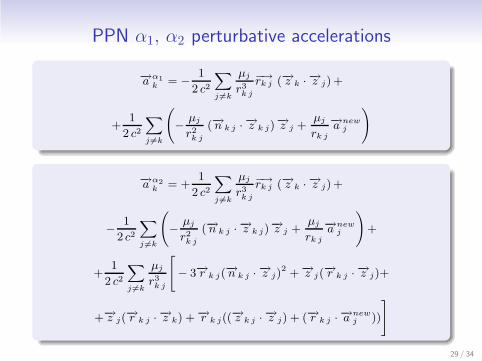
PPN α1, α2 perturbative accelerations
−→aα1
k = −
1
2 c2
X
j 6=k
µj
r3k j
−→rk j (−→z k ·−→z j) +
+1
2 c2
X
j 6=k
−
µj
r2k j
(−→n k j ·−→z k j)
−→z j +µj
rk j
−→anewj
!
−→aα2
k = +1
2 c2
X
j 6=k
µj
r3k j
−→rk j (−→z k ·−→z j) +
−
1
2 c2
X
j 6=k
−
µj
r2k j
(−→n k j ·−→z k j)
−→z j +µj
rk j
−→anewj
!
+
+1
2 c2
X
j 6=k
µj
r3k j
"
− 3−→r k j(−→n k j ·
−→z j)2 + −→z j(
−→r k j ·−→z j)+
+−→z j(−→r k j ·
−→z k) + −→r k j((−→z k j ·
−→z j) + (−→r k j ·−→a
newj ))
#
29 / 34

Effect of α1, α2 on the orbit of Mercury for
α1 = 8 × 10⁻⁶ α2 = 10
−6
0 100 200 300 400 500 600 700 800−3000
−2500
−2000
−1500
−1000
−500
0
500orbit perturbations Mercury, cm
time, days from arc beginning
red=
alon
g tr
ack,
gre
en=
radi
al, b
lack
=ou
t of p
lane
30 / 34

Effect of α1, α2 on the acceleration of Mercury for
α1 = 8 × 10⁻⁶ α2 = 10
−6
31 / 34

Partial derivatives of α1 acceleration...
∂ (−→a α1
k )s
∂xp l
= −
1
2 c2
X
j 6=k
"
−
3µj
r5k j
(−→r k j)p (−→r k j)s+µj
r3k j
δp s
#
(−→z k·−→z j)(δl j−δl k)+
+1
2 c2
X
j 6=k
"
3µj
r5k j
(−→r k j)p (−→r k j ·−→z k j) −
µj
r3k j
(−→z k j)p
#
(−→z j)s (δl j − δl k) +
+1
2 c2
X
j 6=k
"
−
µj
r3k j
(−→r k j)p (δl j − δl k)`
−→anewj
´
s+
µj
rk j
∂`
−→a newj
´
s
∂xp l
#
∂ (−→a α1
k )s
∂xp l
= −
1
2 c2
X
j 6=k
µj
r3k j
(−→r k j)s
“
δk l (−→z j)p + (−→z k)p δj l
”
+
+1
2 c2
X
j 6=k
−
µj
r3k j
(−→r k j)p (−→z j)s (δl j − δl k) −µj
r3k j
(−→r k j ·−→z k j) δp sδl j
!
32 / 34

...and very unfriendly partial derivatives of α2 acceleration:
∂“
−→aα2
k
”
s
∂xp l
=1
2 c2
X
j 6=k
2
4−3 µj
r5
k j
`−→r k j
´
p
`−→r k j
´
s+
µj
r3
k j
δp s
3
5
`−→z k · −→z j
´ `
δl j − δl k
´
+
−1
2 c2
X
j 6=k
2
4
3 µj
r5
k j
`−→r k j
´
p
`−→r k j · −→z k j
´
−µj
r3
k j
`−→z k j
´
p
3
5
`−→z j
´
s
`
δl j − δl k
´
+
−1
2 c2
X
j 6=k
2
6
4−
µj
r3
k j
`−→r k j
´
p
`
δl j − δl k
´
“
−→anewj
”
s+
µj
rk j
∂“
−→a newj
”
s
∂xp l
3
7
5
+1
2 c2
X
j 6=k
−3 µj
r5
k j
`−→r k j
´
p
`
δl j − δl k
´
"
− 3`−→r k j
´
s
`−→n k j · −→z j
´
2+
+`−→z j
´
s
`−→r k j · −→z j
´
+`−→z j
´
s
`−→r k j · −→z k
´
+`−→r k j
´
s
„
`−→z k j · −→z j
´
+
“
−→r k j · −→anewj
”
«
#
+
+1
2 c2
X
j 6=k
µj
r3
k j
"
− 3 δp s
`−→n k j · −→z j
´
2+ .........
33 / 34

Tests for partial derivatives formulas
In order to minimize the risk of errors in the computation of the
partial derivatives
LP −→ −→akP ∼=
1
µk
[
∂LP
∂−→rk
−
(
d
dt
∂LP
∂−→v k
)
∣
∣
∣
∣
∣−→a =−→a new
]
−→∂
(−→a Pk
)
s
∂xp l
,∂
(−→a Pk
)
s
∂xp l
we have tested the explicit, hand-calculated formulas, comparing
them with the ones obtained using the Maple symbolic toolbox.
In practice we have evaluated both the hand-calculated and the
computer-calculated formulas in some numerical values, and we
have compared the results.
34 / 34


![Reduction and reconstruction aspects of second-order dynamical … · • Lagrange-Poincar´e equations and reduction by stages [4, 13]; ... that is, equations derived by variational](https://img.pdfslide.net/doc/110x75/5fb2d1a0af961d4d91797191/reduction-and-reconstruction-aspects-of-second-order-dynamical-a-lagrange-poincare.jpg)