Unit - I
Computer vision Fundamentals
It is an area which concentrates on mimicking human vision systems. As a scientific discipline,
computer vision is concerned with the theory behind artificial systems that extract information
from images. The image data can take many forms, such as video sequences, views from
multiple cameras, or multi-dimensional data from a medical scanner.
As a technological discipline, computer vision seeks to apply its theories and models to the
construction of computer vision systems. Examples of applications of computer vision include
systems for:
• Controlling processes (e.g., an industrial robot).
• Navigation (e.g. by an autonomous vehicle or mobile robot).
• Detecting events (e.g., for visual surveillance or people counting).
• Organizing information (e.g., for indexing databases of images and image sequences).
• Modeling objects or environments (e.g., medical image analysis or topographical
modeling).
• Interaction (e.g., as the input to a device for computer-human interaction).
• Automatic inspection, e.g. in manufacturing applications
Sub-domains of computer vision include scene reconstruction, event detection, video tracking,
object recognition, learning, indexing, motion estimation, and image restoration.
In most practical computer vision applications, the computers are pre-programmed to solve a
particular task, but methods based on learning are now becoming increasingly common.
1. Fundamental steps in image processing:
1. Image acquisition: It is an area which acquires or converts a natural image to digital form so that it can be processed by a digital computer
2. Image Enhancement: It is an area which concentrates on modifying an image for a specific application. It improves the quality of the given image in ways that increase the
chances for success of the other processes. It is subjective, which means the
enhancement technique for one application may not be suitable for other applications.
3. Image Restoration: It is an area which concentrates on recovering or reconstructing or recovering an image that has been degraded by using a priori knowledge about the
degradation phenomena. also deals with improving the appearance of an image.
However, unlike enhancement, which is subjective, image restoration is objective, in the
sense that restoration techniques tend to be based on mathematical or probabilistic
models of image degradation. Enhancement, on the other hand, is based on human
subjective preferences regarding what constitutes a “good” enhancement result.
4. Image Compression: As the name implies, it deals with techniques for reducing the storage required to save an image, or the bandwidth required to transmit it. Although
storage technology has improved significantly over the past decade, the same cannot be
said for transmission capacity. This is true particularly in uses of the Internet, which are
characterized by significant pictorial content. Image compression is familiar (perhaps
inadvertently) to most users of computers in the form of image file extensions, such as
the jpg file extension used in the JPEG (Joint Photographic Experts Group) image
compression standard.
5. Image segmentation: It is an area which concentrates on isolating or grouping homogenous areas in an image. It divides the given image into its constituent parts or
objects.
6. Image representation: It is an area which concentrates on extracting the features from a given image and storing it in the memory. It converts the input image to a form that is
suitable for computer processing.
7. Image recognition: It is an area which concentrates on identifying an object from the given image. It assigns a label to an object based on the information provided by its
descriptors.
8. Image interpretation: to assign meaning to an ensemble of recognized objects.
9. Knowledge base : Knowledge about a problem domain is coded into an image processing system in the form of a knowledge database. This knowledge database is used
in all the areas
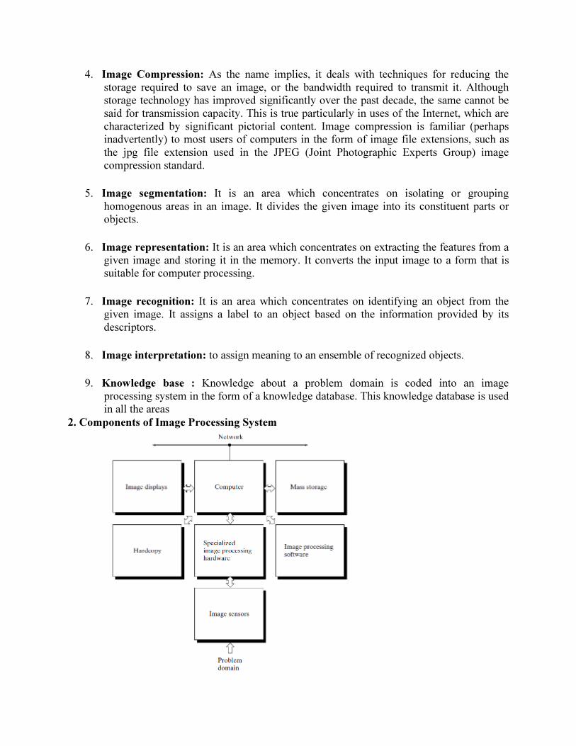
2. Components of Image Processing System
The above figure shows the basic components comprising a typical general-purpose system used
for digital image processing. The components includes Image displays Computer Mass storage,
Hardcopy, Specialized image processing hardware, Image sensors, Image processing software
and Problem domain
Image Sensors: With reference to sensing, two elements are required to acquire digital images.
The first is a physical device that is sensitive to the energy radiated by the object we wish to
image. The second, called a digitizer, is a device for converting the output of the physical
sensing device into digital form. For instance, in a digital video or Image camera, the sensors
produce an electrical output proportional to light intensity. The digitizer converts these outputs to
digital data
Specialized image processing hardware: It usually consists of the digitizer just mentioned, plus
hardware that performs other primitive operations, such as an arithmetic logic unit (ALU), which
performs arithmetic and logical operations in parallel on entire images. One example of how an
ALU is used is in averaging images as quickly as they are digitized, for the purpose of noise
reduction.
Computer: The computer in an image processing system is a general-purpose computer and can
range from a PC to a supercomputer. In dedicated applications, sometimes specially designed
computers are used to achieve a required level of performance, but our interest here is on
general-purpose image processing systems. In these systems, almost any well-equipped PC-type
machine is suitable for offline image processing tasks.
Software : It consists of specialized modules that perform specific tasks. A well-designed
package also includes the capability for the user to write code that, as a minimum, utilizes the
specialized modules. More sophisticated software packages allow the integration of those
modules and general- purpose software commands from at least one computer language.
Mass storage capability is a must in image processing applications. An image of size 1024*1024
pixels, in which the intensity of each pixel is an 8-bit quantity, requires one megabyte of storage
space if the image is not compressed. When dealing with thousands, or even millions, of images,
providing adequate storage in an image processing system can be a challenge.
Image displays in use today are mainly color (preferably flat screen) TV monitors. Monitors are
driven by the outputs of image and graphics display cards that are an integral part of the
computer system.
Hardcopy devices for recording images include laser printers, film cameras, heat-sensitive
devices, inkjet units, and digital units, such as optical and CD-ROM disks.
Networking : It is almost a default function in any computer system in use today. Because of the
large amount of data inherent in image processing applications, the key consideration in image
transmission is bandwidth. In dedicated networks, this typically is not a problem, but
communications with remote sites via the Internet are not always as efficient.
Basic Geometric Transformations Transformation is an operation which alters the position, size and shape of an object. It includes
translation, rotation, scaling, reflection, shear etc. these transformations are very important in the
fields of computer graphics and Computer vision. Basic transformations are translation, rotation,
scaling.
Translation: It is an operation which alters the position of an object. Equation of translation is
defined by
'
xx x t= + '
yy y t= +
Where (x , y) is the intial co-ordinates and (x’, y’) is the output co-ordinates and xt and
yt are the
translation distances respectively in x and y directions. The homogenous matrix representation
for translation is defined by
[ ] [ ]
x y
1 0 0
x', y',1 x, y,1 0 1 0
t t 0
= ×
Here
x y
1 0 0
0 1 0
t t 0
is known as translation matrix.
Rotations alter the orientation of an object: They are a little more complex than scales. Starting
in two dimensional rotations is easiest.
Rotations
A rotation moves a point along a circular path centered at the origin (the pivot). Equation of
Rotation is defined by
We express the rotation in matrix form as
Here
is the rotation matrix.
Scaling: It is an operation which alters the size of an object. Equation of scaling is defined by
'
xx x . S= '
yy y . S=
Where (x , y) is the intial co-ordinates and (x’, y’) is the output co-ordinates and xS and
yS are
the scaling factors respectively in x and y directions. The homogenous matrix representation for
Scaling is defined by
[ ] [ ]x
y
S 0 0
x', y',1 x, y,1 0 S 0
1 1 0
= ×
Here x
y
S 0 0
0 S 0
1 1 0
is known as Scaling matrix.
Reflection: It is an operation which gives the mirror effect to an object with respect to axis.
Shear: It is an operation which gives the parabolic effect to an object with respect to axis.
Image Digitization
Image : It is a two dimention light intensity function f(x, y) characterized by two components:
(1) the amount of source illumination incident on the scene being viewed, and (2) the amount of
illumination reflected by the objects in the scene. Appropriately, these are called the illumination
and reflectance components and are denoted by i(x, y) and r(x, y), respectively.The two
functions combine as a product to form f(x, y):
f(x, y)=i(x, y) . r(x, y)
where
0<i(x, y)< α
and
0<r(x, y)<=1
Equations indicates that reflectance is bounded by 0 (total absorption) and 1 (total
reflectance).The nature of i(x, y) is determined by the illumination source, and r(x, y) is
determined by the characteristics of the imaged objects. It is noted that these expressions also are
applicable to images formed via transmission of the illumination through a medium, such as a
chest X-ray.
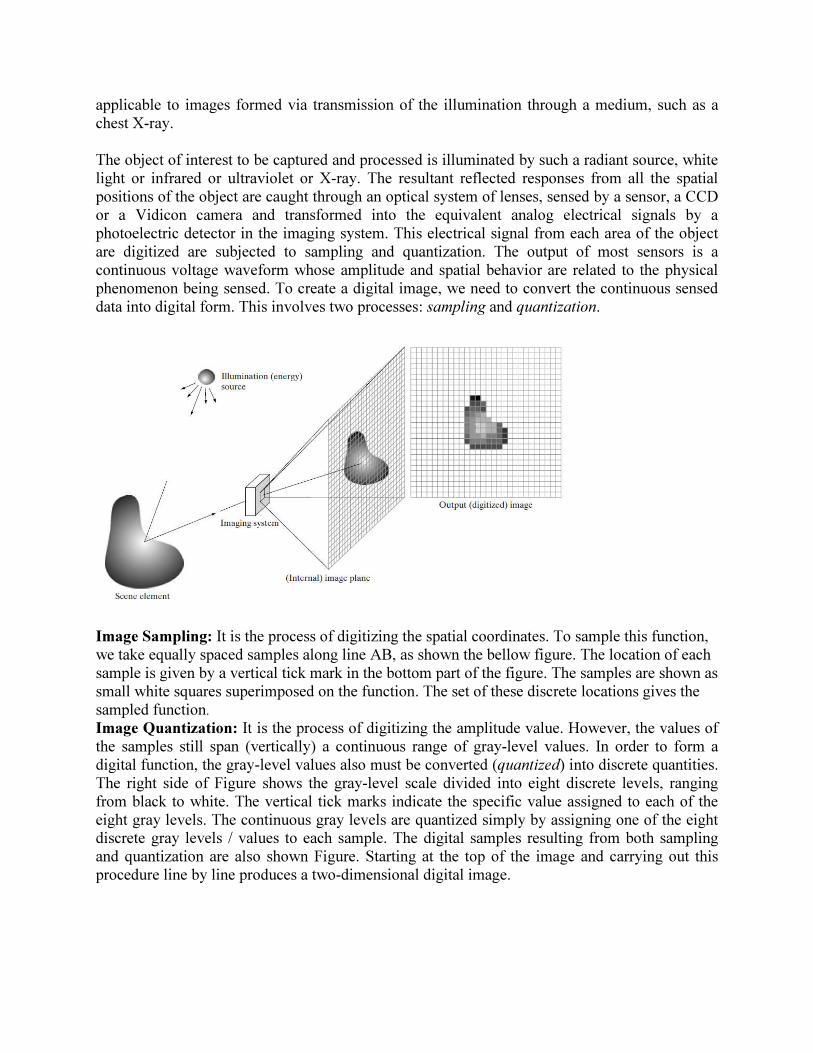
The object of interest to be captured and processed is illuminated by such a radiant source, white
light or infrared or ultraviolet or X-ray. The resultant reflected responses from all the spatial
positions of the object are caught through an optical system of lenses, sensed by a sensor, a CCD
or a Vidicon camera and transformed into the equivalent analog electrical signals by a
photoelectric detector in the imaging system. This electrical signal from each area of the object
are digitized are subjected to sampling and quantization. The output of most sensors is a
continuous voltage waveform whose amplitude and spatial behavior are related to the physical
phenomenon being sensed. To create a digital image, we need to convert the continuous sensed
data into digital form. This involves two processes: sampling and quantization.
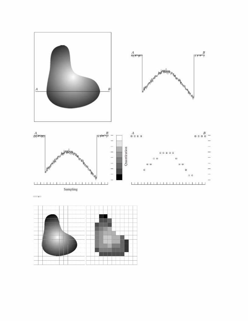
Image Sampling: It is the process of digitizing the spatial coordinates. To sample this function,
we take equally spaced samples along line AB, as shown the bellow figure. The location of each
sample is given by a vertical tick mark in the bottom part of the figure. The samples are shown as
small white squares superimposed on the function. The set of these discrete locations gives the
sampled function.
Image Quantization: It is the process of digitizing the amplitude value. However, the values of
the samples still span (vertically) a continuous range of gray-level values. In order to form a
digital function, the gray-level values also must be converted (quantized) into discrete quantities.
The right side of Figure shows the gray-level scale divided into eight discrete levels, ranging
from black to white. The vertical tick marks indicate the specific value assigned to each of the
eight gray levels. The continuous gray levels are quantized simply by assigning one of the eight
discrete gray levels / values to each sample. The digital samples resulting from both sampling
and quantization are also shown Figure. Starting at the top of the image and carrying out this
procedure line by line produces a two-dimensional digital image.
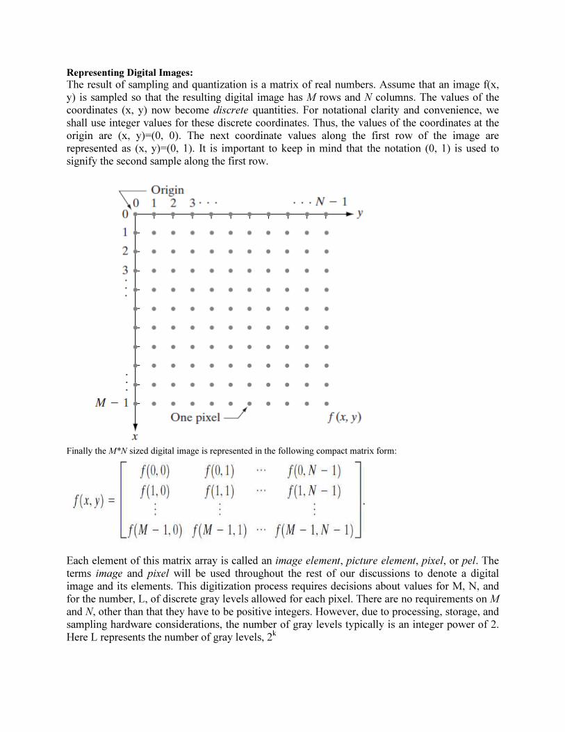
Representing Digital Images:
The result of sampling and quantization is a matrix of real numbers. Assume that an image f(x,
y) is sampled so that the resulting digital image has M rows and N columns. The values of the
coordinates (x, y) now become discrete quantities. For notational clarity and convenience, we
shall use integer values for these discrete coordinates. Thus, the values of the coordinates at the
origin are (x, y)=(0, 0). The next coordinate values along the first row of the image are
represented as (x, y)=(0, 1). It is important to keep in mind that the notation (0, 1) is used to
signify the second sample along the first row.
Finally the M*N sized digital image is represented in the following compact matrix form:
Each element of this matrix array is called an image element, picture element, pixel, or pel. The
terms image and pixel will be used throughout the rest of our discussions to denote a digital
image and its elements. This digitization process requires decisions about values for M, N, and
for the number, L, of discrete gray levels allowed for each pixel. There are no requirements on M
and N, other than that they have to be positive integers. However, due to processing, storage, and
sampling hardware considerations, the number of gray levels typically is an integer power of 2.
Here L represents the number of gray levels, 2k
Where k is the number of bits. Hence the total number of bits needed to store an image is
M*N*L.
Relationship between pixels
Neighbors of a Pixel: A pixel p at coordinates (x, y) has four horizontal and vertical neighbors
whose
coordinates are given by
(x+1, y), (x-1, y), (x, y+1), (x, y-1)
This set of pixels, called the 4-neighbors of p, is denoted by N4(p). Each pixel is a unit distance
from (x, y), and some of the neighbors of p lie outside the digital image if (x, y) is on the border
of the image.
The four diagonal neighbors of p have coordinates
(x+1, y+1), (x+1, y-1), (x-1, y+1), (x-1, y-1)
and are denoted by ND(p). These points, together with the 4-neighbors, are called the 8-
neighbors of p, denoted by N8(p). As before, some of the points in ND(p) and N8(p) fall outside
the image if (x, y) is on the border of the image
Connectivity: Let V be the set of gray-level values used to define adjacency. In a binary image,
V={1} if we are referring to adjacency of pixels with value 1. In a grayscale image, the idea is
the same, but set V typically contains more elements. For example, in the adjacency of pixels
with a range of possible gray-level values 0 to 255, set V could be any subset of these 256 values.
4-conneceted. Two pixels p and q with values from V are 4-connected if q is in the set N4(p).
8- conneceted. Two pixels p and q with values from V are 8- connected if q is in the set N8(p).
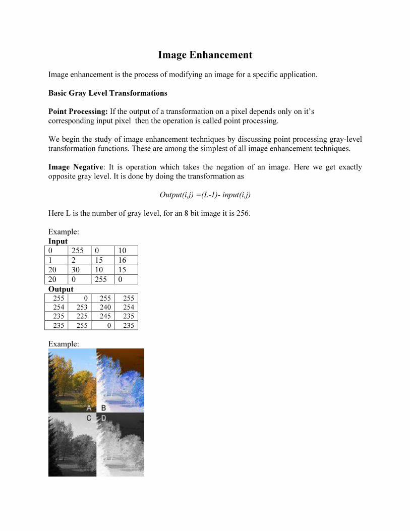
Image Enhancement
Image enhancement is the process of modifying an image for a specific application.
Basic Gray Level Transformations
Point Processing: If the output of a transformation on a pixel depends only on it’s
corresponding input pixel then the operation is called point processing.
We begin the study of image enhancement techniques by discussing point processing gray-level
transformation functions. These are among the simplest of all image enhancement techniques.
Image Negative: It is operation which takes the negation of an image. Here we get exactly
opposite gray level. It is done by doing the transformation as
Output(i,j) =(L-1)- input(i,j)
Here L is the number of gray level, for an 8 bit image it is 256.
Example:
Input
0 255 0 10
1 2 15 16
20 30 10 15
20 0 255 0
Output 255 0 255 255
254 253 240 254
235 225 245 235
235 255 0 235
Example:
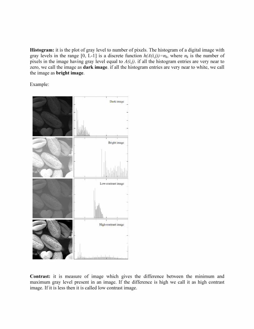
Histogram: it is the plot of gray level to number of pixels. The histogram of a digital image with
gray levels in the range [0, L-1] is a discrete function h(A(i,j))=nk, where nk is the number of
pixels in the image having gray level equal to A(i,j). if all the histogram entries are very near to
zero, we call the image as dark image. if all the histogram entries are very near to white, we call
the image as bright image.
Example:
Contrast: it is measure of image which gives the difference between the minimum and
maximum gray level present in an image. If the difference is high we call it as high contrast
image. If it is less then it is called low contrast image.
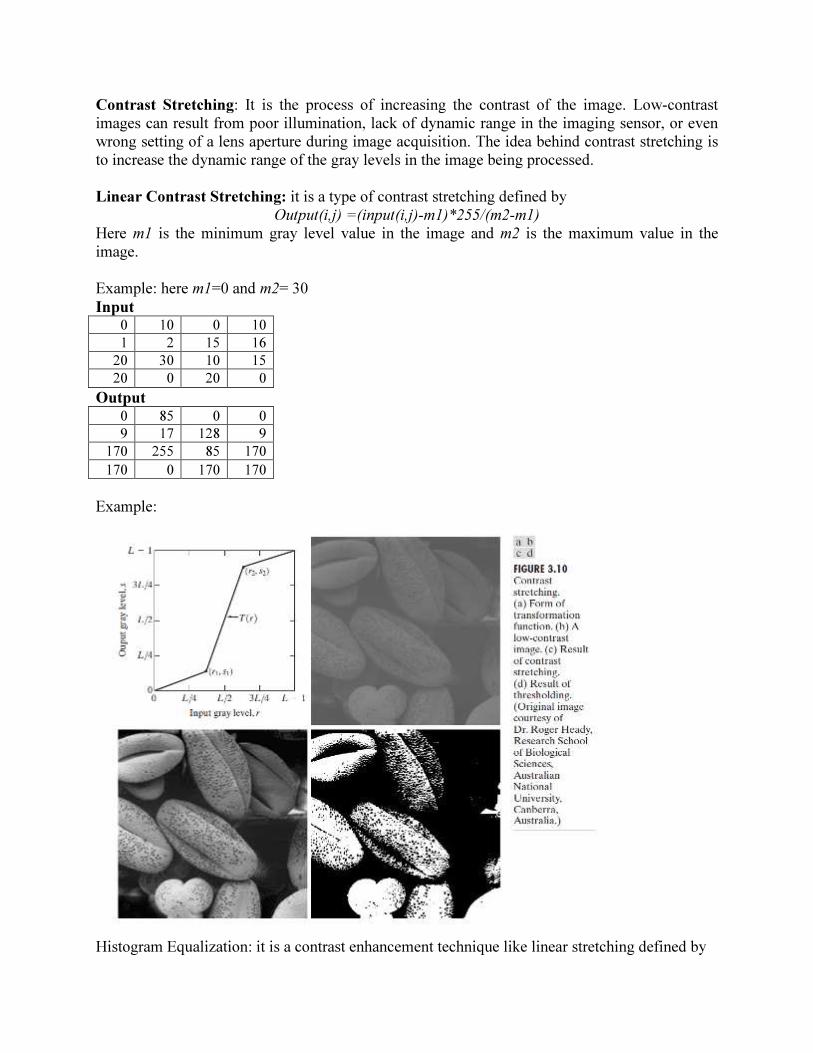
Contrast Stretching: It is the process of increasing the contrast of the image. Low-contrast
images can result from poor illumination, lack of dynamic range in the imaging sensor, or even
wrong setting of a lens aperture during image acquisition. The idea behind contrast stretching is
to increase the dynamic range of the gray levels in the image being processed.
Linear Contrast Stretching: it is a type of contrast stretching defined by
Output(i,j) =(input(i,j)-m1)*255/(m2-m1)
Here m1 is the minimum gray level value in the image and m2 is the maximum value in the
image.
Example: here m1=0 and m2= 30
Input 0 10 0 10 1 2 15 16
20 30 10 15 20 0 20 0
Output
0 85 0 0
9 17 128 9
170 255 85 170
170 0 170 170
Example:
Histogram Equalization: it is a contrast enhancement technique like linear stretching defined by
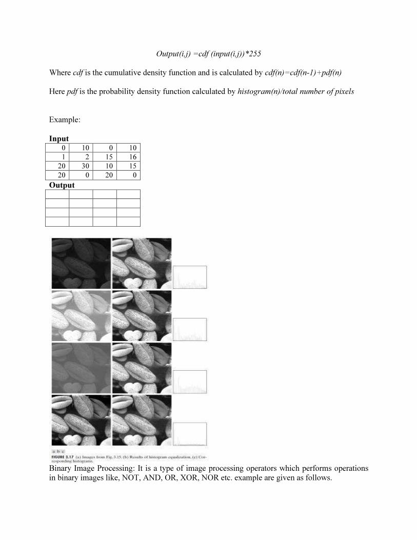
Output(i,j) =cdf (input(i,j))*255
Where cdf is the cumulative density function and is calculated by cdf(n)=cdf(n-1)+pdf(n)
Here pdf is the probability density function calculated by histogram(n)/total number of pixels
Example:
Input 0 10 0 10 1 2 15 16
20 30 10 15 20 0 20 0
Output
Binary Image Processing: It is a type of image processing operators which performs operations
in binary images like, NOT, AND, OR, XOR, NOR etc. example are given as follows.
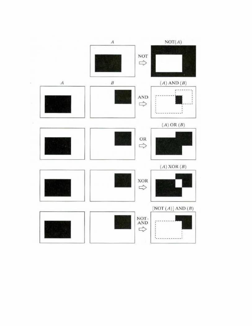
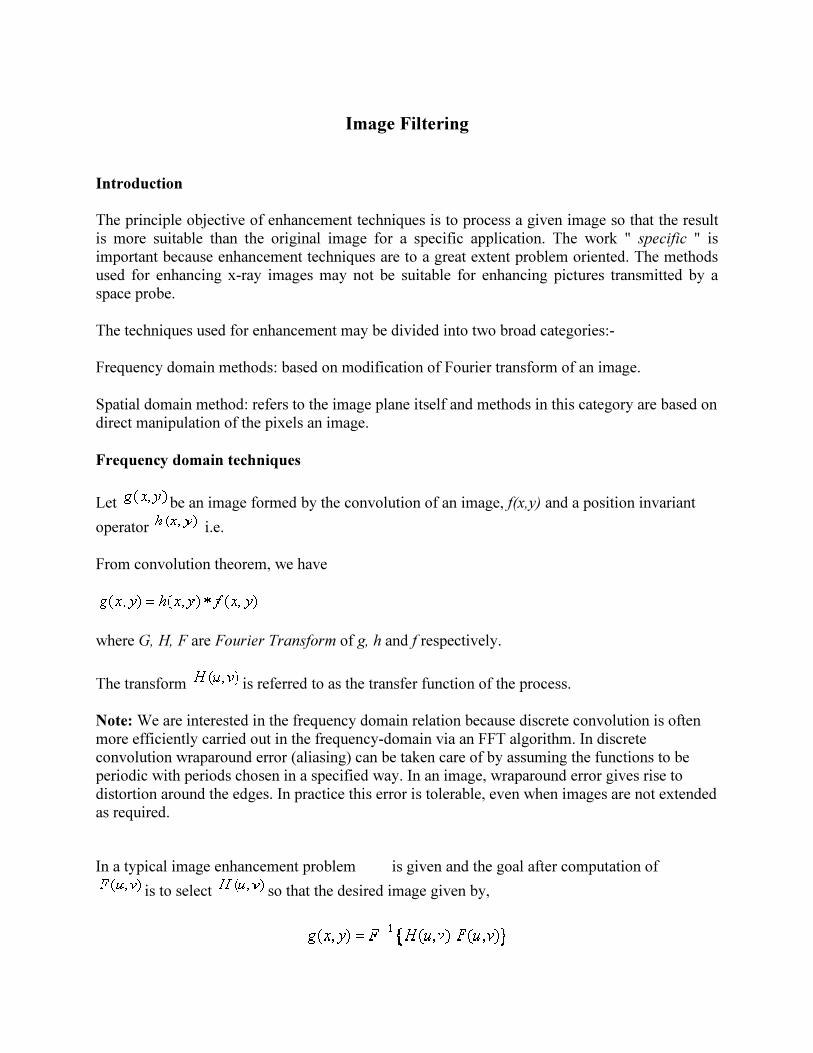
Image Filtering
Introduction
The principle objective of enhancement techniques is to process a given image so that the result
is more suitable than the original image for a specific application. The work " specific " is
important because enhancement techniques are to a great extent problem oriented. The methods
used for enhancing x-ray images may not be suitable for enhancing pictures transmitted by a
space probe.
The techniques used for enhancement may be divided into two broad categories:-
Frequency domain methods: based on modification of Fourier transform of an image.
Spatial domain method: refers to the image plane itself and methods in this category are based on
direct manipulation of the pixels an image.
Frequency domain techniques
Let be an image formed by the convolution of an image, f(x,y) and a position invariant
operator i.e.
From convolution theorem, we have
where G, H, F are Fourier Transform of g, h and f respectively.
The transform is referred to as the transfer function of the process.
Note: We are interested in the frequency domain relation because discrete convolution is often
more efficiently carried out in the frequency-domain via an FFT algorithm. In discrete
convolution wraparound error (aliasing) can be taken care of by assuming the functions to be
periodic with periods chosen in a specified way. In an image, wraparound error gives rise to
distortion around the edges. In practice this error is tolerable, even when images are not extended
as required.
In a typical image enhancement problem is given and the goal after computation of
is to select so that the desired image given by,
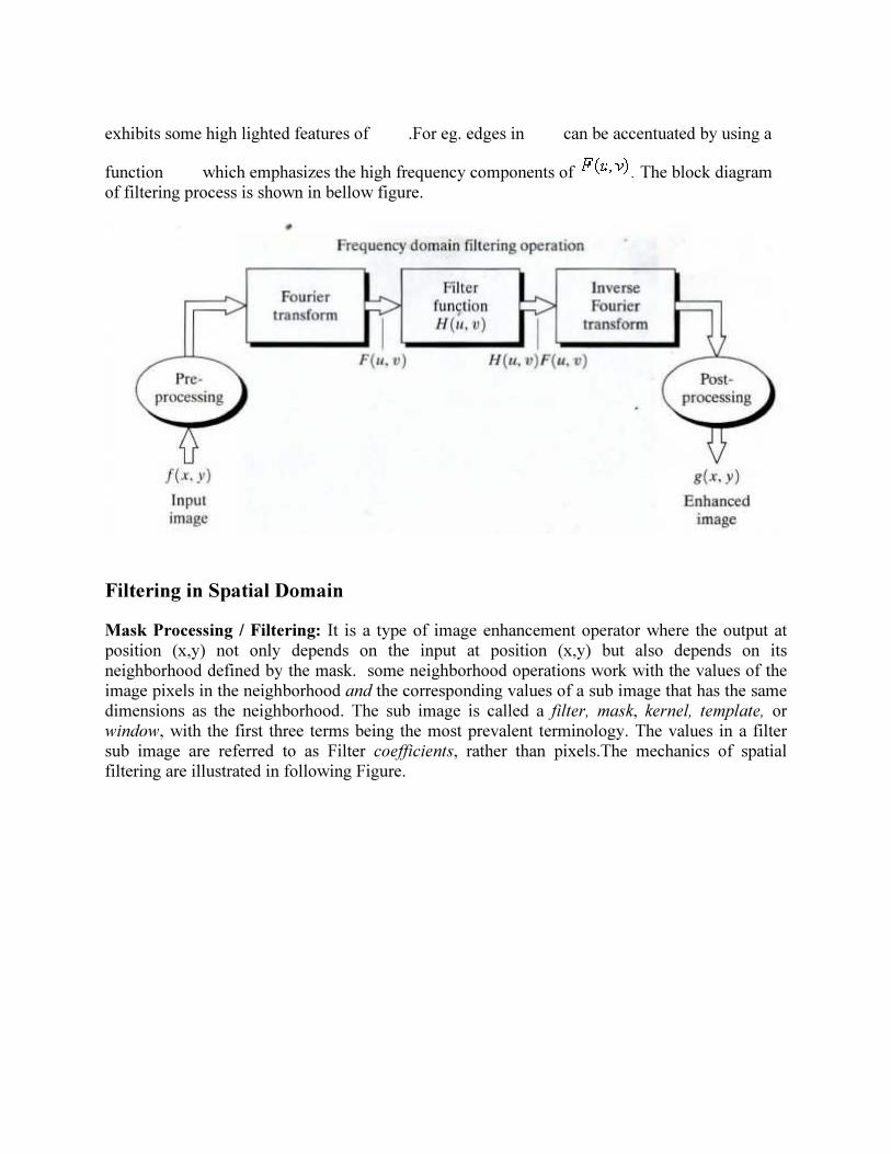
exhibits some high lighted features of .For eg. edges in can be accentuated by using a
function which emphasizes the high frequency components of . The block diagram
of filtering process is shown in bellow figure.
Filtering in Spatial Domain
Mask Processing / Filtering: It is a type of image enhancement operator where the output at
position (x,y) not only depends on the input at position (x,y) but also depends on its
neighborhood defined by the mask. some neighborhood operations work with the values of the
image pixels in the neighborhood and the corresponding values of a sub image that has the same
dimensions as the neighborhood. The sub image is called a filter, mask, kernel, template, or
window, with the first three terms being the most prevalent terminology. The values in a filter
sub image are referred to as Filter coefficients, rather than pixels.The mechanics of spatial
filtering are illustrated in following Figure.
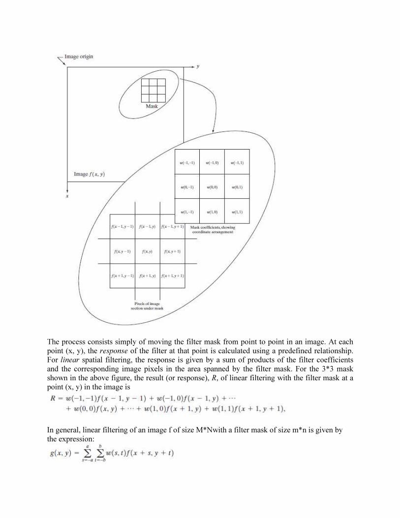
The process consists simply of moving the filter mask from point to point in an image. At each
point (x, y), the response of the filter at that point is calculated using a predefined relationship.
For linear spatial filtering, the response is given by a sum of products of the filter coefficients
and the corresponding image pixels in the area spanned by the filter mask. For the 3*3 mask
shown in the above figure, the result (or response), R, of linear filtering with the filter mask at a
point (x, y) in the image is
In general, linear filtering of an image f of size M*Nwith a filter mask of size m*n is given by
the expression:
where, a=(m-1)/2 and b=(n-1)/2.
Spatial Filters
Spatial filters can be classified by effect into:
1. Smoothing Spatial Filters: also called lowpass filters. They include:
1.1 Averaging linear filters
1.2 Order-statistics nonlinear filters.
2. Sharpening Spatial Filters: also called highpass filters. For example,
the Laplacian linear filter.
Smoothing Spatial Filters are used for blurring and for noise reduction. Blurring is used in
Preprocessing steps to: remove small details from an image prior to (large) object extraction
Bridge small gaps in lines or curves.
Noise reduction can be accomplished by blurring with a linear filter and also by nonlinear
filtering.
Averaging linear filters
The response of averaging filter is simply the average of the pixels contained in the
neighborhood of the filter mask. The output of averaging filters is a smoothed image with
reduced "sharp" transitions in gray levels. Noise and edges consist of sharp transitions in gray
levels. Thus smoothing filters are used for noise reduction; however, they have the undesirable
side effect that they blur edges.
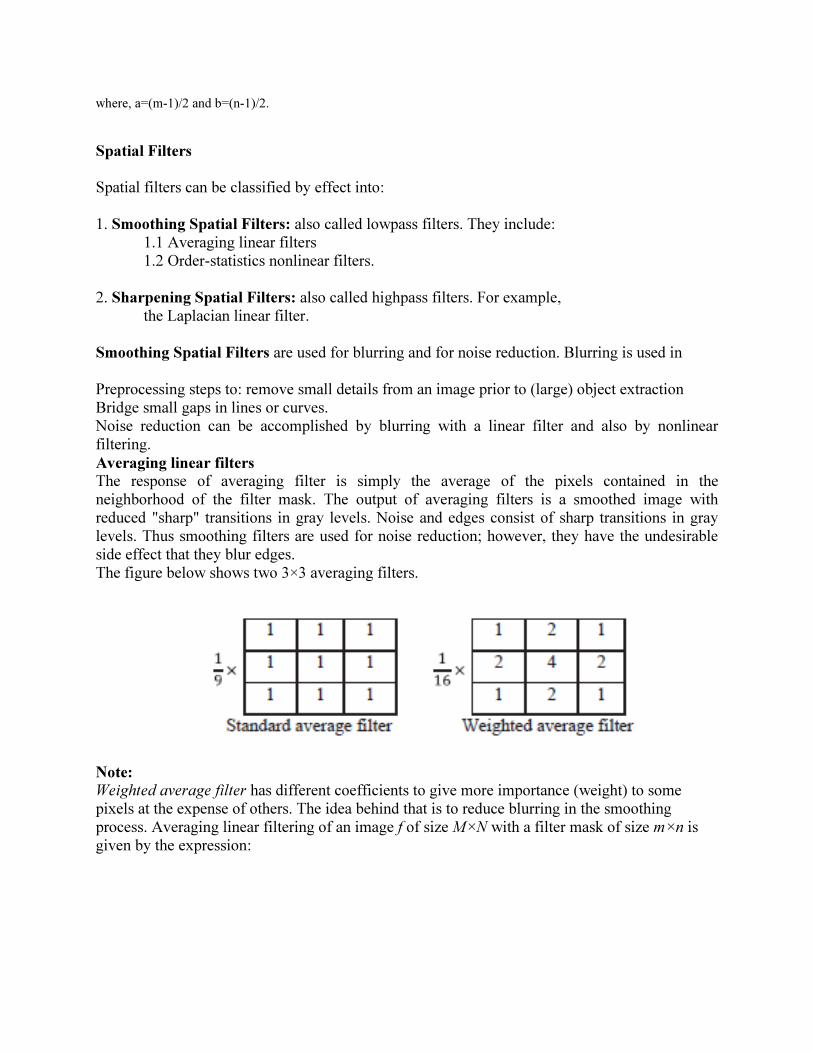
The figure below shows two 3×3 averaging filters.
Note:
Weighted average filter has different coefficients to give more importance (weight) to some
pixels at the expense of others. The idea behind that is to reduce blurring in the smoothing
process. Averaging linear filtering of an image f of size M×N with a filter mask of size m×n is
given by the expression:
To generate a complete filtered image this equation must be applied for x = 0,1, 2,..., M-1 and y
= 0,1, 2,..., N-1.
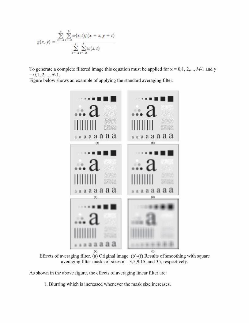
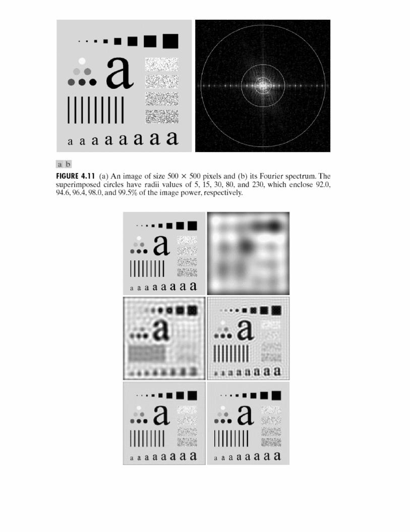
Figure below shows an example of applying the standard averaging filter.
Effects of averaging filter. (a) Original image. (b)-(f) Results of smoothing with square
averaging filter masks of sizes n = 3,5,9,15, and 35, respectively.
As shown in the above figure, the effects of averaging linear filter are:
1. Blurring which is increased whenever the mask size increases.
2. Blending (removing) small objects with the background. The size of the mask
establishes the relative size of the blended objects.
3. Black border because of padding the borders of the original image.
4. Reduced image quality.
Order-statistics filters are nonlinear spatial filters whose response is based on ordering
(ranking) the pixels contained in the neighborhood, and then replacing the value of the center
pixel with the value determined by the ranking result. Examples include Max, Min, and Median
filters.
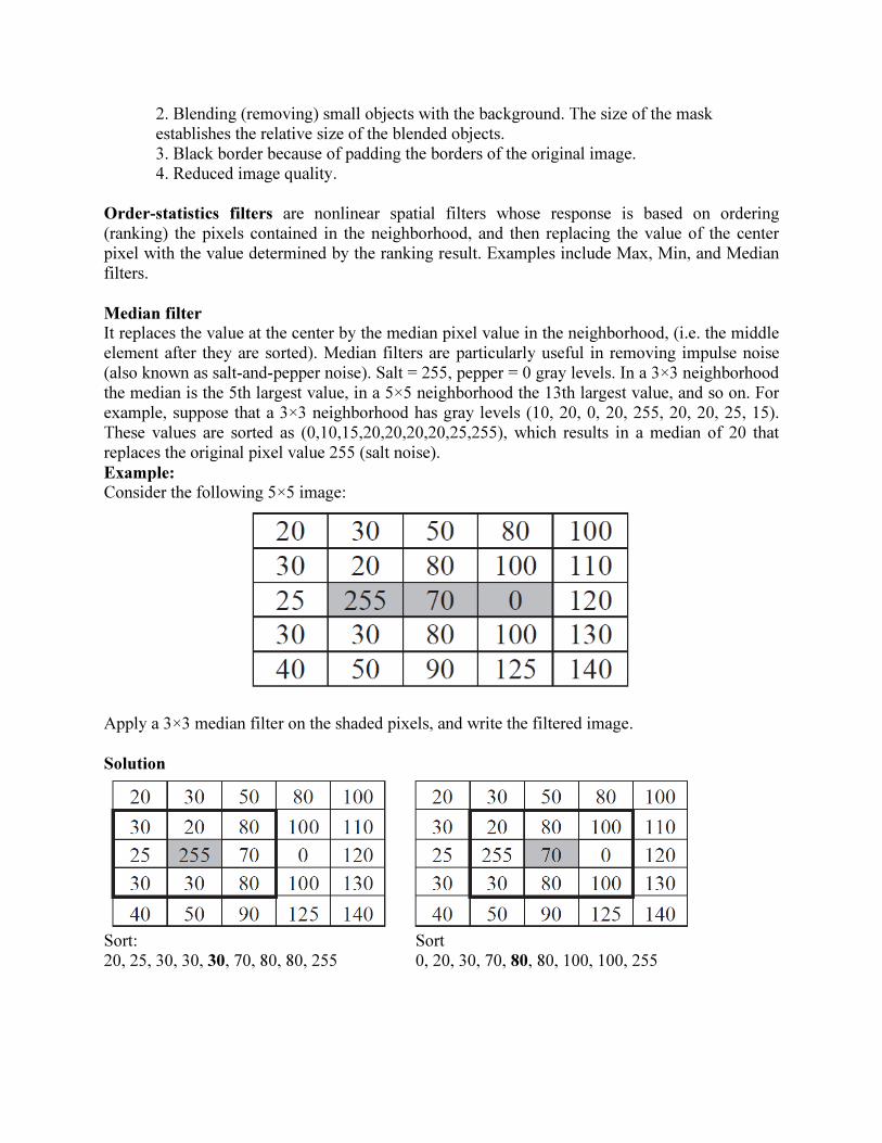
Median filter
It replaces the value at the center by the median pixel value in the neighborhood, (i.e. the middle
element after they are sorted). Median filters are particularly useful in removing impulse noise
(also known as salt-and-pepper noise). Salt = 255, pepper = 0 gray levels. In a 3×3 neighborhood
the median is the 5th largest value, in a 5×5 neighborhood the 13th largest value, and so on. For
example, suppose that a 3×3 neighborhood has gray levels (10, 20, 0, 20, 255, 20, 20, 25, 15).
These values are sorted as (0,10,15,20,20,20,20,25,255), which results in a median of 20 that
replaces the original pixel value 255 (salt noise).
Example:
Consider the following 5×5 image:
Apply a 3×3 median filter on the shaded pixels, and write the filtered image.
Solution
Sort: Sort
20, 25, 30, 30, 30, 70, 80, 80, 255 0, 20, 30, 70, 80, 80, 100, 100, 255
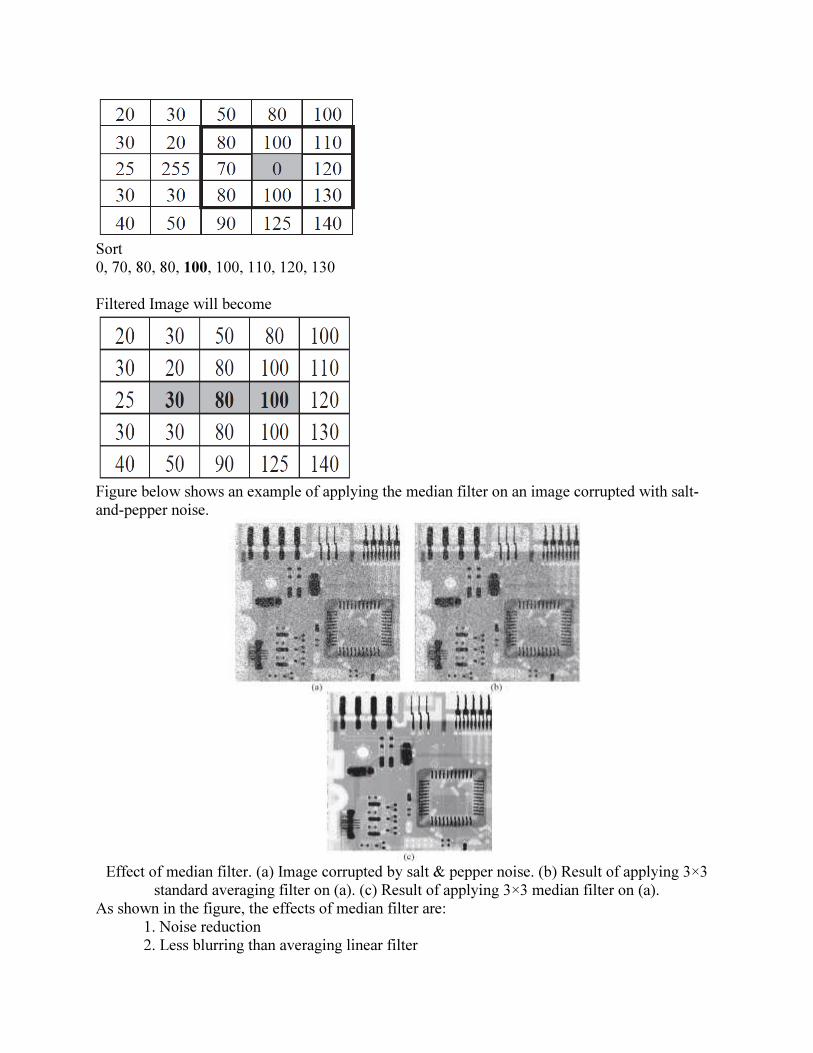
Sort
0, 70, 80, 80, 100, 100, 110, 120, 130
Filtered Image will become
Figure below shows an example of applying the median filter on an image corrupted with salt-
and-pepper noise.
Effect of median filter. (a) Image corrupted by salt & pepper noise. (b) Result of applying 3×3
standard averaging filter on (a). (c) Result of applying 3×3 median filter on (a).
As shown in the figure, the effects of median filter are:
1. Noise reduction
2. Less blurring than averaging linear filter
Sharpening Spatial Filters
Sharpening aims to highlight fine details (e.g. edges) in an image, or enhance detail that has been
blurred through errors or imperfect capturing devices. Image blurring can be achieved using
averaging filters, and hence sharpening can be achieved by operators that invert averaging
operators. In mathematics, averaging is equivalent to the concept of integration, and
differentiation inverts integration. Thus, sharpening spatial filters can be represented by partial
derivatives.
Partial derivatives of digital functions
The first order partial derivatives of the digital image f(x,y) are:
The first derivative must be:
1) zero along flat segments (i.e. constant gray values).
2) non-zero at the outset of gray level step or ramp (edges or noise)
3) non-zero along segments of continuing changes (i.e. ramps).
The second order partial derivatives of the digital image f(x,y) are:
The second derivative must be:
1) zero along flat segments.
2) nonzero at the outset and end of a gray-level step or ramp;
3) zero along ramps
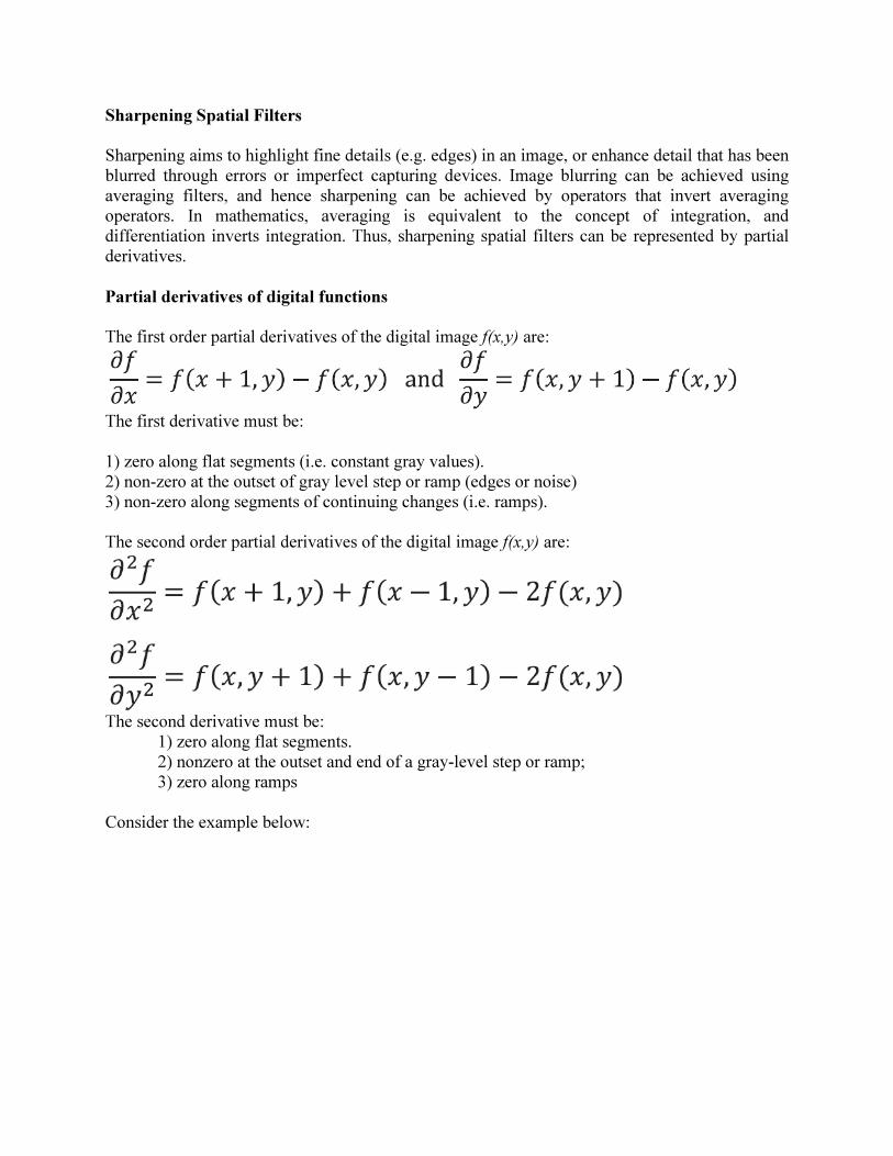
Consider the example below:
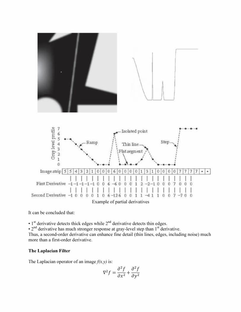
Example of partial derivatives
It can be concluded that:
• 1st derivative detects thick edges while 2
nd derivative detects thin edges.
• 2nd derivative has much stronger response at gray-level step than 1
st derivative.
Thus, a second-order derivative can enhance fine detail (thin lines, edges, including noise) much
more than a first-order derivative.
The Laplacian Filter
The Laplacian operator of an image f(x,y) is:
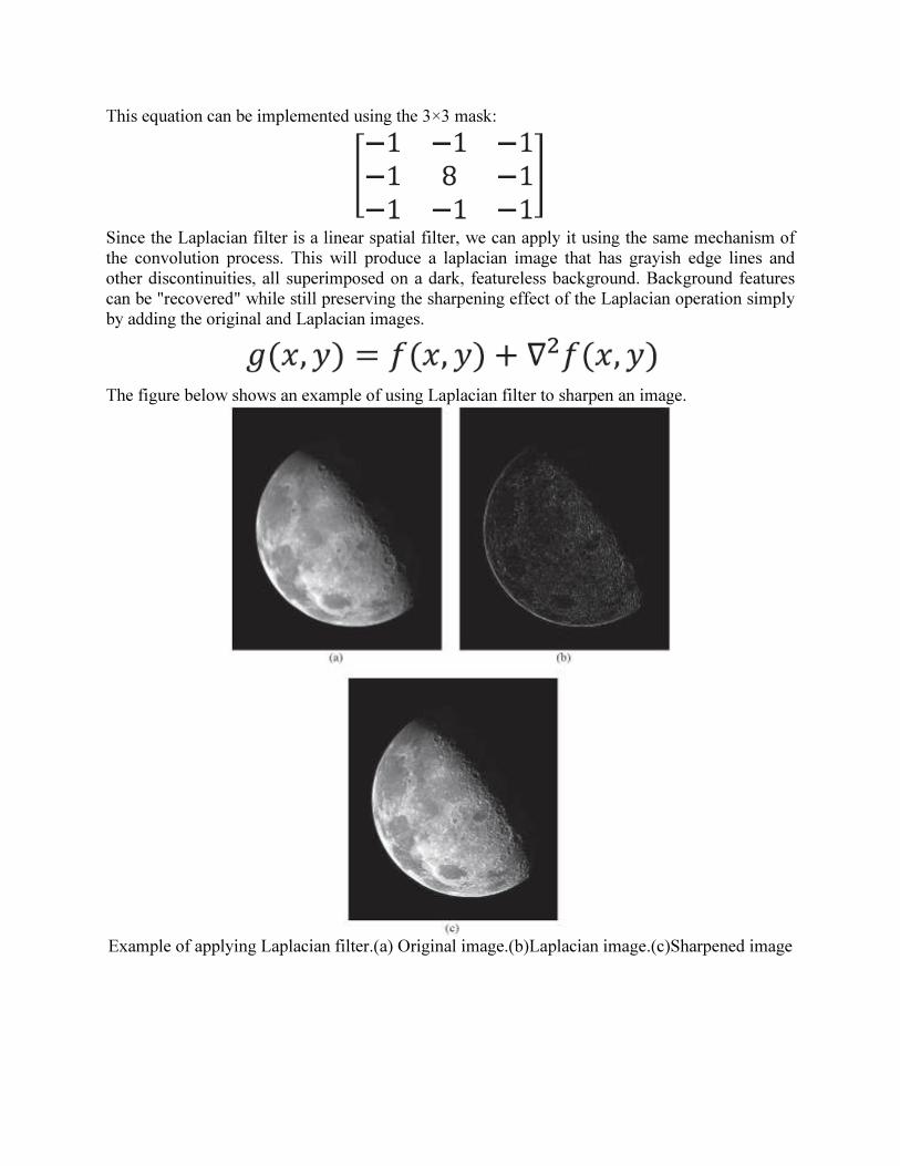
This equation can be implemented using the 3×3 mask:
Since the Laplacian filter is a linear spatial filter, we can apply it using the same mechanism of
the convolution process. This will produce a laplacian image that has grayish edge lines and
other discontinuities, all superimposed on a dark, featureless background. Background features
can be "recovered" while still preserving the sharpening effect of the Laplacian operation simply
by adding the original and Laplacian images.
The figure below shows an example of using Laplacian filter to sharpen an image.
Example of applying Laplacian filter.(a) Original image.(b)Laplacian image.(c)Sharpened image
Enhancement in Frequency Domain
• The frequency content of an image refers to the rate at which the gray levels change in the
image.
• Rapidly changing brightness values correspond to high frequency terms, slowly changing
brightness values correspond to low frequency terms.
• The Fourier transform is a mathematical tool that analyses a signal (e.g. images) into its
spectral components depending on its wavelength (i.e. frequency content).
2D Discrete Fourier Transform
The DFT of a digitized function f(x,y) (i.e. an image) is defined as:
The domain of u and v values u = 0, 1, ..., M-1, v = 0,1,…, N-1 is called the frequency domain of
f(x,y).
The magnitude of , is called the Fourier
spectrum of the transform.
The phase angle (phase spectrum) of the transform is:
Note that, F(0,0) = the average value of f(x,y) and is referred to as the dc component of the
spectrum. It is a common practice to multiply the image f(x,y) by (-1)x+y. In this case, the DFT of
(f(x,y)(-1)x+y)
has its origin located at the centre of the image, i.e. at (u,v) = (M/2,N/2).
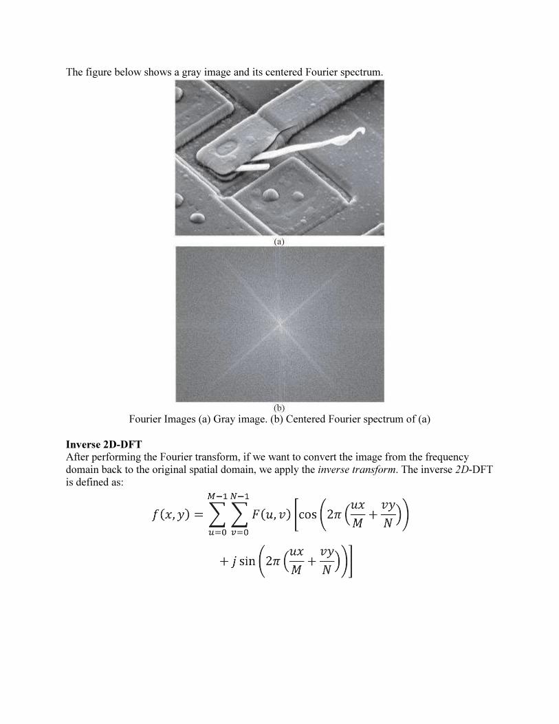
The figure below shows a gray image and its centered Fourier spectrum.
Fourier Images (a) Gray image. (b) Centered Fourier spectrum of (a)
Inverse 2D-DFT
After performing the Fourier transform, if we want to convert the image from the frequency
domain back to the original spatial domain, we apply the inverse transform. The inverse 2D-DFT
is defined as:
Frequency domain vs. Spatial domain
Frequency domain Spatial domain
1. is resulted from Fourier transform values of the Fourier transform and its
frequency variables (u,v). is resulted from
sampling and quantization
2. refers to the space defined by i.e. the total
number of pixels composing an image, each
has spatial coordinates (x,y)
refers to the image plane itself,
3. has complex quantities has integer quantities
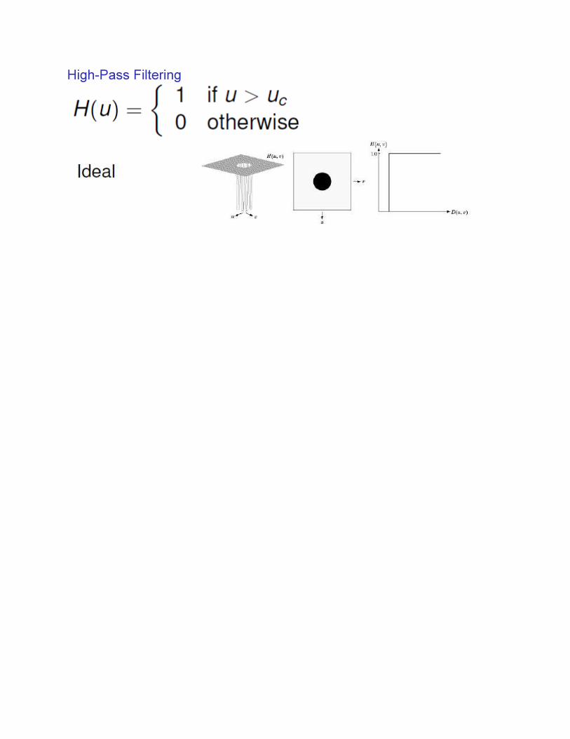
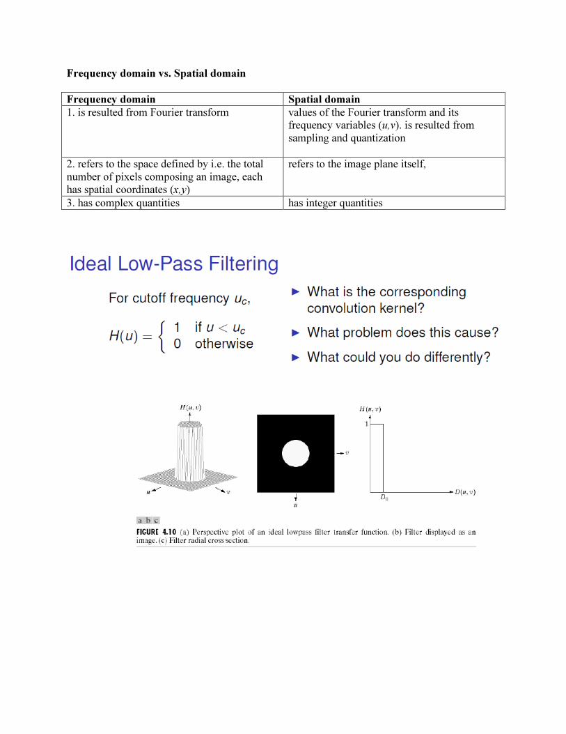
High-Pass Filtering
Recommended