1
VALUE AT RISK AND CONDITIONAL VALUE AT RISK
Robert Powell
School of Accounting, Finance & Economics
Edith Cowan University
Phone: 94022801
Email: [email protected]
Abstract: Value at Risk (VaR) is an important issue for banks since its adoption as a primary risk metric
in the Basel Accords. Value at Risk (VaR) and Conditional VaR (CVaR) in Australia is
examined from an industry perspective using a set of Australian industries. A variety of
metrics is used, including diversified and undiversified VaR, as well as parametric and
nonparametric CVaR methods. There is found to be no significant difference between these
metrics in ranking industry risk, with the highest relative industry risk in the Technology
Sectors, and lowest risk in the Finance and Utilities Sectors.
2
Preface
Title of Thesis: Industry Value at Risk in Australia
Supervisor: Professor David Allen
Two key risks faced by banks are market risk and credit risk. Value at risk (VaR) measures
the maximum expected market or credit loss over a given time period at a given level of
confidence. My thesis compares risk across Australian industries using a variety of market
and credit metrics. In addition, I examine extreme Conditional Value at Risk (CVaR), which
measures extreme risk. The thesis identifies limitations with existing market and credit VaR
and CVaR models, and develops new modelling techniques to overcome these limitations.
Finally, the study develops a set of Australian sector risk indices, and develops a new model
(called iTransition) which incorporates both credit and market elements.
The thesis is structured as followed:
Chapter 1: Introduction
Chapter 2: Literature survey on VaR and CVaR modelling techniques for market and
credit risk
Chapter 3: Methodology (techniques used by my study for measuring market and credit
Industry VaR and CVaR in Australia, including development of new
techniques)
Chapter 4: Results of the industry modelling
Chapter 5: Development of sector indices and iTransition model
Chapter 6: Conclusions and recommendations for further research
This paper summarises the market risk aspects of my thesis.
3
1. Introduction
VaR models have gained increasing momentum since the VaR concept was first
introduced by JP Morgan in 1994. This momentum was spurred by amendments to the Basel
Accord in 1996 which required Banks to set aside capital for meeting Market Risk. Market
risk arises from factors that affect the whole market. This paper focuses on equities and
compares relative VaR and CVaR across 25 Australian industries, based on equity price
movements using a parametric distribution, which is the most widely used approach among
Banks. VaR has become the recognised standard approach for market risk measurement. VaR
calculates maximum expected losses over a given time period at a given tolerance level.
In addition to VaR, this paper examines extreme industry risk using (conditional)
CVaR. CVaR considers extreme events, based on losses exceeding VaR. Whilst there have
been a wide range of VaR studies in USA and European markets, the vast majority have
centred around individual asset or overall portfolio VaR as opposed to adopting a sectoral
approach. There is very little study of industry risk using VaR approaches in the Australian
market, and even less on CVaR. Indeed, very little research has been undertaken on the uses
and applications of VaR or related metrics at all in Australia. (A search of APRA’s website at
http://www.apra.gov.au/RePEc/Home.cfm?FormStatus=Sent&TargetSeries=Working%20Pap
ers:RePEc:apr:aprewp revealed Sy (2006), Engel and Gizycki (1999) and Gizycki and
Hereford (1999) as being the only papers considering aspects of VaR).
This paper aims to provide a greater understanding of the VaR and CVaR modelling
approaches, as well as industry risk, in an Australian context. Industry market VaR is
measured for each industry in Australia based on the variance-covariance parametric model,
using both diversified and undiversified approaches. CVaR is measured using both parametric
and nonparametric methodology. The study also compares VaR and CVaR changes between
industries over time.
This comprehensive exploration and application of these various VaR metrics should
indicate whether the measures are robust and consistent over time and across industry sectors.
The paper is divided into eight sections: section two provides a brief review of the Australian
equities market whilst sections three and four review the concepts and calculation methods of
VaR and CVaR. Section five reviews the data used and the research method, and the analysis
is presented in section six. Section seven presents the results from the viewpoint of industrial
sectors and section eight concludes.

4
2. The Australian Market
There has been significant recent growth in the Australian Equities Market. In 1992,
the Australian domestic market capitalisation was $198 billion, and this has since grown to
$1.4 trillion. Appendix 1 shows the sector and sub sector classifications used by the
Australian Stock Exchange (ASX). These sectors are based on the Global Industry
Classification Standard (GICS) which is a joint Standard & Poor’s / Morgan Stanley Capital
International Product aimed at standardising global industry classifications.
The S&P/ASX 200 is recognised as the investable benchmark for the Australian
equity market and comprises 200 stocks selected by the S&P Australian Index Committee and
represents approximately 90% of the total market capitalisation of the Australian Market
(2006). The All Ordinaries index (All Ords) is considered to be Australia’s market indicator,
representing the 500 largest companies listed on the stock exchange (Standard & Poor's,
2006), and is the index used in this paper. Appendix 2 provides a breakdown of the market
capitalisation of All Ords companies.
3. Background to Value at Risk and Conditional Value at Risk
The use of VaR has become all-pervasive in a relatively short period of time despite
its conceptual and practical shortcomings. VaR received its first broad recommendation in the
Group of Thirty Report (1993). Subsequently its use and recognition have increased
dramatically, particularly when the Basel Committee on Banking Supervision adopted the use
of VaR models, contingent upon certain qualitative and quantitative standards. VaR has
subsequently become one of the most important and widely used measures of risk. As a risk-
management technique VaR describes the loss that can occur over a given period, at a given
confidence level, due to exposure to market risk. The appealing simplicity of the VaR concept
has lead to its adoption as a standard risk measure for financial entities involved in large scale
trading operations, but also retail banks, insurance companies, institutional investors, and non-
financial enterprises. Its use is encouraged by the Bank for International Settlements, the
American Federal Reserve Bank and the Securities and Exchange Commission.
5
The groundbreaking Basel Capital Accord, originally signed by the Group of Ten
(G10) countries in 1988, but since largely adopted by over 100 countries, requires Authorised
Deposit-taking Institutions (ADI’s) to hold sufficient capital to provide a cushion against
unexpected losses. Value-at-Risk (VaR) is a procedure designed to forecast the maximum
expected loss over a target horizon, given a (statistical) confidence limit. Initially, the Basel
Accord stipulated a standardized approach which all institutions were required to adopt in
calculating their VaR thresholds. This approach suffered from several deficiencies, the most
notable of which were its conservatism (or lost opportunities) and its failure to reward
institutions with superior risk management expertise.
Following much industry criticism, the Basel Accord was amended in April 1995 to
allow institutions to use internal models to determine their VaR and the required capital
charges. However, institutions wishing to use their own models are required to have the
internal models evaluated by the regulators using the back-testing procedure. The Basel
Accord (BA) was adopted by the Australian government in 1988, with the Australian
Prudential Regulatory Authority (APRA) as the national regulator of financial markets.
According to APRA, Australia is now fully compliant with 11 BA principles, largely
compliant with 12, and materially non-compliant with 2. Importantly, Australia is compliant
with Principle 12, which states that:
“Banking supervisors must be satisfied that banks have in place systems that
accurately measure, monitor and adequately control market risk; supervisors should have the
powers to impose specific limits and/or a specific capital charge on market risk exposures, if
warranted.”
A description of the various methodologies for the modelling of VaR can be seen at
http://www.gloriamundi.org/ . The predominant approaches to calculating VaR rely on a
linear approximation of the portfolio risks and assume a joint normal (or log-normal)
distribution of the underlying market processes. There is a comprehensive survey of the
concept by Duffie and Pan (1997), and discussions in Jorion (1996), Pritsker (1997)
RiskMetricsTM (1996) , Beder (1995), and Stambaugh (1996).
Despite its universal adoption and promotion by the regulatory authorities and its
embrace by the financial services industry there are a number of theoretical and practical
difficulties associated with the use of VaR as a risk metric. A standard procedure, in terms of
the practical implementation of VaR metrics, if the portfolio of concern contains non-linear
instruments such as options, is to make recourse to historical or Monte-Carlo simulation based
6
tools. See the discussions in Bucay and Rosen (1999), Jorion (1996), Mauser and Rosen
(1999), Pritsker (1997), RiskMetricsTM (1996), Beder (1995), and Stambaugh (1996). The
optimisation problems associated with calculating VaR are discussed in papers by Litterman
(1997a) and (1997b), Kast et al (1998), and Lucas and Klaussen (1998).
Nevertheless, despite its popularity, VaR has certain undesirable mathematical
properties; such as lack of sub-additivity and convexity; see the discussion in Arztner et al
(1997) and (1999). In the case of the standard normal distribution VaR is proportional to the
standard deviation and is coherent when based on this distribution but not in other
circumstances. The VaR resulting from the combination of two portfolios can be greater than
the sum of the risks of the individual portfolios. A further complication is associated with the
fact that VaR is difficult to optimize when calculated from scenarios. It can be difficult to
resolve as a function of a portfolio position and can exhibit multiple local extrema, which
makes it problematic to determine the optimal mix of positions and the VaR of a particular
mix. See the discussion of this in Mckay and Keefer (1996) and Mauser and Rosen (1999).
This paper features the exploration and application of an alternative to VaR: CVaR –
Conditional-Value-at-Risk. Pflug (2000) proved that CVaR is a coherent risk measure with a
number of desirable properties such as convexity and monotonicity w.r.t stochastic dominance
of order 1, amongst other desirable characteristics. Furthermore, VaR gives no indication on
the extent of the losses that might be encountered beyond the threshold amount suggested by
the measure. By contrast CVaR does quantify the losses that might be encountered in the tail
of the distribution. This is because a portfolio’s CVaR is the loss one expects to suffer, given
that the loss is equal to or larger than its VaR. A number of recent papers apply CVaR to
portfolio optimization problems; see for example Rockafeller and Uryasev (1999) and (2002),
Andersson et.al (2000), Alexander, Coleman & Li (2003), Alexander and Baptista (2003) and
Rockafellar et al (2006). However, there has been no prior use or application of CVaR in an
Australian setting and its use, properties and applications are still in the early stages of their
development.
4. Calculating Value at Risk and Conditional Value at Risk
VaR calculates maximum expected losses over a given time period at a given
tolerance level. There are 3 methods of calculating VaR. The Variance-Covariance method
7
estimates VaR on assumption of a normal distribution. The historical method groups historical
losses in categories from best to worst and calculates VaR on the assumption of history
repeating itself. The Monte Carlo method simulates multiple random scenarios.
The Variance-Covariance approach is the most widely used approach, and is the
method we use in this study. To obtain VaR for a single asset X, the mean and standard
deviation are calculated. Given the normal distribution assumption, we know where the worst
1% and 5% lie on the curve. VaR at 95% confidence level = 1.645 x ơx and at 99% confidence
level = 2.330 x ơx. When calculating VaR, it is usual practice to not use actual asset figures,
but the logarithm of the ratio of price relatives, which is the method used by RiskMetricsTM
(1996). This is obtained by using the following calculation:
⎟⎟⎠
⎞⎜⎜⎝
⎛
−1
lnt
t
PP
(4-1)
i.e. the logarithm of the ratio between today’s price and the previous price. The
standard deviation is annualised by multiplying it by the square root of the number of trading
days per annum (usually taken to be 250).
When additional assets are introduced into the portfolio, we need to account for
correlations between the assets. Portfolio variance is calculated as follows, with w being the
relative weighting of the assets:
yxyxyxyyxxport wwwwV ρσσσσ 22222 ++= (4-2)
When dealing with multiple assets, variance-covariance matrix multiplication is used.
The portfolio standard deviation is the square root of the variance multiplied by the square
root of 250.
CVaR is the mean value of the losses beyond VaR. For instance, if we are measuring
VaR at a 95% confidence level, CVaR is the average of the 5% worst losses. CVaR can be
calculated using the actual 5% worst losses (nonparametric), or using a normal distribution
(parametric) approach, as follows (Huang, 2000):
8
σπα
α
α 2
)2
exp(2q
CVaR−
= (4-3)
Where qα is the tail 100α percentile of a standard normal distribution (e.g. 1.645 as
obtained from standard distribution tables for 95% confidence).
5. Data and Research Methodology
5.1. Data
We use the All Ords and obtain daily share prices for the last 15 years (which is the
maximum available) from Datastream. For market VaR, Basel requires 250 days data. This is
only 1 year, and we are more concerned with a longer term perspective, spanning different
economic conditions. It should be noted at this stage that this paper is a summary of the
market VaR section of a wider study which also includes Credit VaR. This wider study
compares VaR between credit models and market models to ascertain whether there is a
correlation between the industries that are risky from a credit perspective and those that are
risky from a market perspective. The study follows the Basel requirement for 7 years data for
the advanced credit approach (Bank for International Settlements, 2004, p.98). For
comparison purposes, and to meet our requirement for longer market perspectives, we also
use 7 year windows for calculating market VaR. This allows 9 years of comparative data (the
first tranche being years 1-7, second tranche years 2-8, and so on until the 9th tranche which
represents the 7 years from 9 – 15 of our data sample). We recognise that the longer sample
may have different results to a shorter sample, and so we also do an historical comparison
using 250 day windows. Industry codes are obtained from the ASX website and Market
Capitalisation (for weighting of market VaR company data) is obtained from Datastream.
9
5.2. Data Limitations & Considerations
The data poses some limitations & considerations, such as the fact that the industry
classifications used by Datastream are different from those used by the ASX, and that some
industries have very few entities from which to make meaningful conclusions. The balance of
this section outlines some of these issues and how we overcome them.
5.2.1. Sector accuracy, classification and size
Datastream uses the UK FTSE industry classifications. To ensure accuracy of
classification, and to align with what is actually used on the ASX and by Moody’s and
Standard & Poor’s, all companies in this study have been re-classified to GICS. This is done
by obtaining individual GICS codes for each entity from the ASX website. To ensure a
meaningful quantity of data, Sectors with less than 5 companies, and companies with less than
12 months data have been excluded. The remaining companies represent 93% of those in the
All Ords Index by both number and market capitalisation. As the All Ords represent more
than 90% of the value of listed Australian companies, we consider 5 entities to be sufficient to
provide meaningful conclusions.
5.2.2. Survivorship bias
This occurs when an index only includes current surviving companies and excludes
failed entities (Brailsford & Heaney, 1998). This may cause a favourable bias in the results.
An index such as the All Ords (and all other indices on the ASX) will not include failed
companies as these would have been delisted. We are not be able to include all failed
companies over the 15 years as the historical data for all of these is not available on
Datastream. We were however able to obtain Datastream data for companies placed in
administration or receivership and delisted over the past 3 years. This amounts to 11
companies, spanning 7 industries. To test for the impact of survivorship bias we ran our
model with these companies included in our first rolling window and compared the industry
VaR rankings including failed companies to the results excluding failed companies, testing for
significance using the Spearman Rank Correlation Test (refer Section 5.5). Changes were

10
found to be not significant at the 95% level and we therefore consider survivorship bias not to
have a significant impact on our study.
5.2.3. Thin trading
This problem occurs when infrequently traded companies are included in a time series
analysis. Brailsford & Heaney (1998, p.p. 239-244) describe the effect as being most
prominent in using daily share price data, but can also exist when using weekly or monthly
data. Liquid (highly traded) assets are continually re-pricing based on market information.
When thinly traded asset prices do change, they incorporate all the market information since
the last trade.
This study uses daily price data as less frequent data does not capture the intervening
volatility. A share could start and finish the week on the same price, but have experienced
several up and down daily movements. In particular, it is important for the CVaR measure to
incorporate all extreme price movements. This does give rise to potential thin trading
problems. This can be reduced by avoiding thinly traded assets. In our case we are using the
All Ords index which consists of the top 500 companies on the ASX, thus avoiding the most
thinly traded assets. We further account for thin trading by applying an adjustment factor as
proposed by Miller, Muthuswamy, and Whaley (1994) who suggest that a Moving Average
model reflecting the number of non-trading days should be used to adjust returns. Due to
difficulty in identifying non trading days, the approach shows that this is equivalent to
estimating an AR (1) model from which the required adjustment can be determined. Their
model involves the following regression equation:
ttt RaaR ε++= −121 (5-1)
The residual is then used to estimate the adjusted return as follows:
)1( 2aR tadj
t −=
ε (5-2)
Where adjtR = the return at time t with the thin trading adjustment.
11
5.3. VaR Calculation
We calculate VaR using the methodology described in Section 4. We begin by
calculating the standard deviation of the logarithm of the daily price relatives. Weightings are
calculated for each company according to market capitalisation. Undiversified VaR is
obtained by multiplying the weighted undiversified standard deviation by 1.645 (as obtained
from standard normal distribution tables for 95% confidence level).
Diversified VaR is obtained through construction of a weighted variance-covariance
matrix for each rolling 7 year period, and multiplying the portfolio standard deviation by
1.645. Both undiversified VaR and diversified VaR are annualised by multiplying by the
square root of 250.
5.4. CVaR calculation
We use a parametric approach to calculate VaR, therefore intuitively it makes sense to
use this approach for CVaR. However this approach has some limitations. It will yield a
ranking spread for CVaR that is the same as VaR, which may not highlight the extreme
returns. We therefore use both parametric and nonparametric approaches.
We use equation 4.3 to calculate parametric CVaR. As we have calculated VaR based
on a 95% confidence level, CVaR is based on the worst 5% of losses. Nonparametric CVaR is
calculated as the weighted average of returns beyond VaR.
5.5. Testing for significance
Hypotheses were formulated for the objectives outlined in Section 1. We used
nonparametric testing, as this is particularly suitable for testing ranking and for smaller data
samples (we have 25 industries and 9 time periods). The Pearson Rank Correlation Test to
was used test for ranking association between diversified and undiversified VaR, VaR and
CVaR, parametric and nonparametric CVaR. The Kruksal-Wallis Test was used to test for
12
ranking association over time. The details of these testing methods is beyond the scope of this
paper but can be found in statistical textbooks such as Siegel & Castellan (1988) and Lee, Lee
& Lee (2000). Suffice it to say that each test compares the rankings and arrives at a test
statistic (t for Spearman Rank Correlation, and K for Kruksal-Wallis) which is compared to a
critical value for the level of significance being tested (in our case 95%).
13
6. Results
6.1. Overall Summary
Table 6-1 Results Summary
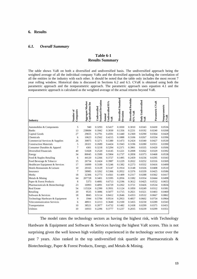
The table shows VaR on both a diversified and undiversified basis. The undiversified approach being the weighted average of all the individual company VaRs and the diversified approach including the correlation of all the entities in the industry with each other. It should be noted that the table only includes the most recent 7 year rolling window. Historical data is discussed in Sections 6.2 and 6.5. CVaR is obtained using both the parametric approach and the nonparametric approach. The parametric approach uses equation 4.1 and the nonparametric approach is calculated as the weighted average of the actual returns beyond VaR.
Industry Num
ber
of
Com
pani
es
Agg
rega
te M
arke
t C
apita
lisat
ion
$m
Und
iver
sifie
d St
anda
rd D
evia
tion
Ann
ual
Und
iver
sifie
d 95
%
VaR
Div
ersi
fied
Stan
dard
D
evia
tion
Div
ersi
fied
Port
folio
95
% V
aR
Dai
ly U
ndiv
ersi
fied
VaR
Par
amet
ric
CV
aR
Non
para
met
ric
CV
aR
Automobiles & Components 5 940 0.3293 0.5417 0.1830 0.3010 0.0343 0.0430 0.0536Banks 13 238684 0.1842 0.3030 0.1356 0.2231 0.0192 0.0240 0.0268Capital Goods 27 29655 0.2791 0.4591 0.1440 0.2369 0.0290 0.0364 0.0428Chemicals 6 10623 0.2562 0.4215 0.1888 0.3106 0.0267 0.0334 0.0396Commercial Services & Supplies 26 30875 0.3271 0.5380 0.1473 0.2424 0.0340 0.0427 0.0530Construction Materials 5 26321 0.2689 0.4424 0.1943 0.3196 0.0280 0.0351 0.0390Consumer Durables & Apparel 7 4301 0.3218 0.5294 0.2371 0.3901 0.0335 0.0420 0.0506Diversified Financials 40 51828 0.2520 0.4145 0.1221 0.2008 0.0262 0.0329 0.0392Energy 34 80045 0.3589 0.5904 0.1737 0.2858 0.0373 0.0468 0.0538Food & Staples Retailing 6 44120 0.2266 0.3727 0.1495 0.2459 0.0236 0.0295 0.0343Food Beverage & Tobacco 15 26734 0.2424 0.3987 0.1229 0.2022 0.0252 0.0316 0.0369Healthcare Equipment & Services 17 16099 0.3189 0.5246 0.1382 0.2273 0.0332 0.0416 0.0499Hotels Restaurants & Leisure 10 20165 0.3129 0.5147 0.1914 0.3148 0.0326 0.0408 0.0510Insurance 7 58985 0.3262 0.5366 0.2052 0.3376 0.0339 0.0425 0.0586Media 18 32306 0.2773 0.4561 0.1409 0.2317 0.0288 0.0362 0.0417Metals & Mining 64 207728 0.3401 0.5595 0.2056 0.3382 0.0354 0.0444 0.0498Paper & Forest Products 8 5373 0.4081 0.6713 0.2196 0.3612 0.0425 0.0532 0.0653Pharmaceuticals & Biotechnology 23 16993 0.4091 0.6729 0.2262 0.3721 0.0426 0.0534 0.0656Real Estate 54 115324 0.2390 0.3931 0.1124 0.1850 0.0249 0.0312 0.0381Retailing 20 9535 0.3086 0.5077 0.1715 0.2821 0.0321 0.0403 0.0469Software & Services 18 8845 0.5114 0.8412 0.2646 0.4353 0.0532 0.0667 0.0862Technology Hardware & Equipment 9 1944 0.5784 0.9514 0.2953 0.4857 0.0602 0.0754 0.0964Telecommunication Services 6 48911 0.2213 0.3640 0.2100 0.3455 0.0230 0.0289 0.0343Transportation 10 38521 0.2877 0.4732 0.1482 0.2438 0.0299 0.0375 0.0451Utilities 10 16933 0.2296 0.3777 0.1237 0.2035 0.0239 0.0299 0.0351
The model rates the technology sectors as having the highest risk, with Technology
Hardware & Equipment and Software & Services having the highest VaR scores. This is not
surprising given the well known high volatility experienced in the technology sector over the
past 7 years. Also ranked in the top undiversified risk quartile are Pharmaceuticals &
Biotechnology, Paper & Forest Products, Energy, and Metals & Mining.
14
Lowest undiversified risk ranking is accorded to the Banking Sector. This is followed
by Telecommunications, Food & Staples Retailing, Utilities, Real Estate, and Food, Beverage
& Tobacco.
The results generally tend to show a lower VaR in essential / staple industries (e.g.
food & beverage, staples retailing, utilities, banking) as opposed to discretionary and high
technology ones (e.g. software, technology hardware, other retailing). There is a noticeable
reduction in VaR when using the diversified approach, with the weighted average VaR
dropping from 45.16% to 26.75%. The impact of diversification is further discussed in
Section 6.3.
A study undertaken by Harper (2004) in the U.S., using 10 year data, showed the S&P
500 to have an annualised standard deviation of 18.1% and the Nasdaq 28.8%. This equates to
VaR of 29.8% and 47.4% respectively at the 95% confidence level. Our portfolio has a
diversified VaR of 26.75%, which is fairly similar to the S&P 500, and the higher VaR
experienced by our Technology shares is consistent with the higher VaR experienced by the
Nasdaq which typically consists of high technology companies.
CVaR must always exceed VaR, as CVaR is based on the worst 5% of returns, and
this is reflected in the results shown. Parametric CVaR has exactly the same ranking as VaR
(CVaR is the tail end of the normal distribution). Nonparametric CVaR is the average of the
actual returns beyond VaR, and tends to be slightly higher than parametric CVaR. CVaR is
further discussed in Sections 6.4 to 6.5.
15
6.2. Industry VaR Rankings over time.
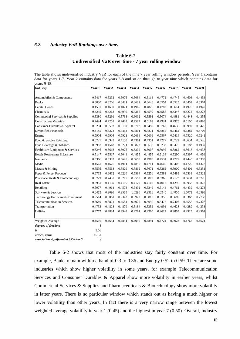
Table 6-2 Undiversified VaR over time - 7 year rolling window
The table shows undiversified industry VaR for each of the nine 7 year rolling window periods. Year 1 contains data for years 1-7. Year 2 contains data for years 2-8 and so on through to year nine which contains data for years 9-15. Industry Year 1 Year 2 Year 3 Year 4 Year 5 Year 6 Year 7 Year 8 Year 9
Automobiles & Components 0.5417 0.5232 0.5076 0.5084 0.5113 0.4772 0.4745 0.4603 0.4453Banks 0.3030 0.3206 0.3421 0.3622 0.3646 0.3554 0.3525 0.3452 0.3384Capital Goods 0.4591 0.4639 0.4821 0.4965 0.4826 0.4782 0.5614 0.4970 0.4949Chemicals 0.4215 0.4263 0.4090 0.4365 0.4599 0.4585 0.4346 0.4272 0.4273Commercial Services & Supplies 0.5380 0.5291 0.5763 0.6012 0.5591 0.5074 0.4981 0.4448 0.4355Construction Materials 0.4424 0.4251 0.4403 0.4587 0.5162 0.4924 0.4975 0.5100 0.4895Consumer Durables & Apparel 0.5294 0.5593 0.6159 0.6702 0.6498 0.6767 0.4630 0.6997 0.6425Diversified Financials 0.4145 0.4273 0.4453 0.4801 0.4871 0.4855 0.5462 0.5382 0.4706Energy 0.5904 0.5904 0.5921 0.5689 0.5608 0.5567 0.5419 0.5520 0.5241Food & Staples Retailing 0.3727 0.3943 0.4150 0.4361 0.4351 0.4277 0.3722 0.3634 0.3526Food Beverage & Tobacco 0.3987 0.4548 0.5221 0.5823 0.5532 0.5233 0.5476 0.5183 0.4937Healthcare Equipment & Services 0.5246 0.5618 0.6075 0.6302 0.6007 0.5992 0.5862 0.5613 0.4938Hotels Restaurants & Leisure 0.5147 0.5517 0.5043 0.4855 0.4855 0.5138 0.5290 0.5397 0.4056Insurance 0.5366 0.5392 0.5625 0.5650 0.4989 0.4531 0.4777 0.4440 0.5393Media 0.4561 0.4676 0.4911 0.4895 0.4711 0.4640 0.5406 0.4720 0.4378Metals & Mining 0.5595 0.5568 0.5829 0.5812 0.5671 0.5362 0.5900 0.5401 0.5351Paper & Forest Products 0.6713 0.6612 0.6220 0.5584 0.5256 0.5381 0.5485 0.6531 0.5321Pharmaceuticals & Biotechnology 0.6729 0.7437 0.8295 0.9552 0.8073 0.6368 0.7123 0.6631 0.5726Real Estate 0.3931 0.4139 0.4195 0.4179 0.4100 0.4012 0.4295 0.3958 0.3878Retailing 0.5077 0.4964 0.4578 0.5432 0.5349 0.5144 0.4762 0.4439 0.4273Software & Services 0.8412 0.9098 0.9515 1.0290 0.9316 0.8245 1.4855 1.5071 0.8393Technology Hardware & Equipment 0.9514 0.8861 0.9342 0.9973 0.9813 0.9356 0.8689 0.8363 0.7758Telecommunication Services 0.3640 0.3821 0.4584 0.4925 0.5090 0.5477 0.7407 0.6555 0.7328Transportation 0.4732 0.4828 0.4879 0.5184 0.5352 0.4991 0.4628 0.4289 0.4233Utilities 0.3777 0.3834 0.3948 0.4261 0.4390 0.4622 0.4803 0.4929 0.4561
Weighted Average 0.4516 0.4634 0.4851 0.4990 0.4891 0.4724 0.5023 0.4767 0.4624degrees of freedom 8K 5.56critical value 15.51association significant at 95% level? y
Table 6-2 shows that most of the industries stay fairly constant over time. For
example, Banks remain within a band of 0.3 to 0.36 and Energy 0.52 to 0.59. There are some
industries which show higher volatility in some years, for example Telecommunication
Services and Consumer Durables & Apparel show more volatility in earlier years, whilst
Commercial Services & Supplies and Pharmaceuticals & Biotechnology show more volatility
in latter years. There is no particular window which stands out as having a much higher or
lower volatility than other years. In fact there is a very narrow range between the lowest
weighted average volatility in year 1 (0.45) and the highest in year 7 (0.50). Overall, industry

16
VaR rankings show a significant association over time. We also tested diversified VaR over
time. Again, the rankings are found to be significantly constant over time.
Table 6-3
Historical VaR using 12 month data windows
The seven year rolling window approach shown in Table 6-2 could be a key factor in influencing the stability in VaR over time, as there is overlap on the data with this approach. Year 1 of the rolling window approach contains 6 of the same years as year 2, year 2 contains 6 of the same years as year 3 and so on. To assess the impact of this, the table below tests historical VaR using only 1 year periods, i.e. each year contains only the last 12 months data. Industry Year 1 Year 2 Year 3 Year 4 Year 5 Year 6 Year 7 Year 8 Year 9
Automobiles & Components 0.5660 0.5956 0.3913 0.4227 0.5943 0.5276 0.5440 0.4515 0.5093Banks 0.2439 0.2231 0.2387 0.3163 0.3506 0.3588 0.3620 0.3709 0.3785Capital Goods 0.3787 0.3775 0.3711 0.4980 0.4816 0.5460 0.5896 0.4580 0.4932Chemicals 0.4000 0.4106 0.3030 0.4108 0.5324 0.4911 0.4606 0.4107 0.4515Commercial Services & Supplies 0.4307 0.4084 0.4386 0.6297 0.5698 0.5393 0.5973 0.4648 0.4986Construction Materials 0.4804 0.3855 0.3992 0.3938 0.5390 0.5096 0.5342 0.5718 0.5968Consumer Durables & Apparel 0.4278 0.4819 0.3696 0.6513 0.6302 0.6748 0.4603 0.5344 0.5733Diversified Financials 0.4126 0.3434 0.3004 0.3842 0.4190 0.3782 0.5238 0.5093 0.4850Energy 0.5647 0.5411 0.4356 0.4795 0.4911 0.5356 0.6188 0.5970 0.5617Food & Staples Retailing 0.2886 0.2919 0.2382 0.3359 0.4519 0.4923 0.4114 0.3951 0.4072Food Beverage & Tobacco 0.3554 0.3490 0.2842 0.3503 0.3728 0.4576 0.5026 0.5636 0.6597Healthcare Equipment & Services 0.4614 0.4405 0.4601 0.5392 0.6170 0.5719 0.5830 0.5679 0.5129Hotels Restaurants & Leisure 0.3567 0.4369 0.4212 0.4873 0.4446 0.4740 0.5937 0.6012 0.4261Insurance 0.3493 0.3566 0.4143 0.5542 0.6270 0.4051 0.5228 0.3938 0.5728Media 0.3545 0.3514 0.3411 0.4357 0.4415 0.4612 0.6577 0.4856 0.4311Metals & Mining 0.5730 0.4394 0.4641 0.4957 0.6042 0.5218 0.6255 0.6545 0.6709Paper & Forest Products 0.5372 0.5809 0.4705 0.3982 0.4824 0.6036 0.6015 0.6815 0.5770Pharmaceuticals & Biotechnology 0.5491 0.5847 0.5905 0.9098 0.8307 0.7079 0.8229 0.8008 0.5872Real Estate 0.2823 0.2945 0.2904 0.3374 0.3587 0.4495 0.4622 0.4270 0.4312Retailing 0.4948 0.4515 0.3715 0.5082 0.5835 0.5670 0.6035 0.5276 0.4845Software & Services 0.5257 0.6471 0.5947 0.8394 0.9397 0.8152 1.2598 1.6003 0.8830Technology Hardware & Equipment 0.8440 0.6526 0.7582 1.1482 1.2236 1.2408 1.0945 0.9587 0.8250Telecommunication Services 0.3355 0.2447 0.2563 0.3352 0.3783 0.4965 0.8259 0.5483 0.7500Transportation 0.4009 0.4037 0.3366 0.4893 0.5449 0.5948 0.5507 0.4445 0.4458Utilities 0.3556 0.3457 0.3028 0.3527 0.3954 0.4883 0.5498 0.4952 0.4774
Weighted Average 0.3943 0.3580 0.3507 0.4297 0.4780 0.4734 0.5394 0.5091 0.5187degrees of freedom 8K 51.47critical value 15.51association significant at 95% level? n
We now see a greater variance in VaR over time. For example Banks, which had a
very narrow VaR range over time, now show a range from 22% in year 2 to 38% in year 9.
The weighted portfolio average is 35% in year 3 compared to 54% in year 7. We also see
some changes to the ranking order. For example, on the 7 year approach, Chemicals in year 5
had a more favourable VaR than Capital Goods and in year 7 Media had a more favourable
VaR than metals. These positions are reversed under the 1 year approach.
17
There is no significant association in rankings using 1 year windows. The fact that the
7 year window approach gives a different outcome to the 1 year approach has significant
implications for users of VaR methodology such as Banks. Whilst using longer periods of
data has some advantages, such as taking account of different business cycles, it is also
important to focus on the more current risks. It is therefore important to consider both short
and long periods, and also to use CVaR, to focus on extreme risks.
6.3. Association between diversified VaR and undiversified VaR.
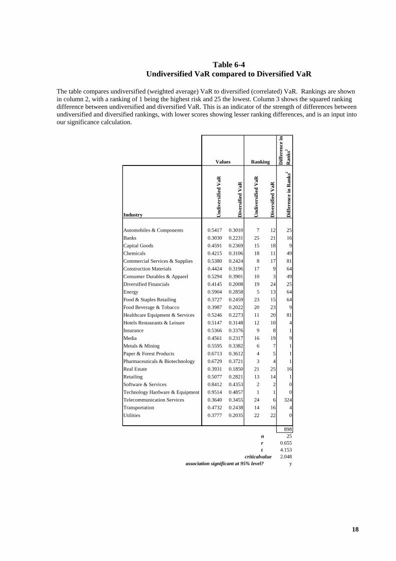
Table 6-4 shows there is an across the board noticeable reduction in risk when
correlation is applied to each industry. There is also a shift in rankings. For example,
Telecommunications has a low risk ranking on an undiversified basis, but shows very little
reduction in risk through diversification and thus has a higher risk ranking on a diversified
basis. Other industries have risk reduction through diversification which approximates the
overall portfolio average reduction, and thus retain a similar ranking on a diversified basis (for
example Insurance, Paper & Forest Products, and the Technology sectors). However, our
testing finds these differences not to be significant. We find significant association between
diversified and undiversified VaR.
18
Table 6-4 Undiversified VaR compared to Diversified VaR
The table compares undiversified (weighted average) VaR to diversified (correlated) VaR. Rankings are shown in column 2, with a ranking of 1 being the highest risk and 25 the lowest. Column 3 shows the squared ranking difference between undiversified and diversified VaR. This is an indicator of the strength of differences between undiversified and diversified rankings, with lower scores showing lesser ranking differences, and is an input into our significance calculation.
Diff
eren
ce in
R
anks
2
Industry Und
iver
sifie
d V
aR
Div
ersi
fied
VaR
Und
iver
sifie
d V
aR
Div
ersi
fied
VaR
Diff
eren
ce in
Ran
ks2
Automobiles & Components 0.5417 0.3010 7 12 25Banks 0.3030 0.2231 25 21 16Capital Goods 0.4591 0.2369 15 18 9Chemicals 0.4215 0.3106 18 11 49Commercial Services & Supplies 0.5380 0.2424 8 17 81Construction Materials 0.4424 0.3196 17 9 64Consumer Durables & Apparel 0.5294 0.3901 10 3 49Diversified Financials 0.4145 0.2008 19 24 25Energy 0.5904 0.2858 5 13 64Food & Staples Retailing 0.3727 0.2459 23 15 64Food Beverage & Tobacco 0.3987 0.2022 20 23 9Healthcare Equipment & Services 0.5246 0.2273 11 20 81Hotels Restaurants & Leisure 0.5147 0.3148 12 10 4Insurance 0.5366 0.3376 9 8 1Media 0.4561 0.2317 16 19 9Metals & Mining 0.5595 0.3382 6 7 1Paper & Forest Products 0.6713 0.3612 4 5 1Pharmaceuticals & Biotechnology 0.6729 0.3721 3 4 1Real Estate 0.3931 0.1850 21 25 16Retailing 0.5077 0.2821 13 14 1Software & Services 0.8412 0.4353 2 2 0Technology Hardware & Equipment 0.9514 0.4857 1 1 0Telecommunication Services 0.3640 0.3455 24 6 324Transportation 0.4732 0.2438 14 16 4Utilities 0.3777 0.2035 22 22 0
898n 25r 0.655t 4.153
criticalvalue 2.048 association significant at 95% level? y
RankingValues
19
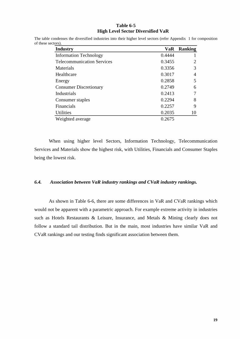
Table 6-5 High Level Sector Diversified VaR
The table condenses the diversified industries into their higher level sectors (refer Appendix 1 for composition of these sectors).
Industry VaR RankingInformation Technology 0.4444 1Telecommunication Services 0.3455 2Materials 0.3356 3Healthcare 0.3017 4Energy 0.2858 5Consumer Discretionary 0.2749 6Industrials 0.2413 7Consumer staples 0.2294 8Financials 0.2257 9Utilities 0.2035 10Weighted average 0.2675
When using higher level Sectors, Information Technology, Telecommunication
Services and Materials show the highest risk, with Utilities, Financials and Consumer Staples
being the lowest risk.
6.4. Association between VaR industry rankings and CVaR industry rankings.
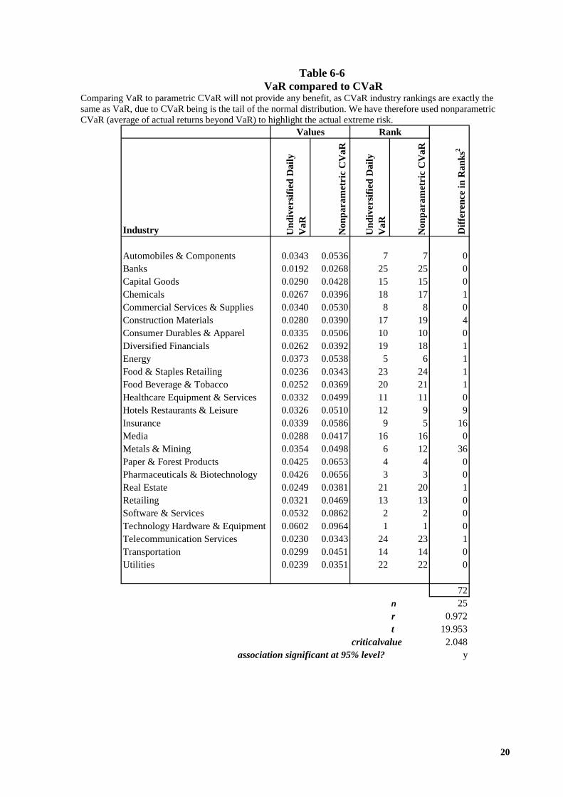
As shown in Table 6-6, there are some differences in VaR and CVaR rankings which
would not be apparent with a parametric approach. For example extreme activity in industries
such as Hotels Restaurants & Leisure, Insurance, and Metals & Mining clearly does not
follow a standard tail distribution. But in the main, most industries have similar VaR and
CVaR rankings and our testing finds significant association between them.
20
Table 6-6
VaR compared to CVaR Comparing VaR to parametric CVaR will not provide any benefit, as CVaR industry rankings are exactly the same as VaR, due to CVaR being is the tail of the normal distribution. We have therefore used nonparametric CVaR (average of actual returns beyond VaR) to highlight the actual extreme risk.
Industry Und
iver
sifie
d D
aily
V
aR
Non
para
met
ric
CV
aR
Und
iver
sifie
d D
aily
V
aR
Non
para
met
ric
CV
aR
Automobiles & Components 0.0343 0.0536 7 7 0Banks 0.0192 0.0268 25 25 0Capital Goods 0.0290 0.0428 15 15 0Chemicals 0.0267 0.0396 18 17 1Commercial Services & Supplies 0.0340 0.0530 8 8 0Construction Materials 0.0280 0.0390 17 19 4Consumer Durables & Apparel 0.0335 0.0506 10 10 0Diversified Financials 0.0262 0.0392 19 18 1Energy 0.0373 0.0538 5 6 1Food & Staples Retailing 0.0236 0.0343 23 24 1Food Beverage & Tobacco 0.0252 0.0369 20 21 1Healthcare Equipment & Services 0.0332 0.0499 11 11 0Hotels Restaurants & Leisure 0.0326 0.0510 12 9 9Insurance 0.0339 0.0586 9 5 16Media 0.0288 0.0417 16 16 0Metals & Mining 0.0354 0.0498 6 12 36Paper & Forest Products 0.0425 0.0653 4 4 0Pharmaceuticals & Biotechnology 0.0426 0.0656 3 3 0Real Estate 0.0249 0.0381 21 20 1Retailing 0.0321 0.0469 13 13 0Software & Services 0.0532 0.0862 2 2 0Technology Hardware & Equipment 0.0602 0.0964 1 1 0Telecommunication Services 0.0230 0.0343 24 23 1Transportation 0.0299 0.0451 14 14 0Utilities 0.0239 0.0351 22 22 0
72n 25r 0.972t 19.953
criticalvalue 2.048 association significant at 95% level? y
Diff
eren
ce in
Ran
ks2
RankValues
21
6.5. Industry CVaR rankings over time.
Table 6-7 Historical daily nonparametric CVaR
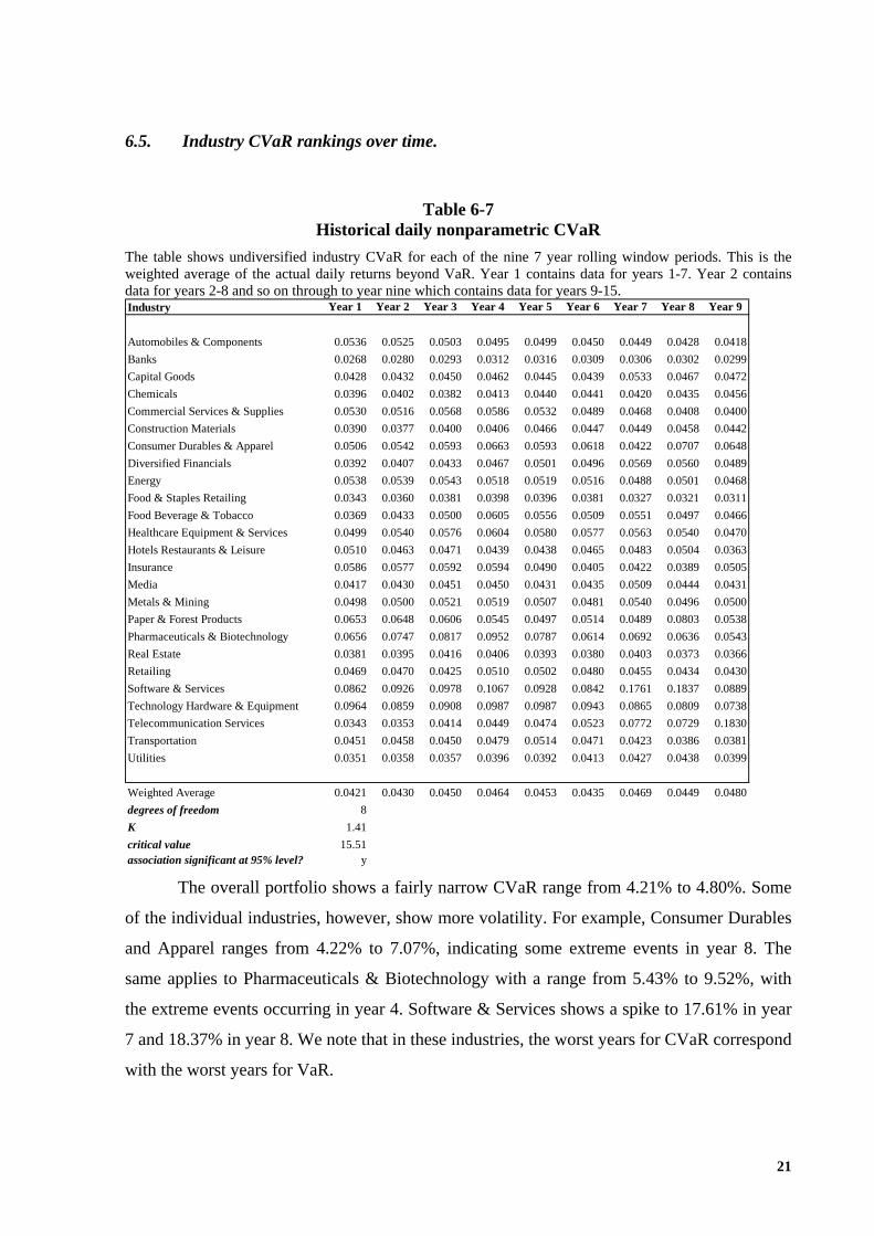
The table shows undiversified industry CVaR for each of the nine 7 year rolling window periods. This is the weighted average of the actual daily returns beyond VaR. Year 1 contains data for years 1-7. Year 2 contains data for years 2-8 and so on through to year nine which contains data for years 9-15. Industry Year 1 Year 2 Year 3 Year 4 Year 5 Year 6 Year 7 Year 8 Year 9
Automobiles & Components 0.0536 0.0525 0.0503 0.0495 0.0499 0.0450 0.0449 0.0428 0.0418Banks 0.0268 0.0280 0.0293 0.0312 0.0316 0.0309 0.0306 0.0302 0.0299Capital Goods 0.0428 0.0432 0.0450 0.0462 0.0445 0.0439 0.0533 0.0467 0.0472Chemicals 0.0396 0.0402 0.0382 0.0413 0.0440 0.0441 0.0420 0.0435 0.0456Commercial Services & Supplies 0.0530 0.0516 0.0568 0.0586 0.0532 0.0489 0.0468 0.0408 0.0400Construction Materials 0.0390 0.0377 0.0400 0.0406 0.0466 0.0447 0.0449 0.0458 0.0442Consumer Durables & Apparel 0.0506 0.0542 0.0593 0.0663 0.0593 0.0618 0.0422 0.0707 0.0648Diversified Financials 0.0392 0.0407 0.0433 0.0467 0.0501 0.0496 0.0569 0.0560 0.0489Energy 0.0538 0.0539 0.0543 0.0518 0.0519 0.0516 0.0488 0.0501 0.0468Food & Staples Retailing 0.0343 0.0360 0.0381 0.0398 0.0396 0.0381 0.0327 0.0321 0.0311Food Beverage & Tobacco 0.0369 0.0433 0.0500 0.0605 0.0556 0.0509 0.0551 0.0497 0.0466Healthcare Equipment & Services 0.0499 0.0540 0.0576 0.0604 0.0580 0.0577 0.0563 0.0540 0.0470Hotels Restaurants & Leisure 0.0510 0.0463 0.0471 0.0439 0.0438 0.0465 0.0483 0.0504 0.0363Insurance 0.0586 0.0577 0.0592 0.0594 0.0490 0.0405 0.0422 0.0389 0.0505Media 0.0417 0.0430 0.0451 0.0450 0.0431 0.0435 0.0509 0.0444 0.0431Metals & Mining 0.0498 0.0500 0.0521 0.0519 0.0507 0.0481 0.0540 0.0496 0.0500Paper & Forest Products 0.0653 0.0648 0.0606 0.0545 0.0497 0.0514 0.0489 0.0803 0.0538Pharmaceuticals & Biotechnology 0.0656 0.0747 0.0817 0.0952 0.0787 0.0614 0.0692 0.0636 0.0543Real Estate 0.0381 0.0395 0.0416 0.0406 0.0393 0.0380 0.0403 0.0373 0.0366Retailing 0.0469 0.0470 0.0425 0.0510 0.0502 0.0480 0.0455 0.0434 0.0430Software & Services 0.0862 0.0926 0.0978 0.1067 0.0928 0.0842 0.1761 0.1837 0.0889Technology Hardware & Equipment 0.0964 0.0859 0.0908 0.0987 0.0987 0.0943 0.0865 0.0809 0.0738Telecommunication Services 0.0343 0.0353 0.0414 0.0449 0.0474 0.0523 0.0772 0.0729 0.1830Transportation 0.0451 0.0458 0.0450 0.0479 0.0514 0.0471 0.0423 0.0386 0.0381Utilities 0.0351 0.0358 0.0357 0.0396 0.0392 0.0413 0.0427 0.0438 0.0399
Weighted Average 0.0421 0.0430 0.0450 0.0464 0.0453 0.0435 0.0469 0.0449 0.0480degrees of freedom 8K 1.41critical value 15.51association significant at 95% level? y
The overall portfolio shows a fairly narrow CVaR range from 4.21% to 4.80%. Some
of the individual industries, however, show more volatility. For example, Consumer Durables
and Apparel ranges from 4.22% to 7.07%, indicating some extreme events in year 8. The
same applies to Pharmaceuticals & Biotechnology with a range from 5.43% to 9.52%, with
the extreme events occurring in year 4. Software & Services shows a spike to 17.61% in year
7 and 18.37% in year 8. We note that in these industries, the worst years for CVaR correspond
with the worst years for VaR.
22
These differences over time are not found to be significant and we find CVaR to be
significantly constant over time.
7. Sector Indices
Besides just using risk measurements for capital adequacy purposes, Banks use them
for a number of other purposes such as risk concentration limits and setting policies. Banks
have traditionally obtained this industry information through their own or external
macroeconomic research. The VaR and CVaR measurements we have provided can assist
Banks in this process by being able to identify the relative risk of Australian industries, or
they can use the methodology to derive their own measurements. Banks often group risk
measurements into categories (such as high, medium, low) for purposes of simplicity. For
example, lower concentration limits may be allowed for a low risk industry than for a low risk
one. Banks could use the actual VaR / CVaR measurements which we have provided.
Alternatively risk indices could be used, or risk categories (high, low, etc). In Table 7-1, we
provide for all of these options.

23
Table 7-1 Risk Measurements, indices and categories
The first column shows the industry. The second column shows the diversified VaR values which we have already calculated. The third column, the industry risk index, shows the relative risk of each industry to the mean, where 1 = average risk, > 1 = higher than average risk and < 1 = lower than average risk. The measurement is obtained by industry VaR divided by portfolio mean VaR. This measurement is useful in that it is very easy to tell the relative risk from the measurement (for example a measurement of 0.5 is an industry with half the average risk, and 2 is double the average). It also facilitates comparison between models and comparison between VaR and CVaR (if all of these have a relative index calculated). In column 3 we show the relative risk in categories of low (20th percentile), medium-low (>20th to 40th percentile), medium >40th - 60th percentile, medium-high (>60th – 80th percentile) and high (>80th percentile).
Industry Div
ersi
fied
Port
folio
95%
V
aR
Indu
stry
Ris
k In
dex
Rel
ativ
e R
isk
Real Estate 0.18495 0.63Diversified Financials 0.20082 0.69Food Beverage & Tobacco 0.20220 0.69Utilities 0.20349 0.69Banks 0.22305 0.76Healthcare Equipment & Services 0.22731 0.78Media 0.23173 0.79Capital Goods 0.23692 0.81Commercial Services & Supplies 0.24239 0.83Transportation 0.24384 0.83Food & Staples Retailing 0.24593 0.84Retailing 0.28206 0.96Energy 0.28578 0.98Automobiles & Components 0.30102 1.03Chemicals 0.31059 1.06Hotels Restaurants & Leisure 0.31481 1.07Construction Materials 0.31955 1.09Insurance 0.33763 1.15Metals & Mining 0.33825 1.15Telecommunication Services 0.34548 1.18Paper & Forest Products 0.36123 1.23Pharmaceuticals & Biotechnology 0.37209 1.27Consumer Durables & Apparel 0.39006 1.33Software & Services 0.43535 1.49Technology Hardware & Equipment 0.48570 1.66
Low
Med
ium
-Low
Med
ium
Med
ium
-Hig
hH
igh

24
Table 7-2
Inclusion of CVaR into risk category allocation. It may also be prudent for a user of VaR indices, such as Banks, to bring CVaR into category allocation. An industry may have a relatively low VaR, but a high CVaR due to extreme loss potential. The use of CVaR is a conservative measure focussing on the top end of the risk. Following this conservative focus, we have chosen the overall risk category as being the highest risk category between VaR and CVaR. So if an industry has a VaR risk of medium, but a CVaR risk of medium-high, it is allocated to the medium-high category. Thus, using this approach, the inclusion of CVaR results in a downward shift of risk categories towards the higher risk buckets.
Dai
ly D
iver
sifie
d Po
rtfo
lio 9
5% V
aR
Indu
stry
VaR
Inde
x
Var
Ris
k C
ateg
ory
CV
aR
Indu
stry
CV
aR In
dex
CV
aR R
isk
Cat
egor
y
Food Beverage & Tobacco 0.0128 0.69 Low 0.0369 0.75 Low lowUtilities 0.0129 0.69 Low 0.0351 0.71 Low lowBanks 0.0141 0.76 Low 0.0268 0.54 Low lowReal Estate 0.0117 0.63 Low 0.0381 0.77 Medium-Low medium-lowDiversified Financials 0.0127 0.69 Low 0.0392 0.79 Medium-Low medium-lowMedia 0.0147 0.79 Medium-Low 0.0417 0.85 Medium-Low medium-lowHealthcare Equipment & Services 0.0144 0.78 Medium-Low 0.0499 1.01 Medium mediumCapital Goods 0.0150 0.81 Medium-Low 0.0428 0.87 Medium mediumTransportation 0.0154 0.83 Medium-Low 0.0451 0.91 Medium mediumFood & Staples Retailing 0.0156 0.84 Medium 0.0343 0.69 Low mediumRetailing 0.0178 0.96 Medium 0.0469 0.95 Medium mediumChemicals 0.0196 1.06 Medium 0.0396 0.80 Medium-Low mediumCommercial Services & Supplies 0.0153 0.83 Medium-Low 0.0530 1.07 Medium-High medium-highEnergy 0.0181 0.98 Medium 0.0538 1.09 Medium-High medium-highAutomobiles & Components 0.0190 1.03 Medium 0.0536 1.09 Medium-High medium-highHotels Restaurants & Leisure 0.0199 1.07 Medium-High 0.0510 1.03 Medium-High medium-highConstruction Materials 0.0202 1.09 Medium-High 0.0390 0.79 Medium-Low medium-highMetals & Mining 0.0214 1.15 Medium-High 0.0498 1.01 Medium medium-highTelecommunication Services 0.0219 1.18 Medium-High 0.0343 0.70 Low medium-highInsurance 0.0214 1.15 Medium-High 0.0586 1.19 High highPaper & Forest Products 0.0228 1.23 High 0.0653 1.32 High highPharmaceuticals & Biotechnology 0.0235 1.27 High 0.0656 1.33 High highConsumer Durables & Apparel 0.0247 1.33 High 0.0506 1.03 Medium-High highSoftware & Services 0.0275 1.49 High 0.0862 1.75 High highTechnology Hardware & Equipment 0.0307 1.66 High 0.0964 1.95 High high
Var CVar
Com
bine
d R
isk
Cat
egor
y
Industry
8. Conclusions
The objectives of the study were to provide market industry VaR and CVaR
measurements, to compare VaR and CVaR rankings between industries over time, to compare
diversified (correlated) and undiversified industry VaR rankings, to compare parametric and
nonparametric CVaR rankings for each industry. We find the Technology Sectors to show the
highest risk, and lowest risk in the Financial and Utility Sectors. Although some industries
show differences between diversified and undiversified risk (such as Telecommunications
25
showing a much higher risk ranking on a diversified basis), overall there is found to be
significant association between diversified and undiversified VaR.
CVaR identifies extreme risk. There are some ranking differences between VaR and
(nonparametric) CVaR, such as Insurance showing a relatively higher CVaR than VaR, but
overall CVaR rankings show significant similarities to VaR rankings. There is also found to
be significant association between parametric and nonparametric CVaR. There is found to be
significant ranking correlation over time for both VaR and CVaR using our 7 year rolling
window approach. When 1 year data frames are used, no association over time was found.
This highlights the importance of using both short and long time frames in order to cover
different economic cycles as well as consider current conditions.
Using the 7 year time frames shows significant association between the outcomes of
all the metrics used in this study. We conclude that, provided sufficiently lengthy time periods
are used, these metrics show robustness and consistency over time and across industry sectors.
With the increased momentum in risk modelling brought about by the Basel II Accord,
and the relative lack of VaR and CVaR studies in Australia, there is significant scope for
additional studies on this topic, particularly with regards to CVaR, for both market and credit
risk. The examination of credit VaR and CVaR in an Australian context will be discussed by
the same authors in a separate paper.
26
9. REFERENCES
Alexander, G. J., & Baptista, A. M. (2003). CVaR as a measure of Risk: Implications for Portfolio Selection: Working Paper, School of Management, University of Minnesota.
Alexander, S., Coleman, T. F., & Li, Y. (2003). Derivative Portfolio Hedging Based on CVaR. In G. Szego (Ed.), New Risk Measures in Investment and Regulation: John Wiley and Sons Ltd.
Andersson, F., Mausser, H., Rosen, D., & Uryasev, S. (2000). Credit Risk Optimization with Conditional Value-at Risk criterion, from http://www.ise.ufl.edu/uryasev/Credit_risk_optimization.pdf
Artzner, P., Delbaen, F., Eber, J., & Heath, D. (1999). Coherent Measures of Risk. Mathematical Finance, Vol. 9, pp.203-228.
Artzner, P., Delbaen, F., Eber, J. M., & Heath, D. (1997). Thinking Coherently. Risk, Vol. 10, pp.68-71.
Australian Stock Exchange. (2006). What is GICS?, from http://www.asx.com.au/research/indices/gics.htm
Bank for International Settlements. (2004). Basel II: International Convergence of Capital Measurement and Capital Standards: a Revised Framework, from www.bis.org/publ/bcbs107.htm
Beder, T. (1995). VaR: Seductive but Dangerous. Financial Analysts Journal, Vol. 51(5), pp.12-25.
Brailsford, T., & Heaney, R. (1998). Investments: Concepts and Applications in Australia. Marrickville: Harcourt Brace & Company Australia, pp.229-244.
Bucay, N., & Rosen, D. (1999). Case Study. ALGO Research Quarterly, Vol.2(1), pp.9-29.
Duffie, D., & Pan, J. (1997). An Overview of Value at Risk. Journal of Derivatives, Vol.4, pp.7-49.
Engel, J., & Gizycki, M. (1999). Conservatism, Accuracy and Efficiency: Comparing Value at Risk Models: APRA, wp0002.
Gizycki, M., & Hereford, M. (1999). Assessing the Dispersion in Banks' Estimates of Market Risk: The Results of a Value at Risk survey: APRA, wp0001.
Global Derivatives Study Group. (1993). Derivatives: Practices and Principles. Technical Report, Group of Thirty, Washington D.C.
Harper, D. (2004). The Uses and Limits of Volatility, from www.investopedia.com/articles/04/021804.asp
Huang, A. (2000). A Comparison of Value at Risk Approaches and a New Method with Extreme Value Theory and Kernel Estimator, from http://www.cm.yzu.edu.tw/FN/ENG/F_Research/topic/Value%20at%20Risk%20with%20Kernel%20Estimator.pdf
J.P. Morgan, & Reuters. (1996). RiskMetrics Technical Document, from www.riskmetrics.com/rmcovv.html
27
Jorion, P. (1996). Value at Risk: The New Benchmark for Controlling Dervative Risk: Irwin Professional Publishing.
Kast, R., Luciano, E., & Peccati, L. (1998). VaR and Optimisation. Paper presented at the 2nd International Workshop on Preferences, Trento, Italy.
Lee, C. F., Lee, J. C., & Lee, A. C. (2000). Statistics for Business and Financial Economics (2nd ed.). Singapore: World Scientific Publishing Co. Pte Ltd., pp.759-784.
Litterman, R. (1997a). Hot Spots and Hedges (I). Risk, Vol. 10(3), pp. 42-45.
Litterman, R. (1997b). Hot Spots and Hedges (II). Risk, Vol. 10(5), pp.38-42.
Lucas, A., & Klausen, P. (1998). Extreme Returns, Downside Risk and Optimal Asset Allocation. Journal of Portfolio Management, Vol. 25(1), pp.71-79.
Mauser, H., & Rosen, D. (1999). Beyond VaR: From Measuring Risk to Managing Risk. ALGO Research Quarterly, Vol.1(2), pp.5-20.
McKay, R., & Keefer, T. E. (1996). VaR is a Dangerous Technique. Corporate Finance, Searching for Sysrtems Integration Supplement, pp.30.
Miller, M., Muthuswamy, J., & Whaley, R. (1994). Mean Reversion of Standard & Poor's 500 Index Basis Changes: Arbitrage Induced or Statistical Illusion? Journal of Finance, Vol.49(2), pp.479-513.
Pflug, G. (2000). Some Remarks on Value-at-Risk and Conditional-Value-at-Risk. In R. Uryasev (Ed.), Probabilistic Constrained Optimisation: Methodology and Applications. Dordrecht, Boston: Kluwer Academic Publishers.
Pritsker, M. (1997). Evaluating Value-at-Risk Methodologies: Accuracy versus Computational Time. Journal of Financial Services Research, Vol.12(2/3), pp.201-242.
Rockafellar, R. T., & Uryasev, S. (2002). Conditional Value-at-Risk for General Loss Distributions. Journal of Banking and Finance, Vol.26, pp.1443-1471.
Rockafellar, R. T., Uryasev, S., & Zabarankin, M. (2006). Master Funds in Portfolio Analysis with General Deviation Measures. Journal of Banking and Finance, Vol.30(2).
Siegel, S., & Castellan, N. (1988). Nonparametric Statistics for the Behavioural Sciences. Singapore: McGraw-Hill, pp.206-244.
Stambaugh, F. (1996). Risk and Value at Risk. European Management Journal, Vol.14(6), pp.612-621.
Standard & Poor's. (2006). Indices, from http://www2.standardandpoors.com/portal/site/sp/en/au/page.family/indices_ei_au/2,3,2,8,0,0,0,0,0,0,0,0,0,0,0,0.html
Sy. (2006). On the Coherence of VaR Measure for Levy Stable Distributions: APRA, wp.2006-02.
Uryasev, S., & Rockafellar, R. T. (1999). Optimisation of Conditional Value-at-Risk, from www.ise.ufl.edu/uryasev/CVar1_JOR.pdf
28
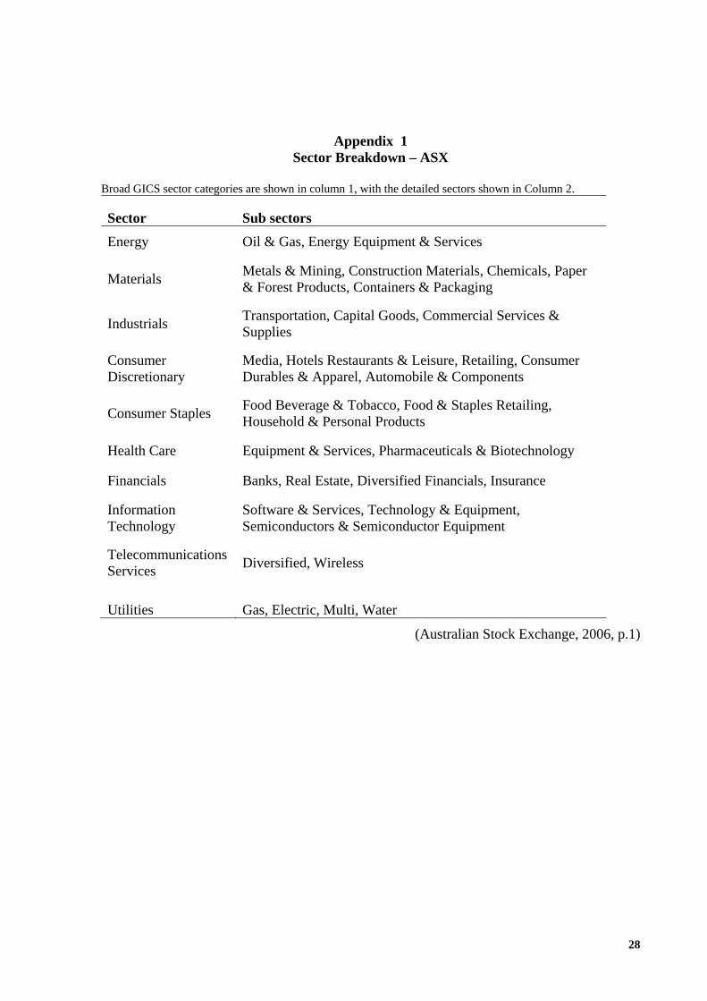
Appendix 1 Sector Breakdown – ASX
Broad GICS sector categories are shown in column 1, with the detailed sectors shown in Column 2.
Sector Sub sectors
Energy Oil & Gas, Energy Equipment & Services
Materials Metals & Mining, Construction Materials, Chemicals, Paper & Forest Products, Containers & Packaging
Industrials Transportation, Capital Goods, Commercial Services & Supplies
Consumer Discretionary
Media, Hotels Restaurants & Leisure, Retailing, Consumer Durables & Apparel, Automobile & Components
Consumer Staples Food Beverage & Tobacco, Food & Staples Retailing, Household & Personal Products
Health Care Equipment & Services, Pharmaceuticals & Biotechnology
Financials Banks, Real Estate, Diversified Financials, Insurance
Information Technology
Software & Services, Technology & Equipment, Semiconductors & Semiconductor Equipment
Telecommunications Services Diversified, Wireless
Utilities
Gas, Electric, Multi, Water
(Australian Stock Exchange, 2006, p.1)
29
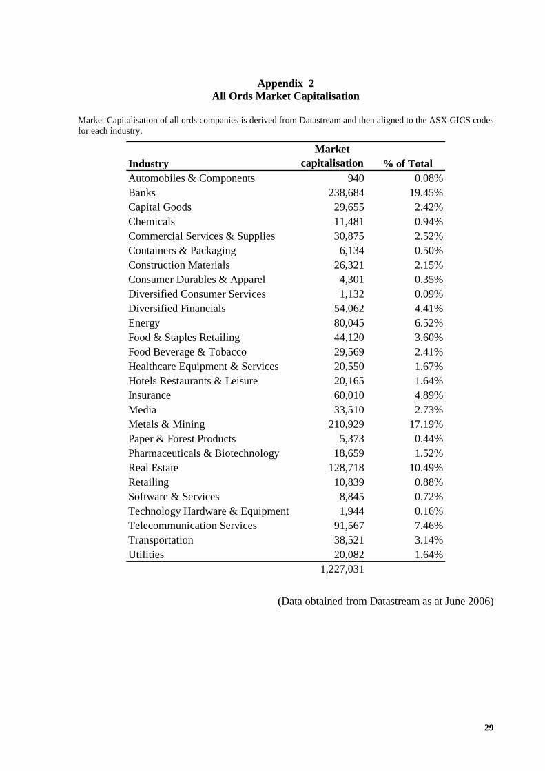
Appendix 2 All Ords Market Capitalisation
Market Capitalisation of all ords companies is derived from Datastream and then aligned to the ASX GICS codes for each industry.
IndustryMarket
capitalisation % of TotalAutomobiles & Components 940 0.08%Banks 238,684 19.45%Capital Goods 29,655 2.42%Chemicals 11,481 0.94%Commercial Services & Supplies 30,875 2.52%Containers & Packaging 6,134 0.50%Construction Materials 26,321 2.15%Consumer Durables & Apparel 4,301 0.35%Diversified Consumer Services 1,132 0.09%Diversified Financials 54,062 4.41%Energy 80,045 6.52%Food & Staples Retailing 44,120 3.60%Food Beverage & Tobacco 29,569 2.41%Healthcare Equipment & Services 20,550 1.67%Hotels Restaurants & Leisure 20,165 1.64%Insurance 60,010 4.89%Media 33,510 2.73%Metals & Mining 210,929 17.19%Paper & Forest Products 5,373 0.44%Pharmaceuticals & Biotechnology 18,659 1.52%Real Estate 128,718 10.49%Retailing 10,839 0.88%Software & Services 8,845 0.72%Technology Hardware & Equipment 1,944 0.16%Telecommunication Services 91,567 7.46%Transportation 38,521 3.14%Utilities 20,082 1.64%
1,227,031
(Data obtained from Datastream as at June 2006)
Recommended

![Value-at-Riskvs.ConditionalValue-at-Riskin ...Conditional value-at-risk (CVaR), introduced by Rockafellar and Uryasev [19], is a popular tool for managing risk. CVaR approximately](https://img.pdfslide.net/doc/110x75/5e7993838dda0e210b3916b7/value-at-conditional-value-at-risk-cvar-introduced-by-rockafellar-and-uryasev.jpg)