Embed Size (px)
Citation preview
Government Macroeconomic Policy
• Definition and functions of money• Money is anything that is generally acceptable
as a means of payment. Money serves three separate functions in any economy. It provides:
• A means of payment (exchange); whenever items are bought and sold.
• A store of (value) normally an attractive store of purchasing power during the period between the time it is earned and the time it is spent.
• A unit (measure of value) of account that allows all products to be valued consistently against a common measure.
The supply of money
• The supply of money is made up of currency and deposits with financial institutions.
• Currency includes paper notes and coins such as currency bills, issued by the central bank.
• However, there are several types of deposits. Some deposits give depositors immediate access to their money. They are called demand deposits and take the form of current and personal chequing accounts. This form of deposit is almost as liquid as money.
The supply of money
• Another popular form of deposit is known as saving or notice deposits, from which the depositor may officially withdraw funds only after giving notice to the financial institution. Notice deposits typically pay a higher rate of interest but limit or exclude cheque writing.
• A term / fixed deposit account is another form of deposit that entitles the holder to a higher rate of interest. A contractual condition of placing funds in a term deposit is that the depositor does not withdraw from that account for a specified period of time.
The supply of money
• Equation (1) below defines the money supply in a generic form:
• Ms= CU + D (1)• Where CU stands for currency in the hands of
public, D, deposits with banks, and Ms for the money supply.
• Several types of deposits also implies there are several different measures of money.
Measures of money
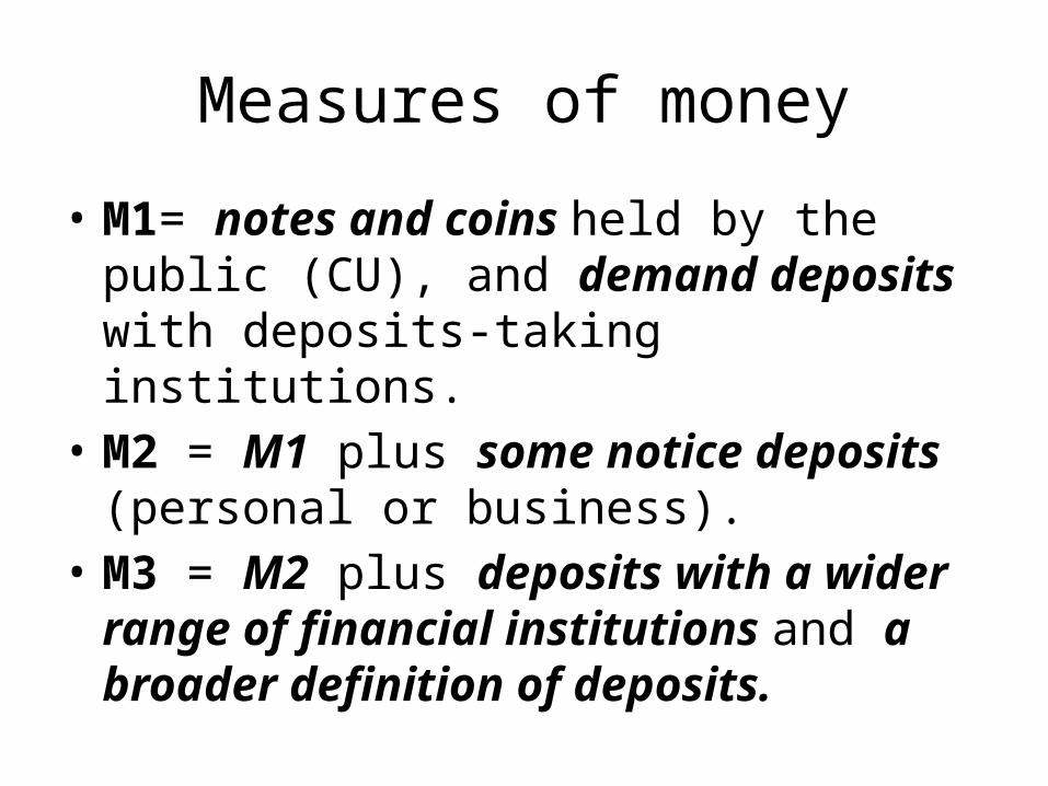
• M1= notes and coins held by the public (CU), and demand deposits with deposits-taking institutions.
• M2 = M1 plus some notice deposits (personal or business).
• M3 = M2 plus deposits with a wider range of financial institutions and a broader definition of deposits.
Motives for demanding money
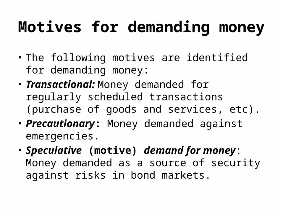
• The following motives are identified for demanding money:
• Transactional: Money demanded for regularly scheduled transactions (purchase of goods and services, etc).
• Precautionary: Money demanded against emergencies.
• Speculative (motive) demand for money: Money demanded as a source of security against risks in bond markets.
Motives for demanding money
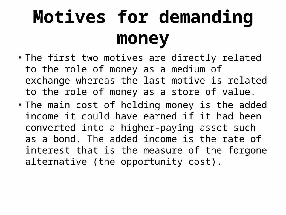
• The first two motives are directly related to the role of money as a medium of exchange whereas the last motive is related to the role of money as a store of value.
• The main cost of holding money is the added income it could have earned if it had been converted into a higher-paying asset such as a bond. The added income is the rate of interest that is the measure of the forgone alternative (the opportunity cost).
Bonds
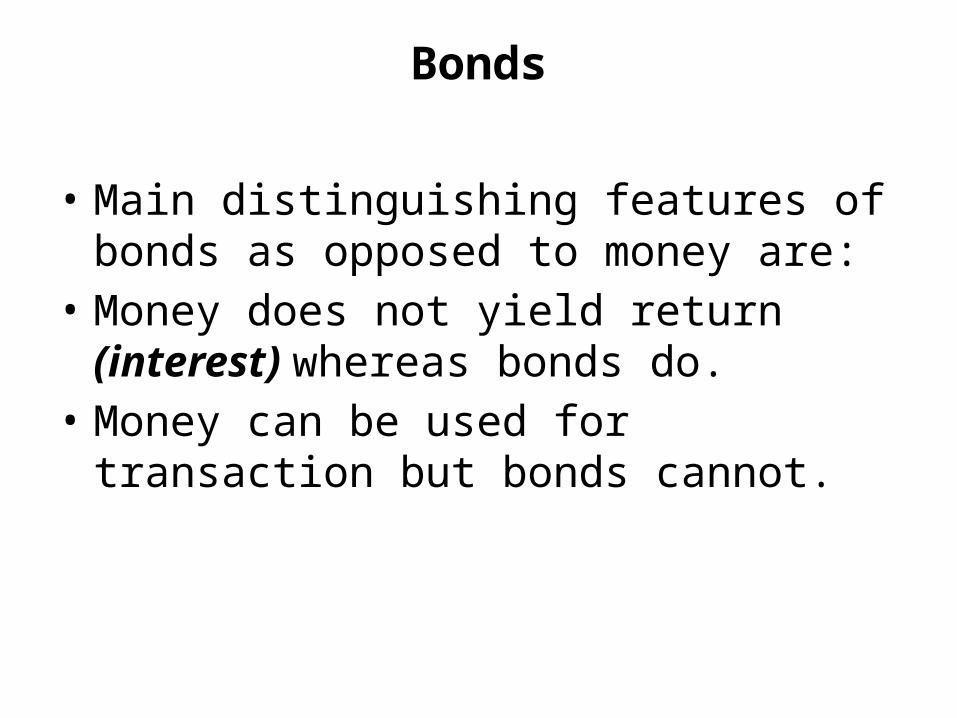
• Main distinguishing features of bonds as opposed to money are:
• Money does not yield return (interest) whereas bonds do.
• Money can be used for transaction but bonds cannot.
Bonds
• Bonds are formal contracts that set out the amount borrowed, by whom, for what period of time, and at what interest rate. Most bonds promise to pay an agreed-upon interest rate per period for the duration of the bond and also to pay back the bondholder the principal of the bond at its maturity. Bonds are also attractive assets because they can be easily bought and sold before their term has ended.
Bonds
• This way, they offer liquidity as well as relatively high rates of return in exchange for the risk associated with changes in bond prices. Therefore, for individuals who hold wealth, bonds offer the likeliest alternative to holding money for individuals who have a favourable view of the trade-off between bonds’ higher rates of return and higher risk.
Bonds
• The table below presents annual average
rates for a number of the Government of
Canada’s key interest rates. The rates in this
table show interest on short and long-term
instruments.
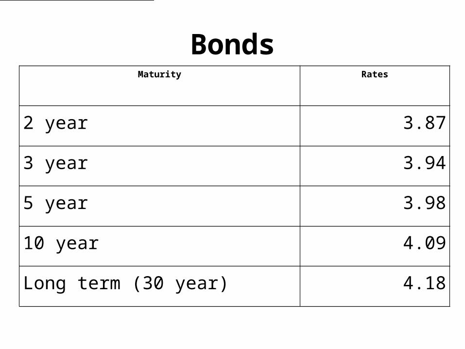
BondsMaturity Rates
2 year 3.87
3 year 3.94
5 year 3.98
10 year 4.09
Long term (30 year) 4.18
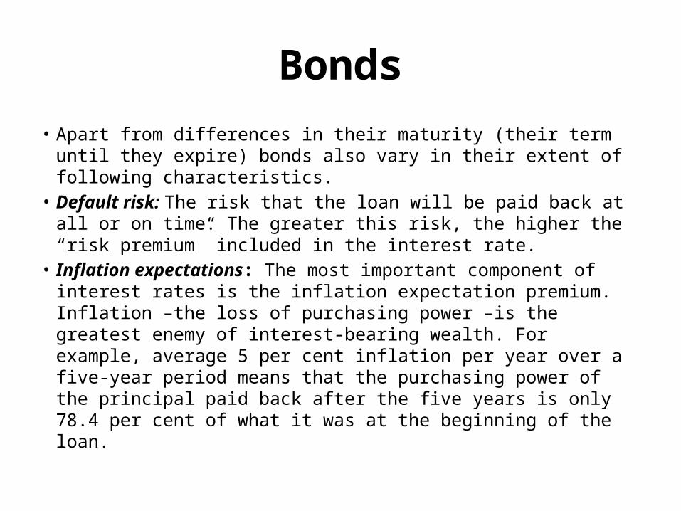
Bonds• Apart from differences in their maturity (their term until they
expire) bonds also vary in their extent of following characteristics.• Default risk: The risk that the loan will be paid back at all or on
time. The greater this risk, the higher the “risk premium” included in the interest rate.
• Inflation expectations: The most important component of interest rates is the inflation expectation premium. Inflation –the loss of purchasing power –is the greatest enemy of interest-bearing wealth. For example, average 5 per cent inflation per year over a five-year period means that the purchasing power of the principal paid back after the five years is only 78.4 per cent of what it was at the beginning of the loan.
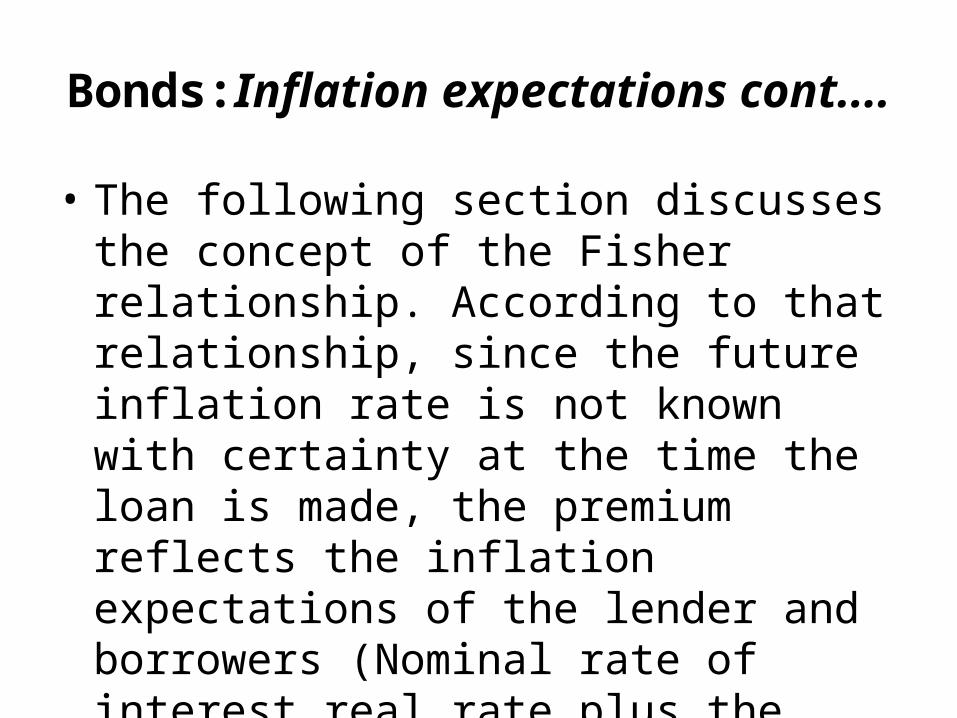
Bonds:Inflation expectations cont....
• The following section discusses the concept of the Fisher relationship. According to that relationship, since the future inflation rate is not known with certainty at the time the loan is made, the premium reflects the inflation expectations of the lender and borrowers (Nominal rate of interest real rate plus the expected inflation rate.)
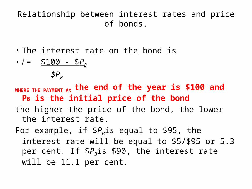
Relationship between interest rates and price of bonds.
• The interest rate on the bond is• i = $100 - $PB
$PB
WHERE THE PAYMENT At the end of the year is $100 and PB is the initial price of the bond
the higher the price of the bond, the lower the interest rate.
For example, if $PBis equal to $95, the interest rate will be equal to $5/$95 or 5.3 per cent. If $PBis $90, the interest rate will be 11.1 per cent.
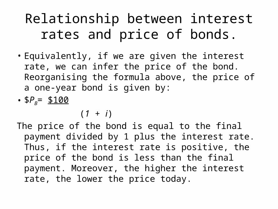
Relationship between interest rates and price of bonds.
• Equivalently, if we are given the interest rate, we can infer the price of the bond. Reorganising the formula above, the price of a one-year bond is given by:
• $PB= $100
(1 + i)The price of the bond is equal to the final payment
divided by 1 plus the interest rate. Thus, if the interest rate is positive, the price of the bond is less than the final payment. Moreover, the higher the interest rate, the lower the price today.
Bonds
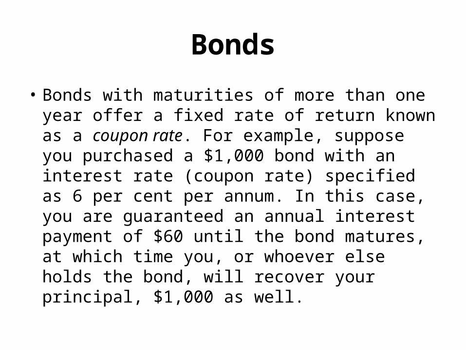
• Bonds with maturities of more than one year offer a fixed rate of return known as a coupon rate. For example, suppose you purchased a $1,000 bond with an interest rate (coupon rate) specified as 6 per cent per annum. In this case, you are guaranteed an annual interest payment of $60 until the bond matures, at which time you, or whoever else holds the bond, will recover your principal, $1,000 as well.
Financial systems
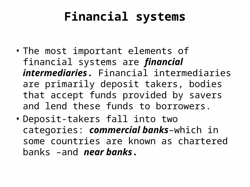
• The most important elements of financial systems are financial intermediaries. Financial intermediaries are primarily deposit takers, bodies that accept funds provided by savers and lend these funds to borrowers.
• Deposit-takers fall into two categories: commercial banks–which in some countries are known as chartered banks –and near banks.
Commercial banks
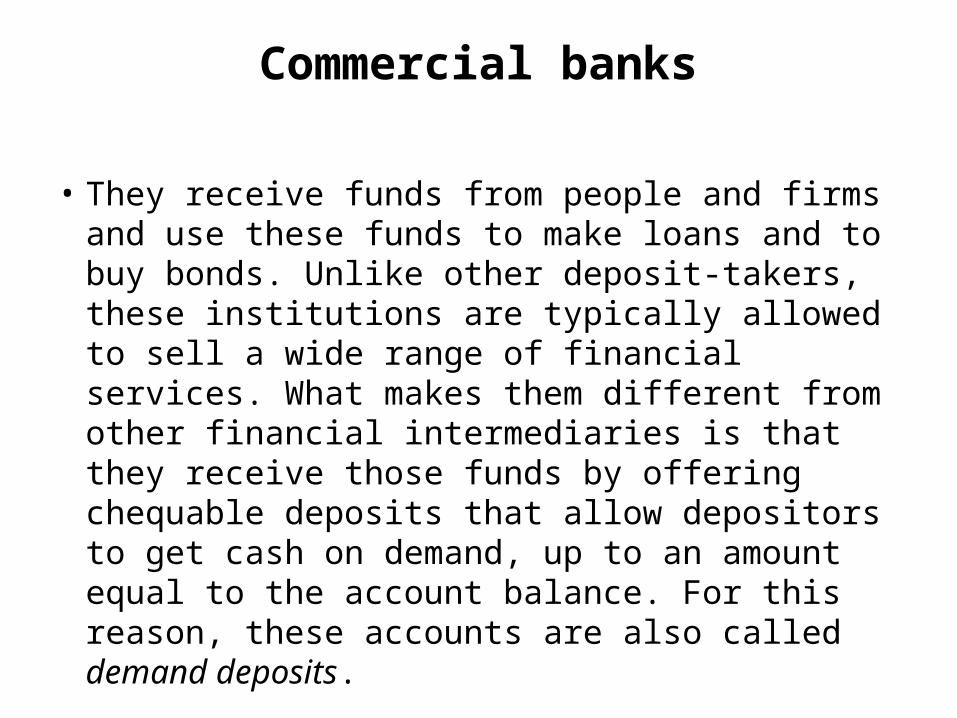
• They receive funds from people and firms and use these funds to make loans and to buy bonds. Unlike other deposit-takers, these institutions are typically allowed to sell a wide range of financial services. What makes them different from other financial intermediaries is that they receive those funds by offering chequable deposits that allow depositors to get cash on demand, up to an amount equal to the account balance. For this reason, these accounts are also called demand deposits.
Balance sheet
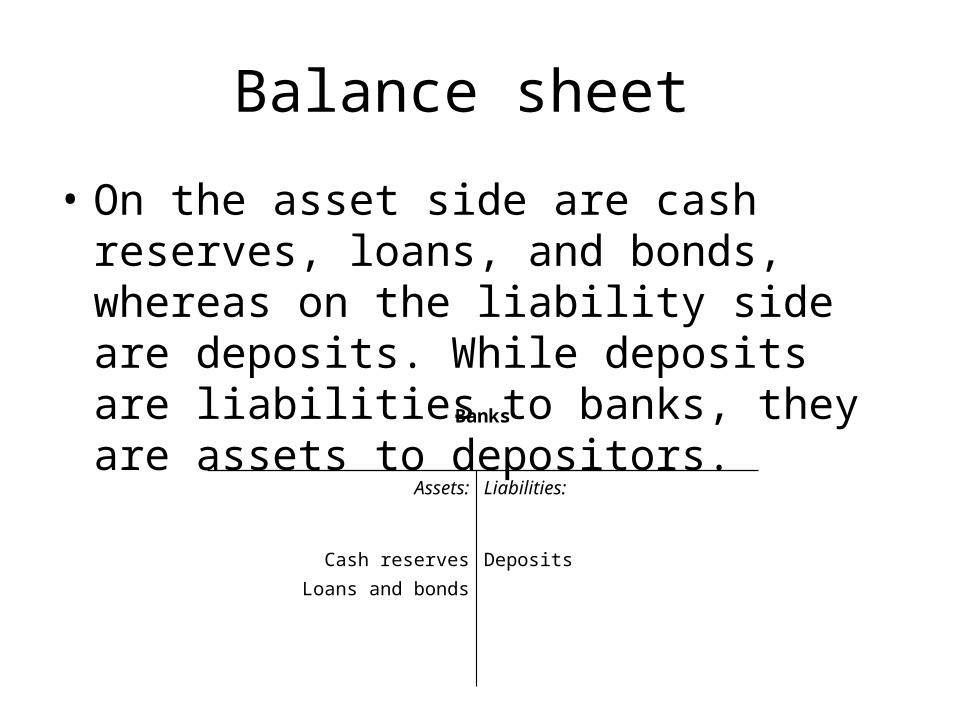
• On the asset side are cash reserves, loans, and bonds, whereas on the liability side are deposits. While deposits are liabilities to banks, they are assets to depositors.
Banks
Assets: Liabilities:
Cash reservesLoans and bonds
Deposits
Near banks
• They have more specialised financial services. E.g. trust companies, mortgage and loan companies, credit unions and other forms of government as well as private savings and loan associations. They now compete with commercial banks by taking deposits and granting loans, mainly to households. There are also Insurance companies and Investment dealers
Cash reserves
• Banks are required to hold reserves as a percentage of their deposits. These reserves are known as required reserves (or legal reserves): the minimum amount of reserves that banks by regulations must hold against deposits.
• Fractional reserve banking system- banks do not hold the whole of their total deposits as reserves but rather a fraction called the reserve requirement (r.r.) ratio.
The banking (money) multiplier
• When banks hold $100 billion in deposits for $10 billion reserves, the reserve ratio is 10 per cent (10/100). The banking multiplier just turns this idea around. If the banking system as a whole holds a total of $10 billion in reserves, it can have only $100 billion in deposits. In other words, if rr is the ratio of reserves to deposits for all banks, 10 per cent in this case, then the ratio of deposits to reserves in the banking system (that is, the banking multiplier) must be 1/rr, 10.
Central bank
• Issue currency.... This refers to supply notes and coins into the economy
• Act as the banker to commercial banks. the central bank holds deposits for commercial banks as commercial banks do for the public. These deposits at the central bank enable commercial banks to make payments to one another. More importantly, central banks act as the lender of last resort by extending short-term loans to banks that may be in a credit crunch.
Central bank
• Act as the banker to the government.... manages the government bank account, which is held with the central bank, and handles its debt.
• Control money stock, which is the most important task of the central bank. The decision by the central bank concerning the money supply is referred to as monetary policy.
• Currencies issued by central banks are referred to as fiat money –money that has no intrinsic value.
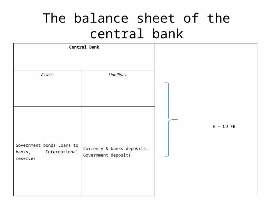
The balance sheet of the central bankCentral Bank
H = CU +R
Assets: Liabilities:
Government bonds,Loans to banks, International
reserves
Currency & banks deposits, Government deposits
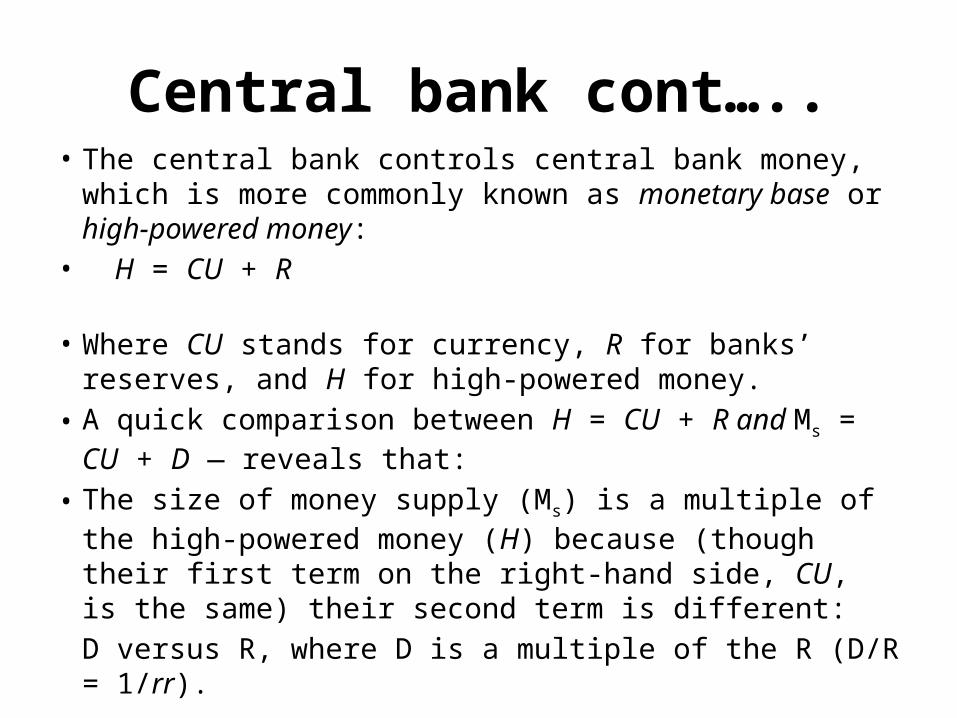
Central bank cont…..• The central bank controls central bank money, which is
more commonly known as monetary base or high-powered money:
• H = CU + R • Where CU stands for currency, R for banks’ reserves, and
H for high-powered money.• A quick comparison between H = CU + R and Ms = CU + D
— reveals that:• The size of money supply (Ms) is a multiple of the high-
powered money (H) because (though their first term on the right-hand side, CU, is the same) their second term is different:D versus R, where D is a multiple of the R (D/R = 1/rr).
Central bank cont…..
• The central bank controls only part of the money supply directly. That is currency (CU). Its controls of the rest of money supply –deposits (D) –are indirect.
Monetary policy
• Tools of monetary policy• Open-market operations- the central bank
changes the stock of money in the economy by buying and selling bonds in the bond market. . Such operations are called open market operations, because they take place in the “open market” for bonds.
Open-market operations cont….
Open-market operations cont….
• If the central bank increases the supply of money, it is called an expansionary monetary policy.
• When, instead, the central bank wants to decrease the supply of money, it does an open market sale of government bonds called contractionary monetary policy.
Open-market operations cont….
• Reserve requirements… An increase in reserve requirements means that banks must hold more reserves and, therefore, can lend out less of each dollar that is deposited and vice versa
• The central bank rate… The rate of interest that central banks charge commercial banks for these loans is called the discount rate. The central bank can alter the money supply by changing the discount rate.
Transmission mechanism of monetary policy
Transmission mechanism of monetary policy
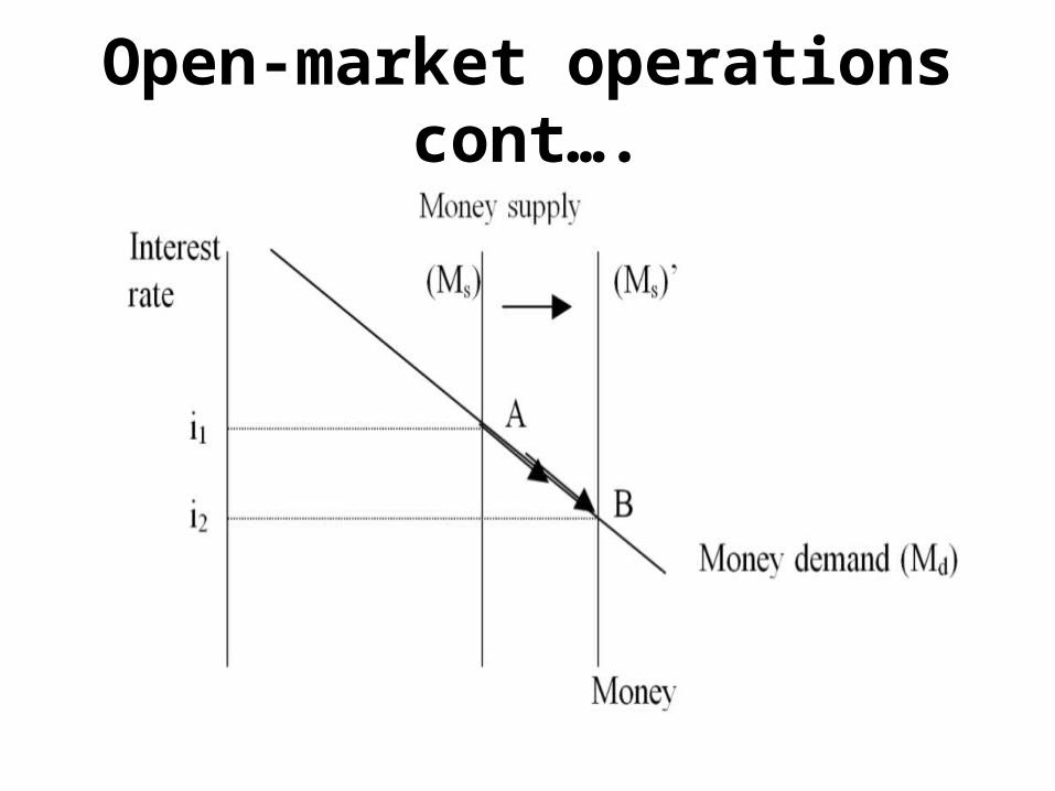
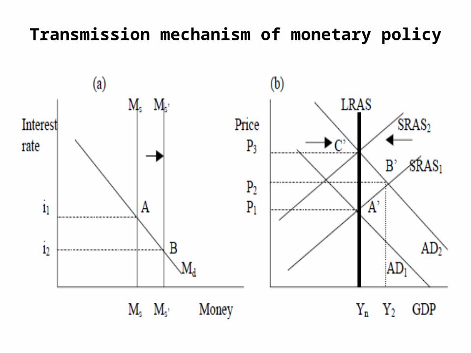
• Assume the central bank conducts an open-market operation in which it buys government bonds from the public (including the banks). This increases the money supply and lowers the interest rate. This is shown by a rightward shift in the Mscurve to Ms and an adjustment in the interest rate to i2, panel (a).
Transmission mechanism of monetary policy
• The lower interest rate stimulates investment as consumers, enjoying a lower cost of borrowing, buy more and larger houses and firms spend more on new machinery and equipment, and so on. As a result, the quantity of output demanded, at the given price level, increases and the AD curve shifts to the right to AD2, panel (b).
Transmission mechanism of monetary policy
• The short-run impact of this expansionary monetary policy is an increase in the level of output, represented by Y2, and a surge in price, P2. Of course, this adjustment entails subsequent changes in price and output beyond the short run. At the next stage, SRAS1 begins to shift to the left, reflecting an upward pressure on nominal wages. In the long run, the economy reverts to LRAS, settling at Point C’, where AD crosses LRAS.
Transmission mechanism of monetary policy
Transmission mechanism of monetary policy
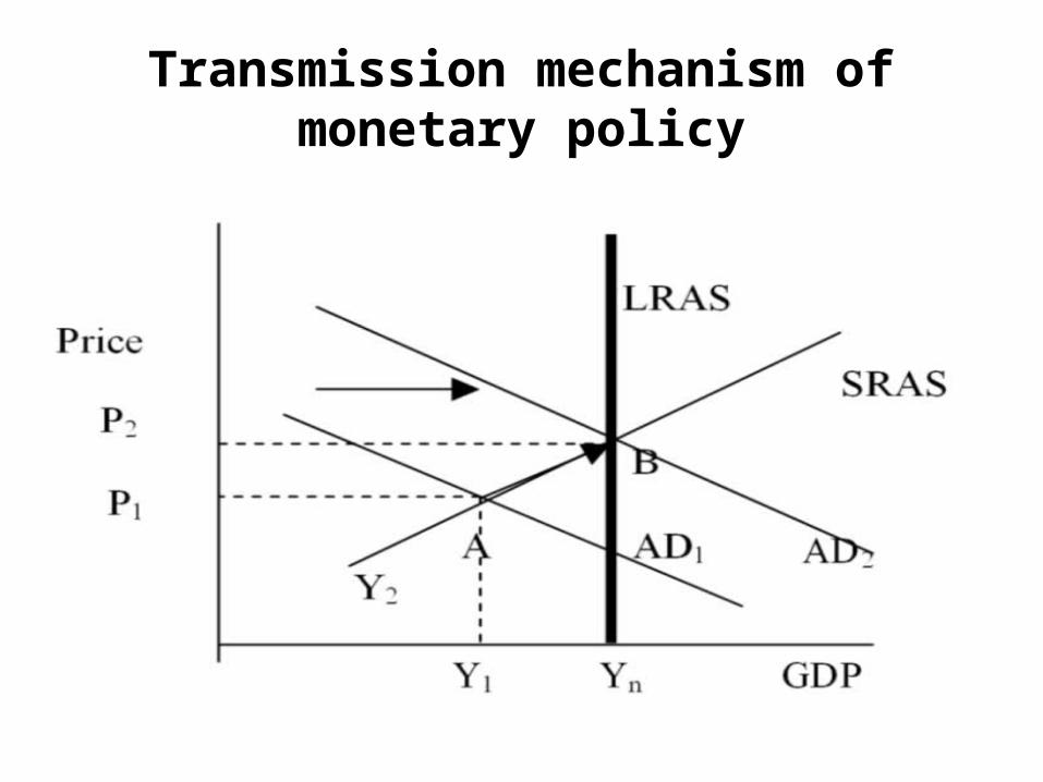
• The figure above illustrates a policy appropriate to the above analysis but in a situation where the economy starts from a recessionary gap instead, (Y1 –Yn) <0. An expansionary monetary policy could be designed to shift the aggregate demand curve by exactly the right amount to cross the SRAS along LRAS curve, point B. This would be the final (long-run) equilibrium situation where the economy will settle in.
Transmission mechanism of monetary policy
• How much extra aggregate demand is needed?• To be effective, the expansionary (counter-cyclical)
monetary policy, requires accurate information on the current level of GDP (Y1) and on the gap between it and potential GDP, (Y1 - Yn). Identifying the size of the gap, however, involves painstaking research and good judgement. It can be a hazardous exercise. A thorough and accurate job requires large econometric models of the economy comprising many equations to estimate these curves and their parameters first.
Objectives of monetary policy
• Central banks around world have shifted their focus to price stability as their main objective. Price stability is defined as the sustained absence of both inflation (prices rising too fast) and deflation (falling prices).
Ingredients of a successful price stability programme
• It requires political commitment. • An informed public opinion is also important.• Central banks should be largely independent
of political control. • Central banks also need a clear statement of
their policy objective.
Budget deficits, debts and fiscal policy
• Governments can affect spending and output levels in an economy through two sets of instruments;
• monetary policy. However, governments can have an extensive impact on the economy through taxation and government purchases.
• Such a policy is called fiscal policy –fiscal meaning budgetary.
Budget deficits, debts and fiscal policy cont….
• During a recession, governments increase spending and output in an economy-expansionary fiscal policy. Such a policy involves increasing government purchases, decreasing taxes or both.
• During an inflationary boom, the concentration is geared towards restraining spending and output –contractionary fiscal policy, which involves decreasing government spending and increasing taxes.
Discretionary versus automatic policy
• Because it is up to a government’s discretion to take these actions, fiscal policy is known as discretionary policy.
• In contrast, some stabilising forces are automatic. That is, they do not involve the direct involvement of government decision-makers.
The multiplier effect
• The multiplier effect is the magnified impact of any spending change on aggregate demand. It is the change in spending multiplied by a certain value to give the resulting change in aggregate demand.
The multiplier effect
• The spending multiplier is the value by which the initial spending change is multiplied by to give the total change in output –that is, the shift in the aggregate demand curve. This multiplier effect continues even after this first round and definitely does not stop at the third round. Once all these effects –a process that continues until the last-round effect is negligible –are added together, the total impact on the quantity of goods and services demanded can be much larger than the initial impulse from higher government spending.
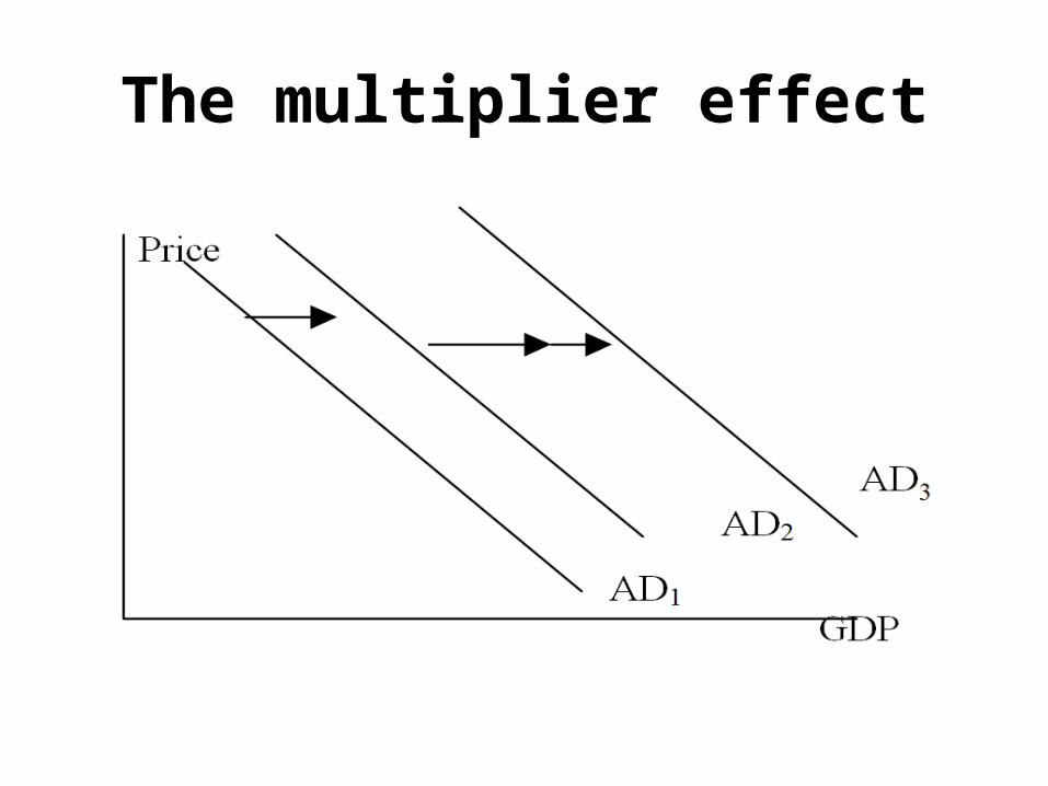
The multiplier effect
• The figure below illustrates the multiplier effect. The increase in government spending of $50 billion initially shifts the aggregate-demand curve to the right from AD1 to AD2 by exactly $50 billion. But when consumers respond by increasing their spending, the aggregate-demand curve shifts further to AD3.
The multiplier effect
The multiplier effect
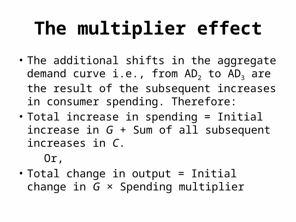
• The additional shifts in the aggregate demand curve i.e., from AD2 to AD3 are the result of the subsequent increases in consumer spending. Therefore:
• Total increase in spending = Initial increase in G + Sum of all subsequent increases in C.
Or,• Total change in output = Initial change in G ×
Spending multiplier
The multiplier effect
• For a given initial increase in G, the bigger the second term on the right, the bigger the overall effect on output (the left-hand side) and the greater the multiplier. Since the size of the change in C (second term on the right) is determined by MPC, we can conclude that the bigger MPC, the greater the impact of fiscal policy on the economy. Put differently, the smaller the marginal propensity to save (withdrawal), the larger the multiplier.
The multiplier effect
• Mathematics helps determine the magnitude of the spending multiplier in this case, which incorporates the initial as well as the subsequent effects on GDP:
• Multiplier = change in GDP/ change in G = 1/(1-MPC).
A successful expansionary fiscal policy
• An expansionary fiscal policy or fiscal stimulus is designed to increase aggregate demand by increasing government expenditure or transfer payments, or decreasing in taxes (or combination of all three actions) to eliminate a recessionary gap. The initial increase in aggregate demand from the cut in taxes or hike in transfer payments or government expenditure is reinforced by the multiplier effect. The aggregate demand curve (AD) shifts rightward from AD0 to AD1.
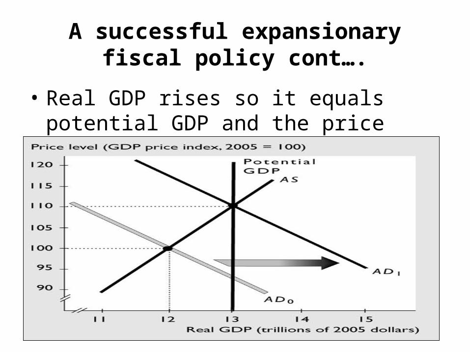
A successful expansionary fiscal policy cont….
• Real GDP rises so it equals potential GDP and the price level increases.
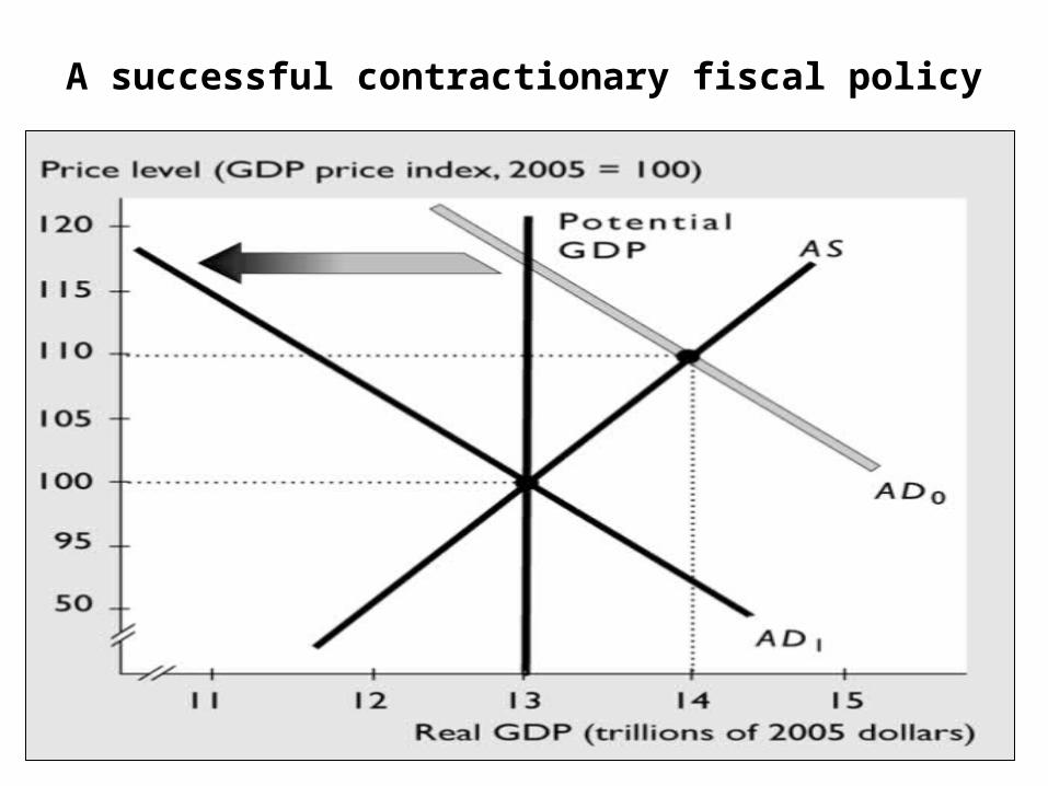
A successful contractionary fiscal policy
Effect of a tax cut
• Lower taxes leave households and businesses with more funds to spend and invest. In this case, the initial spending stimulus of the tax cut is multiplied by the spending multiplier, or the reciprocal of MPS, which is also equal to (1/(1-MPC). The result is an increase in total output, shown as a shift in the aggregate demand curve.
Effect of a tax cut
• The effect of a tax change can be summarised in mathematical terms similar to those which show the effect of a change in government spending.
• Total change in output = Initial change in spending × Spending multiplier
• -(MPC × change in T) × (1/ (1−MPC))
The crowding-out effect on investment
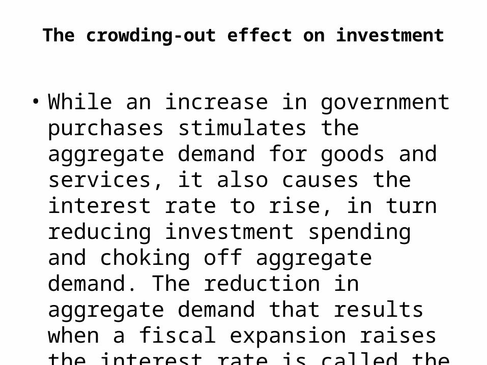
• While an increase in government purchases stimulates the aggregate demand for goods and services, it also causes the interest rate to rise, in turn reducing investment spending and choking off aggregate demand. The reduction in aggregate demand that results when a fiscal expansion raises the interest rate is called the crowding-out effect on investment.
The crowding-out effect on investment
The crowding-out effect on investment
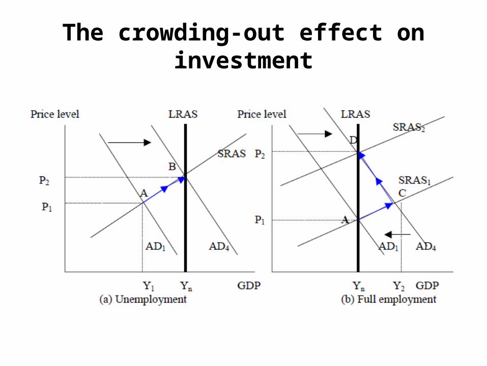
• An increase in government spending shifts the AD curve from AD1 to AD4. This shift is a net of three effects.
• The initial impact of G,• the subsequent impacts on C, through the
marginal propensity to consume (the multiplier effect), and
• the crowding-out effect on investment.
The crowding-out effect on investment
• The first two effects tend to reinforce each other, pushing the AD curve to the right, whereas the third effect tends to work in the opposite direction, pushing the AD curve to the left.
Government budgets
• The government’s budget balance is equal to its revenues minus its outlays. That is,
• Budget balance = Revenues – Outlays,• where outlays consist of expenditures on
goods and services (G), transfer payments such as welfare benefits, and debt interest charges, which are payments of interest on previously accumulated debt.
Government budgets
• When revenues exceed outlays, the government has a budget surplus. If outlays exceed revenues, the government has a budget deficit. If revenues equal outlays, the government has a balanced budget.
Deficits and debts
• The government borrows to finance its deficit. Government (public) debt is the total amount of government borrowing. It is the sum of past deficits minus the sum of past surpluses. When the government has a deficit, its debt increases.
• Debt (in 2002) = Debt (in 2001) + Deficit or surplus (in 2002)
Differences in the structure of the lags in fiscal versus monetary policy.
• Monetary and fiscal policy have differential impacts on aggregate demand; fiscal policy, at least a change in government spending, affects aggregate demand directly whereas monetary policy has an indirect effect on it. As such, fiscal policy tends to have a shorter execution lag.
Differences in the structure of the lags in fiscal versus monetary policy.
• Monetary policy lags are substantially shorter from the perspective of implementation, implementation lag. Implementation lags in fiscal policy are largely attributable to the political process. A fiscal policy typically requires an Act of parliament, budgetary preparation and presentation before the policy takes effect, whereas monetary policy does not. Therefore, while the overall length of the policy lags may be similar in both policies, the composition of them is different.
Inflation and Unemployment
• Inflation, is a general increase in the prices of goods and services in the entire economy over time.
• One key price index is the Consumer Price Index (CPI). The CPI is the tool most commonly used to measure overall changes in price in a representative basket of consumer products. Another important price index is the GDP deflator–a broader measure of average price. This index is found by dividing the nominal value of GDP by the real GDP.
Inflation and Unemployment
• To measure inflation rate, we calculate the annual percentage change in the price level. For example, the rate of inflation in year 2002 is calculated as follows:
• Inflation rate(2002) = CPI2002 – CPI2001×100
CPI2001
• . If the price level is rising, the inflation rate is positive. If the price level rises at a faster rate, the inflation rate will rise. In addition, the higher the new price level is, the lower the value of money and the higher the inflation rate.
Causes of inflation
• Demand-pull inflation• An inflation that results from an initial increase
in aggregate demand is called demand-pull inflation.
• An increase in the money supply.• An increase in government expenditures.• Increases in exports.• An increase in consumers’ and investors’
willingness to buy.
Inflation
Inflation
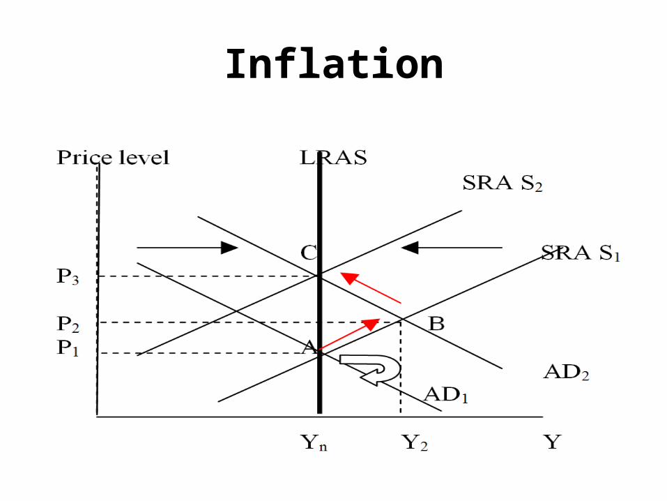
• Of course, this is not the end of the process of the adjustment. The reason is that GDP cannot remain above its potential value forever. Furthermore, with unemployment below its natural rate, there will be a shortage of labour. In this situation, the money wage rate begins to rise. As it does, short-run aggregate supply decreases and the SRAS1 curve starts to shift leftward.
Inflation
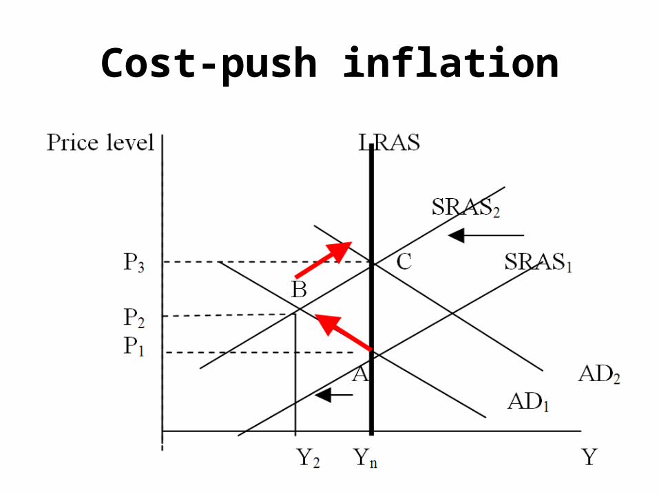
• The price level rises further and real GDP begins to decrease. With no further change in aggregate demand –the aggregate demand curve remains at AD – this process ends when the short-run aggregate supply curve has shifted to SRAS2. At this time, the price level has increased to P3 and real GDP has returned to potential GDP of Yn, the level from which it started.
Cost-push inflation
• An inflation that results from an initial increase in costs is called cost-push inflation. The two main sources of increases in costs are an increase in the money wage rate and an increase in the price of raw materials.
Cost-push inflation
Money supply and inflation
If each of us woke up today with twice as much money as yesterday, two things could happen:
• We could spend some of the extra money on goods and services to celebrate our good fortune, which would cause the price level to rise, or
• We might invest part of the money in government bonds or similar financial assets. In this case also, the resultant surge in asset prices would confer upon the public a positive wealth effect that would in turn boost demand for goods and services. Hence, prices would be driven up –assuming fixed production.
Money supply and inflation
• Ultimately, if the level of output remained unchanged despite this surge in demand, prices would be rising to the same extent as the nominal supply (stock) of money –doubled –and the initial equilibrium would be restored with prices and the nominal income being twice as much as they were originally.
Money supply and inflation
• In this situation, people are willing to hold all the 100 per cent increased supply of money because the real purchasing power of the public has remained unchanged despite the doubling of the money supply. Now, one needs to hold twice as much money as before, since the price of everything has doubled. This explains why inflation cannot continue without a sustained increase in the money stock and why continued excessive increases in the money stock are invariably followed by inflation.
Money supply and inflation
• The long-term impact of the increase in the money supply may be different from its short-run impact.
• In the short run, a rise in the money stock causes higher prices, but it also leads to more output. The output effect occurs because of short-term rigidities, reflecting employees’ inability to respond instantaneously to the decrease in the real wage caused by the increase in the price level. In the longer term, pay levels catch up on inflation and, over time, they will respond more quickly to it. The economy then approximates more and more closely to the vertical aggregate supply.
The Quantity Theory of Money.
• Ms.V = P.Y
• Where Ms = the money supply; V the velocity of circulation of money (the number of times money changes hands); Y = the real GDP; and P = the general price level.
• The equation holds that the nominal GDP (P.Y) is determined by the quantity of money in circulation and by the velocity of the money.
The Quantity Theory of Money.
• For a given velocity, the equation suggests that as the central bank increases the quantity of money in circulation, the nominal GDP on the right-hand side increases. Assuming that in the long run, the economy is at its full employment level of GDP (Y = Yn) and that full employment of GDP is constant, a direct link is established between changes in Ms and changes in P. An increase in Ms results in an increase in P of equal proportions –one for one.
The Quantity Theory of Money.
• This can also be expressed in percentage terms. Other things being equal (notably, the velocity of circulation and trend growth in income), the higher the growth of money supply, the higher the rate of inflation. Hence, the popular description of inflation is too much money chasing too few goods.
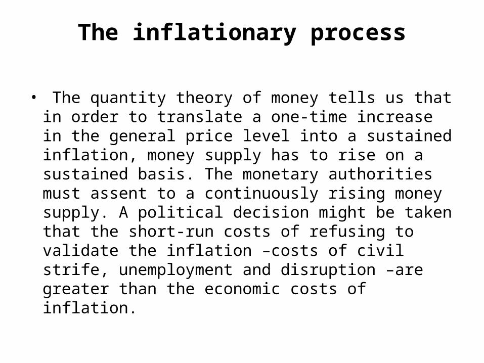
The inflationary process
• The quantity theory of money tells us that in order to translate a one-time increase in the general price level into a sustained inflation, money supply has to rise on a sustained basis. The monetary authorities must assent to a continuously rising money supply. A political decision might be taken that the short-run costs of refusing to validate the inflation –costs of civil strife, unemployment and disruption –are greater than the economic costs of inflation.
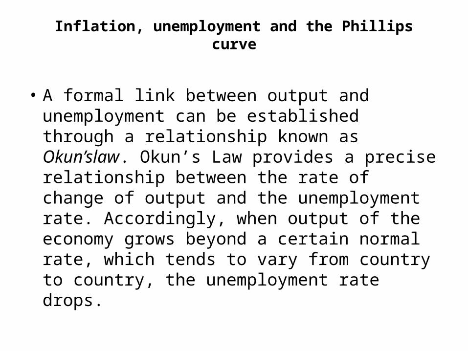
Inflation, unemployment and the Phillips curve
• A formal link between output and unemployment can be established through a relationship known as Okun’slaw. Okun’s Law provides a precise relationship between the rate of change of output and the unemployment rate. Accordingly, when output of the economy grows beyond a certain normal rate, which tends to vary from country to country, the unemployment rate drops.
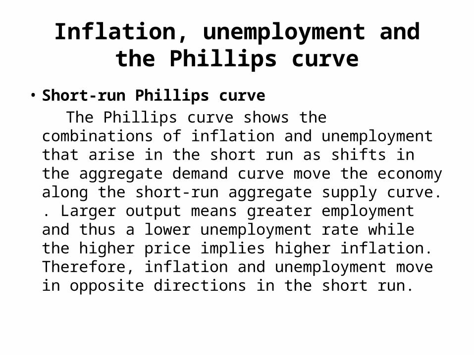
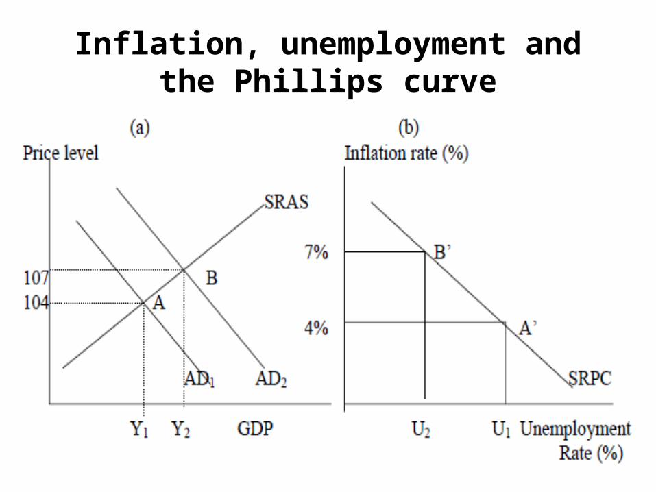
Inflation, unemployment and the Phillips curve
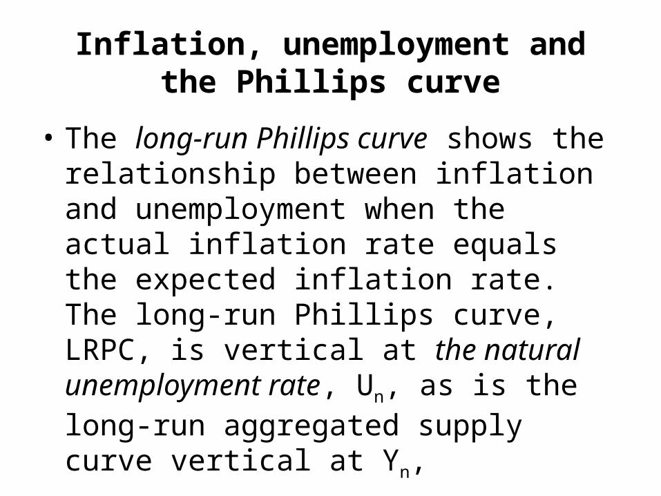
• Short-run Phillips curve The Phillips curve shows the combinations of
inflation and unemployment that arise in the short run as shifts in the aggregate demand curve move the economy along the short-run aggregate supply curve. . Larger output means greater employment and thus a lower unemployment rate while the higher price implies higher inflation. Therefore, inflation and unemployment move in opposite directions in the short run.
Inflation, unemployment and the Phillips curve
Inflation, unemployment and the Phillips curve
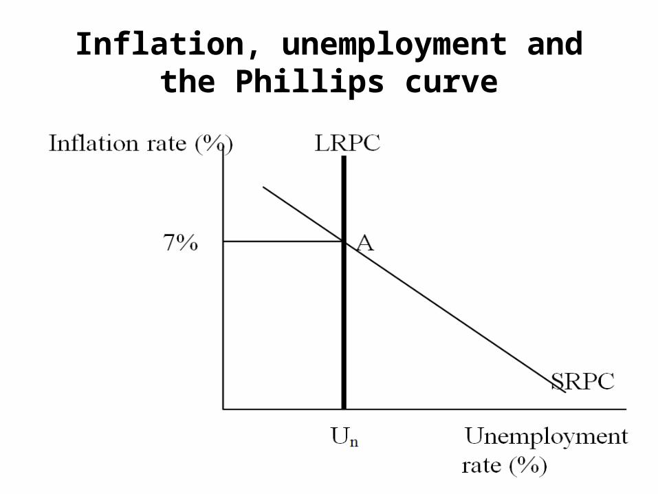
• The long-run Phillips curve shows the relationship between inflation and unemployment when the actual inflation rate equals the expected inflation rate. The long-run Phillips curve, LRPC, is vertical at the natural unemployment rate, Un, as is the long-run aggregated supply curve vertical at Yn,
Inflation, unemployment and the Phillips curve
Inflation, unemployment and the Phillips curve
• Consequently, the relationship between LRPC and SRPC is the mirror image of that between LRAS and SRAS. The long-run aggregate supply curve told us that any anticipated price was possible at the natural level of output: actual GDP equals potential GDP. In the same way, the long-run Phillips curve tells us that any anticipated inflation rate is possible at the natural unemployment rate.
Inflation, unemployment and the Phillips curve
• When the expected price level changes, the short-run aggregate supply curve shifts upward, but the long-run aggregate supply curve does not shift. Similarly, when the expected inflation rate changes, the short-run Phillips curve shifts up, but the long-run Phillips curve does not shift.
Costs of inflation
• If a household’s nominal income increases steadily every year but inflation is at a higher rate, the household suffers from losses of purchasing power. If, in contrast, the same household has a nominal income that increases at roughly the same rate as inflation, the household maintains its purchasing power.
Costs of inflation
• The damaging aspect of inflation for society is that it redistributes (income) wealth among individuals in an arbitrary way. The winners are often those with substantial economic resources, while the losers are usually those least able to withstand a drop in purchasing power.
Costs of inflation
• Shoe-leather costs• Increases in the inflation rate cause increases in the
nominal interest rate. Faced by this increase in the opportunity cost of money, individuals reduce their holdings of real money balances to economise on holding cash. Cash is, of course, subject to a greater deterioration than alternative assets that at least provide some kind of monetary return. Individuals, still in need of cash to finance their regular transactions but hold less money, must make more trips to the bank. These trips reduce leisure and/or time spent working, and are referred to as shoe-leather costs.
Tax distortions
• Increases in inflation can increase the effective tax rate on consumers through a process called bracket creep by pushing them into higher income-tax brackets as their nominal income increases.
Confusion and money illusion
• As inflation increases, decision making becomes more challenging, and certain computations become more difficult. Higher inflation tends to mask the real earnings of individuals.
Inflation variability
• Another problem with inflation is that often, as inflation rises, it becomes more variable too. It is the variability that makes lending and borrowing more risky. One implication is that bond holding becomes riskier.
Inflation tax
• When the government raises revenue by printing money, it is said to levy an inflation tax. The inflation tax is not exactly like other taxes, however, because no one receives a bill from the government for this tax.
Unemployment
The labour force is made up of those who either have jobs or are actively seeking employment. By its definition, the labour force leaves out those who have given up looking for a job, as well as full-time homemakers who, while they work, do not do so in the formal job market.
The official unemployment rate
• A person is unemployed if he or she is on temporary layoff looking for a job, or is waiting for the start date of a new job.
• Labour force= Number employed + Number unemployment
• Unemployment rate (%)• = Number of unemployed ×100 Labour force
The official unemployment rate
• The participation rate measures the percentage of the total adult population that makes up the labour force.
• Participation rate (%) = Labour force x 100 Adult population
Drawbacks of the official unemployment rate
• Underemployment• Discouraged workers- Discouraged workers
are those who, after a period of searching for a job unsuccessfully, have given up looking.
Anatomy of unemployment
• Large variations in unemployment rates across age groups.• Large variations in unemployment rates across regions in
large and diversified countries, especially those subject to disparate impacts in different regions.
• Each month, substantial movement of individuals in and out of unemployment –either to employment or out of the labour force, most of those who have become unemployed in any given month remaining unemployed for only a short period of time.
• Much of the unemployment rate representing people who will be unemployed for a long period of time.
The unemployment pool
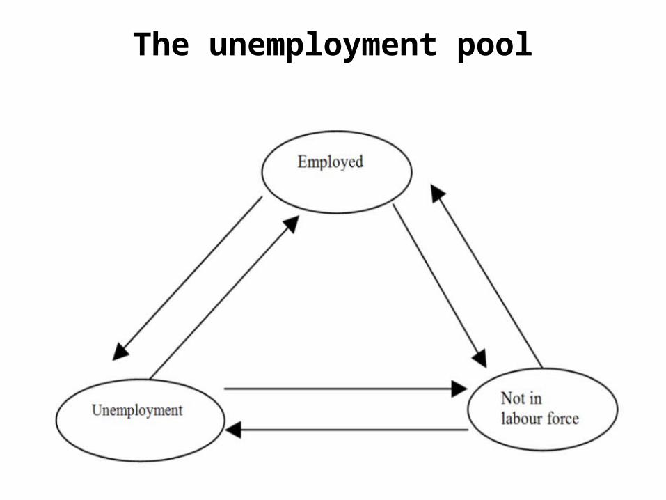
• Any time there is a given number or pool of unemployed people, there are flows in and out of the unemployment pool.
• Workers may become unemployed for one of the following reasons:
• Loss of a job through dismissal, layoff or closing down of a firm, followed by searching for another job. A layoff means that the worker was not fired and will return to the old job if demand for the firm’s product recovers.
• Quitting a workplace and searching for another job.• Entering or re-entering the labour force to search for a job.
The unemployment pool
• Individuals may end a spell of unemployment if they:
• Are hired or (in the case of laid-off persons) recalled.
• Withdraw from the labour force by stop looking for a job and thus, by definition, leave the labour force.
The unemployment pool
Types of unemployment
• Frictional unemployment• Workers who are temporarily between jobs or have begun
looking for their first jobs are experiencing frictional unemployment.
• Structural unemployment• Structural unemployment is due to a mismatch between
people and jobs. Unemployed workers cannot fill the jobs that are available. This type of unemployment occurs primarily because of changes in technology and the phenomenon of globalisation that tend to introduce sectoral shifts and workplace demands for new required skills. distance may be responsible for this type of unemployment:
Types of unemployment
• Cyclical unemployment Cyclical unemployment is primarily caused by
fluctuations in spending; it is demand- driven.• Seasonal unemployment In some industries agriculture, fishing, construction,
and tourism, for example –work is seasonal, with unemployment rising during winter months and some workers becoming seasonally unemployed during spring and summer.
Full employment
• Full employment is the highest reasonable expectation of employment for the economy as a whole –a natural unemployment rate. Natural rate of unemployment consists of frictional and structural unemployment but traditionally excludes cyclical unemployment. This rate also excludes seasonal unemployment, which is already omitted from the official unemployment rate.
Determinants of the natural rate
• The organisation of the labour market, including the presence or absence of employment agencies, youth employment services and the like.
• The demographic makeup of the labour force: e.g., the increase in the number of households with two paid workers or a change in the birth rate or migration.
• The availability of unemployment compensation that tends to affect the ability and desire of the unemployed to keep looking for a better job.
• The pace and the direction of technological changes.• Minimum wage laws that affect the employability of teenagers
and workers with few employable skills.
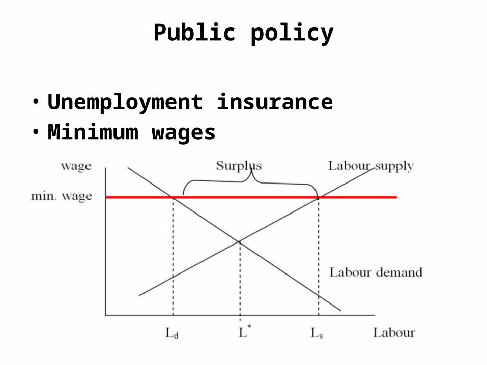
Public policy
• Unemployment insurance• Minimum wages
Public policy
• Minimum-wage laws are just one reason why wages may be too high. There are two other reasons why wages may be kept above the equilibrium level:
• Unions and collective bargaining. • Reservation wage and efficiency wage reservation wage is the wage at which accepting a
job offer has as much appeal to workers as rejecting it to stay unemployed and prolong their job search period.
Public policy
• Efficiency wage is the level above the reservation wage that firms pay workers in order to:
• increase the chances that productive workers will stay with the firm, and
• increase the cost to workers of losing their jobs if they are found shirking.
Costs of unemployment
• As individuals, unemployed people suffer both from their income loss and from the related social problems that long periods of unemployment cause. Society on the whole loses from unemployment because output is driven below its potential level.
Adjustment pattern of labour use during a recession
• Employers first adjust hours per worker –for example, by cutting overtime –and only trim their workforce.
• Layoffs and firings increase, increasing the flow into unemployment. However, at the same time, quits decrease as workers decide to hold on to their current job.
• It is possible that during a prolonged recession, many of the unemployed become discouraged and leave the labour force, making the official unemployment rate lower than it would otherwise be. As a result of all these effects, unemployment changes usually lag behind output changes.