Embed Size (px)
Citation preview

Motivation Model Calibration Results Appendix
Inequalities in an OLG economywith heterogeneous cohorts and pension systems
(with Joanna Tyrowicz, Krzysztof Makarski and Marcin Waniek)
Marcin Bielecki
Faculty of Economics, University of Warsaw
4th NBP Summer Workshop22-24 June 2015
1 / 33

Motivation Model Calibration Results Appendix
Motivation
Consumption inequality increases due to:Demographic transitionPension reform: defined benefit → defined contribution
Effects for wealth inequality: unclear
Can policy instruments help?minimum pensions: pensions ↑, labor supply incentives ↓contribution caps: mandatory savings replaced with private
Intuition insufficient – need quantitative answers
2 / 33

Motivation Model Calibration Results Appendix
Literature review
Distributional effects of pension systems: OLG models withex post heterogeneity:
Castaneda et al. (2003, JPE); Fehr et al. (2008, RED); Song(2011, RED); Bucciol (2011, MD); Cremer and Pestieau (2011,EER); Kumru and Thanopoulos (2011, JPubE); Fehr and Uhde(2014, EM); St-Amant and Garon (2014, ITPF)
Ex ante + ex post heterogeneity: education affects mortality ratesHairault and Langot (2008, JEDC):McGrattan and Prescott (2014, NBER)Kindermann and Krueger (2014, NBER)
3 / 33

Motivation Model Calibration Results Appendix
Our approach
Question 1: distributional effects of a pension system reform
Question 2: are standard instruments effective in reducingthe increase in inequality
Ex ante heterogeneous agents: age + within cohort
endowments + preferences ← not a standisolate the role of each separatelymost countries: no data on mortality by educationor income groups
4 / 33

Motivation Model Calibration Results Appendix
Results preview
DB→DC reform: consumption inequalities ↑, wealth inequalities ↓
Demographic transition: consumption inequalities ↑– effect larger than reform
Minimum pensions:reduce consumption inequality from the reform by approx. 40%work on the endowments margin, but not on preferences
Effects of the contribution cap: unnoticeable
5 / 33

Motivation Model Calibration Results Appendix
Results preview
DB→DC reform: consumption inequalities ↑, wealth inequalities ↓Demographic transition: consumption inequalities ↑– effect larger than reform
Minimum pensions:reduce consumption inequality from the reform by approx. 40%work on the endowments margin, but not on preferences
Effects of the contribution cap: unnoticeable
5 / 33

Motivation Model Calibration Results Appendix
Method
Modeldeterministic general equilibriumoverlapping generationsex ante heterogeneity: endowments + preferences
Calibrate to Poland in 1999
6 / 33

Motivation Model Calibration Results Appendix
Households I
“Born” at age 20 (j = 1) and live up to 100 years (J = 80)Subject to time and cohort dependent survival probability πBelong to a type k:
productivity level ωtime discounting δrelative leisure preference φ
Choose labor supply l endogenously until retirementMaximize remaining lifetime utility derived from consumption cand leisure 1− l:
Uj,k,t =J−j∑s=0
[δskπj+s,t+sπj,t
[cφkj+s,k,t+s (1− lj+s,k,t+s)1−φk
]]
7 / 33

Motivation Model Calibration Results Appendix
Households II
Subject to the budget constraint
(1 + τ ct )cj,k,t + sj,k,t = (1− τ lt )(1− τ)wtωklj,k,t ← labor income+ (1 + (1− τkt )rt)sj−1,k,t−1 ← capital income+ (1− τ lt )bj,k,t ← pension income+ beqj,k,t ← bequests−Υt ← lump-sum tax
There exists a closed-form solution to this problem
8 / 33

Motivation Model Calibration Results Appendix
Producers
Perfectly competitive representative firmStandard Cobb-Douglas production function
Yt = Kαt (ztLt)1−α
Profit maximization implies
wt = zt(1− α)kαtrt = αkα−1
t − d
9 / 33

Motivation Model Calibration Results Appendix
Government
Spends a fixed share of GDP g on government consumptionCollects taxes TCloses the gap between pension system contributions and benefitsCan take on debt D
Tt +Dt = (1 + rt)Dt−1 + gYt + subsidyt
We fix debt at constant 45% debt to GDP ratio.Consumption tax varies to satisfy the government constraint.
10 / 33

Motivation Model Calibration Results Appendix
Pension system
Pay As You Go Defined Benefit (PAYG DB)
bJ ,k,t = ρ · gross wageJ−1,k,t−1
Pay As You Go Defined Contribution (PAYG DC)
bJ ,k,t =accumulated sum of contributionsJ ,k,t
expected remaining lifetimeJ ,t
Pensions indexed by the rate of annual payroll growth
11 / 33

Motivation Model Calibration Results Appendix
Instrument 1: minimum pensions
Definitionbj,k,t ≥ ρmin · gross average waget
We set ρmin = 0.2 → 4% coverage (consistent with the data)
Expected effectsAffects directly only the left tail of income distributionIncreases lifetime incomes of targeted group: consumptioninequality should decreaseLower incentives for private savings: possible increasein consumptionLower incentives to work: possible reduction in hours worked
12 / 33

Motivation Model Calibration Results Appendix
Instrument 2: contribution cap
Definition:
τ effj,k,t = min
τ,τcap · gross average waget
wtωklj,k,t
To replicate 2% coverage, τcap = 1.7 (lower than de iure 2.5)
Expected effectsAffects directly only the right tail of income distributionLower contributions of targeted group: higher voluntary saving rates→ wealth inequalities ↑, capital accumulation ↑Matters because market interest rates and social security indexationdiffer
13 / 33

Motivation Model Calibration Results Appendix
Solution procedure
Gauss-Seidel iterative algorithmSteady states (initial and final)
1 Guess an initial value for k2 Use it to compute the prices3 Have households solve their problem given prices4 Aggregate individual labor supply and savings to get new values
for L and K5 If the new value for k satisfies predefined norm, finish,
else update k and return to point (2)Transition path
1 Basing on the initial and final steady state values for k guess aninitial path between the terminal points...
14 / 33

Motivation Model Calibration Results Appendix
Exogenous assumptions
Projections for Poland provided by the European Commission
Population Size TFP Growth
Kept constant across scenarios, don’t affect results
15 / 33

Motivation Model Calibration Results Appendix
Exogenous assumptions
Projections for Poland provided by the European Commission
Population Size TFP Growth
Kept constant across scenarios, don’t affect results
15 / 33

Motivation Model Calibration Results Appendix
Within cohort heterogeneity: endowments
Structure of Earnings Survey, 1998, Poland
Productivity ω
Resulting: 10 values for ω
16 / 33
Motivation Model Calibration Results Appendix
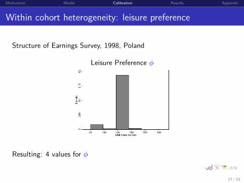
Within cohort heterogeneity: leisure preference
Structure of Earnings Survey, 1998, Poland
Leisure Preference φ
Resulting: 4 values for φ
17 / 33

Motivation Model Calibration Results Appendix
Within cohort heterogeneity: time preference
Again: no data on mortality rates or wealth by incomeor education groups
Calibrate the central value of δ to match the interest rateSplit population ad hoc to 3 groups:
discount factors are (0.98δ, δ, 1.02δ)
18 / 33

Motivation Model Calibration Results Appendix
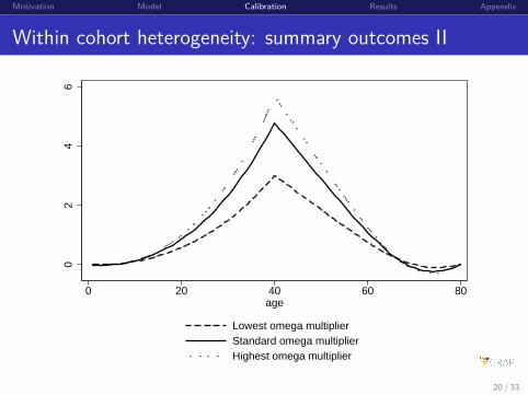
Within cohort heterogeneity: summary outcomes I
Productivity values and leisure preference parameters matchedto replicate dataDiscount factors differentiated ad hocIn total we have 120 types within each cohort
The resulting consumption Gini index in the initial steady stateis 25.5, consistent with Brzezinski (2011)
19 / 33
Motivation Model Calibration Results Appendix
Within cohort heterogeneity: summary outcomes II0
24
6
0 20 40 60 80age
Lowest omega multiplierStandard omega multiplierHighest omega multiplier
20 / 33

Motivation Model Calibration Results Appendix
Within cohort heterogeneity: summary outcomes III−
50
510
0 20 40 60 80age
Lowest delta multiplierHighest delta multiplierStandard multipliersLowest phi multiplierHighest phi multiplier
21 / 33

Motivation Model Calibration Results Appendix
Minimum pensions coverage (demographic transition)0
.2.4
.6.8
1
2000 2050 2100 2150 2200 2250year
Defined Benefit with minimum pensionsDefined Contribution with minimum pensions
22 / 33

Motivation Model Calibration Results Appendix
Consumption Gini.2
4.2
6.2
8.3
2000 2050 2100 2150 2200year
DB: No instrumentsDC: No instrumentsDC: Minimum benefits
23 / 33

Motivation Model Calibration Results Appendix
Wealth Gini.8
5.9
.95
11.
05
2000 2050 2100 2150 2200year
DB: No instrumentsDC: No instrumentsDC: Minimum benefits
24 / 33

Motivation Model Calibration Results Appendix
Inequality decomposition – endowments vs preferences
Clear arguments for reducing inequality stemmingfrom endowments (luck), not so much from preferencesTo isolate the effects of the two sources:
Shut down each channel separatelyKeep prices constant from the full model to avoid GE effectsSolve for decisions of households in partial equilibrium
25 / 33

Motivation Model Calibration Results Appendix
Consumption inequality decomposition
Fixed endowments Fixed preferencesDiffering preferences Differing endowments
.05
.1.1
5.2
.25
.3
2000 2050 2100 2150 2200year
DB: Fixed endowments, no instrumentsDC: Fixed endowments, no instrumentsDC: Fixed endowments, minimum benefits
.05
.1.1
5.2
.25
.3
2000 2050 2100 2150 2200year
DB: Fixed preferences, no instrumentsDC: Fixed preferences, no instrumentsDC: Fixed preferences, minimum benefits
26 / 33

Motivation Model Calibration Results Appendix
Wealth inequality decomposition
Fixed endowments Fixed preferencesDiffering preferences Differing endowments
0.2
.4.6
.81
2000 2050 2100 2150 2200year
DB: Fixed endowments, no instrumentsDC: Fixed endowments, no instrumentsDC: Fixed endowments, minimum benefits
0.2
.4.6
2000 2050 2100 2150 2200year
DB: Fixed preferences, no instrumentsDC: Fixed preferences, no instrumentsDC: Fixed preferences, minimum benefits
27 / 33

Motivation Model Calibration Results Appendix
Macroeconomic effects
No instrument Minimum pension Contribution capDB DC DB DC DB DC
Capital 52.6% 60.4% 52.7% 60.3% 52.6% 60.5%Consumption tax rate (τ c)
initial 11.00 11.00 11.00 11.00 11.00 11.00final 15.44 10.95 15.43 11.99 15.46 10.95
Pension system deficitinitial 1.46 1.56 1.46final 3.95 0.00 4.02 0.87 3.97 0.00
28 / 33

Motivation Model Calibration Results Appendix
Welfare effects
Defined Benefit Defined Contribution
−.0
004
−.0
002
0.0
002
Wei
ghte
d M
ean
Com
pens
atin
g V
aria
tion
2000 2050 2100 2150 2200 2250Year of birth
Minimum benefitsContributions cap
−.0
03−
.002
−.0
010
Wei
ghte
d M
ean
Com
pens
atin
g V
aria
tion
2000 2050 2100 2150 2200Year of birth
Minimum benefitsContributions cap
29 / 33

Motivation Model Calibration Results Appendix
Conclusions
Consumption inequalities increase due todemographic transitionDB → DC reform
Minimum pensionseffective in reducing consumption inequality resultingfrom the DB → DC reform by approx. 40%with 80% coverage minimum pension costs ∼ 1 pp higherconsumption tax (transfer of about 0.9% GDP)wealth inequality increases
Contribution cap has virtually no effects
30 / 33

Motivation Model Calibration Results Appendix
Thank you for your attention
31 / 33

Motivation Model Calibration Results Appendix
Household sector closed form solution IFor j < J (working):
cj,t = Ωj,t + Γj,t(1 + τ ct )
[∑J−j−1s=0
((1 + φ) δs πj+s,t+s
πj,t
)+∑J−js=J−j
(δsπj+s,t+s
πj,t
)]lj,t = 1− φ(1 + τ ct )cj,t
(1− τ lt )(1− τ)wtsj,t = (1− τ lt )(1− τ)wtlj,t + (1 + (1− τkt )rt)sj−1,t−1 − (1 + τ ct )cj,t,
with
Ωj,t =J−j−1∑s=0
(1− τ lt+s)(1− τ)wt+s + beqj+s,t+s −Υt+s∏si=1(1 + (1− τkt+i)rt+i)
Γj,t =J−j∑s=J−j
(1− τ lt+s)bj+s,t+s + beqj+s,t+s −Υt+s∏si=1(1 + (1− τkt+i)rt+i)
.
32 / 33

Motivation Model Calibration Results Appendix
Household sector closed form solution II
For j ≥ J (retired):
cj,t = Γj,t(1 + τ ct )
[∑J−js=J−j
(δsπj+s,t+s
πj,t
)]lj,t = 0sj,t = (1− τ lt )bιj,t + (1 + (1− τkt )rt)sj−1,t−1 − (1 + τ ct )cj,t,
with
Γj,t =J−j∑s=0
(1− τ lt+s)bj+s,t+s + beqj+s,t+s −Υt+s∏si=1(1 + (1− τkt+i)rt+i)
.
33 / 33