Oil schocks

Oil Price Shocks and Stock Markets

Daniel Canedo DonosoUniversidad Nacional de Yokohama

Oil Price Shocks and Stock Markets

Oil prices have an effect on the real economy, because they increase the production costs of enterprises and reduce disposable income that consumers have.

It can be expected that an increase in oil prices have a negative effect on the activity level of an economy and its securities markets.

Objective

To study the effect of changes in oil prices in the stock price index and industrial production.

Compare the effect of oil prices on the economy with the effect of the interest rate.

Determine if the stock markets have a symmetric response to positive and negative changes in oil prices.

Hypothesis

Oil prices affect an industrialized economy. Because it can affect the behavior of the share price index and the level of economic activity measured by the industrial production index.

Contribution

To study the effect of changes in oil prices in the stock indices of the three largest markets in the world.

The Standard and Poor's (U.S.), Nikkei225 (Japan) FTSE100 (UK). The data sample covers the period from January 1986 to August 2008.

Data

The sample period is in series month (January 1986 to August 2008)

The oil price series are; W.T.I. Europe Brent spot price and spot price. These data pertain to the Department of Energy of the United States..

Data

Interest rate on short term. Rate at 3 months treasury bills of the U.S. The rate of Japan collateral overnight. The discount rate 3-month treasury bills (monthly average) for the UK.

Federal Reserve, Bank of Japan and Bank of England. Interest rates are measured in real terms.

Data

The Industrial Production Index and the Consumer Price Index were obtained from the database of the OECD.

Both indices are seasonally adjusted and have as the base year 2000.

Data

All variables are transformed to logarithms for comparison.

The variable rsr (Real Stock Prices) is the difference between compound return - stock index log difference - and inflation - log difference of the consumer price index.

Oil prices are referred to as industrial production as lip and the interest rate as lr.

Econometric Analysis.

A VAR model is used to see the relationships between interest rates, oil prices, industrial production and stock indexes.

First, the properties of the time series are examined. Unit Root Test. Co- integration Test.


VAR model is executed. Variance Decomposition to period 24. Impulse Response Function.

VAR analysis period is divided into 2 sub periods. To see whether the effect of oil price changes between the sub

periods. To compare its effect with the effect of the rate.


Asymmetry of oil shocks. The sample is divided between positive changes and negative changes in oil prices. Wald Test. Variance Decomposition to period 24. Impulse Response Function.

The VAR sample period divided into two sub periods. To compare the changes in sensitivity to positive changes and negative

changes in oil prices.

U. S. Stock Market

The variance of the market is affected by changes in oil prices in the U.S. at 9.51%, UK 7.51%, and 4.4% in Japan.

The stock market and industrial production has increased despite higher oil prices.

U. S. Stock Market Graph 1; S&P500, WTI, Index of IP, 3 month T-Bill.

0

400

800

1,200

1,600

1990 1995 2000 2005

SP

0

2

4

6

8

10

1990 1995 2000 2005

R

0

20

40

60

80

100

120

140

1990 1995 2000 2005

WTI_SPOT

50

60

70

80

90

100

110

1990 1995 2000 2005

IIP

U. S. Stock MarketTable 1Unit Root Test; Phillips and Perron (1988)

1 : 1986 : 01 2008 : 08t t t ty y u t

Variable Adj. t-Stat ProbabilityIn levelslr -1.342472 0.6102lo 0.093775 0.9648lip -1.211734 0.6701rsr *** -16.03766 0.0000In first differencesdlr *** -10.37303 0.0000dlo *** -13.72265 0.0000dlip *** -15.47861 0.0000drsr *** -43.61414 0.0001

Notes. ***, ** and * denote if a test statistic is significant at the 1%, 5%, and 10%significance level, respectively. Critical values for the test statistics are from *MacKinnon(1996) one-sided p-values. The truncation lag parameter is set at 5 for the Bartlet Kernelcorrection for serial correlation.

U. S. Stock MarketTable 2Tests for co-integration using the Johansen procedure

1

1

, `

{ , , }

p

t t t t p t

t

x x x

x lr lo lip

Period 1986:1 to 2008:08, lag p=12 is chosen using likelihood ratio tests.

Eigenvalues 0.046348 0.019235 0.005322

The test statistics for r equal to the number of cointegrating vectors

Hypothesis None At most 1 At most 2Trace test 18.70373 6.412458 1.382001lambda max test 12.29127 5.030457 1.382001

Notes ***, **, * denotes rejection of the null hypothesis at the 1%, 5% and 10% level ofsignificance, respectively. Critical values are from MacKinnon-Haug-Michelis (1999) p-values.

U. S. Stock MarketTable 3Variance decomposition of forecast error after 24 months

Variance decomposition of forecast error variance after 24 monthsStep Shocks to

e( r ) e( o ) e( p ) e( rs )

Ordering (dlr, dlo, dlip, rsr), 1986:01 to 2008:08

dlr 84.27 4.09 6.38 5.26(6.39) (3.55) (4.26) (3.78)

dlo 3.17 88.75 3.79 4.29(4.82) (5.94) (2.86) (2.86)

dlip 7.87 9.51 80.11 2.51(4.80) (3.48) (5.61) (2.38)

rsr 8.50 7.42 10.96 73.12(4.66) (3.73) (4.50) (6.27)

Cholesky Ordering: dlr dlo dlip rsrStandard Errors: Monte Carlo (1000 repetitions)Monte Carlo constructed standard errors are shown in parentheses.

U. S. Stock MarketTable 4Variance decomposition of forecast error after 24 monthsVariance decomposition of forecast error variance after 24 monthsStep Shocks to

e( r ) e( o ) e( p ) e( rs )


dlr 70.13 11.27 11.68 6.92(10.98) (7.91) (7.87) (7.61)

dlo 5.66 78.13 8.98 7.23(6.94) (9.71) (7.99) (6.77)

dlip 9.22 14.03 61.67 15.08(7.61) (7.09) (9.48) (7.77)

rsr 9.21 11.12 9.06 70.61(6.33) (6.70) (5.97) (8.93)


dlr 73.17 5.45 4.15 17.22(10.43) (6.42) (5.90) (8.08)

dlo 23.25 59.10 6.50 11.15(10.69) (9.51) (5.36) (5.70)

dlip 24.41 5.27 58.96 11.36(10.19) (5.75) (9.16) (5.99)

rsr 18.37 13.52 14.23 53.88(10.14) (5.98) (5.87) (7.55)


U. S. Stock Market Graph 2; Impulse Response Function for 24 months

-.04

-.02

.00

.02

.04

.06

.08

5 10 15 20

Response of DLR to DLR

-.04

-.02

.00

.02

.04

.06

.08

5 10 15 20

Response of DLR to DLO

-.04

-.02

.00

.02

.04

.06

.08

5 10 15 20

Response of DLR to DLIP

-.04

-.02

.00

.02

.04

.06

.08

5 10 15 20

Response of DLR to RSR

-.04

.00

.04

.08

.12

5 10 15 20

Response of DLO to DLR

-.04

.00

.04

.08

.12

5 10 15 20

Response of DLO to DLO

-.04

.00

.04

.08

.12

5 10 15 20

Response of DLO to DLIP

-.04

.00

.04

.08

.12

5 10 15 20

Response of DLO to RSR

-.002

.000

.002

.004

.006

5 10 15 20

Response of DLIP to DLR

-.002

.000

.002

.004

.006

5 10 15 20

Response of DLIP to DLO

-.002

.000

.002

.004

.006

5 10 15 20

Response of DLIP to DLIP

-.002

.000

.002

.004

.006

5 10 15 20

Response of DLIP to RSR

-.02

.00

.02

.04

.06

5 10 15 20

Response of RSR to DLR

-.02

.00

.02

.04

.06

5 10 15 20

Response of RSR to DLO

-.02

.00

.02

.04

.06

5 10 15 20

Response of RSR to DLIP

-.02

.00

.02

.04

.06

5 10 15 20

Response of RSR to RSR

Response to Cholesky One S.D. Innovations ± 2 S.E.

U. S. Stock MarketTable 5 Oil price symmetry. Variance decomposition of forecast error after 24 months.Variance decomposition of forecast error variance after 24 monthsStep Shocks to

e( r ) e( o ) + e( o ) - e( p ) e( rs )Ordering (dlr, dlo+,dlo-, dlip, rsr), 1986:01 to 2008:08

dlr 82.67 6.61 4.38 9.73 8.19(6.87) (4.87) (4.49) (4.65) (4.64)

dlo + 3.76 79.39 23.12 6.65 5.10(3.33) (6.13) (4.46) (3.66) (2.84)

dlo - 1.61 4.90 63.99 3.95 9.12(3.10) (2.85) (5.84) (2.93) (3.52)

dlip 4.12 5.22 3.36 69.09 4.43(3.16) (2.75) (2.58) (5.78) (2.40)

rsr 7.84 3.88 5.15 10.57 73.16(4.44) (2.66) (2.90) (3.83) (5.50)


U. S. Stock MarketTable 6 Oil price symmetry .Variance decomposition of forecast error after 24 months.Variance decomposition of forecast error variance after 24 monthsStep Shocks to


dlr 68.46 3.88 9.44 9.08 9.20(11.33) (7.61) (7.76) (8.49) (7.02)

dlo + 8.35 61.64 24.83 15.14 6.47(8.17) (9.19) (7.75) (7.43) (6.65)

dlo - 5.79 9.62 42.84 6.27 16.99(6.95) (6.42) (7.56) (6.45) (6.88)

dlip 8.98 13.12 12.70 56.71 10.26(8.08) (7.70) (7.50) (9.60) (7.05)

rsr 8.43 11.75 10.19 12.80 57.08(7.61) (6.91) (6.65) (7.13) (8.14)

Ordering (dlr, dlo+,dlo-, dlip, rsr), 1996:12 to 2008:08

dlr 64.28 21.61 14.01 22.01 23.05(11.79) (9.63) (9.50) (9.71) (9.87)

dlo + 9.18 52.06 24.05 7.81 6.22(7.67) (8.26) (6.87) (6.61) (5.92)

dlo - 6.77 9.85 45.79 8.57 15.27(6.85) (5.94) (7.78) (5.90) (6.24)

dlip 4.50 9.25 6.80 51.50 14.33(5.68) (5.58) (5.25) (8.54) (5.97)

rsr 15.27 7.23 9.35 10.10 41.14(7.85) (5.34) (5.32) (6.06) (7.20)


U. S. Stock MarketTable 7Wald test of symmetry.

Wald Test:Test Statistic Value df Probability

F-statistic 0.131415 (1, 259) 0.717300Chi-square 0.131415 1.000000 0.717000Null Hypothesis Summary:Normalized Restriction (= 0)Value Std. Err.

C(4) + C(5) - C(6) - C(7) 0.047718 0.131632Restrictions are linear in coefficients.

4 5 6 7* (-1) + * (-2) * (-1)+ * (-2) =0dlopos dlopos dloneg dloneg

U. S. Stock Market Graph 3; Impulse Response Function for 24 months

-.04

-.02

.00

.02

.04

.06

.08

5 10 15 20


-.04

-.02

.00

.02

.04

.06

.08

5 10 15 20


-.04

-.02

.00

.02

.04

.06

.08

5 10 15 20


-.04

-.02

.00

.02

.04

.06

.08

5 10 15 20


-.04

.00

.04

.08

.12

5 10 15 20


-.04

.00

.04

.08

.12

5 10 15 20


-.04

.00

.04

.08

.12

5 10 15 20


-.04

.00

.04

.08

.12

5 10 15 20


-.002

.000

.002

.004

.006

5 10 15 20


-.002

.000

.002

.004

.006

5 10 15 20


-.002

.000

.002

.004

.006

5 10 15 20


-.002

.000

.002

.004

.006

5 10 15 20


-.02

.00

.02

.04

.06

5 10 15 20


-.02

.00

.02

.04

.06

5 10 15 20


-.02

.00

.02

.04

.06

5 10 15 20


-.02

.00

.02

.04

.06

5 10 15 20



U. K. Stock Market

The stock market of the UK showed some volatility. But it is important to note that the recovery of its stock market occurred during a hike in oil prices.

However, industrial production in the UK has been stagnant.

The following analysis desmuestra VAR that higher oil prices were bad for the industrial production in the UK but if pushed the stock market.

U. K. Stock Market Graph 4; FTSE100, Brent, Index of IP, 3 month T-Bill.

1,000

2,000

3,000

4,000

5,000

6,000

7,000

88 90 92 94 96 98 00 02 04 06 08

FTSE100

4

6

8

10

12

14

16

18

88 90 92 94 96 98 00 02 04 06 08

R

0

40

80

120

160

88 90 92 94 96 98 00 02 04 06 08

BRENT

80

85

90

95

100

105

88 90 92 94 96 98 00 02 04 06 08

IIP

U. K. Stock MarketTable 8Unit Root Test; Phillips and Perron (1988)

1 : 1987 : 06 2008 : 08t t t ty y u t Phillips and Perron (1988) Unit Root Tests.

Variable Adj. t-Stat ProbabilityIn levelslr -1.382751 0.5907lo 0.159564 0.9695lip -2.376197 0.1495rsr *** -15.39832 0.0000In first differencesdlr *** -11.05801 0.0000dlo *** -12.57271 0.0000dlip *** -22.66913 0.0000drsr *** -14.48577 0.0000


Phillips and Perron (1988) Unit Root Tests.Variable Adj. t-Stat Probability

In levelslr -1.382751 0.5907lo 0.159564 0.9695lip -2.376197 0.1495rsr *** -15.39832 0.0000In first differencesdlr *** -11.05801 0.0000dlo *** -12.57271 0.0000dlip *** -22.66913 0.0000drsr *** -14.48577 0.0000


U. K. Stock MarketTable 9Tests for co-integration using the Johansen procedure.

Tests for cointegration using the Johansen procedurePeriod 1986:1 to 2008:08, lag p=12 is chosen using likelihood ratio tests.

Eigenvalues 0.046825 0.014522 0.002416




1

1

, `

{ , , }

p

t t t t p t

t

x x x

x lr lo lip

U. K. Stock MarketTable 10Variance decomposition of forecast error after 24 months.Variance decomposition of forecast error variance after 24 monthsStep Shocks to

e( r ) e( o ) e( p ) e( rs )Ordering (dlr, dlo, dlip, rsr), 1987:06 to 2008:08

dlr 79.67 8.26 3.79 8.28(5.48) (4.04) (2.86) (3.60)

dlo 5.27 83.68 6.13 4.91(3.61) (5.37) (3.73) (3.19)

dlip 4.84 2.84 88.84 3.48(3.39) (2.91) (5.13) (2.87)

rsr 5.89 7.51 8.52 78.08(3.07) (3.39) (3.70) (5.18)


U. K. Stock MarketTable 11Variance decomposition of forecast error after 24 months.Variance decomposition of forecast error variance after 24 monthsStep Shocks to


dlr 54.04 19.35 10.43 16.17(9.94) (8.54) (7.72) (8.83)

dlo 19.11 57.56 9.95 13.39(9.94) (10.12) (8.22) (8.10)

dlip 13.59 8.42 60.52 17.47(8.87) (7.67) (10.41) (8.21)

rsr 12.39 9.78 11.10 66.73(7.90) (7.27) (7.88) (9.34)


dlr 74.49 8.14 7.89 9.48(10.02) (7.10) (8.03) (6.42)

dlo 7.50 78.27 7.40 6.84(5.64) (8.37) (5.92) (5.49)

dlip 7.04 6.62 82.33 4.01(5.75) (6.34) (8.63) (4.63)

rsr 7.74 15.37 14.01 62.88(6.02) (7.76) (6.30) (8.11)


U. K. Stock Market Graph 5; Impulse Response Function for 24 months.

-.02

.00

.02

.04

.06

5 10 15 20


-.02

.00

.02

.04

.06

5 10 15 20


-.02

.00

.02

.04

.06

5 10 15 20


-.02

.00

.02

.04

.06

5 10 15 20


-.04

.00

.04

.08

.12

5 10 15 20


-.04

.00

.04

.08

.12

5 10 15 20


-.04

.00

.04

.08

.12

5 10 15 20


-.04

.00

.04

.08

.12

5 10 15 20


-.005

.000

.005

.010

5 10 15 20


-.005

.000

.005

.010

5 10 15 20


-.005

.000

.005

.010

5 10 15 20


-.005

.000

.005

.010

5 10 15 20


-.02

.00

.02

.04

.06

5 10 15 20


-.02

.00

.02

.04

.06

5 10 15 20


-.02

.00

.02

.04

.06

5 10 15 20


-.02

.00

.02

.04

.06

5 10 15 20



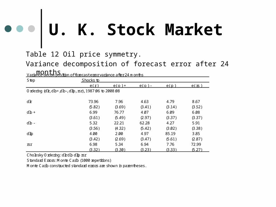
U. K. Stock MarketTable 12 Oil price symmetry. Variance decomposition of forecast error after 24 months.Variance decomposition of forecast error variance after 24 monthsStep Shocks to


dlr 73.96 7.96 4.63 4.79 8.67(5.82) (3.69) (3.41) (3.14) (3.52)

dlo + 6.99 76.77 4.07 6.09 6.08(3.61) (5.49) (2.97) (3.37) (3.37)

dlo - 5.32 22.21 62.28 4.27 5.91(3.56) (4.32) (5.42) (3.02) (3.38)

dlip 4.00 2.00 4.97 85.19 3.85(3.42) (2.69) (3.47) (5.61) (2.87)

rsr 6.98 5.34 6.94 7.76 72.99(3.32) (3.30) (3.23) (3.33) (5.27)


U. K. Stock MarketTable 13 Oil price symmetry .Variance decomposition of forecast error after 24 months.Variance decomposition of forecast error variance after 24 monthsStep Shocks to


dlr 48.90 14.52 19.37 12.27 4.94(11.32) (8.24) (8.28) (8.73) (6.98)

dlo + 26.71 33.28 14.23 15.19 10.59(10.94) (9.64) (8.41) (9.06) (7.31)

dlo - 20.82 26.09 28.39 16.51 8.19(10.13) (8.97) (8.97) (8.64) (6.75)

dlip 11.53 10.05 14.44 57.26 6.72(9.73) (8.64) (8.16) (10.35) (7.37)

rsr 13.21 15.71 12.74 13.34 45.01(9.96) (8.60) (8.37) (8.73) (8.33)


dlr 70.89 7.24 4.25 9.28 8.34(9.80) (7.57) (6.35) (8.28) (6.04)

dlo + 7.89 76.93 6.76 4.81 3.61(5.86) (9.13) (6.60) (6.29) (4.74)

dlo - 9.57 27.60 40.90 8.83 13.11(5.88) (7.89) (7.61) (5.98) (5.87)

dlip 9.15 3.32 9.41 73.24 4.88(6.16) (6.25) (6.95) (8.78) (4.79)

rsr 8.70 10.67 12.36 14.65 53.61(6.10) (7.32) (5.95) (6.54) (7.72)


U. K. Stock MarketTable 14Wald test of symmetry.

Wald Test:Test Statistic Value df Probability

F-statistic 2.158714 (1, 241) 0.143100Chi-square 2.158714 1.000000 0.141800

Null Hypothesis Summary:

Normalized Restriction (= 0) Value Std. Err.

C(4) + C(5) - C(6) - C(7) 0.212001 0.144291

Restrictions are linear in coefficients.


U. K. Stock Market Graph 6; Impulse Response Function for 24 months

-.02

.00

.02

.04

.06

5 10 15 20


-.02

.00

.02

.04

.06

5 10 15 20

Response of DLR to DLO_POS

-.02

.00

.02

.04

.06

5 10 15 20

Response of DLR to DLO_NEG

-.02

.00

.02

.04

.06

5 10 15 20


-.02

.00

.02

.04

.06

5 10 15 20


-.02

.00

.02

.04

.06

5 10 15 20

Response of DLO_POS to DLR

-.02

.00

.02

.04

.06

5 10 15 20

Response of DLO_POS to DLO_POS

-.02

.00

.02

.04

.06

5 10 15 20

Response of DLO_POS to DLO_NEG

-.02

.00

.02

.04

.06

5 10 15 20

Response of DLO_POS to DLIP

-.02

.00

.02

.04

.06

5 10 15 20

Response of DLO_POS to RSR

-.02

.00

.02

.04

.06

5 10 15 20

Response of DLO_NEG to DLR

-.02

.00

.02

.04

.06

5 10 15 20

Response of DLO_NEG to DLO_POS

-.02

.00

.02

.04

.06

5 10 15 20

Response of DLO_NEG to DLO_NEG

-.02

.00

.02

.04

.06

5 10 15 20

Response of DLO_NEG to DLIP

-.02

.00

.02

.04

.06

5 10 15 20

Response of DLO_NEG to RSR

-.008

-.004

.000

.004

.008

.012

5 10 15 20


-.008

-.004

.000

.004

.008

.012

5 10 15 20

Response of DLIP to DLO_POS

-.008

-.004

.000

.004

.008

.012

5 10 15 20

Response of DLIP to DLO_NEG

-.008

-.004

.000

.004

.008

.012

5 10 15 20


-.008

-.004

.000

.004

.008

.012

5 10 15 20


-.02

.00

.02

.04

.06

5 10 15 20


-.02

.00

.02

.04

.06

5 10 15 20

Response of RSR to DLO_POS

-.02

.00

.02

.04

.06

5 10 15 20

Response of RSR to DLO_NEG

-.02

.00

.02

.04

.06

5 10 15 20


-.02

.00

.02

.04

.06

5 10 15 20



Japanese Stock Market The Japanese stock market has experienced a recovery in industrial

production levels following the crisis of 2001, but market still exhibits difficulties in achieving the levels before the bubble burst in 1990.

If the entire study period is considered, the stock market explains 85.33% of its own variance, and the interest rate is the variable that causes the greatest impact on it (5.41%).

If the sub sample is split into two, the interest rate remains the variable that causes the greatest impact on both sub periods.

Japanese Stock Market The interest rate plays an important role in industrial production

during the first sub period (23.02%) and oil prices are variable in the following order of importance. (10.81%), but in the second sub period both variables excrementan its importance in explaining the variance of industrial production.

Japan is more affected by positive petrleros schocks, however the Japanese stock market has demstrado recientmente be more reactive to positive changes in oil prices.

Japanese Stock Market Graph 7; Nikkei225, WTI, Index of IP, interest rate.

0

10,000

20,000

30,000

40,000

90 92 94 96 98 00 02 04 06 08

NIKKEI

0

2

4

6

8

10

90 92 94 96 98 00 02 04 06 08

R

0

20

40

60

80

100

120

140

90 92 94 96 98 00 02 04 06 08

WTI_SPOT

85

90

95

100

105

110

115

90 92 94 96 98 00 02 04 06 08

IIP

Japanese Stock MarketTable 15Unit Root Test; Phillips and Perron (1988)

Phillips and Perron (1988) Unit Root Tests.Variable Adj. t-Stat Probability

In levelslr -1.371931 0.596lo 0.040814 0.9605lip -2.258534 0.1864rsr *** -15.4077 0.0000In first differencesdlr *** -10.0058 0.0000dlo *** -13.78435 0.0000dlip *** -22.07768 0.0000drsr *** -204.1401 0.0001


Japanese Stock MarketTable 16Tests for co-integration using the Johansen procedure

1

1

, `

{ , , }

p

t t t t p t

t

x x x

x lr lo lip

Tests for cointegration using the Johansen procedurePeriod 1988:10 to 2008:08, lag p=12 is chosen using likelihood ratio tests.

Eigenvalues 0.039069 0.017652 0.015961




Japanese Stock MarketTable 17

Variance decomposition of forecast error after 24 months.Variance decomposition of forecast error variance after 24 monthsStep Shocks to


dlr 80.88 6.42 2.52 10.19(6.86) (4.52) (3.31) (5.07)

dlo 6.60 79.57 9.96 3.88(3.63) (5.56) (3.92) (3.52)

dlip 3.88 4.80 82.84 8.48(3.47) (3.73) (6.11) (4.67)

rsr 5.41 4.40 4.86 85.33(3.39) (3.35) (3.80) (5.53)


Japanese Stock MarketTable 18Variance decomposition of forecast error after 24 months.

Variance decomposition of forecast error variance after 24 monthsStep Shocks to


dlr 65.93 8.60 15.26 10.21(11.81) (9.59) (9.32) (10.15)

dlo 12.44 58.42 16.36 12.77(9.91) (11.08) (8.74) (9.42)

dlip 23.02 10.81 57.81 8.36(11.08) (9.84) (11.40) (8.76)

rsr 15.39 14.84 10.57 59.20(10.08) (9.15) (9.40) (11.50)


dlr 68.08 8.62 5.46 17.84(9.23) (7.04) (6.05) (7.63)

dlo 13.94 62.18 11.57 12.30(6.85) (8.51) (6.05) (6.74)

dlip 8.96 5.86 71.64 13.54(7.28) (7.06) (9.95) (8.24)

rsr 12.74 7.33 5.81 74.12(7.26) (6.23) (6.10) (8.76)


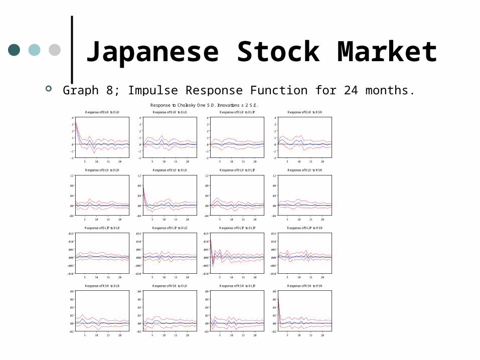
Japanese Stock Market Graph 8; Impulse Response Function for 24 months.

-.2

-.1

.0

.1

.2

.3

.4

5 10 15 20


-.2

-.1

.0

.1

.2

.3

.4

5 10 15 20


-.2

-.1

.0

.1

.2

.3

.4

5 10 15 20


-.2

-.1

.0

.1

.2

.3

.4

5 10 15 20


-.04

.00

.04

.08

.12

5 10 15 20


-.04

.00

.04

.08

.12

5 10 15 20


-.04

.00

.04

.08

.12

5 10 15 20


-.04

.00

.04

.08

.12

5 10 15 20


-.010

-.005

.000

.005

.010

.015

5 10 15 20


-.010

-.005

.000

.005

.010

.015

5 10 15 20


-.010

-.005

.000

.005

.010

.015

5 10 15 20


-.010

-.005

.000

.005

.010

.015

5 10 15 20


-.02

.00

.02

.04

.06

.08

5 10 15 20


-.02

.00

.02

.04

.06

.08

5 10 15 20


-.02

.00

.02

.04

.06

.08

5 10 15 20


-.02

.00

.02

.04

.06

.08

5 10 15 20



Japanese Stock MarketTable 19 Oil price symmetry.

Variance decomposition of forecast error after 24 months.Variance decomposition of forecast error variance after 24 monthsStep Shocks to


dlr 74.76 8.44 4.77 2.22 9.80(6.63) (4.25) (3.63) (2.91) (4.73)

dlo + 3.43 75.09 7.73 7.91 5.85(3.32) (6.20) (3.91) (3.59) (3.80)

dlo - 7.69 22.27 56.10 7.66 6.28(3.94) (4.74) (5.46) (3.53) (3.38)

dlip 3.68 5.94 2.57 79.71 8.11(3.35) (4.06) (3.74) (6.48) (4.42)

rsr 5.33 5.27 3.13 4.98 81.30(3.50) (3.64) (3.20) (3.49) (5.98)


Normalized Restriction (= 0)

Japanese Stock MarketTable 20 Oil price symmetry .Variance decomposition of forecast error after 24 months.Variance decomposition of forecast error variance after 24 monthsStep Shocks to

e( r ) e( o ) + e( o ) - e( p ) e( rs )Ordering (dlr, dlo+,dlo-, dlip, rsr), 1986:01 to 1996:12dlr 58.22 3.86 18.07 14.22 5.64

(13.39) (9.85) (10.19) (9.65) (11.31)dlo + 11.01 36.72 11.10 14.65 26.52

(11.04) (10.56) (9.82) (10.09) (10.99)dlo - 15.59 23.41 30.69 12.81 17.50

(11.66) (10.27) (11.73) (9.71) (10.97)dlip 20.73 11.67 13.43 35.73 18.43

(11.85) (9.96) (10.53) (9.65) (10.97)rsr 18.29 18.82 10.52 10.71 41.66

(11.91) (9.58) (10.32) (9.95) (12.22)


dlr 52.96 16.42 11.11 6.82 12.69(8.90) (6.13) (7.77) (5.91) (7.52)

dlo + 8.39 56.75 9.62 10.17 15.07(6.76) (8.04) (6.38) (6.30) (7.34)

dlo - 16.48 17.03 45.11 11.39 10.00(6.85) (6.17) (7.67) (6.26) (6.70)

dlip 8.41 8.33 5.50 64.77 13.00(7.71) (7.53) (6.92) (9.93) (8.11)

rsr 11.72 5.48 11.65 6.01 65.14(7.23) (5.98) (6.83) (6.30) (8.91)


Japanese Stock MarketTable 21Wald test of symmetry.

Wald Test:

Test Statistic Value df Probability

F-statistic 0.592672 (1, 218) 0.442200Chi-square 0.592672 1.000000 0.441400Null Hypothesis Summary:

Normalized Restriction (= 0)Value Std. Err.

C(4) + C(5) - C(6) - C(7) 0.168590 0.218990

Restrictions are linear in coefficients.


Japanese Stock Market Graph 9; Impulse Response Function for 24 months.

-.2

-.1

.0

.1

.2

.3

.4

5 10 15 20


-.2

-.1

.0

.1

.2

.3

.4

5 10 15 20

Response of DLR to DLO_POS

-.2

-.1

.0

.1

.2

.3

.4

5 10 15 20

Response of DLR to DLO_NEG

-.2

-.1

.0

.1

.2

.3

.4

5 10 15 20


-.2

-.1

.0

.1

.2

.3

.4

5 10 15 20


-.02

.00

.02

.04

.06

5 10 15 20

Response of DLO_POS to DLR

-.02

.00

.02

.04

.06

5 10 15 20

Response of DLO_POS to DLO_POS

-.02

.00

.02

.04

.06

5 10 15 20

Response of DLO_POS to DLO_NEG

-.02

.00

.02

.04

.06

5 10 15 20

Response of DLO_POS to DLIP

-.02

.00

.02

.04

.06

5 10 15 20

Response of DLO_POS to RSR

-.02

.00

.02

.04

.06

5 10 15 20

Response of DLO_NEG to DLR

-.02

.00

.02

.04

.06

5 10 15 20

Response of DLO_NEG to DLO_POS

-.02

.00

.02

.04

.06

5 10 15 20

Response of DLO_NEG to DLO_NEG

-.02

.00

.02

.04

.06

5 10 15 20

Response of DLO_NEG to DLIP

-.02

.00

.02

.04

.06

5 10 15 20

Response of DLO_NEG to RSR

-.010

-.005

.000

.005

.010

.015

5 10 15 20


-.010

-.005

.000

.005

.010

.015

5 10 15 20

Response of DLIP to DLO_POS

-.010

-.005

.000

.005

.010

.015

5 10 15 20

Response of DLIP to DLO_NEG

-.010

-.005

.000

.005

.010

.015

5 10 15 20


-.010

-.005

.000

.005

.010

.015

5 10 15 20


-.02

.00

.02

.04

.06

.08

5 10 15 20


-.02

.00

.02

.04

.06

.08

5 10 15 20

Response of RSR to DLO_POS

-.02

.00

.02

.04

.06

.08

5 10 15 20

Response of RSR to DLO_NEG

-.02

.00

.02

.04

.06

.08

5 10 15 20


-.02

.00

.02

.04

.06

.08

5 10 15 20



Conclusions

The variance of the stock market is affected by changes in oil prices in the U.S. at 9.51%, 7.51% in the United Kingdom UK, and 4.4% in Japan.

The stock market and U.S. industrial production has increased despite higher oil prices. .

Meanwhile, the stock market in the UK is growing but actually industrial sector has shrunk compared to its 2000 level.

Conclusions

Japan has experienced an industrial recovery after the 2001 crisis but its stock market is still showing difficulties to reach the same level as before the economic bubble burst.

The industrial sector of the U.S. is more affected by positive oil shocks (5.22%) than from negative oil shocks (3.36%), while the effect of positive oil shocks (3.88%) into the U.S stock market is less than the effect of negative oil shocks (5.15%).

Conclusions

At the same time, The U.K. economy is always more affected by negative oil shocks, in both its stock market and industrial sector, and Japan is more affected by positive oil shocks, although recently the Japanese stock market had shown to be more reactive to negative oil shocks. 　

　

Conclusions

U.S., interest rate had doubled its importance on causing real stock return changes. It can also be stated from this analysis that interest rate also causes a good proportion of changes in oil prices (23.25%) and industrial production (24.41%).

As a result, it can be stated that interest rate has become more important on the behavior of the real economy, financial sector and energy markets since 1996.

Conclusions

For the U.K., when the Variance decomposition analysis is divided into two periods, it can be seen that interest rate were more important during the first sub period, and also that oil prices and industrial production had increased its importance in the second sub periods.

As a consequence it can be stated that the increment of the stock market in the U.K in the second sub period was produced by rising oil prices rather than a loose monetary policy.

Conclusions

For the economy of Japan if the entire sample period is considered the stock market explains 85.33% of its own variance, and is the interest rate the variable that has more effect on it (5.41%).

If the sample period is split in two, the interest rate remains as the more influential variable on stock markets in the two sub sample periods.

Conclusions

The interest rate plays a major effect on industrial production during the first sub sample period 23.02%, and oil prices is the second more important variable (10.81%), but in the second sub sample period both variables decrease their importance explaining industrial production variance.

This also strengths the idea that Japanese economy, in this case the real economy has become less sensitive to oil prices shocks.

Economy & Finance

Oil schocks