Embed Size (px)
Citation preview

Social media fingerprints of unemployment
Manuel García Herranz (UAM and United Nations, NY)Manuel Cebrián (NICTA, Australia)
Esteban Moro (UC3M, Spain)
Alejandro Llorente (UC3M, Spain)
http://journals.plos.org/plosone/article?id=10.1371/journal.pone.0128692

@llorentealex
Computational Social Science
Data is a reflection of human and groups’ behavior
SocialMobilityActivityContent
SurveysCredit cardMobile phoneSocial mediaSearches…
DemographicsHealthEconomyUnemploymentTransportationGeographyPolitics
Situation Behavior Observation
Individual - Group - City

@llorentealex
Computational Social Science
Economy -> Behavior -> Observation
tie formation. Previous studies have found that in-dividuals benefit from having social ties that bridgebetween communities. These benefits include accessto jobs and promotions (5–13), greater job mobility(14, 15), higher salaries (9, 16, 17), opportunities forentrepreneurship (18, 19), and increased power innegotiations (20, 21). Although these studies sug-gest the possibility that the individual-level bene-fits of having a diverse social networkmay scale tothe population level, the relation between networkstructure and community economic developmenthas never been directly tested (22).
As policy-makers struggle to revive ailing econ-omies, understanding this relation between net-work structure and economic development mayprovide insights into social alternatives to traditionalstimulus policies. To that end,we analyzed themostcomplete record of a national communication net-work studied to date and coupled this social networkdata with detailed socioeconomic indicators to mea-sure this relation directly, at the population level. Thecommunication network data were collected duringthe month of August 2005 in the UK. The datacontain more than 90% of the mobile phones andgreater than 99% of the residential and businesslandlines in the country. The resulting network has65 ! 106 nodes, 368 ! 106 reciprocated social ties, amean geodesic distance (minimumnumber of director indirect edges connecting two nodes) of 9.4, anaverage degree of 10.1 network neighbors, and agiant component (the largest connected subgraph)containing 99.5% of all nodes (23).
Although the nature of this communicationdata limits causal inference, we were able to testthe hypothesized correspondence between socialnetwork structure and economic developmentusing the 2004 UK government’s Index of Mul-tiple Deprivation (IMD), a composite measure ofrelative prosperity of 32,482 communities encom-passing the entire country (24), based on income,employment, education, health, crime, housing,and the environmental quality of each region (25).Each residential landline number was associatedwith the IMD rank of the exchange inwhich it waslocated, as shown in Fig. 1. Obtaining the socio-economic profile for a given telephone exchangearea involves aggregating over the census regionswithin the exchange area. First we uniquelymapped each census region to the exchange areawith which it has the greatest spatial overlap. Wesubsequently aggregated, for each exchange area,the population-weighted average of the IMD forthe census regions assigned to each exchange:
mweighted ! !n
i!1wixi "1#
and
s2weighted ! !n
i!1wi"xi " mweighted#
2 "2#
where xi is the census rank for the ith censusregion that makes up the exchange area and wi isthe population weight of the ith census regiongiven by the fraction of the total population of theexchange area residing in the ith census region.
We then compared the IMD rank of each com-munity with diversity metrics associated with eachmember’s social network. Mobile numbers wereincluded (alongwith landlines) in the calculation ofthe nonspatial diversity measures; however, theywere not used to identifymembers of a community(because of insufficient data on spatial location).Wedeveloped two newmetrics to capture the social andspatial diversity of communication ties within anindividual’s social network. We quantify topolog-ical diversity as a function of the Shannon entropy,
H"i# ! "!k
j!1pij log"pij# "3#
where k is the number of i’s contacts and pij is theproportion of i’s total call volume that involves j, or
pij !Vij
!k
j!1Vij
"4#
where Vij is the volume between node i and j.Wethen define social diversity,Dsocial(i), as the Shannon
entropy associated with individual i’s communi-cation behavior, normalized by k:
Dsocial"i# !"!
k
j!1pij log"pij#
log"k#"5#
The above measure of topological diversitydoes not take into account the geographic diver-sity in the calling patterns within a community.We define a similar measure for spatial diversity,Dspatial(i), by replacing call volume with the geo-graphic distance spanned by an individual’s ties tothe 1992 telephone exchange areas in the UK,
Dspatial"i# !" !
A
a!1pia log"pia#
log"A#"6#
in which pia is the proportion of time i spendscommunicatingwith ath ofA total exchange areas.High diversity scores imply that an individualsplits her time more evenly among social ties andbetween different regions.
Fig. 1. An image of regional communication diversity and socioeconomic ranking for the UK. We findthat communities with diverse communication patterns tend to rank higher (represented from light blueto dark blue) than the regions with more insular communication. This result implies that communicationdiversity is a key indicator of an economically healthy community. [(29) Crown copyright material isreproduced with the permission of the Controller of Her Majesty’s Stationery Office]
21 MAY 2010 VOL 328 SCIENCE www.sciencemag.org1030
REPORTS
on
May
24,
201
0 w
ww
.sci
ence
mag
.org
Dow
nloa
ded
from
Development -> Social/Mobility (city) diversity -> Mobile phonesEagle et al, Science 2010
Soto, V. et al., Prediction of Socioeconomic Levels using Cell Phone Records 2011.
Socio economical level -> Social/Mobility/Activity -> Mobile phones
Antenucci, D. et al., 2014. Using Social Media to Measure Labor Market Flows.
Unemployment -> Content -> Social Media

@llorentealex
Our objective
• It’s not another economical problem in Spain. It is the BIG problem
Unemployment -> Behavior -> Social media (Twitter)
7.9% May 2007
26.3% March 2013

@llorentealex
Geographical areas in Spain
• Municipalities:• ~8200 municipalities in Spain• Very heterogeneous:
population ranging from 7 to 3.2
• We propose a functional approach to the definition of the areas based on daily mobility
• Users’ municipality home is where they tweet most

@llorentealex
Geographical areas in Spain
• We take all trips between two municipalities to construct the flow Tij the number of trips between municipalities
• Flow is well described by the gravity model
ii
“llorenteetal5” — 2014/9/12 — 14:42 — page 2 — #2 ii
ii
ii
Fig. 1. Map of the mobility fluxes Tij between municipalities based on Twitter inferred trips (white). Finally, Infomap communities detected on the network Tij arecolored under the mobility fluxes (blue colors).
Social media dataset and functional partition of citiesTwitter is a microblogging online application where users can expresstheir opinions, share content and receive information from other usersin pieces of 140 characters long, commonly known as tweets. Twitterprovides also social features since a user can follow and be followedby another and also they can interact by mentioning or retweeting(share someone’s tweet with your followers). Some of these tweetscontain information about the location where the user was when thetweet was published, and thus they are geo-located.
To carry out our analysis, we consider 19.6 million geo-locatedTwitter messages (tweet(s)), collected through public API providedby Twitter for the continental part of Spain and from 29th Novem-ber 2012 to 30th June 2013. Tweets were posted by (properlyanonymized) 0.57 Million unique users and geo-positioned in 7683different municipalities. We observed a large correlation (Pearson’scoefficient ⇢ = 0.951[0.949, 0.953]) between the number of geopo-sitioned tweets per municipality and population. On average we findaround 50 tweets per month and per 1000 persons in each municipal-ity.
Despite this high level of social media activity within municipal-ities, we find them not suitable to study socio-economical activity:most of the administrative boundaries between municipalities reflectpolitical and historical decisions, while economical activity happensacross those boundaries. The result is that municipalities in Spainare artificially diverse, ranging from municipalities with only 7 in-habitants to others with 3.2 million population. Although there existsnatural aggregations of municipalities in provinces (regions) or sta-tistical/metropolitan areas, we have used our own data to detect eco-nomical areas. In particular, we have used user daily trips betweenmunicipalities in our database to detect those which are economi-cally related. We say that there is a daily trip between municipality iand j if a user has tweeted in place i and j consecutively within thesame day. In our database we find 1.9 million trips by 0.22 millionusers. With those trips we construct the daily mobility flux networkTij between municipalities as the number of trips between place iand j. Remarkably, the statistical properties of trips and of the mobil-ity matrix Tij coincide with those of other mobility data (see Supp.Matt): for example, trip distance and elapsed time are power law dis-tributed with exponents very similar to those found in the literature.And the mobility fluxes Tij are well described by the Gravity Law(R2
= 0.69)
Tij ' T gravij =
P↵ii P
↵jj
d�ij
where Pi and Pj are the populations of municipalities i and j and dijis the distance between them. These results suggest that, as found inother works, detected mobility from Twitter geo-located tweets is agood proxy of human mobility within and between municipalities.
We use the network of daily fluxes between municipalities Tij todetect the geographical communities of activity. To this end we usestandard partition techniques of the mobility network Tij using graphcommunity finding algorithms. Specifically we have used the In-fomap algorithm and found 340 different communities within Spain.For further details about the comparison among different state-of-artcommunity detection algorithms executed on the inter-city graph, seeSI section III. The average number of municipalities per communityis 21 and the largest community contains 142 municipalities. Thecommunities detected have very interesting features: i) they are cohe-sive geographically, ii) they are statistically robust against randomlyremoval of trips in our database (SI section III, table II), iii) the mod-ularity of the partition is very high. Finally, the partition found hassome overlap with coarser administrative boundaries like provinces(regions). But interestingly, it shows a larger overlap with comarcas
(counties), areas in Spain that reflect geographical and economicalrelations between municipalities. This result shows confirms that themobility detected from geo-located tweets and the communities ob-tained are a good description of economical areas. In the rest of thepaper, we restrict our analysis to the geographical areas defined bythe Infomap detected communities (see figure 1). We discard com-munities which are not formed by at least 5 municipalities, . Despitethis, 99% of the total country of the population is considered in ouranalysis. Similar (although statistically worse) results are obtainedfor municipalites or provinces.
Social media fingerprintsThe goal of this work is to quantify how the behavioral features canbe extracted from social media and then related back to the to theeconomical level of cities. To this end, we define four measures thathave been widely explored in other fields like economy or social sci-ences. All these four measures rely on the identification of the placewhere users live. Instead of using information in the user profile, weanalyze the places where the user has tweeted and we set as home-
town of the user, the municipality where he/she has tweeted with thehighest frequency, a method usually employed in mobile phone andsocial media. To this end we select those users with more than 4 geo-located tweets in our period and which have tweet at least 30% of
2 www.pnas.org/cgi/doi/10.1073/pnas.0709640104 Footline Author
ii
“llorenteetal5” — 2014/9/12 — 14:42 — page 2 — #2 ii
ii
ii
Fig. 1. Map of the mobility fluxes Tij between municipalities based on Twitter inferred trips (white). Finally, Infomap communities detected on the network Tij arecolored under the mobility fluxes (blue colors).
Social media dataset and functional partition of citiesTwitter is a microblogging online application where users can expresstheir opinions, share content and receive information from other usersin pieces of 140 characters long, commonly known as tweets. Twitterprovides also social features since a user can follow and be followedby another and also they can interact by mentioning or retweeting(share someone’s tweet with your followers). Some of these tweetscontain information about the location where the user was when thetweet was published, and thus they are geo-located.
To carry out our analysis, we consider 19.6 million geo-locatedTwitter messages (tweet(s)), collected through public API providedby Twitter for the continental part of Spain and from 29th Novem-ber 2012 to 30th June 2013. Tweets were posted by (properlyanonymized) 0.57 Million unique users and geo-positioned in 7683different municipalities. We observed a large correlation (Pearson’scoefficient ⇢ = 0.951[0.949, 0.953]) between the number of geopo-sitioned tweets per municipality and population. On average we findaround 50 tweets per month and per 1000 persons in each municipal-ity.
Despite this high level of social media activity within municipal-ities, we find them not suitable to study socio-economical activity:most of the administrative boundaries between municipalities reflectpolitical and historical decisions, while economical activity happensacross those boundaries. The result is that municipalities in Spainare artificially diverse, ranging from municipalities with only 7 in-habitants to others with 3.2 million population. Although there existsnatural aggregations of municipalities in provinces (regions) or sta-tistical/metropolitan areas, we have used our own data to detect eco-nomical areas. In particular, we have used user daily trips betweenmunicipalities in our database to detect those which are economi-cally related. We say that there is a daily trip between municipality iand j if a user has tweeted in place i and j consecutively within thesame day. In our database we find 1.9 million trips by 0.22 millionusers. With those trips we construct the daily mobility flux networkTij between municipalities as the number of trips between place iand j. Remarkably, the statistical properties of trips and of the mobil-ity matrix Tij coincide with those of other mobility data (see Supp.Matt): for example, trip distance and elapsed time are power law dis-tributed with exponents very similar to those found in the literature.And the mobility fluxes Tij are well described by the Gravity Law(R2
= 0.69)
Tij ' T gravij =
P↵ii P
↵jj
d�ij
where Pi and Pj are the populations of municipalities i and j and dijis the distance between them. These results suggest that, as found inother works, detected mobility from Twitter geo-located tweets is agood proxy of human mobility within and between municipalities.
We use the network of daily fluxes between municipalities Tij todetect the geographical communities of activity. To this end we usestandard partition techniques of the mobility network Tij using graphcommunity finding algorithms. Specifically we have used the In-fomap algorithm and found 340 different communities within Spain.For further details about the comparison among different state-of-artcommunity detection algorithms executed on the inter-city graph, seeSI section III. The average number of municipalities per communityis 21 and the largest community contains 142 municipalities. Thecommunities detected have very interesting features: i) they are cohe-sive geographically, ii) they are statistically robust against randomlyremoval of trips in our database (SI section III, table II), iii) the mod-ularity of the partition is very high. Finally, the partition found hassome overlap with coarser administrative boundaries like provinces(regions). But interestingly, it shows a larger overlap with comarcas
(counties), areas in Spain that reflect geographical and economicalrelations between municipalities. This result shows confirms that themobility detected from geo-located tweets and the communities ob-tained are a good description of economical areas. In the rest of thepaper, we restrict our analysis to the geographical areas defined bythe Infomap detected communities (see figure 1). We discard com-munities which are not formed by at least 5 municipalities, . Despitethis, 99% of the total country of the population is considered in ouranalysis. Similar (although statistically worse) results are obtainedfor municipalites or provinces.
Social media fingerprintsThe goal of this work is to quantify how the behavioral features canbe extracted from social media and then related back to the to theeconomical level of cities. To this end, we define four measures thathave been widely explored in other fields like economy or social sci-ences. All these four measures rely on the identification of the placewhere users live. Instead of using information in the user profile, weanalyze the places where the user has tweeted and we set as home-
town of the user, the municipality where he/she has tweeted with thehighest frequency, a method usually employed in mobile phone andsocial media. To this end we select those users with more than 4 geo-located tweets in our period and which have tweet at least 30% of
2 www.pnas.org/cgi/doi/10.1073/pnas.0709640104 Footline Author
↵i ⇡ ↵j = 0.42,� = 0.89
R2 = 0.69
Lenormand, M. et al., 2014. Cross-checking different sources of mobility information.

@llorentealex
ii
“llorenteetal5” — 2014/9/12 — 14:42 — page 2 — #2 ii
ii
ii
Fig. 1. Map of the mobility fluxes Tij between municipalities based on Twitter inferred trips (white). Finally, Infomap communities detected on the network Tij arecolored under the mobility fluxes (blue colors).
Social media dataset and functional partition of citiesTwitter is a microblogging online application where users can expresstheir opinions, share content and receive information from other usersin pieces of 140 characters long, commonly known as tweets. Twitterprovides also social features since a user can follow and be followedby another and also they can interact by mentioning or retweeting(share someone’s tweet with your followers). Some of these tweetscontain information about the location where the user was when thetweet was published, and thus they are geo-located.
To carry out our analysis, we consider 19.6 million geo-locatedTwitter messages (tweet(s)), collected through public API providedby Twitter for the continental part of Spain and from 29th Novem-ber 2012 to 30th June 2013. Tweets were posted by (properlyanonymized) 0.57 Million unique users and geo-positioned in 7683different municipalities. We observed a large correlation (Pearson’scoefficient ⇢ = 0.951[0.949, 0.953]) between the number of geopo-sitioned tweets per municipality and population. On average we findaround 50 tweets per month and per 1000 persons in each municipal-ity.
Despite this high level of social media activity within municipal-ities, we find them not suitable to study socio-economical activity:most of the administrative boundaries between municipalities reflectpolitical and historical decisions, while economical activity happensacross those boundaries. The result is that municipalities in Spainare artificially diverse, ranging from municipalities with only 7 in-habitants to others with 3.2 million population. Although there existsnatural aggregations of municipalities in provinces (regions) or sta-tistical/metropolitan areas, we have used our own data to detect eco-nomical areas. In particular, we have used user daily trips betweenmunicipalities in our database to detect those which are economi-cally related. We say that there is a daily trip between municipality iand j if a user has tweeted in place i and j consecutively within thesame day. In our database we find 1.9 million trips by 0.22 millionusers. With those trips we construct the daily mobility flux networkTij between municipalities as the number of trips between place iand j. Remarkably, the statistical properties of trips and of the mobil-ity matrix Tij coincide with those of other mobility data (see Supp.Matt): for example, trip distance and elapsed time are power law dis-tributed with exponents very similar to those found in the literature.And the mobility fluxes Tij are well described by the Gravity Law(R2
= 0.69)
Tij ' T gravij =
P↵ii P
↵jj
d�ij
where Pi and Pj are the populations of municipalities i and j and dijis the distance between them. These results suggest that, as found inother works, detected mobility from Twitter geo-located tweets is agood proxy of human mobility within and between municipalities.
We use the network of daily fluxes between municipalities Tij todetect the geographical communities of activity. To this end we usestandard partition techniques of the mobility network Tij using graphcommunity finding algorithms. Specifically we have used the In-fomap algorithm and found 340 different communities within Spain.For further details about the comparison among different state-of-artcommunity detection algorithms executed on the inter-city graph, seeSI section III. The average number of municipalities per communityis 21 and the largest community contains 142 municipalities. Thecommunities detected have very interesting features: i) they are cohe-sive geographically, ii) they are statistically robust against randomlyremoval of trips in our database (SI section III, table II), iii) the mod-ularity of the partition is very high. Finally, the partition found hassome overlap with coarser administrative boundaries like provinces(regions). But interestingly, it shows a larger overlap with comarcas
(counties), areas in Spain that reflect geographical and economicalrelations between municipalities. This result shows confirms that themobility detected from geo-located tweets and the communities ob-tained are a good description of economical areas. In the rest of thepaper, we restrict our analysis to the geographical areas defined bythe Infomap detected communities (see figure 1). We discard com-munities which are not formed by at least 5 municipalities, . Despitethis, 99% of the total country of the population is considered in ouranalysis. Similar (although statistically worse) results are obtainedfor municipalites or provinces.
Social media fingerprintsThe goal of this work is to quantify how the behavioral features canbe extracted from social media and then related back to the to theeconomical level of cities. To this end, we define four measures thathave been widely explored in other fields like economy or social sci-ences. All these four measures rely on the identification of the placewhere users live. Instead of using information in the user profile, weanalyze the places where the user has tweeted and we set as home-
town of the user, the municipality where he/she has tweeted with thehighest frequency, a method usually employed in mobile phone andsocial media. To this end we select those users with more than 4 geo-located tweets in our period and which have tweet at least 30% of
2 www.pnas.org/cgi/doi/10.1073/pnas.0709640104 Footline Author
• We look for communities in the flow graph • Infomap algorithm
• 340 functional areas were detected:
• They are cohesive
• Statistically robust
• Modularity is high
• High overlap with “comarcas”
(Functional) geographical areas in Spain

Content
Social Interaction
Mobility
Penetration
Activity

@llorentealex
Twitter penetration
• Is Twitter penetration related to economical development of areas?• At country scale twitter penetration ~ GDP
• At small scale is the opposite! twitter penetration ~ unemployment
4
country. All tweeting sources felling below the threshold were discarded from further analysis. In total, the refinement procedure preserved 98% of users and 95% of tweets from the initial database. Definition of a country of the user’s residence
An essential first step in our cross-country mobility analysis was an explicit assignment of each user to a country of residence. This made our work different from the most of other Twitter studies, which usually did not attempt to uncover users’ origin and characterized a study area just with the total volume of tweets observed in this area (e.g. Mocanu et al. 2013). While for certain research problems this approach is suitable, from the perspective of a global mobility study the differentiation between residents and visitors is crucial. It enables a clear definition of origin and destination of travels and reveals which nation is traveling where and when. Taking advantage of the history of tweeting records of every user, we defined her country of residence as the country where the user has issued most of the tweets. Once the country of residence was identified, the user’s activity in any other region of the world was considered as traveling behavior, and the user was counted as a visitor of that country.
We use the country definitions of the Global Administrative Areas spatial database (Global Administrative Areas 2012), which divides the world into 253 territories. Twitter “residents” were identified in 243 of them, with the number of users greatly varying among different countries. The unquestionable leader is USA with over 3.8M users, followed by United Kingdom, Indonesia, Brazil, Japan and Spain with over 500K users each. There are also countries and territories with only few or none Twitter users assigned.
To evaluate the representativeness of Twitter in a given area, a more illustrative metric is the penetration rate, defined as the ratio between the number of Twitter users and the populations of a country. As expected, this ratio does not distribute uniformly across the globe and scales superlinearily with the level of a country economic development approximated by a GDP per capita (Figure 2A and B). While this property has been already described e.g. by Mocanu et al. (2013) the goodness of a fit of a power law approximation increased when considering penetration of just residents rather than all Twitter users appearing in a country. In the analysis we exclude all countries with a penetration rate below 0.05‰ (we also exclude countries with the number of resident users smaller than 10,000).
Figure 2. Twitter penetration rate across countries of the world. (A) Spatial distribution of the index. (B) Superlinear scaling of the penetration rate with per capita GDP of a country. R2 coefficient equals 0.65.
Hawelka, B. et al., 2013. Geo-located Twitter as the proxy for global mobility patterns.
5
10
10 20parofa
ctor
[i] *
tt[, v
aria
bles
_sel
[i]]
% unemp.
Pene
tratio
n ra
te in
dex
⇢ = 0.70 [0.6, 0.77]

@llorentealex
ii
“llorenteetal5” — 2014/8/27 — 22:19 — page 4 — #4 ii
ii
ii
Tweet Detected Misspellings
Alguien se viene con migo aver la vida de PI??
- “Con migo” instead of “Conmigo” (with me in Spanish). - “aver” instead of “a ver” (aver is not a Spanish word)
La quiero mucho y la hecho de menos - “Hecho de menos” instead of “echo de menos” (“I miss her” in Spanish).
All the 618 expressions such as “Con migo”, “Aver” or “Hecho de menos” have been searched literally within the text of the whole dataset of tweets.
●
●
●●
●●●●
●
●
●
●
●●
● ● ●●
●
●
●●
●
●●
●●●
●
●
●
●
●●
● ●●
●
●
●
A B
Entropy: 0.72Unemployment rate: 11%
Entropy: 0.42Unemployment rate: 23%
A B
C
2.5
5.0
7.5
10.0
5 10 15 20hour
fraction mun
ab%
of t
wee
ts
Proportion of tweets
Hour
Low unemp. rateHigh unemp. rate
Fig. 3. Examples of differnt behavior in the observed variables and the unemployment. In A, we observe that two cities with different unemployment levels have
different temporal activity patterns. Figure B show how cities with distinct entropy levels may hold different unemployment intensity. Finally, figure C shows some
examples of detected misspellings in our database.
●
●
●
●
●
●
●
●
●
●
●
●
●
●
●
●
●
●
●
●
●
●
●
●
●
●
eco
unemp
emp
job
fmiss
madrugada
tarde
manana
siorsocial
siosocial
sior
sio
rtwpen
−0.5 0.0 0.5corre
ff
500
1000
10 20parofa
ctor
[i] *
tt[, v
aria
bles
_sel
[i]]
20
40
60
80
10 20parofa
ctor
[i] *
tt[, v
aria
bles
_sel
[i]]
20
40
60
80
1020paro fa
ctor[i] * tt[, variables_sel[i]]
20
40
60
80
1020paro fa
ctor[i] * tt[, variables_sel[i]]
0
5
10
15
20
10 20parofa
ctor
[i] *
tt[, v
aria
bles
_sel
[i]]
0
5
10
15
20
1020paro fa
ctor[i] * tt[, variables_sel[i]]
0
5
10
15
20
1020paro fa
ctor[i] * tt[, variables_sel[i]]
4
5
6
7
10 20parofa
ctor
[i] *
tt[, v
aria
bles
_sel
[i]]
5
10
10 20parofa
ctor
[i] *
tt[, v
aria
bles
_sel
[i]]
40
50
60
70
10 20parofa
ctor
[i] *
tt[, v
aria
bles
_sel
[i]]
0.2
0.4
0.6
0.8
10 20parofa
ctor
[i] *
tt[, v
aria
bles
_sel
[i]]
0
50
100
150
200
10 20parofa
ctor
[i] *
tt[, v
aria
bles
_sel
[i]]
0
50
100
150
200
10 20parofa
ctor
[i] *
tt[, v
aria
bles
_sel
[i]]
0
50
100
150
200
10 20parofa
ctor
[i] *
tt[, v
aria
bles
_sel
[i]]
Penetration rate Entropy1 (geo) Entropy2 (geo)
Entropy1 (social) Entropy2 (social) Activity (morning)
Activity (afternoon) Activity (night)
Misspellers rate #Job tweets
#Employment tws #Unemployment tws
#Economy tws !!
a) b) c)
d) e)
% Unemployment % UnemploymentCorrelation
Entropy1 (social)
Misspellers rate
Pen
etra
tion
rate
Act
ivity
(mro
ning
)
Fig. 4. Correlation of the measures with the unemployment rate
x
y
6 10 15 20 25
810
1520
30
Observed unemployment % (u) 6 10 15 20 25
Pre
dict
ed u
nem
ploy
men
t % (u
* )
8
10
15
20
30
Linear Model
± 0.2 u
Variable Weight
Penetration Rate 32,18
Geo-social entropy 7,25 *
Morning activity % 20,52
Misspellers % 40,16
R2 = 0.536p-value < 2.2e-16
* not statistically significant
Fig. 5. Performance of the model, showing the predicted unemployment rate versus the observed one, R2 = 0.536. It also shows a table containing the weight
for each considered variable.
from the digital traces that are left by the use of social media. In par- ticular, we show how behavioral features related to unemployment
4 www.pnas.org/cgi/doi/10.1073/pnas.0709640104 Footline Author
Act
ivity
(% tw
eets
)
Entropy: 0.42 Unemployment: 20.3%
Entropy: 0.72 Unemployment: 8.8%
●
●
●
●
●
●
●
●
●
●
●
●
●
●
●
●
●
●
●
●
●
●
A
C
B
Twitter social interactions• Granovetter: diversity of interactions yields to more opportunities
• Diversity of interactions between cities is correlated with economical development
• We construct the graph of social interactions
• Measure diversity with entropy
% unempEn
tropy
(%)
Eagle et al, Science 2010
wij = number of @ between areas i and jpij = wij/
Pki
j=1 wij
Si = �Pki
j=1 pij log pij
20
40
60
80
10 20parofa
ctor
[i] *
tt[, v
aria
bles
_sel
[i]]
⇢ = �0.21[�0.37,�0.04]

@llorentealex
Twitter geographical interactions• Diversity of geographical mobility is correlated with development
• We use the graph of flows
• Measure diversity with entropy
% unemp
Entro
py (%
)
Smith, C., Mashhadi, A. & Capra, L., 2013. Ubiquitous sensing for mapping poverty in developing countries.Smith, C., Quercia, D. & Capra, L., 2013. Finger on the pulse: identifying deprivation using transit flow analysis.Smith, C., Quercia, D. & Capra, L., 2013. Finger on the pulse: identifying deprivation using transit flow analysis. pp.683–692.
˜Si = �Pk̃i
j=1 p̃ij log p̃ij
p̃ij = Tij/Pk̃i
j=1 Tij
0.1
0.2
0.3
0.4
10 20paro
tt[, "
sio"
]
⇢ = �0.023 [�0.19, 0.14]

@llorentealex
Twitter content
• Two different approaches• Classical approach: NLP applied to detect mentions to “unemployment”,
“job”, “economy”, …• Antenucci, D. et al., 2014. Using Social Media to Measure Labor Market Flows.
)LJXUH�����,QLWLDO�&ODLPV�IRU�8QHPSOR\PHQW�,QVXUDQFH�DQG�-RE�/RVV�DQG�8QHPSOR\PHQW�)DFWRU����
�1RWH���)LJXUH�VKRZV�WKH�'HSDUWPHQW�RI�/DERU¶V�,QLWLDO�&ODLPV�IRU�8QHPSOR\PHQW�,QVXUDQFH��OHIW�VFDOH��UHYLVHG�GDWD��VHDVRQDOO\�DGMXVWHG��DQG�WKH�6RFLDO�0HGLD�)DFWRU����ULJKW�VFDOH����7KH�IDFWRU�LV�HVWLPDWHG�DV�GHVFULEHG�LQ�WKH�WH[W�DQG�LV�QR�ZD\�ILW�WR�WKH�LQLWLDO�FODLPV�GDWD��� �
Thou
sand
s Factor 1
2011 2012 2013280
300
320
340
360
380
400
420
440
460
-10
-5
0
5
10
15
20Initial Claims (lef t scale)
Social Media (right scale)
0.000
0.001
0.002
10 20paro
tt[, "
emp"
]
% unemp
#men
tions
to e
mpl
oym
ent
⇢ = �0.33 [�0.17,�0.47]
@llorentealex
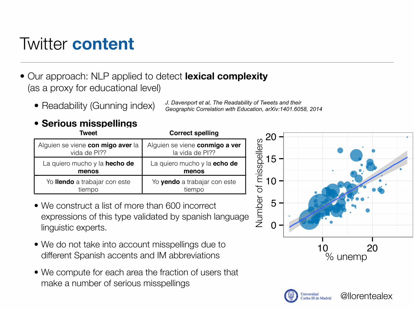
Twitter content• Our approach: NLP applied to detect lexical complexity
(as a proxy for educational level)
• Readability (Gunning index)
• Serious misspellings
•
• We construct a list of more than 600 incorrect expressions of this type validated by spanish language linguistic experts.
• We do not take into account misspellings due to different Spanish accents and IM abbreviations
• We compute for each area the fraction of users that make a number of serious misspellings
Tweet Correct spelling
Alguien se viene con migo aver la vida de PI??
Alguien se viene conmigo a ver la vida de PI??
La quiero mucho y la hecho de menos
La quiero mucho y la echo de menos
Yo llendo a trabajar con este tiempo
Yo yendo a trabajar con este tiempo
J. Davenport et al, The Readability of Tweets and their Geographic Correlation with Education, arXiv:1401.6058, 2014
0
5
10
15
20
10 20parofa
ctor
[i] *
tt[, v
aria
bles
_sel
[i]]
% unempNu
mbe
r of m
isspe
llers

@llorentealex
Twitter activity
• Is unemployment reflected in twitter daily patterns?Just arrived to work, mondays are too hard…
ii
“llorenteetal5” — 2014/8/27 — 22:19 — page 4 — #4 ii
ii
ii
Tweet Detected Misspellings
Alguien se viene con migo aver la vida de PI??
- “Con migo” instead of “Conmigo” (with me in Spanish). - “aver” instead of “a ver” (aver is not a Spanish word)
La quiero mucho y la hecho de menos - “Hecho de menos” instead of “echo de menos” (“I miss her” in Spanish).
All the 618 expressions such as “Con migo”, “Aver” or “Hecho de menos” have been searched literally within the text of the whole dataset of tweets.
●
●
●●
●●●●
●
●
●
●
●●
● ● ●●
●
●
●●
●
●●
●●●
●
●
●
●
●●
● ●●
●
●
●
A B
Entropy: 0.72Unemployment rate: 11%
Entropy: 0.42Unemployment rate: 23%
A B
C
2.5
5.0
7.5
10.0
5 10 15 20hour
fraction mun
ab%
of t
wee
ts
Proportion of tweets
Hour
Low unemp. rateHigh unemp. rate
Fig. 3. Examples of differnt behavior in the observed variables and the unemployment. In A, we observe that two cities with different unemployment levels have
different temporal activity patterns. Figure B show how cities with distinct entropy levels may hold different unemployment intensity. Finally, figure C shows some
examples of detected misspellings in our database.
●
●
●
●
●
●
●
●
●
●
●
●
●
●
●
●
●
●
●
●
●
●
●
●
●
●
eco
unemp
emp
job
fmiss
madrugada
tarde
manana
siorsocial
siosocial
sior
sio
rtwpen
−0.5 0.0 0.5corre
ff
500
1000
10 20parofa
ctor
[i] *
tt[, v
aria
bles
_sel
[i]]
20
40
60
80
10 20parofa
ctor
[i] *
tt[, v
aria
bles
_sel
[i]]
20
40
60
80
1020paro fa
ctor[i] * tt[, variables_sel[i]]
20
40
60
80
1020paro fa
ctor[i] * tt[, variables_sel[i]]
0
5
10
15
20
10 20parofa
ctor
[i] *
tt[, v
aria
bles
_sel
[i]]
0
5
10
15
20
1020paro fa
ctor[i] * tt[, variables_sel[i]]
0
5
10
15
20
1020paro fa
ctor[i] * tt[, variables_sel[i]]
4
5
6
7
10 20parofa
ctor
[i] *
tt[, v
aria
bles
_sel
[i]]
5
10
10 20parofa
ctor
[i] *
tt[, v
aria
bles
_sel
[i]]
40
50
60
70
10 20parofa
ctor
[i] *
tt[, v
aria
bles
_sel
[i]]
0.2
0.4
0.6
0.8
10 20parofa
ctor
[i] *
tt[, v
aria
bles
_sel
[i]]
0
50
100
150
200
10 20parofa
ctor
[i] *
tt[, v
aria
bles
_sel
[i]]
0
50
100
150
200
10 20parofa
ctor
[i] *
tt[, v
aria
bles
_sel
[i]]
0
50
100
150
200
10 20parofa
ctor
[i] *
tt[, v
aria
bles
_sel
[i]]
Penetration rate Entropy1 (geo) Entropy2 (geo)
Entropy1 (social) Entropy2 (social) Activity (morning)
Activity (afternoon) Activity (night)
Misspellers rate #Job tweets
#Employment tws #Unemployment tws
#Economy tws !!
a) b) c)
d) e)
% Unemployment % UnemploymentCorrelation
Entropy1 (social)
Misspellers rate
Pen
etra
tion
rate
Act
ivity
(mro
ning
)
Fig. 4. Correlation of the measures with the unemployment rate
x
y
6 10 15 20 25
810
1520
30
Observed unemployment % (u) 6 10 15 20 25
Pre
dict
ed u
nem
ploy
men
t % (u
* )
8
10
15
20
30
Linear Model
± 0.2 u
Variable Weight
Penetration Rate 32,18
Geo-social entropy 7,25 *
Morning activity % 20,52
Misspellers % 40,16
R2 = 0.536p-value < 2.2e-16
* not statistically significant
Fig. 5. Performance of the model, showing the predicted unemployment rate versus the observed one, R2 = 0.536. It also shows a table containing the weight
for each considered variable.
from the digital traces that are left by the use of social media. In par- ticular, we show how behavioral features related to unemployment
4 www.pnas.org/cgi/doi/10.1073/pnas.0709640104 Footline Author
Act
ivity
(% tw
eets
)
Entropy: 0.42 Unemployment: 20.3%
Entropy: 0.72 Unemployment: 8.8%
●
●
●
●
●
●
●
●
●
●
●
●
●
●
●
●
●
●
●
●
●
●
A
C
B
●
●
●
●
●
●
●
●
●
●
●
●
●
●
●
●
●
●
●
●
●
●
●
●
●
●
eco
unemp
emp
job
fmiss
madrugada
tarde
manana
siorsocial
siosocial
sior
sio
rtwpen
−0.5 0.0 0.5corre
ff
500
1000
10 20parofa
ctor
[i] *
tt[, v
aria
bles
_sel
[i]]
20
40
60
80
10 20parofa
ctor
[i] *
tt[, v
aria
bles
_sel
[i]]
20
40
60
80
1020paro fa
ctor[i] * tt[, variables_sel[i]]
20
40
60
80
1020paro fa
ctor[i] * tt[, variables_sel[i]]
0
5
10
15
20
10 20parofa
ctor
[i] *
tt[, v
aria
bles
_sel
[i]]
0
5
10
15
20
1020paro fa
ctor[i] * tt[, variables_sel[i]]
0
5
10
15
20
1020paro fa
ctor[i] * tt[, variables_sel[i]]
4
5
6
7
10 20parofa
ctor
[i] *
tt[, v
aria
bles
_sel
[i]]
5
10
10 20parofa
ctor
[i] *
tt[, v
aria
bles
_sel
[i]]
40
50
60
70
10 20parofa
ctor
[i] *
tt[, v
aria
bles
_sel
[i]]
0.2
0.4
0.6
0.8
10 20parofa
ctor
[i] *
tt[, v
aria
bles
_sel
[i]]
0
50
100
150
200
10 20parofa
ctor
[i] *
tt[, v
aria
bles
_sel
[i]]
0
50
100
150
200
10 20parofa
ctor
[i] *
tt[, v
aria
bles
_sel
[i]]
0
50
100
150
200
10 20parofa
ctor
[i] *
tt[, v
aria
bles
_sel
[i]]
Penetration rate Entropy1 (geo) Entropy2 (geo)
Entropy1 (social) Entropy2 (social) Activity (morning)
Activity (afternoon) Activity (night)
Misspellers rate #Job tweets
#Employment tws #Unemployment tws
#Economy tws !!
a) b) c)
d) e)
% Unemployment % UnemploymentCorrelation
Entropy1 (social)
Misspellers rate
Pen
etra
tion
rate
Act
ivity
(mro
ning
)
⇢ = �0.48 [�0.34,�0.60]

@llorentealex
Summary of the variables
●
●
●
●
●
●
●
●
●
●
●
●
●
●
●
●
●
●
●
●
●
●
●
●
●
●
eco
unemp
emp
job
fmiss
madrugada
tarde
manana
siorsocial
siosocial
sior
sio
rtwpen
−0.5 0.0 0.5corre
ff
500
1000
10 20parofa
ctor
[i] *
tt[, v
aria
bles
_sel
[i]]
20
40
60
80
10 20parofa
ctor
[i] *
tt[, v
aria
bles
_sel
[i]]
20
40
60
80
1020paro fa
ctor[i] * tt[, variables_sel[i]]
20
40
60
80
1020paro fa
ctor[i] * tt[, variables_sel[i]]
0
5
10
15
20
10 20parofa
ctor
[i] *
tt[, v
aria
bles
_sel
[i]]
0
5
10
15
20
1020paro fa
ctor[i] * tt[, variables_sel[i]]
0
5
10
15
20
1020paro fa
ctor[i] * tt[, variables_sel[i]]
4
5
6
7
10 20parofa
ctor
[i] *
tt[, v
aria
bles
_sel
[i]]
5
10
10 20parofa
ctor
[i] *
tt[, v
aria
bles
_sel
[i]]
40
50
60
70
10 20parofa
ctor
[i] *
tt[, v
aria
bles
_sel
[i]]
0.2
0.4
0.6
0.8
10 20parofa
ctor
[i] *
tt[, v
aria
bles
_sel
[i]]
0
50
100
150
200
10 20parofa
ctor
[i] *
tt[, v
aria
bles
_sel
[i]]
0
50
100
150
200
10 20parofa
ctor
[i] *
tt[, v
aria
bles
_sel
[i]]
0
50
100
150
200
10 20parofa
ctor
[i] *
tt[, v
aria
bles
_sel
[i]]
Penetration rate Entropy1 (geo) Entropy2 (geo)
Entropy1 (social) Entropy2 (social) Activity (morning)
Activity (afternoon) Activity (night)
Misspellers rate #Job tweets
#Employment tws #Unemployment tws
#Economy tws !!
a) b) c)
d) e)
% Unemployment % UnemploymentCorrelation
Entropy1 (social)
Misspellers rate
Pen
etra
tion
rate
Act
ivity
(mro
ning
)
Social/geo variables have low correlationPenetration rate/activity and content are highly correlated with unemployment

@llorentealex
Explanatory power of Twitter variables
x
y
5 10 15 20 25
510
1520
25
% Unemployment (real)
% U
nem
ploy
men
t (pr
edict
ed)
• Simple linear regression
Penetration
Entropy (social)
Activity (morning)
#misspellers
"unemployment"
0 10 20 30 40
*
% weight in the model
R2 = 0.64
@llorentealex
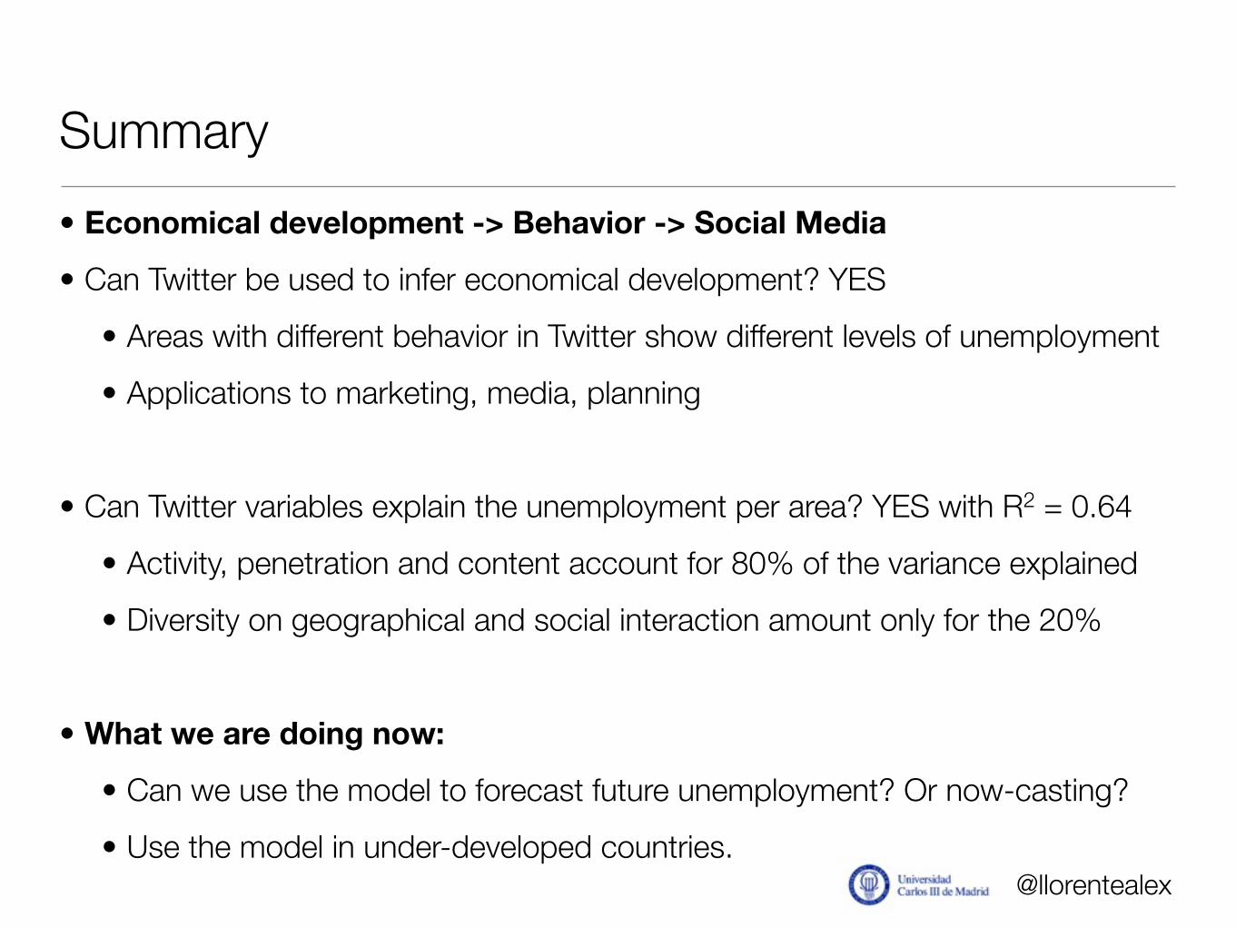
Summary• Economical development -> Behavior -> Social Media
• Can Twitter be used to infer economical development? YES• Areas with different behavior in Twitter show different levels of unemployment• Applications to marketing, media, planning
• Can Twitter variables explain the unemployment per area? YES with R2 = 0.64• Activity, penetration and content account for 80% of the variance explained• Diversity on geographical and social interaction amount only for the 20%
• What we are doing now:
• Can we use the model to forecast future unemployment? Or now-casting?• Use the model in under-developed countries.