Embed Size (px)
Citation preview

Understanding the Transition Pattern of Synchronization Stability in Power Grids
May 30– June 3, 2016 Seoul, South Korea
Heetae Kim , Petter Holme Department of Energy Science, Sungkyunkwan University, South Korea
Sang Hoon Lee Korea Institute for Advanced Study, South Korea
AMERICA REVEALED - Power black-outs, PBS

http://www.nydailynews.com/news/national/northeast-blackout-2003-ten-year-anniversary-article-1.1426561


Understanding the Transition Pattern of Synchronization Stability in Power Grids
May 30– June 3, 2016 Seoul, South Korea
1 Department of Energy Science, Sungkyunkwan University, South Korea
2 Korea Institute for Advanced Study, South Korea
Sang Hoon Lee 2 Petter Holme 1Heetae Kim 1

May 30– June 3, 2016 Seoul, South Korea
• Power-grid generation models
• Static network ‣ Vulnerability against local failure or terrorist attack.
‣ The structural analyses of real power grids(North America, Italy, and so on)
• Dynamic network ‣ The dynamic phenomena such as cascading propagation.
‣ Synchronization stability
Understanding the Transition Pattern of Synchronization Stability in Power Grids

Synchronization in power grids
https://youtu.be/RT1ySBc-Blshttps://youtu.be/tiKH48EMgKE
Phase locked (synchronized)
i j
Power plant (P>0)
Power plant (P>0)
Consumer (P<0)
✓Phase of alternating current (AC) of motors at load or rotors in power generators

Synchronization in power grids
i j
Power plant (P>0)
Power plant (P>0)
Consumer (P<0)
Not in synchrony
Synchronized (Phase-locked)
✓Phase of alternating current (AC) of motors at load or rotors in power generators
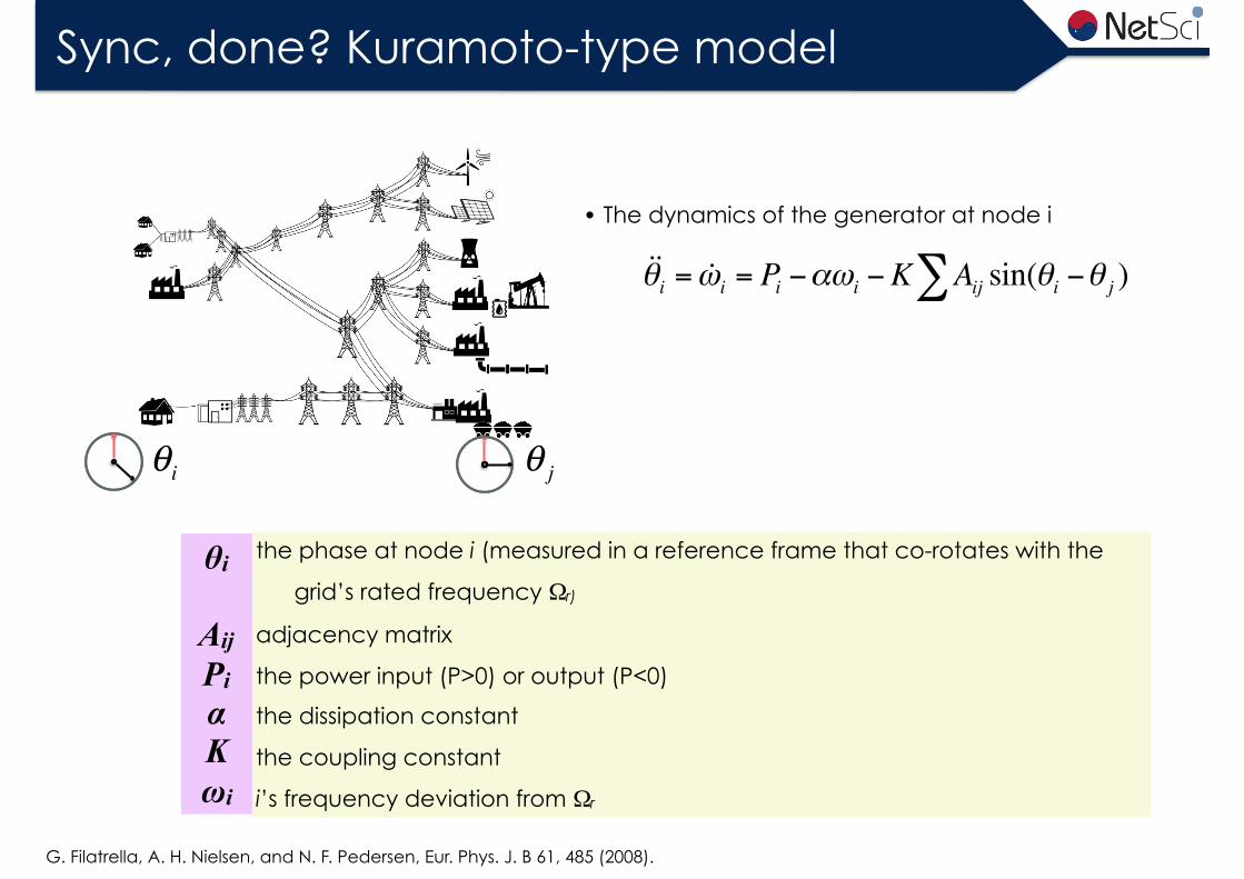
Sync, done? Kuramoto-type model
!!θi = !ωi = Pi −αωi −K Aij sin(θi −θ j )∑
the phase at node i (measured in a reference frame that co-rotates with the
grid’s rated frequency Ωr)
adjacency matrix
the power input (P>0) or output (P<0)
the dissipation constant
the coupling constant
i’s frequency deviation from Ωr
θi
Aij Pi α K ωi
G. Filatrella, A. H. Nielsen, and N. F. Pedersen, Eur. Phys. J. B 61, 485 (2008).
• The dynamics of the generator at node i
θi θ j

Sync, done? Kuramoto-type model
the phase angle of voltage at node i (measured in a reference frame that co-
rotates with the grid’s rated frequency Ωr)
adjacency matrix
the power input (P>0) or output (P<0)
the dissipation constant
the coupling constant
i’s frequency deviation from Ωr
θi
Aij Pi α K ωi
θi θ j
G. Filatrella, A. H. Nielsen, and N. F. Pedersen, Eur. Phys. J. B 61, 485 (2008).
K
!!θi = !ωi = Pi −αωi −K Aij sin(θi −θ j )∑• The dynamics of the generator at node i

Sync, stable? Basin stability
Basin stability∈[0,1] =
✓How much a node can recover synchrony
P. J. Menck, J. Heitzig, N. Marwan, and J. Kurths, Nat Phys 9, 89 (2013).https://youtu.be/dFjf_d69HtY
Synchronization
Desynchronization

Basin stability: application example
P. J. Menck, J. Heitzig, J. Kurths, and H. Joachim Schellnhuber, Nat Comms 5, 3969 (2014).
<Northern European power grid>

Sync stability, change!
Otherwise, it will converge to a different solution of (1)! (2): anon-synchronous limit cycle characterized by
onsðtÞ $Paþ aK
Pcos
Pa
t! "
ð3Þ
(provided |P|/a2c1, |P|2/a2cK, see Supplementary Note 1).Other, possibly serial, faults may push the generator from the
synchronous state to perturbed states anywhere in state space. If,for instance, the turning on of a major load or a large fluctuationin renewable generation temporarily drove P below zero, thegenerator’s state would deviate into the lower half of state space(see illustrative trajectory 2 in Fig. 1a). Clearly, the synchronousbasin should be as large as possible. We therefore quantify howstable the synchronous state is against general large perturbationsin terms of basin stability S, a measure of the basin’s volume20.
Specifically, we define basin stability as
SðBÞ ¼Z
wBðy;oÞ rðy;oÞ dy do: ð4Þ
Here
wBðy;oÞ ¼1 ifðy;oÞ 2 B0 otherwise
#ð5Þ
is the indicator function of the synchronous state’s basin B and r isa density with
Rr(y, o) dydo¼ 1 that reflects to which states in
state space the system may be pushed by large perturbations. Thenumber SA[0,1] expresses the likelihood that the system returns tothe synchronous state after having been hit by a large perturbationoccuring randomly according to the probability density r. S¼ 0when synchrony is unstable, and S¼ 1 when it is globally stable.We estimate basin stability by means of a numerical Monte-Carloprocedure20–22: draw T random initial states according to r,simulate the associated trajectories, and count the number U oftimes the system converges to the synchronous state. Then SEU/T. We use T¼ 500 throughout this paper, which yields20 astandard error of e ¼
ffiffiffiffiffiffiffiffiffiffiffiffiffiffiffiffiS 1! Sð Þ
p=ffiffiffiffiTp
o0:023.Intuition suggests that the synchronous state should become
more stable when the transmission line’s transfer capacity Kincreases. This is indeed what we find: the expanding green areain Fig. 1a–c and the characteristic in Fig. 1d show that basinstability S, starting from S¼ 0 for Ko|P|, improves substantiallyas K goes up, until finally synchrony becomes the only stable state(S¼ 1). Here we have chosen a uniform distribution restricted to
a large box in state space, namely
rðy;oÞ ¼ 1= jQj ifðy;oÞ 2 Q0 otherwise
#;whereQ ¼ ½0; 2p()½! 100; 100(:
ð6ÞThis choice allows to clearly distinguish the three important casesin which B covers (i) significantly less than half of statespace (Fig. 1a); (ii) about half of state space (Fig. 1b); and(iii) all of state space (Fig. 1c). We keep using this choice of r inthe following.
Multinode model. The one-node model of equations (1 and 2) isof course a strong simplification: there will be some interplaybetween multiple nodes after one of them has been hit by a largeperturbation, and whether or not the grid will return to syn-chrony depends on the affected node’s properties, particularly itsposition within the grid topology. Hence, we now turn to anN-node version of the model that captures in a coarse-grainedway12,13,17 the decisive electromechanical interactions takingplace in the transmission grid after a large perturbation (seeMethods). It reads
_yi ¼ oi ð7Þ
_oi ¼ ! aioiþPi!XN
j¼1
Kij sin ðyi! yjÞ ð8Þ
where yi and oi denote phase and frequency of the generator atnode i, and ai and Pi are its damping constant and net powerinput. We refer to nodes with Pi40 as net generators and tonodes with Pio0 as net consumers. The matrix {Kij} reflects thewiring topology, with Kij¼Kji40 if nodes i and j are connected,and Kij¼ 0 otherwise.
Power grids do possess stable non-synchronousstates5,12,13,17,18. We assume that there is also a stablesynchronous state with constant phases ys
i and frequenciesoi¼ 0, and with basin of attraction B. How stable is this stateagainst large local perturbations that affect a single node? Andhow does this depend on the network topology? Before turning toa case study of the Northern European power grid, we addressthese questions statistically by studying an ensemble of 1,000randomly generated power grids with N¼ 100 nodes and E¼ 135transmission lines. These numbers yield the average degree/dS¼ 2.7, a value typical of power transmission grids23. Tofocus on the topology, we simplify generator and transmission
1
0.75
0.25
0.50
0
K
S
0 10 20 30 40 50 60 70
15
0
–15
15
0
–15
0 0
!
!
15
0
–15
!
–" –"" "# – #s
(#, !)t1
(#s, 0) = (#, !)t0
Stable limit cycle
Trajectory 1
Trajectory 2
# – #s
0–" "
Figure 1 | Basin stability of the generator in the one-node model. (a–c) State space of the model (1)! (2), with a¼0.1, P¼ 1 and (a) K¼8,(b) K¼ 24, (c) K¼ 65 (see Methods). The solid black circle marks the desired synchronous state (ys,0), and the solid red line shows the undesirednon-synchronous limit cycle attractor. The basin of attraction of (ys, 0) is coloured green, and that of the limit cycle is coloured white. In (a), the greydashed line indicates the fault-on (K¼0) trajectory 1 and its end point (y, o)t1
. The dash-dotted line indicates the fault-on (K¼ 8, P¼ !6) trajectory 2.(d) Basin stability S of the synchronous state versus the transmission capacity K.
NATURE COMMUNICATIONS | DOI: 10.1038/ncomms4969 ARTICLE
NATURE COMMUNICATIONS | 5:3969 | DOI: 10.1038/ncomms4969 | www.nature.com/naturecommunications 3
& 2014 Macmillan Publishers Limited. All rights reserved.
K=8 K=24 K=65
P. J. Menck, J. Heitzig, J. Kurths, and H. Joachim Schellnhuber, Nat Comms 5, 3969 (2014).
✓Synchronization stability changes according to the transmission strength

Sync stability, change, abruptly!
0
50
100
150
0 1
Num
ber o
f nod
es
Basin stabilityat K=1.2710
0 1Basin stabilityat K=1.2715
0 1Basin stabilityat K=1.2720
0 1Basin stabilityat K=1.2725
Num
ber o
f nod
es
0
1
Bas
in st
abili
ty
✓It is necessary to understand the entire transition
H. Kim, S. H. Lee, P. Holme, New J. Phys. 17, 113005 (2015).

Various transition shapes
0
1
0 20 40
Producer Consumer
Bas
in s
tabil
ity
K
Node A, DNode B, C
A B C D
✓The basin stability transition form varies in a network.
0
0.5
1
0 10 20
(a) (b)
Bas
in s
tab
ilit
y
K
Node 2Node 5
1 2
3 4 5 6
7 8
0
0.5
1
0 10 20
(a) (b)
Bas
in s
tab
ilit
y
K
Node 2Node 5
1 2
3 4 5 6
7 8
0
1
0 20 40
Producer Consumer
Bas
in s
tabil
ity
K
Node A, DNode B, C
A B C D
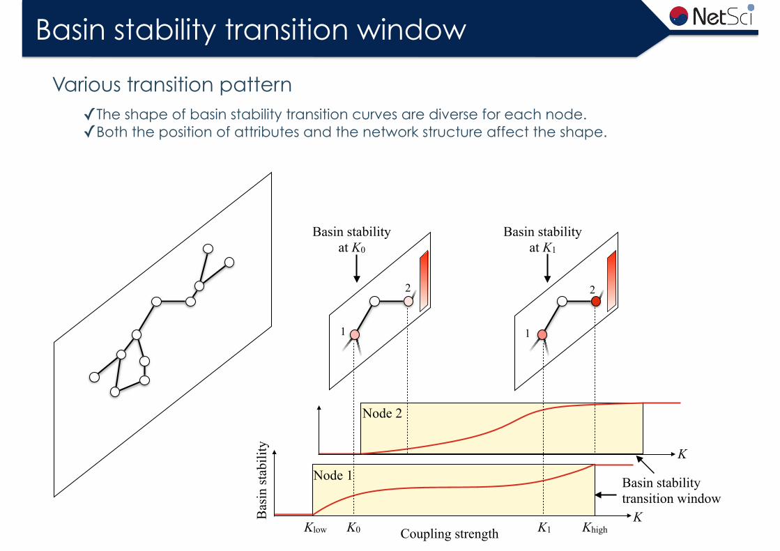
Basin stability transition window
K
K
Bas
in st
abili
ty
Coupling strength
1
2
1
2
Basin stability transition window
Basin stability at K0
K0 K1
Basin stability at K1
Node 1
Node 2
Klow Khigh
✓The shape of basin stability transition curves are diverse for each node. ✓Both the position of attributes and the network structure affect the shape.
Various transition pattern

Network generation
<Transmission system dada>
Node (Poser plant)
Link (Transmission line)
Agua santa
PlacillaNode
(Substation)
CDEC-SIC Annual report (2014)
• 420 nodes ↳129 power plants
291 substations • 543 edges

Transition windows of Chilean power grid
0
0.2
0.4
0.6
0.8
1
0 5 10 15 20
(a)
Bas
in st
abili
ty
K
Node ANode BNode C
0 5 10 15
(a) (b)
10-3−10-2
10-2−10-1
10-1−100
100−101
101−102
<K range>
K 0 1
Proportion
0 20
∆K
Kmid
0
0.2
0.4
0.6
0.8
1
0 5 10 15 20
(a)
Bas
in st
abili
ty
K
Node 80Node 286Node 283
0 5 10 15
(a) (b)
10-3−10-2
10-2−10-1
10-1−100
100−101
101−102
<K range>
K 0 1
Proportion
0 20
∆K
Kmid
0
∆K max
H. Kim, S. H. Lee, P. Holme, New J. Phys. 17, 113005 (2015).
✓Heterogeneous distribution of ∆K range
(a) (b)
(c) (d)6
2
4
A 0
0.2
0.4
0.6
0.8
1
0 2 4 6 8 10 12 14 16
Bas
in st
abili
ty
K
node Anode Bnode Cnode Dnode Enode Fnode G
B
C
D
E
FG
1
5
3 0
0.2
0.4
0.6
0.8
1
0 5 10 15 20 25
Bas
in st
abili
ty
K
node 1node 2node 3node 4node 5node 6
(a) (b)
(c) (d)6
2
4
A 0
0.2
0.4
0.6
0.8
1
0 2 4 6 8 10 12 14 16
Bas
in st
abili
ty
K
node Anode Bnode Cnode Dnode Enode Fnode G
B
C
D
E
FG
1
5
3 0
0.2
0.4
0.6
0.8
1
0 5 10 15 20 25
Bas
in st
abili
ty
K
node 1node 2node 3node 4node 5node 6

Community detection
Mucha P J and Porter M A GenLouvain http://netwiki.amath.unc.edu/GenLouvain/GenLouvain
✓Consistent vs inconsistent community membership Simulations

Community consistency
φi : community consistency of node i.φij : the fraction of the case that node i and j are assigned to the same community for series of community detections.N : the number of nodes.
�i =1
N�1
Pj 6=i(1� 2�ij)2
1
3
2 1
3
21
3
2 1
3
2
1 1 0.51 1 0.50.5 0.5 1
⎡
⎣
⎢⎢⎢
⎤
⎦
⎥⎥⎥
community membership matrix
trial #1 trial #2 trial #3 trial #4
Φi = 0 or 1: completely consistent0<Φi<1: inconsistent
H. Kim, S. H. Lee, P. Holme, New J. Phys. 17, 113005 (2015).
φij : Fraction of being the same community together

Result 1
1
0
Community consistency
1
0
∆K/∆Kmax
Φ: community consistencyk: degreeC: clustering coefficientF: current flow betweenness centrality.
Figure 5.ΔK and community consistency. This is basically a scatter plot but the darker points representmore points, drawnwithtransparency.
Table 1.Pearson correlation coefficient r ofΔK versuscommunity consistency (Φ), degree (k), clustering coeffi-cient (C), and current flowbetweenness (F) centrality.
Φ k C F
r −0.581 0.033 −0.054 0.072p-value < 10−3 0.500 0.266 0.139
Figure 6.ΔK /ΔKmax (left panel) and community consistency (right panel) of theChilean power grid, withΔKmax is themaximumΔK value among the nodes. The insets show the area of interest with the nodeswith largeΔK and small community consistency.
7
New J. Phys. 17 (2015) 113005 HKim et al

Investigation on toy motifs
(a) (b)
(c) (d)6
2
4
A 0
0.2
0.4
0.6
0.8
1
0 2 4 6 8 10 12 14 16
Bas
in st
abili
ty
K
node Anode Bnode Cnode Dnode Enode Fnode G
B
C
D
E
FG
1
5
3 0
0.2
0.4
0.6
0.8
1
0 5 10 15 20 25
Bas
in st
abili
ty
K
node 1node 2node 3node 4node 5node 6
Acknowledgment: Taro Takaguchi

Topology vs transition
Node 7 Node 4 Node 8 Node 9 Node 12
Node 16Node 2 Node 3 Node 10 Node 11
Node 17Node 1
Node 18
0
1
0 25
Bas
inst
abil
ity
K
Node 6 Node 5 Node 14 Node 13
Node 15
Node 7 Node 4 Node 8 Node 9 Node 12
Node 16Node 2 Node 3 Node 10 Node 11
Node 17Node 1
Node 18
0
1
0 25
Bas
inst
abil
ity
K
Node 6 Node 5 Node 14 Node 13
Node 15Node 7 Node 4 Node 8 Node 9 Node 12
Node 16Node 2 Node 3 Node 10 Node 11
Node 17Node 1
Node 18
0
1
0 25
Bas
inst
abil
ity
K
Node 6 Node 5 Node 14 Node 13
Node 15
Node 7 Node 4 Node 8 Node 9 Node 12
Node 16Node 2 Node 3 Node 10 Node 11
Node 17Node 1
Node 18
0
1
0 25
Bas
inst
abil
ity
K
Node 6 Node 5 Node 14 Node 13
Node 15

Various transition shapes
✓The basin stability transition curves vary in networks.
e5n1-1e4n2-1e3n2-2e3n2-1e2n1-0e1n2-0e1n2-1e1n1-1
e1n2-1
e1n2-0
e2n1-0
e3n2-1
e3n2-1
e3n2-1
e3n2-1B
asin
sta
bil
ity
K
e1n1-1

2 / 4-nodes network motifs
0
1
0 20 40
Bas
in s
tabil
ity
K
ProducerConsumer
For ensembles of small networks ✓2-nodes network: 1 motif ✓4-nodes network: 11 motifs
✓Transition pattern analysis

6-nodes network motifs
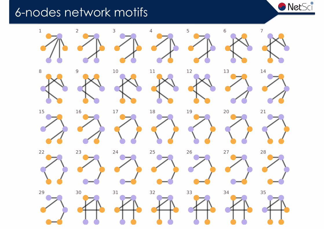
6-nodes network motifs
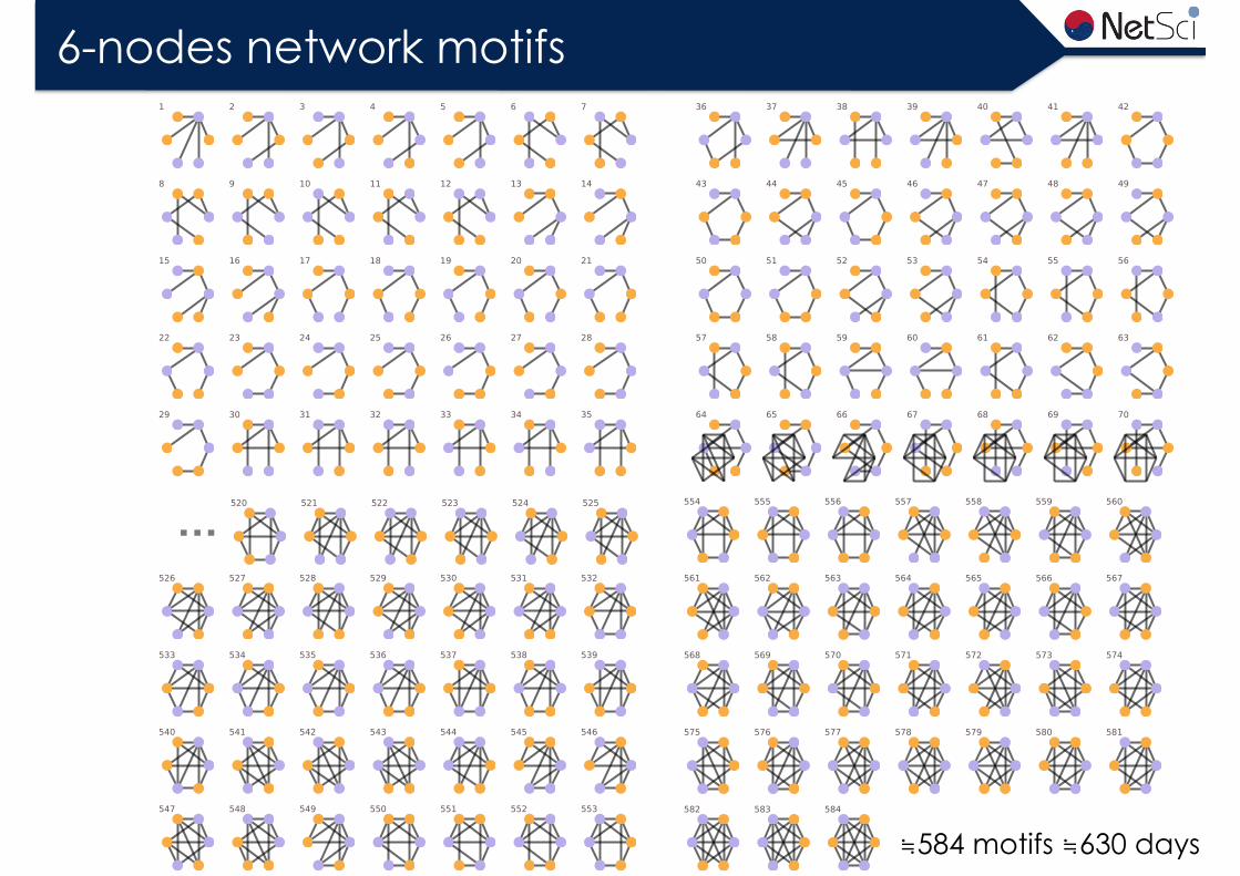
6-nodes network motifs
…
≒630 days≒584 motifs

3-points classification
0
1
0 50 100 150
Bas
in s
tab
ilit
y
K
BS of 2-nodes networks
Producer Consumer
0
1
0 20 40
Bas
in s
tab
ilit
y
K
BS of 4-nodes networks
ProducerConsumer
0
1
0 50 100 150
Bas
in s
tab
ilit
y
K
BS of 2-nodes networks
Producer Consumer
0
1
0 20 40
Bas
in s
tab
ilit
y
K
BS of 4-nodes networks
ProducerConsumer
0
1
0 10 20 30 40
Bas
inst
abil
ity
K
Node 1
Node 2 Node 3
Node 4
0
1
0 10 20 30 40
Bas
inst
abil
ity
K
Node 1
Node 2 Node 3
Node 4
0
1
0 10 20 30 40
Bas
inst
abil
ity
K
Node 1
Node 2 Node 3
Node 4
0
1
0 10 20 30 40
Bas
inst
abil
ity
K
Node 1
Node 2 Node 3
Node 4

3-points classification
0
1
0 50 100 150
Bas
in s
tab
ilit
y
K
BS of 2-nodes networks
Producer Consumer
0
1
0 20 40
Bas
in s
tab
ilit
y
K
BS of 4-nodes networks
ProducerConsumer
3-points classification
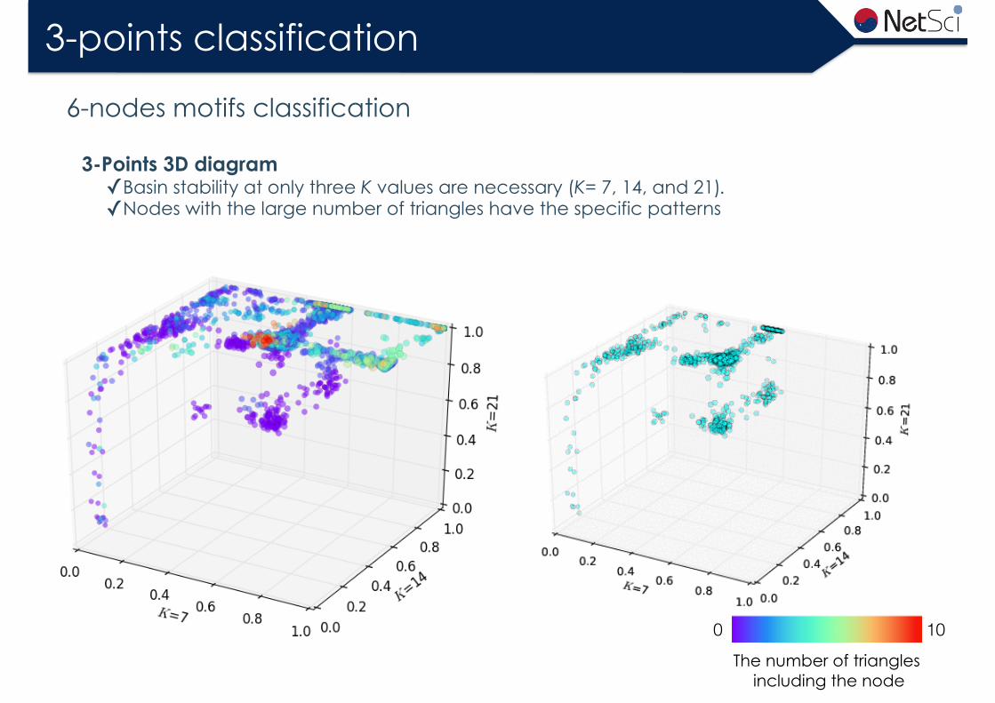
3-Points 3D diagram ✓Basin stability at only three K values are necessary (K= 7, 14, and 21). ✓Nodes with the large number of triangles have the specific patterns
6-nodes motifs classification
0 10The number of triangles
including the node

3-points classification
(b) (c)
(d) (e)
(a)

Result 2
0
1
0 10 20 30 40
Bas
inst
abil
ity
K
Node 1
Node 2 Node 3
Node 4
0
1
0 10 20 30 40
Bas
inst
abil
ity
K
Node 1
Node 2 Node 3
Node 40
1
0 10 20 30 40
Bas
inst
abil
ity
K
Node 1
Node 2 Node 3
Node 4
BS
K (BS>0.4)

Conclusion
Transition shape matters✓Basin stability measures synchronisation stability. ✓The transition pattern explains the synchronization
stability
✓Transition pattern of BS is affected by topology (structure of network and attributes of nodes). ✓Betweenness predicts the shape of patterns
✓Transition window is correlated with CC ✓Synchronization characteristics is correlated
with meso-scopic network characteristics
Transition window vs Community consistency
Transition patterns vs Betweenness
e5n1-1e4n2-1e3n2-2e3n2-1e2n1-0e1n2-0e1n2-1e1n1-1
e1n2-1
e1n2-0
e2n1-0
e3n2-1
e3n2-1
e3n2-1
e3n2-1
Bas
in s
tab
ilit
y
K
e1n1-1
0
0.5
1
0 20 40 60 80
Bas
in s
tab
ilit
y
K
Node a1
0
0.5
1
Node b1
0
0.5
1
0 50 100 150
(a) (b)
Node b2
How and why…?

Acknowledgement
Any postdoc position?
Petter Holme Heetae Kim Eun Lee Minjin LeeSang Hoon Lee
Now you can graduate!
National Research Foundation in Korea
H. Kim, S. H. Lee, P. Holme, New J. Phys. 17, 113005 (2015). H. Kim, S. H. Lee, P. Holme, arXiv:1602.01712 (2016)