06775257

948 IEEE TRANSACTIONS ON INFORMATION FORENSICS AND SECURITY, VOL. 9, NO. 6, JUNE 2014

A New Sketch Method for Measuring HostConnection Degree Distribution

Pinghui Wang, Xiaohong Guan, Fellow, IEEE, Junzhou Zhao, Jing Tao, and Tao Qin, Student Member, IEEE

Abstract— The host connection degree distribution (HCDD) isan important metric for network security monitoring. However,it is difficult to accurately obtain the HCDD in real time forhigh-speed links with a massive amount of traffic data. In thispaper, we propose a new sketch method to build a probabilistictraffic summary of a host’s flows using a uniform Flajolet–Martinsketch combined with a small bitmap. To study its performancein comparison with previous sampling and sketch methods, wepresent a general model that encompasses all these methods.With this model, we compute the Cramér–Rao lower boundsand the variances of HCDD estimations. The theoretic analysisand numerical experimental results show that our sketch methodis six times more accurate than state-of-the-art methods with thesame memory usage.

Index Terms— Network monitoring, traffic analysis.

I. INTRODUCTION

ALOT of research efforts have been made on measuringtraffic volume including heavy hitter detection [1]–[5],

heavy change detection [6]–[8], flow size distribution estima-tion [9]–[15], and traffic entropy estimation [16], [17]. Besidesthese statistics of traffic volumes, the host connection degreeis also an important indicator for network monitoring, wherea host’s connection degree is defined as the number of distincthosts that the host connects to. For example, super hostswith a large number of connections are usually caused bynetwork anomalies [18]–[21]. Moreover, Nychis et al. [22]observe that the host connection degree distribution (HCDD)is not consistent with other distributions, such as the hosttraffic volume distribution, and more likely to reflect networkanomalies. In fact the HCDD has been applied to applications

Manuscript received February 8, 2013; revised December 8, 2013 andFebruary 27, 2014; accepted March 6, 2014. Date of publication March19, 2014; date of current version April 30, 2014. This work was supportedin part by Xi’an Jiaotong University, in part by the National Natural Sci-ence Foundation of China under Grant 61103240, Grant 61103241, Grant61221063, and Grant 91118005, and in part by the Application FoundationResearch Program of SuZhou under Grant SYG201311. The associate editorcoordinating the review of this manuscript and approving it for publication wasProf. Wanlei Zhou.

P. Wang is with the Noah’s Ark Laboratory, Huawei Technologies,Hong Kong (e-mail: [email protected]).

X. Guan is with the MOE Key Laboratory for Intelligent Networks andNetwork Security, Xi’an Jiaotong University, Xi’an 710049, China, and alsowith the Center for Intelligent and Networked Systems, Tsinghua NationalLaboratory for Information Science and Technology, Tsinghua University,Beijing 100084, China (e-mail: [email protected]).

J. Zhao, J. Tao, and T. Qin are with the MOE Key Laboratory forIntelligent Networks and Network Security, Xi’an Jiaotong University,Xi’an 710049, China (e-mail: [email protected]; [email protected];[email protected]).

Color versions of one or more of the figures in this paper are availableonline at http://ieeexplore.ieee.org.

Digital Object Identifier 10.1109/TIFS.2014.2312544

for security monitoring, such as anomaly detection [23]–[28]and host profiling [29].

In this paper, we aim to measure the HCDD in realtimefor high speed links. Measuring traffic statistics has to beimplemented with very fast and expensive SRAM for realtimeapplications at routers, since DRAM does not support therequired high access rates. It is also critical for future softdefined networks. For example, Yu et al. [30] propose a trafficmeasurement architecture to deploy existing sketch methodson routers in software defined networks. To obtain the totalnumber of flows generated by a host, one needs to build a tablethat keeps track of existing flows to avoid duplicating flowrecords for packets from the same flow, where a flow refersto the set of packets with the same source and destination.Clearly it is not practical to obtain the connection degreesof all hosts by building per-host tables for high speed linkswith a large number of hosts and flows, since SRAM is anexpensive and scarce resource on routers. Therefore, it isvery important to design memory- and computation-efficientmethods for computing the HCDD of large networks.

Sampling technique provides a direct and efficient way toanalyze and process massive data, since only a relatively smallsubset of network traffic needs to be stored and processed.Similar to estimate flow size distribution [9], [11], one canestimate the HCDD using sampled traffic. Another is sketchesas in [31]–[35] to independently build a probabilistic summaryof flows per host using a small and fast memory, and then theconnection degree of a host can be estimated individually withits associated sketch. To accurately estimate the connectiondegree of a host with thousands of connections, these sketchmethods need to process an array of thousands of bits. Sincethe connection degree of a host is not known in advance, thetotal memory use is very large for a high speed link withmillions of hosts, and it limits the practical applications ofthe sketch methods in [31]–[35]. To solve this problem, thesketch methods in [18], [36], and [37] measure host connectiondegrees by building a very compact digest of monitored trafficfor all hosts, where the bitmaps used for estimating hostconnection degrees are not generated independently. Howeverthey fail to compute the HCDD, since the correlations ofthe bitmaps are too complex to analyze. Chen et al. [38]proposed a sketch method to measure the HCDD by building acontinuous uniform Flajolet-Martin sketch (CUFMS) for eachhost. The method uses a CUFMS to record the minimal orderstatistic of the hash values of a host’s flows, where the hashvalue of a flow is a random value selected from the range (0, 1)at random. The CUFMS of a host with more flows is smallerwith high probability, so the magnitude of a host’s CUFMS

1556-6013 © 2014 IEEE. Personal use is permitted, but republication/redistribution requires IEEE permission.See http://www.ieee.org/publications_standards/publications/rights/index.html for more information.

WANG et al.: NEW SKETCH METHOD FOR MEASURING HCDD 949

provides a measure for its connection degree. Based on thisproperty, the method in [38] estimate the HCDD using themaximum likelihood estimation method. However, we cannoteasily determine whether a host has a large connection degreefrom its CUFMS, since a small CUFMS might also begenerated by most hosts with small connection degrees. Thus,the estimation accuracy of the CUFMS method in [38] is aserious issue.

To address this problem, we present a joint sketch (JS)method. JS uses a discrete uniform Flajolet-Martin sketch(DUFMS) combined with a small bitmap [32] to build acompact digest of a host’s flows. DUFMS is the actualapplication version of the CUFMS, and the bitmap of a host isdefined as a bit array, where each bit is initialized with zero.For each flow of a host, a bit is randomly selected from thehost’s bitmap, and set as one. As a probabilistic summary, thenumber of ones in a host’s bitmap reflects the host’s connectiondegree. JS is more efficient and accurate than the CUFMSmethod because JS uses small bitmaps to build very accuratesketches for most hosts, since most hosts have several flowsand only a small fraction of hosts have thousands of flows.JS also builds a more effective traffic digest than the CUFMSmethod for hosts with a large number of flows, because allbits in the bitmap of a host with a large number of flowswill be set as one with high probability due to the “couponcollector’s problem” [39], and then the bitmap reflects that thehost’s connection degree is not smaller than L ln L, where Lis the size of the bitmap. To study the performance of JSin comparison with state-of-the-art methods, we propose ageneral model that encompasses all these methods. With thismodel, we compute the Cramér-Rao lower bounds and thevariances of HCDD estimations. The theoretic analysis andnumerical experimental results show that our method JS issignificantly more accurate than state-of-the-art methods withthe same memory usage. Meanwhile experiments based on realand simulated anomaly traffic show that JS is also efficient tomeasure the change of the HCDD, which is another importantindicator for detecting network anomalies.

This paper is organized as follows. The problem is formu-lated in Section II. In Section III we briefly discuss previousmethods and our sketch method for measuring the HCDD, andintroduce a general model that encompasses all these HCDDmeasurement methods. Section IV presents an efficient methodto compute the maximum likelihood estimation of the HCDD.Then we apply the information theory to study and analyzethe confidence interval of HCDD estimates in Section V. Theperformance evaluation and testing results are presented inSection VI. Section VII summarizes related work. Concludingremarks then follow.

II. PROBLEM FORMULATION

Let P = p1, p2, . . . be an input packet stream arrivingsequentially at a network monitor. Here pt = (st , dt ) refers tothe t-th packet, where st and dt are its source and destinationrespectively. We define the out-degree of a source s as thenumber of distinct destinations s connects to, and the in-degree of a destination d as the number of distinct sources

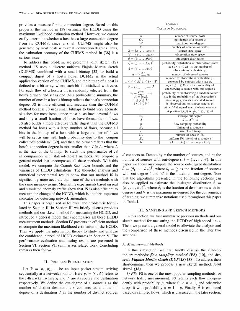
TABLE I

TABLE OF NOTATIONS

d connects to. Denote by n the number of sources, and ni thenumber of sources with out-degree i , i = {1, . . . , W }. In thispaper we focus on compute the source out-degree distribution�θ = (θ1, . . . , θW )T, where θi = ni

n is the fraction of sourceswith out-degree i and W is the maximum out-degree. Notethat the algorithms presented in the following sections canalso be applied to estimate the in-degree distribution �ϑ =(ϑ1, . . . , ϑV )T, where �ϑi is the fraction of destinations with in-degree i and V is the maximum in-degree. For the convenienceof reading, we summarize notations used throughout this paperin Table I.

III. SAMPLING AND SKETCH METHODS

In this section, we first summarize previous methods and oursketch method for measuring the HCDD of high speed links.Then, we present a general model to alleviate the analysis andthe comparison of these methods discussed in the later twosections.

A. Measurement Methods

In this subsection, we first briefly discuss the state-of-the-art methods: flow sampling method (FS) [10], and dis-crete Flajolet-Martin sketch (DUFMS) [38]. To address theirshortcomings, then we propose a new sketch method: jointsketch (JS).

1) FS: FS is one of the most popular sampling methods fornetwork traffic measurement. FS retains each flow indepen-dently with probability p, where 0 < p < 1, and otherwisedrops it with probability q = 1 − p. Finally, �θ is estimatedbased on sampled flows, which is discussed in the later section.


2) DUFMS: DUFMS can be viewed as an actual imple-mentation of the continuous Flajolet-Martin sketch (CUFMS)proposed in [38], which is a variant of a Flajolet-Martinsketch [31]. DUFMS uses a random variable Zs to build arough sketch for flows of a source s. Let Zs initialized with H .For an incoming packet (s, d), Zs is updated as

Zs = min{Zs, η(s||d)},where η is a uniform hash function with the range {1, . . . , H }and the flow label s||d is the concatenation of the source s andthe destination d . In a later subsection we show that the largerthe out-degree of s, the smaller Zs is with high probability.Thus, the magnitude of Zs reflects the out-degree of s. Basedon this property, �θ is estimated based on the sketches ofsampled sources, which is discussed later.

3) JS: To obtain an accurate estimate of �θ , [40] shows thatFS requires to set a large value of p. It makes FS memoryextensive. For CUFMS, we cannot easily determine whethera source s has a large out-degree from its zs , since the smallvalue of zs might also be generated by s with a small out-degree. Therefore the estimation accuracy of CUFMS is aserious issue. To solve this problem, we propose a new sketchmethod JS. JS uses a DUFMS Zs combined with a bitmapBs to build a probability traffic summary for a source s. Thebitmap Bs is defined as a bit array Bs[l], 1 ≤ l ≤ L, andeach bit Bs[l] is initialized with zero. For an incoming packet(s, d), we randomly select a bit from Bs and set it as one.That is, we update Bs as

Bs[ζ(s||d)] = 1,

where ζ(s||d) is a uniform hash function with therange {1, . . . , L}. Meanwhile we update Zs as Zs =min(Zs, η(s||d)), where Zs is initialized with H and η is auniform hash function with range {1, . . . , H }.

We observe that most sources’ out-degrees are small andonly a small fraction of sources have large out-degrees. Thus,JS using a small bitmap builds very accurate sketches for mostsources. For a source with a large out-degree, all bits in itsbitmap will be set as one with high probability due to the“coupon collector’s problem” [39], and then its bitmap reflectsthat its out-degree is not smaller than L ln L. Therefore, JScan also build a more effective traffic digest than DUFMS forsources with a large out-degree.

B. General Model

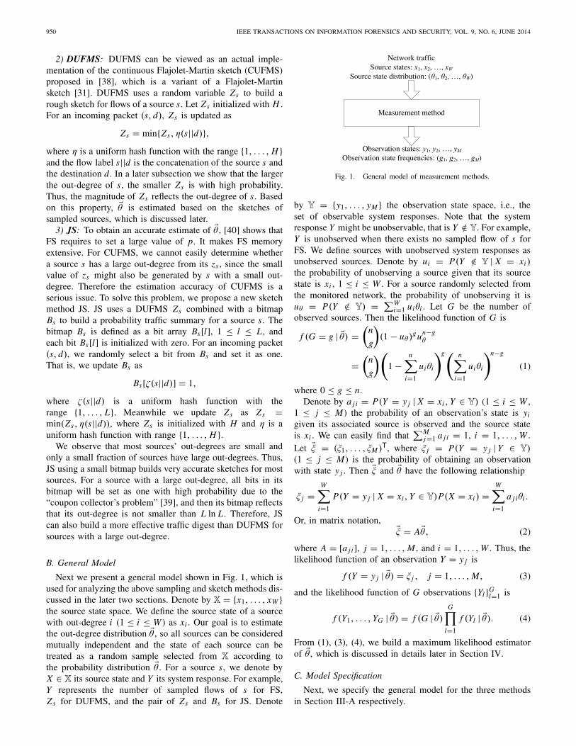
Next we present a general model shown in Fig. 1, which isused for analyzing the above sampling and sketch methods dis-cussed in the later two sections. Denote by X = {x1, . . . , xW }the source state space. We define the source state of a sourcewith out-degree i (1 ≤ i ≤ W ) as xi . Our goal is to estimatethe out-degree distribution �θ , so all sources can be consideredmutually independent and the state of each source can betreated as a random sample selected from X according tothe probability distribution �θ . For a source s, we denote byX ∈ X its source state and Y its system response. For example,Y represents the number of sampled flows of s for FS,Zs for DUFMS, and the pair of Zs and Bs for JS. Denote

Fig. 1. General model of measurement methods.

by Y = {y1, . . . , yM } the observation state space, i.e., theset of observable system responses. Note that the systemresponse Y might be unobservable, that is Y /∈ Y. For example,Y is unobserved when there exists no sampled flow of s forFS. We define sources with unobserved system responses asunobserved sources. Denote by ui = P(Y /∈ Y | X = xi )the probability of unobserving a source given that its sourcestate is xi , 1 ≤ i ≤ W . For a source randomly selected fromthe monitored network, the probability of unobserving it isuθ = P(Y /∈ Y) = ∑W

i=1 uiθi . Let G be the number ofobserved sources. Then the likelihood function of G is

f (G = g | �θ) =(

n

g

)

(1 − uθ )gun−g

θ

=(

n

g

) (

1 −n∑

i=1

uiθi

)g (n∑

i=1

uiθi

)n−g

(1)

where 0 ≤ g ≤ n.Denote by a j i = P(Y = y j | X = xi , Y ∈ Y) (1 ≤ i ≤ W ,

1 ≤ j ≤ M) the probability of an observation’s state is yi

given its associated source is observed and the source stateis xi . We can easily find that

∑Mj=1 a j i = 1, i = 1, . . . , W .

Let �ξ = (ξ1, . . . , ξM )T, where ξ j = P(Y = y j | Y ∈ Y)(1 ≤ j ≤ M) is the probability of obtaining an observationwith state y j . Then �ξ and �θ have the following relationship

ξ j =W∑

i=1

P(Y = y j | X = xi , Y ∈ Y)P(X = xi ) =W∑

i=1

a j iθi .

Or, in matrix notation,�ξ = A �θ, (2)

where A = [a j i], j = 1, . . . , M , and i = 1, . . . , W . Thus, thelikelihood function of an observation Y = y j is

f (Y = y j | �θ) = ξ j , j = 1, . . . , M, (3)

and the likelihood function of G observations {Yl}Gl=1 is

f (Y1, . . . , YG | �θ) = f (G | �θ)

G∏

l=1

f (Yl | �θ). (4)

From (1), (3), (4), we build a maximum likelihood estimatorof �θ , which is discussed in details later in Section IV.

C. Model Specification

Next, we specify the general model for the three methodsin Section III-A respectively.


1) FS: Denote by O ′s the number of sampled flows for a

source s. Then we have

P(O ′s = j | Os = i) =

(i

j

)

p j qi− j , 0 ≤ j ≤ i,

where Os is the out-degree of s. s is observed if and onlyif at least one of its flows is sampled, which happens withprobability P(O ′

s > 0) = 1 − q Os . Corresponding to thegeneral model, we have �ξ = (ξ1, . . . , ξW )T and A = [a j i ],j, i = 1, . . . , W , where a j i (1 ≤ j ≤ i ≤ W ) is the probabilityof observing j flows of a source with out-degree i , that is

a j i = P(O ′s = j | O ′

s > 0, Os = i) =( i

j

)p j qi− j

1 − qi.

Let a j i = 0 for i < j . We can easily find that the probabilityof unobserving a source with out-degree i is qi . Therefore, wehave ui = qi , and

uθ =W∑

i=1

qiθi . (5)

Thus, the probability that the number of sampled sourcesequals g (0 ≤ g ≤ n) is

f (G = g | �θ) =(

n

g

) (

1 −W∑

i=1

qiθi

)g (W∑

i=1

qiθi

)n−g

.

2) DUFMS: We can easily find that

P(Zs ≥ j | Os = i) =⎧⎨

⎩

(1 − j−1

H

)i, 1 ≤ j ≤ H

0, otherwise.

Then, the probability that Zs equals j is

a j i = P(Zs = j | Os = i)

= P(Zs ≥ j | Os = i) − P(Zs ≥ j + 1 | Os = i)

=(

1 − j − 1

H

)i

−(

1 − j

H

)i

. (6)

When the out-degree of s is large, (6) indicates that itsassociated Zs is small with high probability. Therefore themagnitude of Zs provides a measure for the out-degree ofs. Corresponding to the general model, we have A = [a j i ],j = 1, . . . , H , i = 1, . . . , W , and �ξ = (ξ1, . . . , ξH )T.

3) JS: Denote by Us the number of ones in Bs . Next wecompute the probability P(Us = j), 1 ≤ j ≤ L. For j distinctbits, there exist j !S(i, j) ways to partition i flows into thesebits given that each bit has at least one flow, where S(i, j),1 ≤ j ≤ i , the Stirling number of the second kind [41], iscomputed as

S(i, j) = 1

j !j−1∑

k=0

(−1)k(

j

k

)

( j − k)i , 1 ≤ j ≤ i.

Meanwhile, since there exist(L

j

)ways to select j distinct bits

from Bs , we have

P(Us = j | Os = i) =(L

j

)j !S(i, j)

Li

=(

L

j

) j−1∑

k=0

(−1)k(

j

k

) (j − k

L

)i

. (7)

Let j1 = 1, . . . , min{L, W }, and j2 = 1, . . . , H . Denotej = ( j1 − 1)H + j2. Corresponding to the general model, wedefine the observation state of s as Y = y j when Us = j1 andZs = j2. Then we have �ξ = (ξ1, . . . , ξM )T and A = [a j i], j =1, . . . , M , i = 1, . . . , W , where M = H min{L, W }, anda j i is computed as

a j i = P(Us = j1, Zs = j2 | Os = i)

= P(Us = j1 | Os = i)P(Zs = j2 | Os = i).

From (6) and (7), we have

a j i =(

L

j1

) j1−1∑

k=0

(−1)k(

j1k

) (j1 − k

L

)i

×((

1 − j2 − 1

H

)i

−(

1 − j2H

)i)

.

Let a j i = 0 for j1 > i .

IV. HCDD ESTIMATION METHOD

In this section, we present our maximum likelihood estima-tion (MLE) method to estimate the source out-degree distrib-ution �θ for the sampling and sketch methods in Section III-A.For the general model, denote by g j (1 ≤ j ≤ M) thenumber of observations with state y j , and g = ∑M

j=1 gi thenumber of observations. Let �g = (g1, . . . , gM)T. From (4),the log-likelihood function of observations with respect to theparameter �θ is computed as

L(�θ) = log f (G = g | �θ) +M∑

j=1

g j log f (Y = y j | �θ).

The MLE of �θ is defined as �θ = arg max�θ L(�θ). However itis hard to find a closed form solution to this optimization. Tosolve this problem, in what follows we study the complete-data likelihood function of observations with respect to �θ .Denote by f j i (1 ≤ j ≤ M , 1 ≤ i ≤ W ) the number ofobservations with state y j generated by sources with state xi ,and f0i the number of unobserved sources with state xi . Thenthe complete-data log-likelihood function is

Lc(�θ) =W∑

i=1

⎛

⎝ f0i log(uiθi ) +M∑

j=1

f j i log((1 − ui )a j iθi

)⎞

⎠ .

(8)To solve the optimization of �θ = arg maxθ Lc(�θ) with theconstrains

∑Wi=1 θi = 1 and 0 ≤ θi ≤ 1, the MLE of �θ is

computed as

θi =∑M

j=0 f j i∑W

i=1∑M

j=0 f j i.

Clearly f j i (0 ≤ j ≤ M , 1 ≤ i ≤ W ) are not directlyavailable. To solve this problem, we adopt a standardmethod, expectation maximization (EM) algorithm [42].Formally, EM begins with a guess of �θ(0), and is an iterativemethod which alternates between performing an expectationstep (E-step) and a maximization step (M-step). The k-th(k ≥ 0) iteration of these two steps is shown as follows:


E-step: Compute Q(�θ, �θ(k)), the expectation of thelog-likelihood evaluated using the current estimate �θ(k)

of �θ , as

Q(�θ, �θ(k)) =W∑

i=1

E �θ(k) [ f0i | �g] log(uiθi )

+W∑

i=1

M∑

j=1

E �θ(k) [ f j i | �g] log((1 − ui )a j iθi

).

which replaces f j i by their expectations E[ f j i ] given �θ(k)

in (8). Denote by pi | j (1 ≤ j ≤ M , 1 ≤ i ≤ W ) theprobability of an observation with state y j is generated bya source with state xi . We have

pi | j = P(

X = xi | Y = y j , �θ(k))

=P

(Y = y j | X = xi , Y ∈ Y, �θ(k)

)P

(X = xi | �θ(k)

)

P(

Y = y j | Y ∈ Y, �θ(k))

= a j iθ(k)i

∑Wl=1 a jlθ

(k)l

.

Thus,

E �θ(k) [ f j i | �g] = g j pi | j , 1 ≤ j ≤ M, 1 ≤ i ≤ W.

Denote by pi | 0 the probability that a system response isgenerated by a source with state xi given that the systemresponse is unobservable. Then we have

pi | 0 = P(

X = xi | Y /∈ Y, �θ(k))

= uiθ(k)i

∑Wl=1 ulθ

(k)l

.

Denote by g0 = n − g the number of unobserved sources. Ifn is known in advance, we have

E �θ(k) [ f0i | �g] = g0 pi | 0.

Otherwise, since

E �θ(k) [g0 | �g] = E �θ(k) [n]W∑

i=1

uiθ(k)i

= E �θ(k)

[g0 + g | �g] W∑

i=1

uiθ(k)i ,

we have

E �θ(k) [g0 | �g] = g∑W

i=1 uiθ(k)i

1 − ∑Wi=1 uiθ

(k)i

.

Thus,

E �θ(k) [ f0i | �g] = E �θ(k) [g0 | �g]pi | 0 = gpi | 0∑W

i=1 uiθ(k)i

1 − ∑Wi=1 uiθ

(k)i

.

M-step: Compute �θ(k+1) as the following equations that isthe value of �θ maximizing the expected log-likelihood foundon the E-step

θ(k+1)i =

∑Mj=0 g j pi | j

∑Wi=1

∑Mj=0 g j pi | j

, i = 1, . . . , W.

where g0 = n − g if n is known in advance, otherwise g0 =g

∑Wi=1 uiθ

(k)i

1−∑Wi=1 ui θ

(k)i

. We repeat these two steps multiple times until

�θ(k) and �θ(k+1) are close enough to each other.

V. ERROR ANALYSIS OF HCDD ESTIMATES

It is hard to directly analyze the variance of the MLE inSection IV. To solve this problem, in this section we computethe Cramér-Rao lower bound (CRLB) of �θ for the methodsin Section III-A. The CRLB of �θ provides a confidenceinterval of estimates given by the MLE, since the MLE is anasymptotically efficient unbiased estimator of �θ , and its meansquare error asymptotically approaches the CRLB of �θ [43].

A. CRLB of General Model

To compute the CRLB of �θ , in what follows we firstcompute the Fisher information of observations in respectto �θ . Then we obtain the CRLB of �θ assuming that �θ isunconstrained, i.e., θi ∈ R, i = 1, . . . , W , and

∑Wi=1 θi can

assume any value. However, �θ is a probability distribution(constrained), which should decrease the estimation error andconsequently the CRLB of �θ . Thus, later we see how to extendthis result to the case where �θ has the constraints:

∑Wi=1 θi = 1

and 0 < θi < 1, i = 1, . . . , W .The following closely follows the exposition in [44], which

estimates the flow size distribution from sampled packets. Foran observed source, its associated observation is a randomvariable distributed in the observation space Y = {y1, . . . , yM }according to the probability distribution �ξ = (ξ1, . . . , ξM )T.The unconstrained Fisher information of observations {Yl}G

l=1is a M × M matrix J = [Jik ], i, k = 1, . . . , W , where

Jik � E

[∂ ln f (Y1, . . . , YG | �θ)

∂θi

∂ ln f (Y1, . . . , YG | �θ)

∂θk

]

(9)

Since Yl is obtained independently, the likelihood functionf (Y1, . . . , YG | �θ) is computed as (4) and then we have

Theorem 1: J = [Jik ], i, k = 1, . . . , W , is computed as

Jik = E

[∂ ln f (G | �θ)

∂θi

∂ ln f (G | �θ)

∂θk

]

+E[G]E

[∂ ln f (Y | �θ)

∂θi

∂ ln f (Y | �θ)

∂θk

]

. (10)

Proof. From (4), we have

ln f (Y1, . . . , YG | �θ) = ln f (G | �θ) +G∑

l=1

ln f (Yl | �θ). (11)

Meanwhile,

E

[∂ ln f (G | �θ)

∂θi

]

= E

[∂ f (G | �θ)

∂θi

1

f (G | �θ)

]

=n∑

g=0

∂ f (G = g | �θ)

∂θi

= ∂

∂θi

n∑

g=0

f (G = g | �θ)

= 0. (12)


Similarly,

E

[∂ ln f (Yl | �θ)

∂θi

]

= 0, l = 1, . . . , G. (13)

From (9), (11), (12), and (13), we have (10). �The Fisher information matrix provides a lower bound on

the accuracy of estimators. Let �θ = (θ1, . . . , θW )T be anunbiased estimator of �θ . The Cramér-Rao Theorem statesthat the mean square error of any unbiased estimator θ j islower bounded by J−1 = [(J−1)ik ], i, k = 1, . . . , W , theinverse of the Fisher information matrix J , provided someweak regularity conditions [45, Ch. 2], i.e.,

E[θ j − θ j )2] ≥ (J−1) j j , 1 ≤ j ≤ W. (14)

The lower bound in (14) is known as the CRLB. Moreover,constraints on the estimated parameters provide information tothe estimator and can increase the Fisher information contentof samples. In [46], they find that only the equality constraint∑W

i=1 θi = 1 actually results in information gain. Denotematrix I = [Iik ], i, k = 1, . . . , W . Let

I = J−1 − J−1�o�oT J−1

�oT J−1�o , (15)

where �o = (1, . . . , 1)T is a vector with size W . Then we have

E[θ j − θ j )2] ≥ I j j , 1 ≤ j ≤ W.

B. Simplified Formulation of CRLB

Next, we simplify the CRLB formulations for the threemethods in Section III-A.

1) DUFMS and JS: DUFMS and JS sample sources withthe same probability, and then build sketches for sampledsources. Thus, f (G = g | �θ) is uncorrelated with �θ , i.e.,

∂ ln f (G = g | �θ)

∂θi= 0.

From (2) and (3), we have

∂ ln f (Y = y j | �θ)

∂θi= a j i

ξ j.

From Theorem 1, then we have

Jik = n(1 − uθ )

M∑

j=1

a j ia jk

ξ j.

Or, in matrix form,

J = n(1 − uθ )AT�A,

where � is a M×M diagonal matrix whose element at location( j, j) is 1

ξ j, 1 ≤ j ≤ M . Denote J = AT�A. Then we have

J = n(1 − uθ ) J .

Therefore, J−1 is computed as

J−1 = J−1

n(1 − uθ ).

Moreover, we have J−1�o�oT J−1 = �θ �θT, and �oT J−1�o = 1from [47]. Thus, we simplify (15) as

I = J−1 − �θ �θT

n(1 − uθ ). (16)

2) FS: We have the following equation from (1)

∂ ln f (G = g | �θ)

∂θi= (n(1 − uθ ) − g)ui

uθ (1 − uθ ).

Thus, we have

E

[∂ ln f (G | �θ)

∂θi

∂ ln f (G | �θ)

∂θk

]

=n∑

g=0

(n(1 − uθ ) − g)2ui uk

(uθ (1 − uθ ))2 f (G = g | �θ)

= nui uk

uθ (1 − uθ ).

From Theorem 1, then we have

Jik = nui uk

uθ (1 − uθ )+ n(1 − uθ )

M∑

j=1

a j ia jk

ξ j.

Or, in matrix form,

J = n�u �uT

uθ (1 − uθ )+ n(1 − uθ ) J .

When uθ (1 − uθ )2 + �uT J−1�u �= 0, J−1 is computed as the

following equation by the matrix inversion lemma [48]

J−1 = 1

n(1 − uθ )

(

J−1 − J−1�u�uT J−1

uθ (1 − uθ )2 + �uT J−1�u

)

.

VI. EXPERIMENTS

In this section, we first conduct experiments to study theCRLB of JS in comparison with state-of-the-art methods. Thenwe compute the errors of HCDD estimates given by the MLE.Finally we show results of measuring HCDDs’ changes fornetwork anomaly detection.

A. Datasets

We evaluate our method based on two public packet headertraces [49]. These two traces are obtained from the actualnetwork traffic over the backbones of CERNET (China Edu-cation and Research Network) as gathered at the NorthwestRegional Center. Trace 1 is collected at a 10 Gbps linkby using TCPDUMP for about ten minutes. It consists of2.1 × 108 packet headers, and includes 2.1 × 105 sources and8.2 × 105 flows. Trace 2 is collected at an egress router witha bandwidth of 1.5 Gbps for about eleven hours. It consistsof 5.8 × 108 packet headers, and includes 1.7 × 106 sourcesand 7.0 × 106 flows. To evaluate our method for detectingabnormal traffic, we also conduct experiments based on thewitty worm dataset [50].


TABLE II

SPACE COMPLEXITIES OF FS, DUFMS, AND JS

TABLE III

COMPUTATIONAL COMPLEXITIES OF FS, DUFMS, AND JS FOR

UPDATING A SAMPLED PACKET (RUNNING TIME IS CALCULATED BY

PERFORMING EXPERIMENTS ON A 2.39 GHZ INTEL PROCESSOR)

B. Comparison Model

In this subsection we give a model to compare FS,DUFMS, and JS. From (5), we find that n(1 − ∑W

i=1 qiθi )sources are expected to be sampled for FS with samplingprobability p. To store the information of sampled flows, wehave two different schemes: the computation efficient schemeFS_C and the memory efficient scheme FS_M. FS_C directlyadopts a flow table to store the labels of sampled flows.Therefore, on average its memory use is 64npmθ bits. FS_Mallocates a destination table for a sampled source. Then itneeds 32 + 32t bits for a source with t flows sampled, andits average memory use is 32n(pmθ + 1 − ∑W

i=1 qiθi ) bits.Therefore, FS_M is more memory efficient at the cost ofmore computations. Denote by nD and n J the numbers ofsources sampled by DUFMS and JS respectively. Then thespace complexities of FS, DUFMS, and JS are shown inTable II. Table III shows the computational complexities ofFS_C, FS_M, DUFMS, and JS. For a sampled packet, we usea hash table to determine whether its associated flow appearedpreviously for FS_C and FS_M. Similar, hash tables are usedto store data summaries of sampled sources for DUFMS andJS. The average computational complexities are all O(1) forthese four methods. We conduct experiments on a 2.39 GHzIntel processor running Windows XP. We observe that asampled packet is processed very efficiently, which is less thanone microsecond for all these four methods. In the followingexperiments FS, DUFMS, and JS are compared under thesame memory usage, that is achieved by setting p, nD , and n J .

C. Accuracy of Estimating the HCDD

In this subsection, we compute the CRLB and the error ofestimates given by the MLE to evaluate the performance ofJS in comparison with FS and DUFMS respectively.

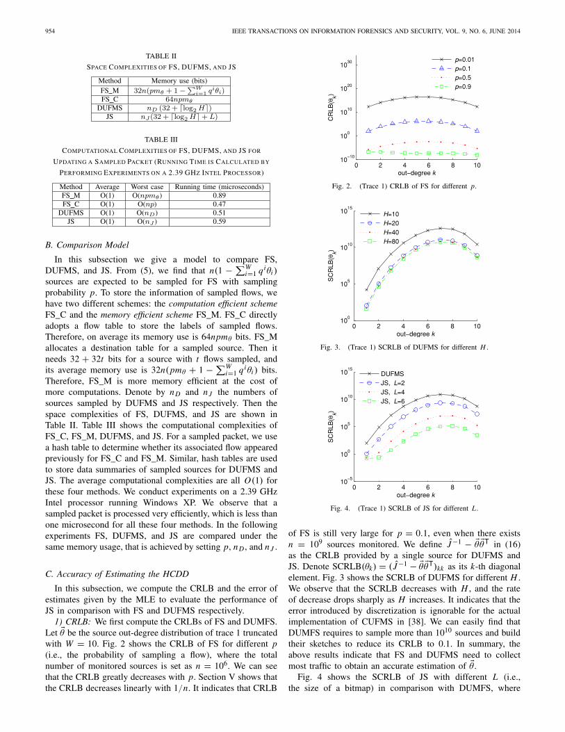
1) CRLB: We first compute the CRLBs of FS and DUMFS.Let �θ be the source out-degree distribution of trace 1 truncatedwith W = 10. Fig. 2 shows the CRLB of FS for different p(i.e., the probability of sampling a flow), where the totalnumber of monitored sources is set as n = 106. We can seethat the CRLB greatly decreases with p. Section V shows thatthe CRLB decreases linearly with 1/n. It indicates that CRLB

Fig. 2. (Trace 1) CRLB of FS for different p.

Fig. 3. (Trace 1) SCRLB of DUFMS for different H .

Fig. 4. (Trace 1) SCRLB of JS for different L .

of FS is still very large for p = 0.1, even when there existsn = 109 sources monitored. We define J−1 − �θ �θT in (16)as the CRLB provided by a single source for DUFMS andJS. Denote SCRLB(θk) = ( J−1 − �θ �θT)kk as its k-th diagonalelement. Fig. 3 shows the SCRLB of DUFMS for different H .We observe that the SCRLB decreases with H , and the rateof decrease drops sharply as H increases. It indicates that theerror introduced by discretization is ignorable for the actualimplementation of CUFMS in [38]. We can easily find thatDUMFS requires to sample more than 1010 sources and buildtheir sketches to reduce its CRLB to 0.1. In summary, theabove results indicate that FS and DUFMS need to collectmost traffic to obtain an accurate estimation of �θ .

Fig. 4 shows the SCRLB of JS with different L (i.e.,the size of a bitmap) in comparison with DUMFS, where


Fig. 5. SCRLB of DUFMS for different �θ .

Fig. 6. SCRLB of JS for different �θ .

Fig. 7. The CRLB of JS in comparison with the MSE of MLE estimates.

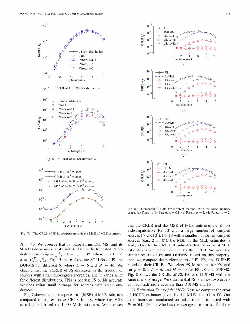
H = 40. We observe that JS outperforms DUFMS, and itsSCRLB decreases sharply with L. Define the truncated Paretodistribution as θk = α

σkα+1 , k = 1, . . . , W , where α > 0 and

σ = ∑Wk=1

αkα+1 . Figs. 5 and 6 show the SCRLBs of JS and

DUFMS for different �θ , where L = 6 and H = 40. Weobserve that the SCRLB of JS decreases as the fraction ofsources with small out-degrees increases, and it varies a lotfor different distributions. This is because JS builds accuratesketches using small bitmaps for sources with small out-degrees.

Fig. 7 shows the mean square error (MSE) of MLE estimatescompared to its respective CRLB for JS, where the MSEis calculated based on 1,000 MLE estimates. We can see

Fig. 8. Compared CRLBs for different methods with the same memoryusage. (a) Trace 1. (b) Pareto, α = 0.1. (c) Pareto, α = 1. (d) Pareto, α = 2.

that the CRLB and the MSE of MLE estimates are almostindistinguishable for JS with a large number of sampledsources (≥ 2×105). For JS with a smaller number of sampledsources (e.g., 2 × 104), the MSE of the MLE estimates isfairly close to the CRLB. It indicates that the error of MLEestimates is accurately bounded by the CRLB. We omit thesimilar results of FS and DUFMS. Based on this property,then we compare the performances of JS, FS, and DUFMSbased on their CRLBs. We select FS_M scheme for FS, andset p = 0.1, L = 6, and H = 40 for FS, JS and DUFMS.Fig. 8 shows the CRLBs of JS, FS, and DUFMS with thesame memory usage. We observe that JS is almost two ordersof magnitude more accurate than DUFMS and FS.

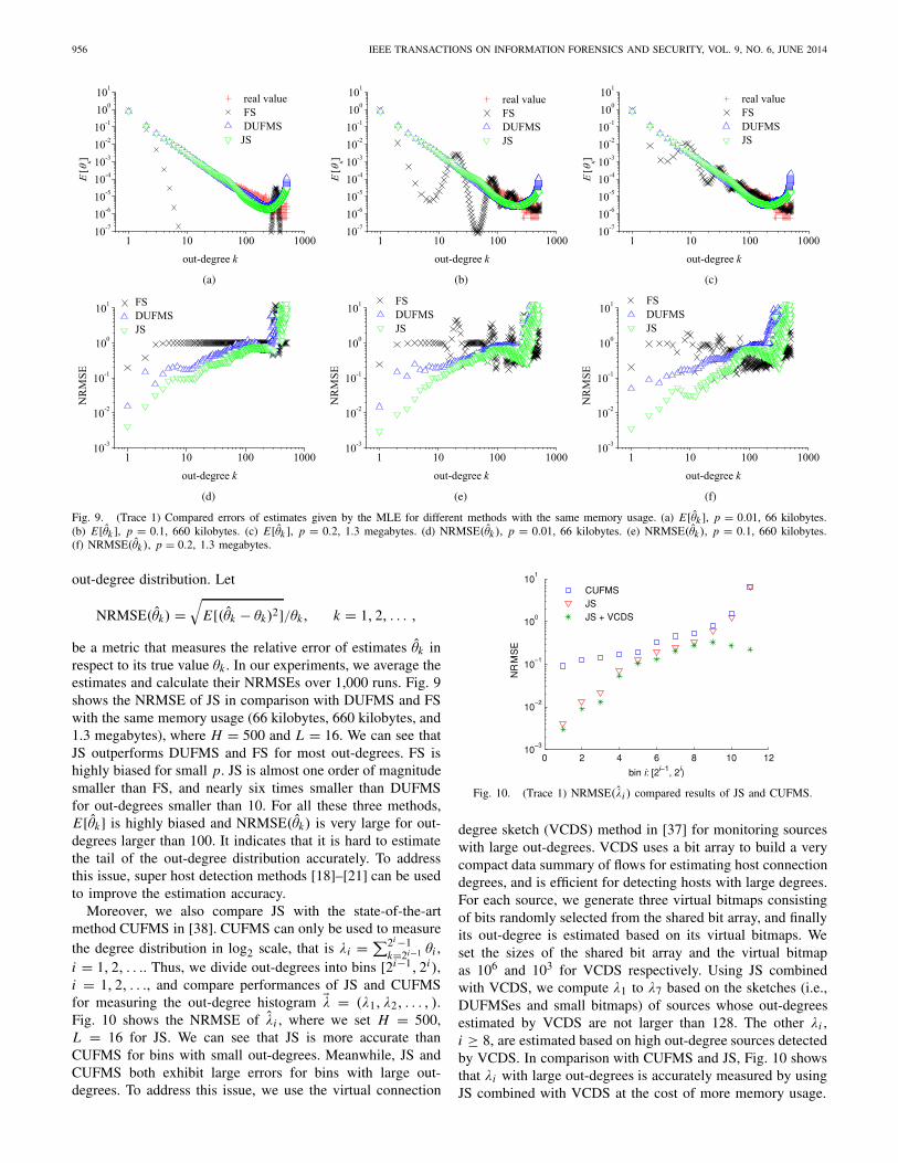
2) Estimation Error of the MLE: Next we compute the errorof HCDD estimates given by the MLE method in IV. Ourexperiments are conducted on traffic trace 1 truncated withW = 500. Denote E[θk] as the average of estimates θk of the


Fig. 9. (Trace 1) Compared errors of estimates given by the MLE for different methods with the same memory usage. (a) E[θk ], p = 0.01, 66 kilobytes.(b) E[θk ], p = 0.1, 660 kilobytes. (c) E[θk ], p = 0.2, 1.3 megabytes. (d) NRMSE(θk ), p = 0.01, 66 kilobytes. (e) NRMSE(θk), p = 0.1, 660 kilobytes.(f) NRMSE(θk ), p = 0.2, 1.3 megabytes.

out-degree distribution. Let

NRMSE(θk) =√

E[(θk − θk)2]/θk, k = 1, 2, . . . ,

be a metric that measures the relative error of estimates θk inrespect to its true value θk . In our experiments, we average theestimates and calculate their NRMSEs over 1,000 runs. Fig. 9shows the NRMSE of JS in comparison with DUFMS and FSwith the same memory usage (66 kilobytes, 660 kilobytes, and1.3 megabytes), where H = 500 and L = 16. We can see thatJS outperforms DUFMS and FS for most out-degrees. FS ishighly biased for small p. JS is almost one order of magnitudesmaller than FS, and nearly six times smaller than DUFMSfor out-degrees smaller than 10. For all these three methods,E[θk] is highly biased and NRMSE(θk) is very large for out-degrees larger than 100. It indicates that it is hard to estimatethe tail of the out-degree distribution accurately. To addressthis issue, super host detection methods [18]–[21] can be usedto improve the estimation accuracy.

Moreover, we also compare JS with the state-of-the-artmethod CUFMS in [38]. CUFMS can only be used to measurethe degree distribution in log2 scale, that is λi = ∑2i −1

k=2i−1 θi ,i = 1, 2, . . .. Thus, we divide out-degrees into bins [2i−1, 2i ),i = 1, 2, . . ., and compare performances of JS and CUFMSfor measuring the out-degree histogram �λ = (λ1, λ2, . . . , ).Fig. 10 shows the NRMSE of λi , where we set H = 500,L = 16 for JS. We can see that JS is more accurate thanCUFMS for bins with small out-degrees. Meanwhile, JS andCUFMS both exhibit large errors for bins with large out-degrees. To address this issue, we use the virtual connection

Fig. 10. (Trace 1) NRMSE(λi ) compared results of JS and CUFMS.

degree sketch (VCDS) method in [37] for monitoring sourceswith large out-degrees. VCDS uses a bit array to build a verycompact data summary of flows for estimating host connectiondegrees, and is efficient for detecting hosts with large degrees.For each source, we generate three virtual bitmaps consistingof bits randomly selected from the shared bit array, and finallyits out-degree is estimated based on its virtual bitmaps. Weset the sizes of the shared bit array and the virtual bitmapas 106 and 103 for VCDS respectively. Using JS combinedwith VCDS, we compute λ1 to λ7 based on the sketches (i.e.,DUFMSes and small bitmaps) of sources whose out-degreesestimated by VCDS are not larger than 128. The other λi ,i ≥ 8, are estimated based on high out-degree sources detectedby VCDS. In comparison with CUFMS and JS, Fig. 10 showsthat λi with large out-degrees is accurately measured by usingJS combined with VCDS at the cost of more memory usage.


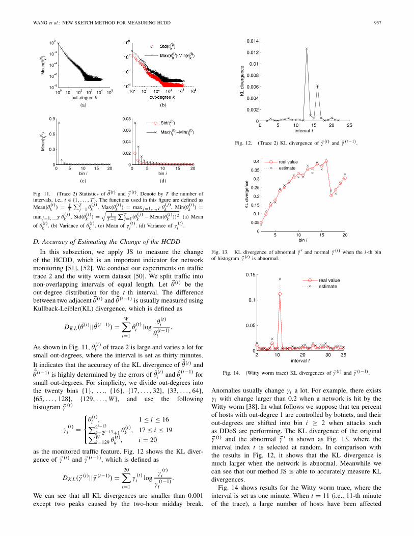
Fig. 11. (Trace 2) Statistics of �θ(t) and �γ (t). Denote by T the number ofintervals, i.e., t ∈ {1, . . . , T }. The functions used in this figure are defined asMean(θ

(t)k ) = 1

T∑T

j=1 θ( j)k , Max(θ

(t)k ) = max j=1,...,T θ

( j)k , Min(θ

(t)k ) =

min j=1,...,T θ( j)k , Std(θ

(t)k ) =

√1

T −1∑T

j=1(θ( j)k − Mean(θ

(t)k ))2. (a) Mean

of θ(t)k . (b) Variance of θ

(t)k . (c) Mean of γ

(t)i . (d) Variance of γ

(t)i .

D. Accuracy of Estimating the Change of the HCDD

In this subsection, we apply JS to measure the changeof the HCDD, which is an important indicator for networkmonitoring [51], [52]. We conduct our experiments on traffictrace 2 and the witty worm dataset [50]. We split traffic intonon-overlapping intervals of equal length. Let �θ(t) be theout-degree distribution for the t-th interval. The differencebetween two adjacent �θ(t) and �θ(t−1) is usually measured usingKullback-Leibler(KL) divergence, which is defined as

DK L(�θ(t)|| �θ(t−1)) =W∑

i=1

θ(t)i log

θ(t)i

θ(t−1)i

.

As shown in Fig. 11, θ(t)i of trace 2 is large and varies a lot for

small out-degrees, where the interval is set as thirty minutes.

It indicates that the accuracy of the KL divergence of �θ(t) and�θ(t−1) is highly determined by the errors of θ

(t)i and θ

(t−1)i for

small out-degrees. For simplicity, we divide out-degrees intothe twenty bins {1}, . . ., {16}, {17, . . . , 32}, {33, . . . , 64},{65, . . . , 128}, {129, . . . , W }, and use the followinghistogram �γ (t)

γ(t)i =

⎧⎪⎨

⎪⎩

θ(t)i , 1 ≤ i ≤ 16

∑2i−12

k=2i−13+1 θ(t)k , 17 ≤ i ≤ 19

∑Wk=129 θ

(t)k , i = 20

as the monitored traffic feature. Fig. 12 shows the KL diver-gence of �γ (t) and �γ (t−1), which is defined as

DK L( �γ (t)|| �γ (t−1)) =20∑

i=1

γ(t)i log

γ(t)i

γ(t−1)i

.

We can see that all KL divergences are smaller than 0.001except two peaks caused by the two-hour midday break.

Fig. 12. (Trace 2) KL divergence of �γ (t) and �γ (t−1).

Fig. 13. KL divergence of abnormal �γ ′ and normal �γ (t) when the i-th binof histogram �γ (t) is abnormal.

Fig. 14. (Witty worm trace) KL divergences of �γ (t) and �γ (t−1).

Anomalies usually change γi a lot. For example, there existsγi with change larger than 0.2 when a network is hit by theWitty worm [38]. In what follows we suppose that ten percentof hosts with out-degree 1 are controlled by botnets, and theirout-degrees are shifted into bin i ≥ 2 when attacks suchas DDoS are performing. The KL divergence of the original�γ (t) and the abnormal �γ ′ is shown as Fig. 13, where theinterval index t is selected at random. In comparison withthe results in Fig. 12, it shows that the KL divergence ismuch larger when the network is abnormal. Meanwhile wecan see that our method JS is able to accurately measure KLdivergences.

Fig. 14 shows results for the Witty worm trace, where theinterval is set as one minute. When t = 11 (i.e., 11-th minuteof the trace), a large number of hosts have been affected


Fig. 15. (Witty worm trace) Results of CUSUM.

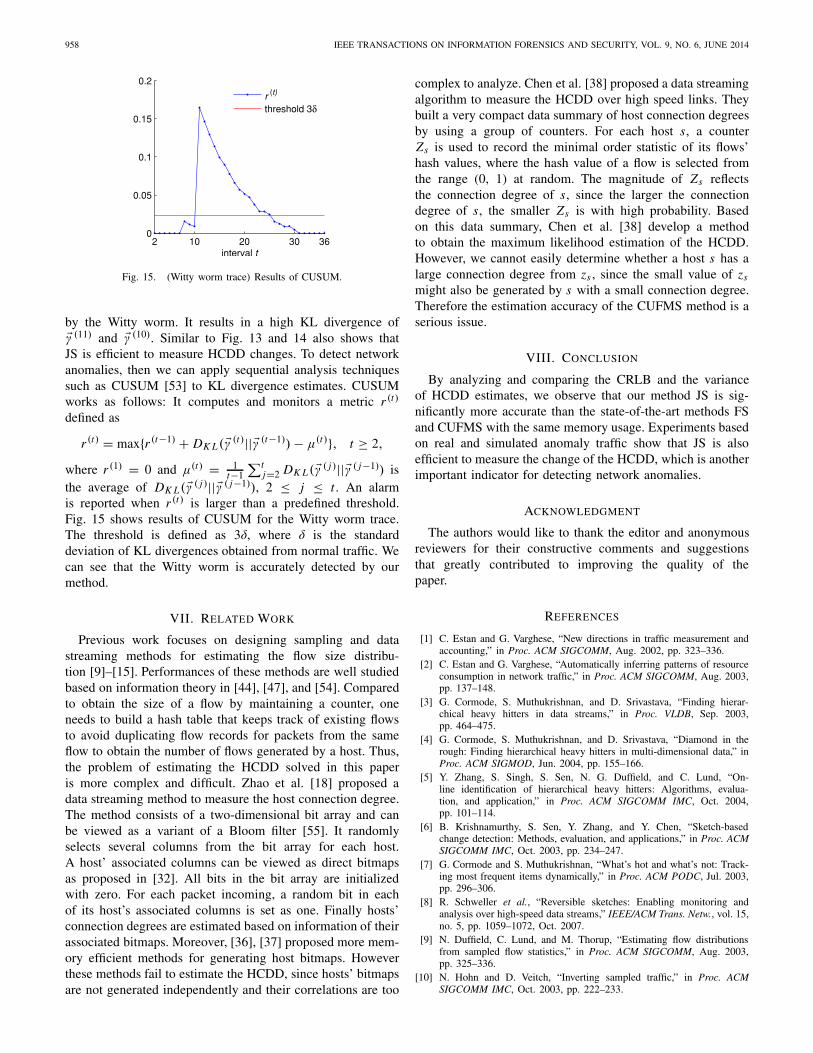
by the Witty worm. It results in a high KL divergence of�γ (11) and �γ (10). Similar to Fig. 13 and 14 also shows thatJS is efficient to measure HCDD changes. To detect networkanomalies, then we can apply sequential analysis techniquessuch as CUSUM [53] to KL divergence estimates. CUSUMworks as follows: It computes and monitors a metric r (t)

defined as

r (t) = max{r (t−1) + DK L( �γ (t)|| �γ (t−1)) − μ(t)}, t ≥ 2,

where r (1) = 0 and μ(t) = 1t−1

∑tj=2 DK L( �γ ( j )|| �γ ( j−1)) is

the average of DK L( �γ ( j )|| �γ ( j−1)), 2 ≤ j ≤ t . An alarmis reported when r (t) is larger than a predefined threshold.Fig. 15 shows results of CUSUM for the Witty worm trace.The threshold is defined as 3δ, where δ is the standarddeviation of KL divergences obtained from normal traffic. Wecan see that the Witty worm is accurately detected by ourmethod.

VII. RELATED WORK

Previous work focuses on designing sampling and datastreaming methods for estimating the flow size distribu-tion [9]–[15]. Performances of these methods are well studiedbased on information theory in [44], [47], and [54]. Comparedto obtain the size of a flow by maintaining a counter, oneneeds to build a hash table that keeps track of existing flowsto avoid duplicating flow records for packets from the sameflow to obtain the number of flows generated by a host. Thus,the problem of estimating the HCDD solved in this paperis more complex and difficult. Zhao et al. [18] proposed adata streaming method to measure the host connection degree.The method consists of a two-dimensional bit array and canbe viewed as a variant of a Bloom filter [55]. It randomlyselects several columns from the bit array for each host.A host’ associated columns can be viewed as direct bitmapsas proposed in [32]. All bits in the bit array are initializedwith zero. For each packet incoming, a random bit in eachof its host’s associated columns is set as one. Finally hosts’connection degrees are estimated based on information of theirassociated bitmaps. Moreover, [36], [37] proposed more mem-ory efficient methods for generating host bitmaps. Howeverthese methods fail to estimate the HCDD, since hosts’ bitmapsare not generated independently and their correlations are too

complex to analyze. Chen et al. [38] proposed a data streamingalgorithm to measure the HCDD over high speed links. Theybuilt a very compact data summary of host connection degreesby using a group of counters. For each host s, a counterZs is used to record the minimal order statistic of its flows’hash values, where the hash value of a flow is selected fromthe range (0, 1) at random. The magnitude of Zs reflectsthe connection degree of s, since the larger the connectiondegree of s, the smaller Zs is with high probability. Basedon this data summary, Chen et al. [38] develop a methodto obtain the maximum likelihood estimation of the HCDD.However, we cannot easily determine whether a host s has alarge connection degree from zs , since the small value of zs

might also be generated by s with a small connection degree.Therefore the estimation accuracy of the CUFMS method is aserious issue.

VIII. CONCLUSION

By analyzing and comparing the CRLB and the varianceof HCDD estimates, we observe that our method JS is sig-nificantly more accurate than the state-of-the-art methods FSand CUFMS with the same memory usage. Experiments basedon real and simulated anomaly traffic show that JS is alsoefficient to measure the change of the HCDD, which is anotherimportant indicator for detecting network anomalies.

ACKNOWLEDGMENT

The authors would like to thank the editor and anonymousreviewers for their constructive comments and suggestionsthat greatly contributed to improving the quality of thepaper.

REFERENCES

[1] C. Estan and G. Varghese, “New directions in traffic measurement andaccounting,” in Proc. ACM SIGCOMM, Aug. 2002, pp. 323–336.

[2] C. Estan and G. Varghese, “Automatically inferring patterns of resourceconsumption in network traffic,” in Proc. ACM SIGCOMM, Aug. 2003,pp. 137–148.

[3] G. Cormode, S. Muthukrishnan, and D. Srivastava, “Finding hierar-chical heavy hitters in data streams,” in Proc. VLDB, Sep. 2003,pp. 464–475.

[4] G. Cormode, S. Muthukrishnan, and D. Srivastava, “Diamond in therough: Finding hierarchical heavy hitters in multi-dimensional data,” inProc. ACM SIGMOD, Jun. 2004, pp. 155–166.

[5] Y. Zhang, S. Singh, S. Sen, N. G. Duffield, and C. Lund, “On-line identification of hierarchical heavy hitters: Algorithms, evalua-tion, and application,” in Proc. ACM SIGCOMM IMC, Oct. 2004,pp. 101–114.

[6] B. Krishnamurthy, S. Sen, Y. Zhang, and Y. Chen, “Sketch-basedchange detection: Methods, evaluation, and applications,” in Proc. ACMSIGCOMM IMC, Oct. 2003, pp. 234–247.

[7] G. Cormode and S. Muthukrishnan, “What’s hot and what’s not: Track-ing most frequent items dynamically,” in Proc. ACM PODC, Jul. 2003,pp. 296–306.

[8] R. Schweller et al., “Reversible sketches: Enabling monitoring andanalysis over high-speed data streams,” IEEE/ACM Trans. Netw., vol. 15,no. 5, pp. 1059–1072, Oct. 2007.

[9] N. Duffield, C. Lund, and M. Thorup, “Estimating flow distributionsfrom sampled flow statistics,” in Proc. ACM SIGCOMM, Aug. 2003,pp. 325–336.

[10] N. Hohn and D. Veitch, “Inverting sampled traffic,” in Proc. ACMSIGCOMM IMC, Oct. 2003, pp. 222–233.


[11] L. Yang and G. Michailidis, “Sample based estimation of networktraffic flow characteristics,” in Proc. IEEE INFOCOM, May 2007,pp. 1775–1783.

[12] A. Kumar, M. Sung, J. Xu, and J. Wang, “Data streaming algorithmsfor efficient and accurate estimation of flow size distribution,” in Proc.ACM SIGMETRICS, Jun. 2004, pp. 177–188.

[13] B. Ribeiro, T. Ye, and D. Towsley, “A resource-minimalist flow sizehistogram estimator,” in Proc. ACM SIGCOMM IMC, Oct. 2008,pp. 285–290.

[14] A. Kumar, M. Sung, J. Xu, and E. W. Zegura, “A data streamingalgorithm for estimating subpopulation flow size distribution,” in Proc.ACM SIGMETRICS, Jun. 2005, pp. 61–72.

[15] A. Kumar and J. Xu, “Sketch guided sampling–using online estimatesof flow size for adaptive data collection,” in Proc. IEEE INFOCOM,Apr. 2006, pp. 1–11.

[16] A. Lall, V. Sekar, M. Ogihara, J. Xu, and H. Zhang, “Data streamingalgorithms for estimating entropy of network traffic,” in Proc. ACMSIGMETRICS, Jun. 2006, pp. 145–156.

[17] H. Zhao, A. Lall, O. Spatscheck, J. Wang, and J. Xu, “A data streamingalgorithm for estimating entropies of OD flows,” in Proc. ACM SIG-COMM IMC, Oct. 2007, pp. 279–290.

[18] Q. Zhao, A. Kumar, and J. Xu, “Joint data streaming and samplingtechniques for detection of super sources and destinations,” in Proc.ACM SIGCOMM IMC, Oct. 2005, pp. 77–90.

[19] S. Venkataraman, D. Song, P. B. Gibbons, and A. Blum, “New stream-ing algorithms for fast detection of superspreaders,” in Proc. NDSS,Feb. 2005, pp. 149–166.

[20] J. Cao, Y. Jin, A. Chen, T. Bu, and Z. Zhang, “Identifying high cardinal-ity Internet hosts,” in Proc. IEEE INFOCOM, Apr. 2009, pp. 810–818.

[21] T. Li, S. Chen, W. Luo, and M. Zhang, “Scan detection in high-speed networks based on optimal dynamic bit sharing,” in Proc. IEEEINFOCOM, Apr. 2011, pp. 3200–3208.

[22] G. Nychis, V. Sekar, D. G. Andersen, H. Kim, and H. Zhang, “Anempirical evaluation of entropy-based traffic anomaly detection,” inProc. ACM SIGCOMM IMC, Oct. 2008, pp. 151–156.

[23] W. Lee and D. Xiang, “Information-theoretic measures for anom-aly detection,” in Proc. IEEE Symp. Security Privacy, May 2001,pp. 130–143.

[24] L. Feinstein, D. Schnackenberg, R. Balupari, and D. Kindred, “Statisticalapproaches to DDoS attack detection and response,” in Proc. DARPA Inf.Survivability Conf. Exposit., Apr. 2003, pp. 303–314.

[25] A. Lakhina, M. Crovella, and C. Diot, “Mining anomalies usingtraffic feature distributions,” in Proc. ACM SIGCOMM, Aug. 2005,pp. 217–228.

[26] A. Wagner and B. Plattner, “Entropy based worm and anomaly detectionin fast IP networks,” in Proc. 14th IEEE Int. Workshops EnablingTechnol., Infrastruct. Collaborative Enterprise, Jun. 2005, pp. 172–177.

[27] P. Wang, X. Guan, T. Qin, and Q. Huang, “A data streamingmethod for monitoring host connection degrees of high-speed links,”IEEE Trans. Inf. Forensics Security, vol. 6, no. 3, pp. 1086–1098,Sep. 2011.

[28] P. Wang, X. Guan, D. Towsley, and J. Tao, “Virtual indexing based meth-ods for estimating node connection degrees,” Comput. Netw., vol. 56,no. 12, pp. 2773–2787, 2012.

[29] K. Xu, Z.-L. Zhang, and S. Bhattacharyya, “Profiling Internet backbonetraffic: Behavior models and applications,” in Proc. ACM SIGCOMM,Aug. 2005, pp. 169–180.

[30] M. Yu, L. Jose, and R. Miao, “Software defined traffic measurement withopensketch,” in Proc. 10th USENIX Conf. Netw. Syst. Des. Implement.,Berkeley, CA, USA, 2013, pp. 29–42.

[31] P. Flajolet and N. G. Martin, “Probabilistic counting algorithms for database applications,” J. Comput. Syst. Sci., vol. 31, no. 2, pp. 182–209,Sep. 1985.

[32] K. Whang, B. T. Vander-zanden, and H. M. Taylor, “A linear-timeprobabilistic counting algorithm for database applications,” IEEE Trans.Database Syst., vol. 15, no. 2, pp. 208–229, Jun. 1990.

[33] M. Durand and P. Flajolet, “Loglog counting of large cardinalities,” inProc. Eur. Symp. Algorithms, Sep. 2003, pp. 605–617.

[34] C. Estan, G. Varghese, and M. Fisk, “Bitmap algorithms for countingactive flows on high speed links,” in Proc. ACM SIGCOMM IMC,Oct. 2003, pp. 182–209.

[35] A. Chen and J. Cao, “Distinct counting with a self-learning bitmap,” inProc. IEEE ICDE, Mar. 2009, pp. 1171–1174.

[36] M. Yoon, T. Li, S. Chen, and J. K. Peir, “Fit a spread estimator in smallmemory,” in Proc. IEEE INFOCOM, Apr. 2009, pp. 504–512.

[37] P. Wang, X. Guan, W. Gong, and D. Towsley, “A new virtual index-ing method for measuring host connection degrees,” in Proc. IEEEINFOCOM Mini-Conf., Apr. 2011, pp. 156–160.

[38] A. Chen, L. Li, and J. Cao, “Tracking cardinality distributions in networktraffic,” in Proc. IEEE INFOCOM, Apr. 2009, pp. 819–827.

[39] T. Motwani and P. Raghavan, Randomized Algorithms. New York, NY,USA: Cambridge Univ. Press, 1995.

[40] F. Murai, B. F. Ribeiro, D. Towsley, and P. Wang, “On set sizedistribution estimation and the characterization of large networks viasampling,” IEEE J. Sel. Areas Commun., vol. 31, no. 6, pp. 1017–1025,Jun. 2013.

[41] M. Abramowitz and I. A. Stegun, Handbook of Mathematical Functionswith Formulas, Graphs, and Mathematical Tables. Washington, DC,USA: NBS, 1972.

[42] A. P. Dempster, N. M. Laird, and D. B. Rubin, “Maximum likelihoodfrom incomplete data via the EM algorithm,” J. R. Statist. Soc., Ser. B(Methodol.), vol. 39, no. 1, pp. 1–38, 1977.

[43] P. J. Bickel and K. A. Doksum, Mathematical Statistics: Basic Ideas andSelected Topics, vol. 1, 2nd ed. Englewood Cliffs, NJ, USA: Prentice-Hall, 2000.

[44] B. Ribeiro, D. Towsley, T. Ye, and J. Bolot, “Fisher information ofsampled packets: An application to flow size estimation,” in Proc. ACMSIGCOMM IMC, Oct. 2006, pp. 15–26.

[45] H. L. van Trees, Detection, Estimation and Modulation Theory, Part 1.New York, NY, USA: Wiley, 2001.

[46] J. D. Gorman and A. O. Hero, “Lower bounds for parametric estimationwith constraints,” IEEE Trans. Inf. Theory, vol. 26, no. 6, pp. 1285–1301,Nov. 1990.

[47] P. Tune and D. Veitch, “Towards optimal sampling for flow sizeestimation,” in Proc. ACM SIGCOMM IMC, Oct. 2008, pp. 243–256.

[48] F. Zhang, Matrix Theory: Basic Results and Techniques. New York, NY,USA: Springer-Verlag, 1999.

[49] (2009, Sep. 1). Virtual Index Methods: Public Data Set [Online].Available: http://nskeylab.xjtu.edu.cn/people/phwang/data/

[50] (2013, Dec. 1). The CAIDA Witty Worm Dataset. [Online]. Available:http://www.caida.org/data/passive/witty_worm_dataset.xml

[51] Y. Gu, A. McCallum, and D. Towsley, “Detecting anomalies in networktraffic using maximum entropy estimation,” in Proc. ACM SIGCOMMIMC, Oct. 2005, pp. 345–350.

[52] M. P. Stoecklin, J.-Y. L. Boudec, and A. Kind, “A two-layered anom-aly detection technique based on multi-modal flow behavior mod-els,” in Proc. 9th Int. Conf. Passive Active Netw. Meas., Apr. 2008,pp. 212–221.

[53] E. S. Page, “Continuous inspection schemes,” Biometrika, vol. 41,nos. 1–2, pp. 100–115, Jun. 1954.

[54] P. Tune and D. Veitch, “Fisher information in flow size distributionestimation,” in Proc. IEEE INFOCOM, Apr. 2011, pp. 2105–2113.

[55] B. H. Bloom, “Space/time trade-offs in hash coding with allowableerrors,” Commun. ACM, vol. 13, no. 7, pp. 422–426, Jul. 1970.

Pinghui Wang received the B.S. degree in infor-mation engineering and the Ph.D. degree in auto-matic control from Xi’an Jiaotong University, Xi’an,China, in 2006 and 2012, respectively. In 2012, hewas a Post-Doctoral Researcher with the Departmentof Computer Science and Engineering, Chinese Uni-versity of Hong Kong, and the School of ComputerScience, McGill University, Montreal, QC, Canada,from 2012 to 2013. He is currently a Researcherwith Noah’s Ark Laboratory, Huawei Technologies,Hong Kong. His research interests include Internet

traffic measurement and modeling, traffic classification, abnormal detection,and online social network measurement.


Xiaohong Guan (S’89–M’93–SM’94–F’07) re-ceived the B.S. and M.S. degrees in automatic con-trol from Tsinghua University, Beijing, China, andthe Ph.D. degree in electrical engineering from theUniversity of Connecticut, Storrs, CT, USA, in 1982,1985, and 1993, respectively.

From 1993 to 1995, he was a Consulting Engi-neer at PG&E. From 1985 to 1988, he was withthe Systems Engineering Institute, Xi’an JiaotongUniversity, Xi’an, China, and the Division of En-gineering and Applied Science, Harvard University,

Cambridge, MA, USA, from 1999 to 2000. Since 1995, he has been with theSystems Engineering Institute, Xi’an Jiaotong University, and was a CheungKong Professor of Systems Engineering in 1999 and the Dean of the Schoolof Electronic and Information Engineering in 2008. Since 2001, he has beenthe Director of the Center for Intelligent and Networked Systems, TsinghuaUniversity, and served as the Head of the Department of Automation from2003 to 2008. He is an Editor of the IEEE TRANSACTIONS ON POWER

SYSTEMS and an Associate Editor of Automata. His research interests includeallocation and scheduling of complex networked resources, network security,and sensor networks.

Junzhou Zhao received the B.S. and M.S. degreesin information engineering from Xi’an Jiaotong Uni-versity, Xi’an, China, in 2008 and 2010, respectively,where he is currently pursuing the Ph.D. degreewith the Systems Engineering Institute and SKLMSLaboratory under the supervision of Prof. XiaohongGuan. His research interests include Internet trafficmeasurement and modeling, traffic classification,abnormal detection, and online social network mea-surement.

Jing Tao received the B.S. and M.S. degrees inautomation engineering from Xi’an Jiaotong Univer-sity, Xi’an, China, in 2001 and 2006, respectively,where he is currently a Teacher and pursuing an on-the-job Ph.D. degree with the Systems EngineeringInstitute and SKLMS Laboratory under the supervi-sion of Prof. Xiaohong Guan. His research interestsinclude Internet traffic measurement and modeling,traffic classification, abnormal detection, and botnet.

Tao Qin (S’08) received the B.S. and Ph.D. degreesin information engineering from Xi’an Jiaotong Uni-versity, Xi’an, China, in 2004 and 2010, respec-tively, where he is currently an Assistant Professorwith the Department of Computer Science. His re-search interests include Internet traffic measurementand modeling, traffic classification, and abnormaldetection.

Education

06775257