Welcome

Submitted To Dr. S. D. Solanki,Assistant Professor ,Dept. of Genetics & Plant BreedingC.P.C.A,S.D.A.U., Sardarkrushinagar.

Submitted BySatish M. KhadiaPh. D. , 6th sem., Dept. of Genetics & Plant BreedingC.P.C.A,S.D.A.U., Sardarkrushinagar.

Course: GP 504 : Quantitative Genetics

An Assignment on

Analysis of Variance (ANOVA), MANOVA: Expected variance components, Random and fixed models

Introduction• Variance: Average of the squares of deviations of the observations of a

sample from the mean of the sample drown from a population [ ∑(x – x)2/N]• Variance: The square of the standard deviation.

• The statistical procedure which separate or split the total variation into different components is known as “ANOVA”

• R.A. Fisher• “It is the technique of sorting out the total variation into some known and

unknown component of variation from a given set of data” Recognized source of variance are replication, genotype, error and total. It is a mathematical procedure of partitioning the total variation into

various recognized source of variance

Main Advantage

• Estimation of Components of Variance

• Provide basis for the test of significance

Aims of ANOVA

To sort out total variance and there by to estimate variance components.

To evaluate the hereditary contribution in a genetically problem.

To test predetermined hypothesis.

Scope of ANOVA

• Treatment study.

• Gives scope to understand treatment comparison.

• Gives idea of the magnetite of uncontrolled variation.

• It helps in future planning of experiment.

• It can be controlled by adopting principle of experimental design.

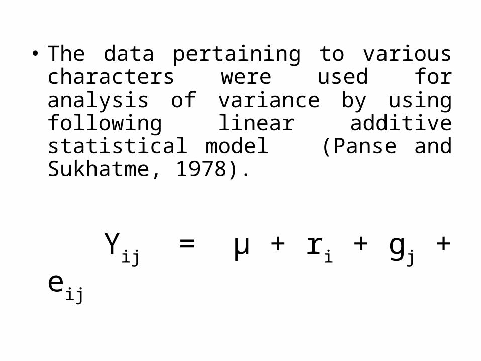
• The data pertaining to various characters were used for analysis of variance by using following linear additive statistical model (Panse and Sukhatme, 1978).

Yij = µ + ri + gj + eij

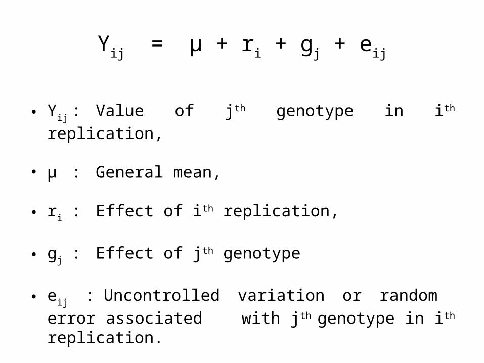
• Yij : Value of jth genotype in ith replication,

• µ : General mean,

• ri : Effect of ith replication,

• gj : Effect of jth genotype

• eij : Uncontrolled variation or random error associated with jth genotype in ith replication.

Yij = µ + ri + gj + eij

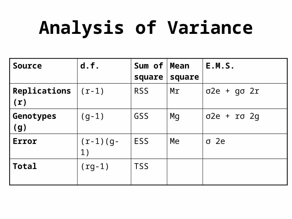
Analysis of Variance

Source d.f. Sum of square

Mean square

E.M.S.

Replications (r) (r-1) RSS Mr σ2e + gσ 2r

Genotypes (g) (g-1) GSS Mg σ2e + rσ 2g

Error (r-1)(g-1) ESS Me σ 2e

Total (rg-1) TSS

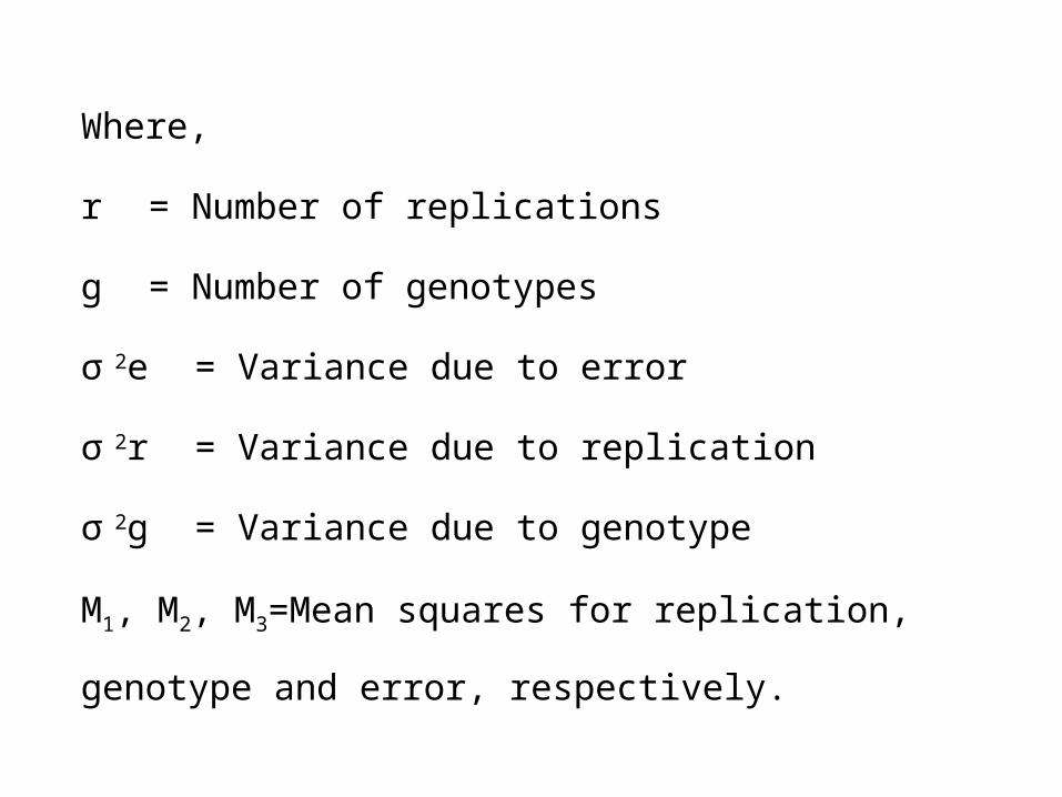
Where,

r = Number of replications

g = Number of genotypes

σ 2e = Variance due to error

σ 2r = Variance due to replication

σ 2g = Variance due to genotype

M1, M2, M3=Mean squares for replication, genotype

and error, respectively.

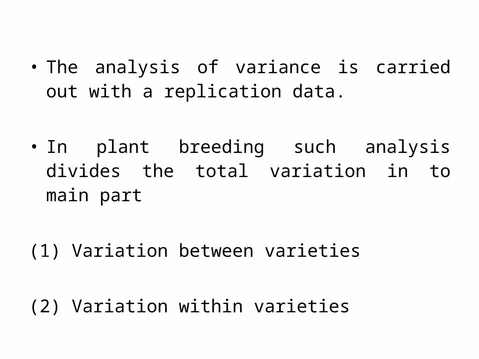
• The analysis of variance is carried out with a replication data.

• In plant breeding such analysis divides the total variation in to main part

(1) Variation between varieties

(2) Variation within varieties

Variance Components

• Genotypic variance (σ 2g)

• Phenotypic variance (σ 2p)

• Error variance (σ 2e)

1. Genotypic variance (σ 2g)

• The genotypic variance contributed by genetic causes or the occurrence of differences among individuals due to differences in their genetic make-up. It was calculated as under:

• Genotypic variance (σ 2g) = Mg – Me -------- rWhere, σ 2g = Genotypic variance,Mg = Genotypic mean square of the character,Me = Error mean square of the character, andr = Number of replications.

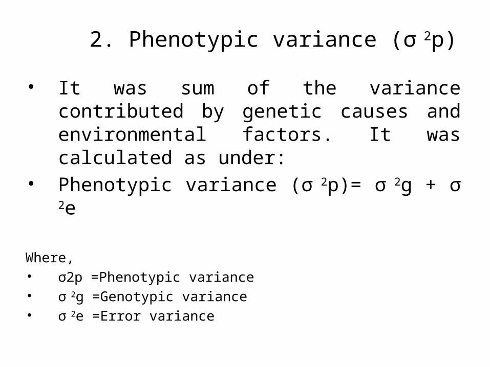
2. Phenotypic variance (σ 2p)

• It was sum of the variance contributed by genetic causes and environmental factors. It was calculated as under:

• Phenotypic variance (σ 2p)= σ 2g + σ 2e Where, • σ2p =Phenotypic variance• σ 2g =Genotypic variance• σ 2e =Error variance

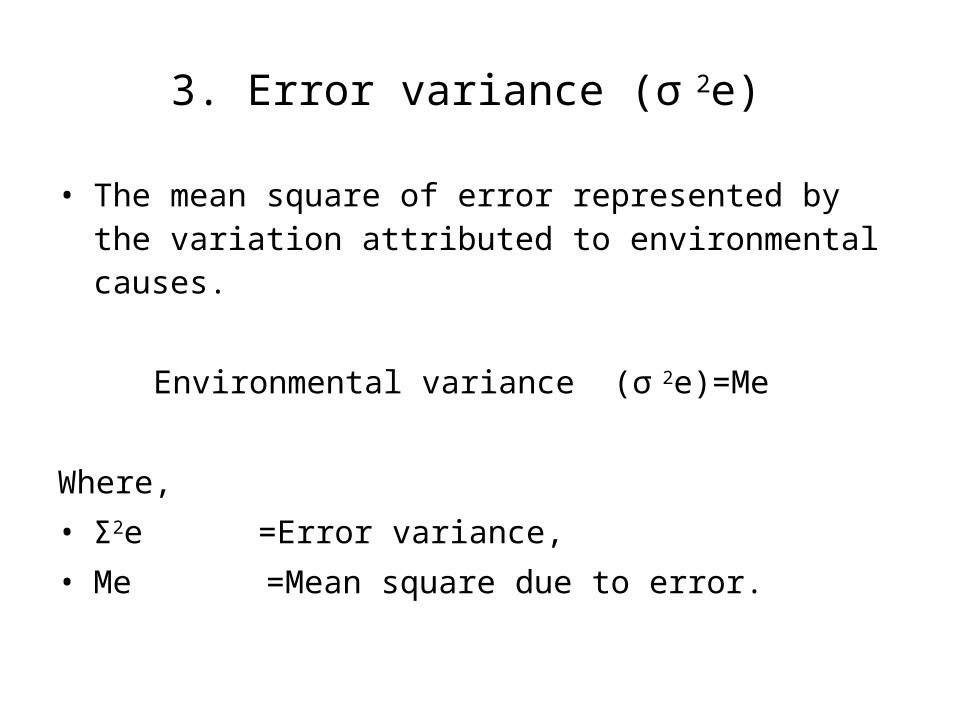
3. Error variance (σ 2e)

• The mean square of error represented by the variation attributed to environmental causes.

Environmental variance (σ 2e)=Me

Where, • Σ2e =Error variance, • Me =Mean square due to error.

Coefficient of Variance

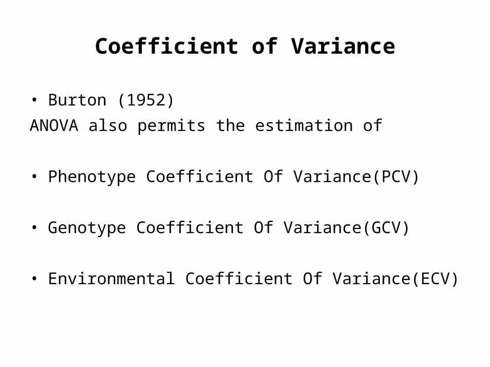
• Burton (1952)ANOVA also permits the estimation of • Phenotype Coefficient Of Variance(PCV)

• Genotype Coefficient Of Variance(GCV)

• Environmental Coefficient Of Variance(ECV)

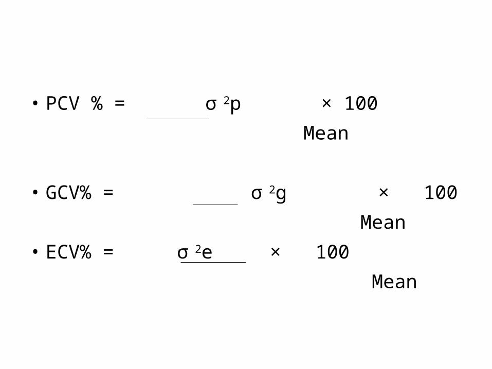
• PCV % = σ 2p × 100 Mean

• GCV% = σ 2g × 100 Mean• ECV% = σ 2e × 100 Mean

• PCV and GCV are classified for suggested by • Shivsubramanium and Madhavmenon (1973) Low : Less than 10% Moderate : 10-20% High : More than 20%

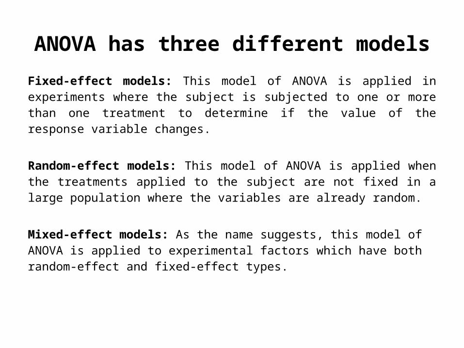
ANOVA has three different models

Fixed-effect models: This model of ANOVA is applied in experiments where the subject is subjected to one or more than one treatment to determine if the value of the response variable changes.

Random-effect models: This model of ANOVA is applied when the treatments applied to the subject are not fixed in a large population where the variables are already random.

Mixed-effect models: As the name suggests, this model of ANOVA is applied to experimental factors which have both random-effect and fixed-effect types.

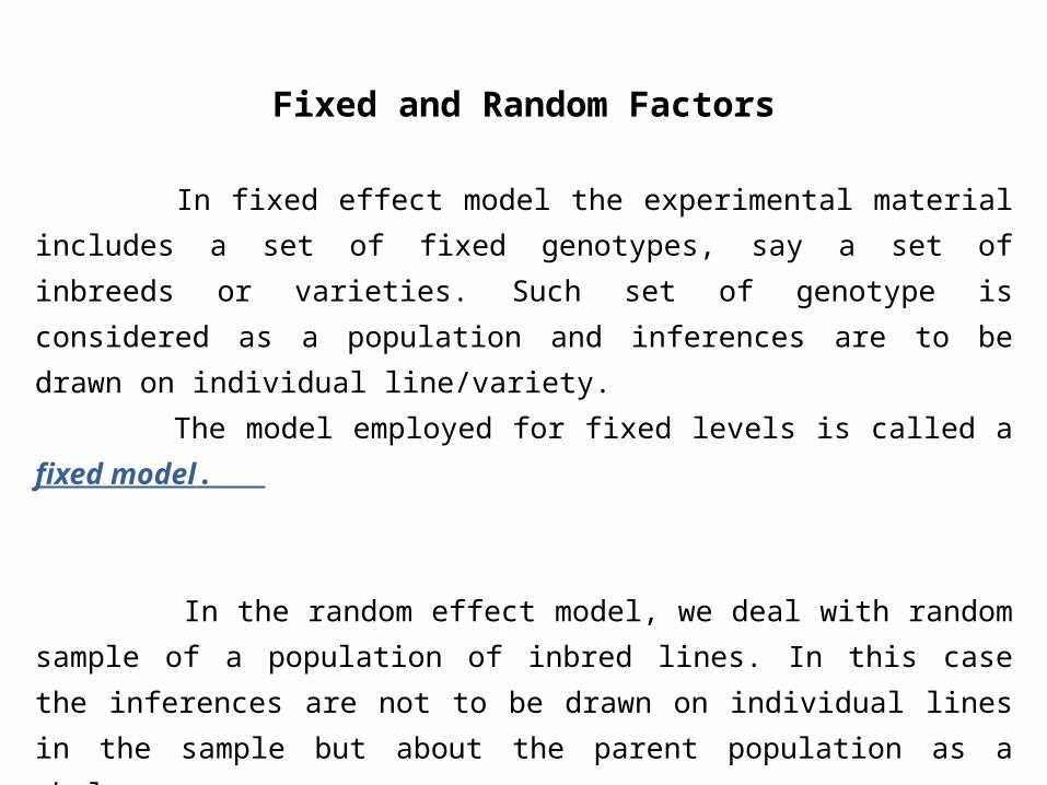
Fixed and Random Factors In fixed effect model the experimental material includes a set of fixed genotypes, say a set of inbreeds or varieties. Such set of genotype is considered as a population and inferences are to be drawn on individual line/variety. The model employed for fixed levels is called a fixed model.

In the random effect model, we deal with random sample of a population of inbred lines. In this case the inferences are not to be drawn on individual lines in the sample but about the parent population as a whole. Model is called a random model

Properties of random effects

• To illustrate some of the properties of random effects, suppose you collected data on the amount of insect damage to different varieties of wheat.

• It is impractical to study insect damage for every possible variety of wheat, so to conduct the experiment, you randomly select four varieties of wheat to study.

• Plant damage is rated for up to a maximum of four plots per variety. Ratings are on a 0 (no damage) to 10 (great damage) scale.

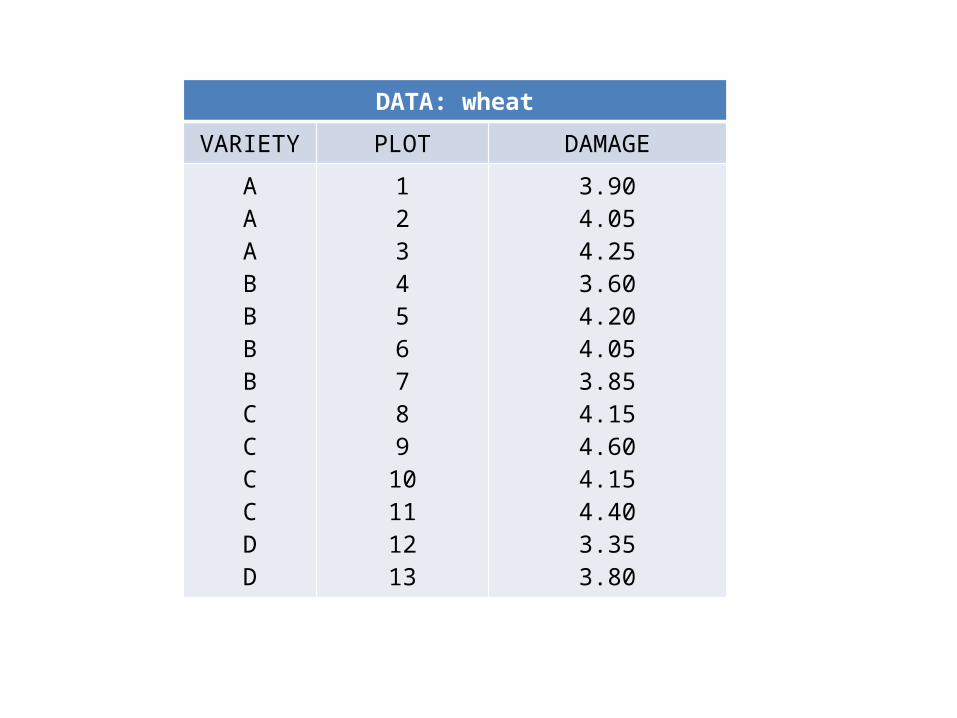
DATA: wheatVARIETY PLOT DAMAGE

AAABBBBCCCCDD

12345678910111213

3.904.054.253.604.204.053.854.154.604.154.403.353.80

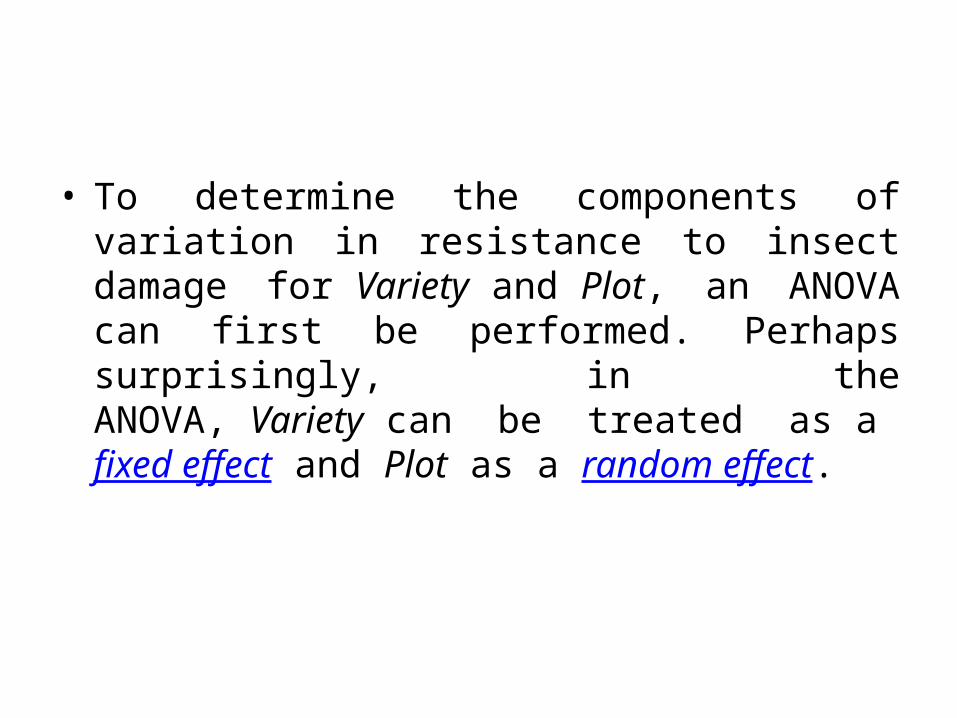
• To determine the components of variation in resistance to insect damage for Variety and Plot, an ANOVA can first be performed. Perhaps surprisingly, in the ANOVA, Variety can be treated as a fixed effect and Plot as a random effect.

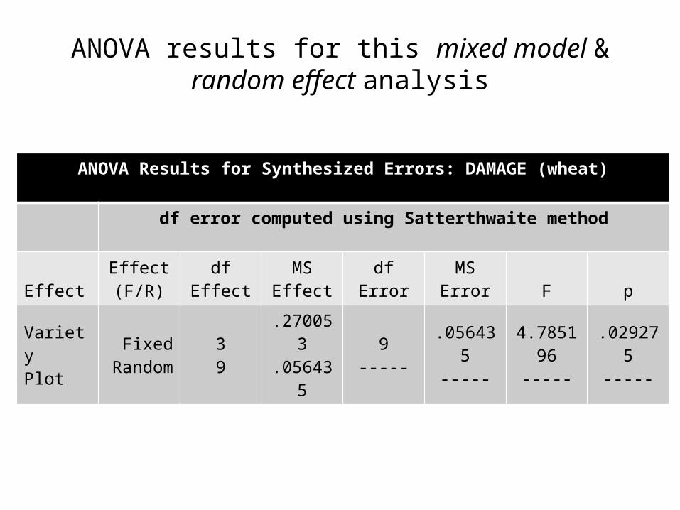
ANOVA results for this mixed model & random effect analysis

ANOVA Results for Synthesized Errors: DAMAGE (wheat)

df error computed using Satterthwaite method

EffectEffect(F/R)

dfEffect

MSEffect

dfError

MSError

 F

 p

VarietyPlot

FixedRandom

39

.270053

.0564359

-----.056435

-----4.785196

-----.029275

-----

• The difference in the two sets of estimates is that a variance component is estimated for Variety only when it is considered to be a random effect.

• This reflects the basic distinction between fixed and random effects.

• The variation in the levels of random factors is assumed to be representative of the variation of the whole population of possible levels.

• Thus, variation in the levels of a random factor can be used to estimate the population variation.

• Thus, the variation of a fixed factor cannot be used to estimate its population variance, nor can the population covariance with the dependent variable be meaningfully estimated.

Multivariate Analysis of Variance (MANOVA)

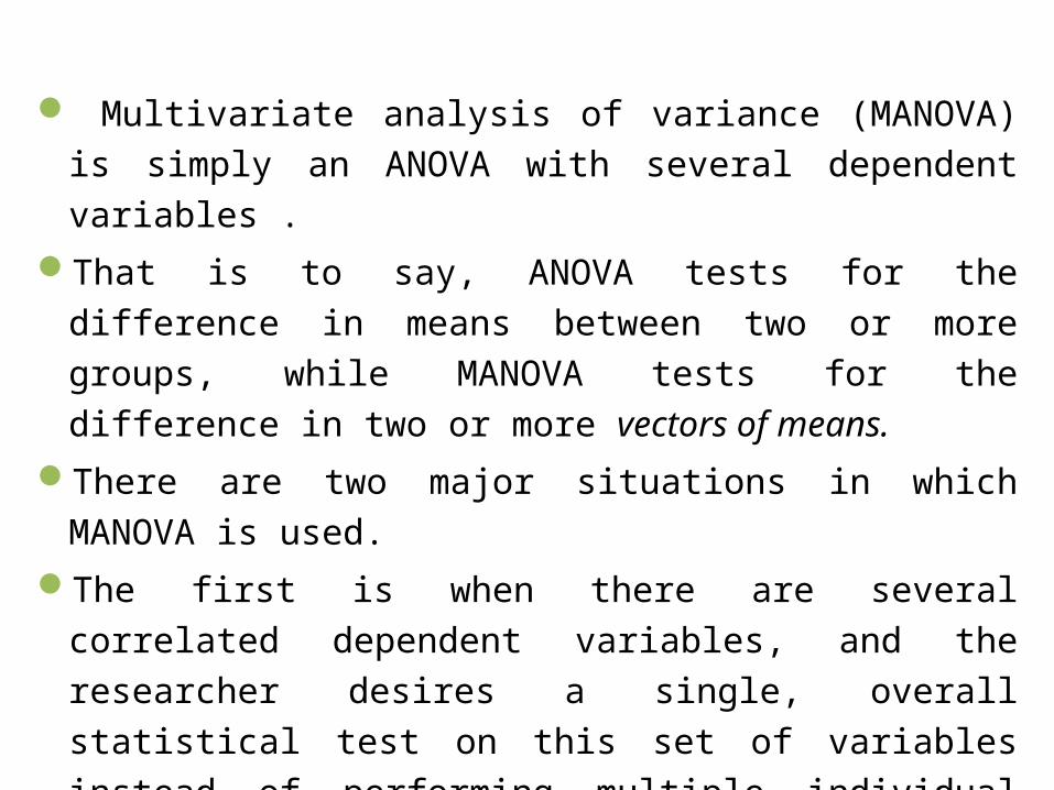
Multivariate analysis of variance (MANOVA) is simply an ANOVA with several dependent variables .

That is to say, ANOVA tests for the difference in means between two or more groups, while MANOVA tests for the difference in two or more vectors of means.

There are two major situations in which MANOVA is used. The first is when there are several correlated dependent variables,

and the researcher desires a single, overall statistical test on this set of variables instead of performing multiple individual tests.

The second, and in some cases, the more important purpose is to explore how independent variables influence some patterning of response on the dependent variables.

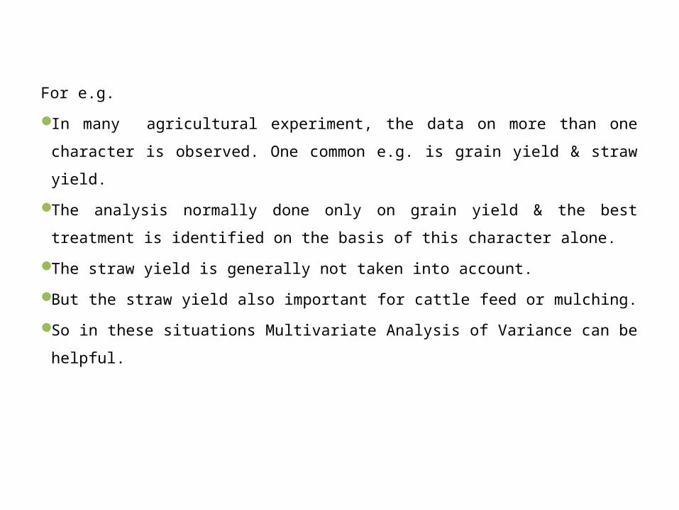
For e.g.

In many agricultural experiment, the data on more than one character

is observed. One common e.g. is grain yield & straw yield.

The analysis normally done only on grain yield & the best treatment is

identified on the basis of this character alone.

The straw yield is generally not taken into account.

But the straw yield also important for cattle feed or mulching.

So in these situations Multivariate Analysis of Variance can be helpful.

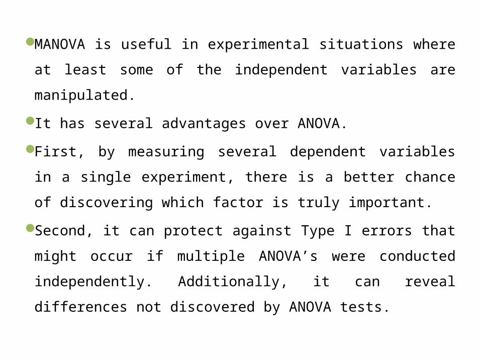
MANOVA is useful in experimental situations where at least

some of the independent variables are manipulated.

It has several advantages over ANOVA.

First, by measuring several dependent variables in a single

experiment, there is a better chance of discovering which factor

is truly important.

Second, it can protect against Type I errors that might occur if

multiple ANOVA’s were conducted independently. Additionally,

it can reveal differences not discovered by ANOVA tests.

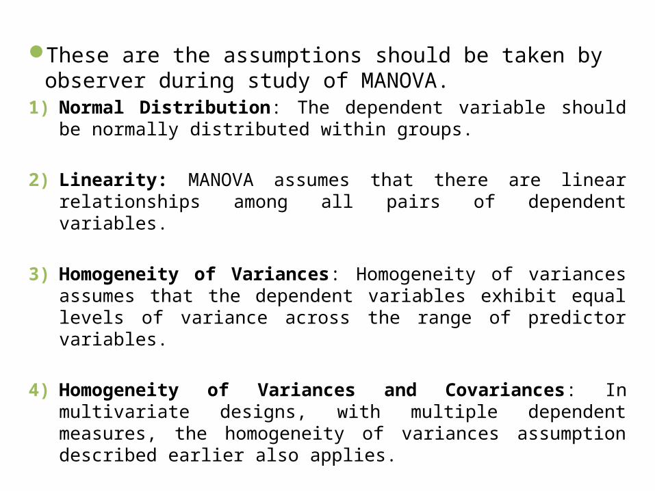
These are the assumptions should be taken by observer during study of MANOVA.

1) Normal Distribution: The dependent variable should be normally distributed within groups.

2) Linearity: MANOVA assumes that there are linear relationships among all pairs of dependent variables.

3) Homogeneity of Variances: Homogeneity of variances assumes that the dependent variables exhibit equal levels of variance across the range of predictor variables.

4) Homogeneity of Variances and Covariances: In multivariate designs, with multiple dependent measures, the homogeneity of variances assumption described earlier also applies.

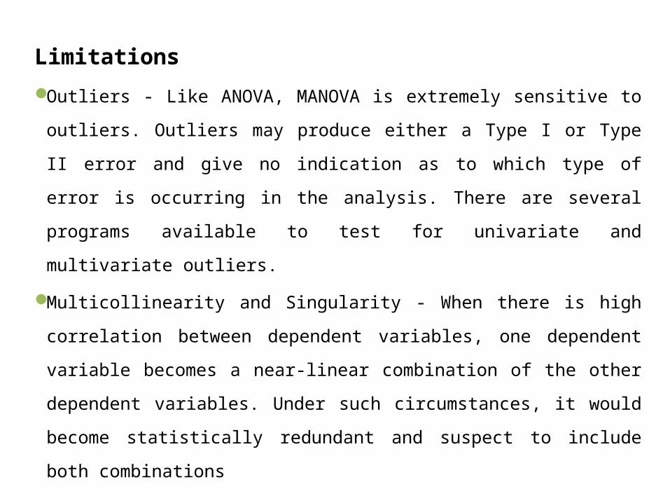
Limitations Outliers - Like ANOVA, MANOVA is extremely sensitive to outliers.

Outliers may produce either a Type I or Type II error and give no

indication as to which type of error is occurring in the analysis. There

are several programs available to test for univariate and multivariate

outliers.

Multicollinearity and Singularity - When there is high correlation

between dependent variables, one dependent variable becomes a

near-linear combination of the other dependent variables. Under such

circumstances, it would become statistically redundant and suspect to

include both combinations

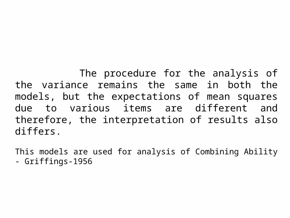
The procedure for the analysis of the variance remains the same in both the models, but the expectations of mean squares due to various items are different and therefore, the interpretation of results also differs.

This models are used for analysis of Combining Ability - Griffings-1956

Example 1. The yield of 6 varieties of a Wheat in kg./ plot are given in following table. The experiment was conducted using randomized block design with 5 replication.Treatment Replication Treatment

TotalTreatment

Mean

1 2 3 4 5

V1 20 26 30 28 23 127 25.40

V2 09 12 16 16 07 54 10.80

V3 12 15 14 14 14 71 14.20

V4 17 10 23 23 20 90 18.00

V5 28 26 35 35 30 140 28.40

V6 40 50 64 64 70 280 56.00

Total 126 139 180 180 164 764 25.46

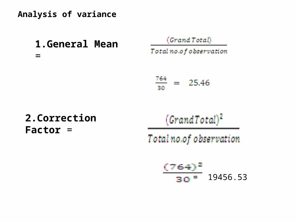
1.General Mean =

2.Correction Factor =

= 19456.53

Analysis of variance

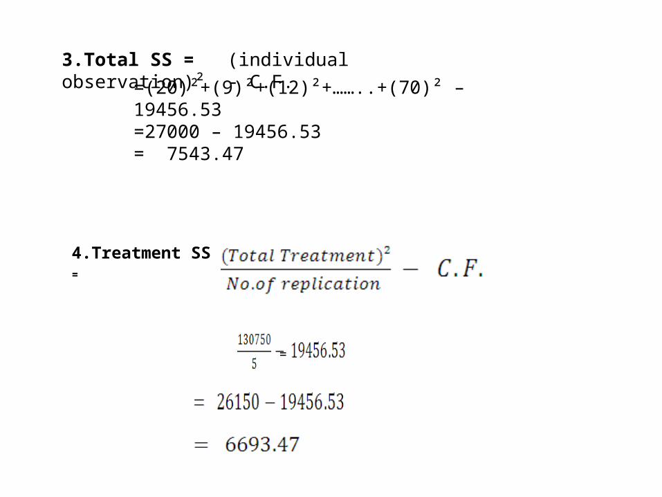
3.Total SS = (individual observation)² - C.F. =(20)²+(9)²+(12)²+……..+(70)² – 19456.53 =27000 – 19456.53 = 7543.47

4.Treatment SS =

=

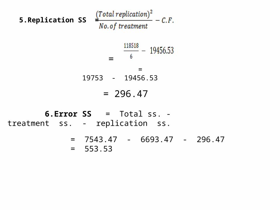
5.Replication SS =

=

= 19753 - 19456.53

= 296.47

6.Error SS = Total ss. - treatment ss. - replication ss.

= 7543.47 - 6693.47 - 296.47 = 553.53

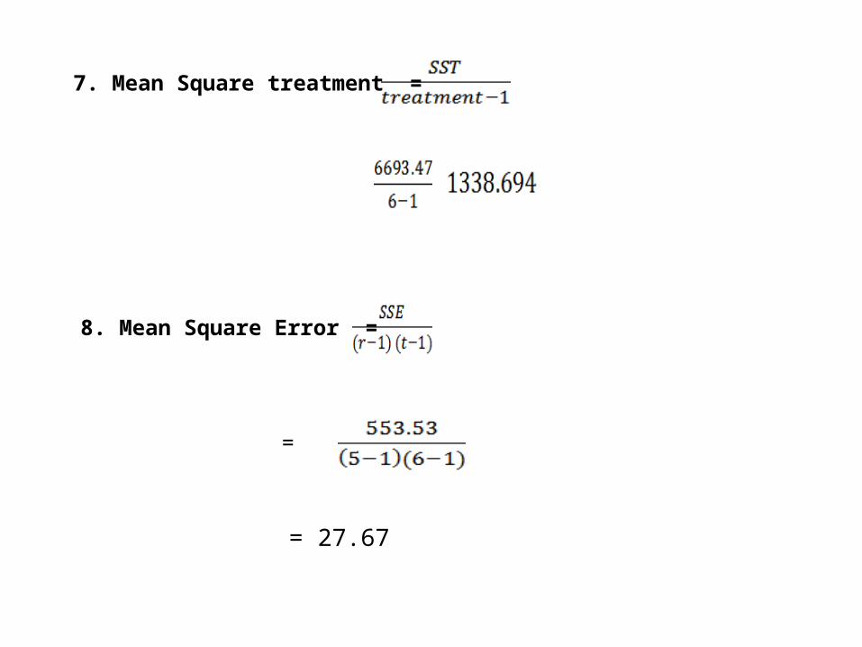
7. Mean Square treatment =

8. Mean Square Error =

=

= 27.67

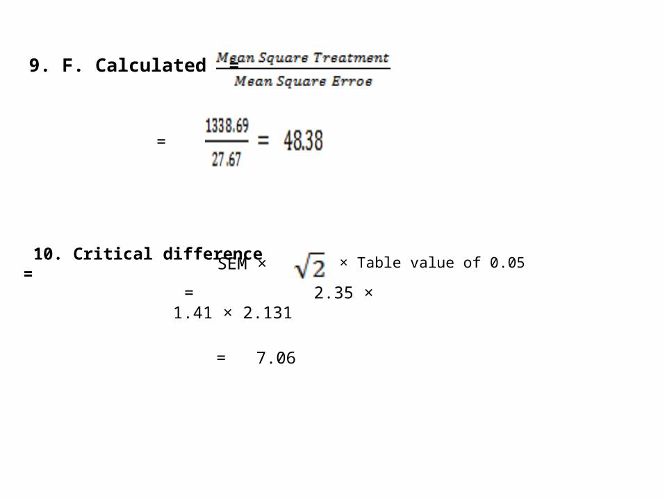
9. F. Calculated =

=

10. Critical difference = SEM × × Table value of 0.05

= 2.35 × 1.41 × 2.131

= 7.06

11. Standard error of mean =

12. Coefficient of variation =

= 20.66

(C V %)

Source of Variation

Degree of

Freedom

S. S. M. S. F. Calculation

F. Table Value

SEM C. D. C V%

Treatment 4 296.47 74.117 2.68

Replication 5 6693.47 1338.693 48.38

Error 20 553.53 27.67 2.137 2.35 7.06 20.66

Total 29 7543.47 1440.48

ANOVA Table

Advantages:

In this design more then one units can be used to one or some treatment in each replication.

In the statistical analysis, even when more then one units are used to a treatment per replication remains simpler.

Any no. of treatment can be tried in this design however this depends upon the homogeneity of the material within a group of the replication.

Disadvantage: If the grouping does not assure complete elimination of heterogeneity among experimental units requires further grouping and ultimately this design is less efficient.

If the observations are missing one has to estimate the missing observations and then analyses the data. If large no. of observations are missing one may be even able to analysis the data.

References

• Falconer DS & Mackay J. 1998. Introduction to Quantitative Genetics. Longman.• Mather K & Jinks JL. 1971. Biometrical Genetics. Chapman & Hall.• Naryanan SS & Singh P. 2007. Biometrical Techniques in Plant Breeding. Kalyani.

THANK YOU