LAB-BASED STATISTIC (PSYC 3100)

SEMESTER 1, 2014/2015

E-PORTFOLIO

SITI SUHAILA BINTI KHAIRIL-ANWAR

1212994

SECTION 2

LECTURER:

ASST. DR. HARRIS SHAH ABD HAMID

• The scales that I use for this e-portfolio is

Agreeableness Scale and Attitudes towards Woman

Scale.

• The Agreeableness Scale was taken from the Big

Five Personality Test while the Attitudes towards

Woman Scale was taken from the short version of

Spence, Helmrich & Stapp (1978) Attitudes towards

Woman Scale.

• Both of the scales have their own way to compute

the scores, which will be explained later.

• All of the data collected can be referred from the

folder under the name “Lab-Based questionnaire

ANSWERED BY PARTICIPANTS”.

1. DATA

ENTRY

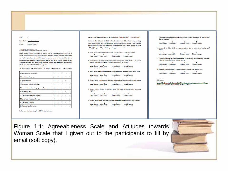
Figure 1.1: Agreeableness Scale and Attitudes towards

Woman Scale that I given out to the participants to fill by

email (soft copy).

Figure 1.2: Example of questionnaire that participant has

answered.

Figure 1.3: The variable view of SPSS. The variables named

according to their types and the items of both of the scales

name with ItemA and ItemB.

Figure 1.4: The data view of SPSS is where all the data

collected from the questionnaires; the scores, were entered.

Figure 1.5: The ItemB2, ItemB3, ItemB5 and ItemB6 of

Attitudes toward Womans are RECODE as they were a

Reverse Likert Scores.

Figure 1.6: The ItemB2, ItemB3, ItemB5 and ItemB6 of

Attitudes toward Womans are RECODED.

2.

TRANSFORM

Figure 2.1: The items of Agreeableness Scale computed

according to the Big Five Personality Test guidelines under

the name “Agreeableness”.

Figure 2.2: The items of Agreeableness Scale computed

according to the Big Five Personality Test guidelines under

the name “Agreeableness”.

3. RECODE

Figure 3.1: The Agreeableness scores recoded into

different variables named “AgreeablenessLevel” as the

scores were recoded into three ordinal level of

agreeablenes personality.

Figure 3.2: The Agreeableness scores recoded into three

level of agreeableness based on the range. 1-13 total score

recoded as 1, 14-26 total score recoded as 2 and more

than total scores of 27 recoded as 3.

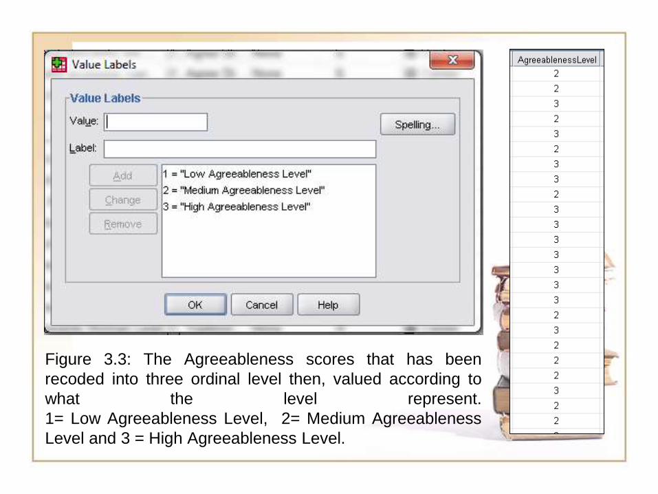
Figure 3.3: The Agreeableness scores that has been

recoded into three ordinal level then, valued according to

what the level represent.

1= Low Agreeableness Level, 2= Medium Agreeableness

Level and 3 = High Agreeableness Level.

Figure 3.4: The Attitudes Towards Woman scores recoded

into different variables named “ATWLevel” as the scores

were recoded into three level of attitudes.

Figure 3.5: The Attitudes Towards Woman scores also

recoded into three level of attitudes based on the range. 1-

13 total score recoded as 1, 14-26 total score recoded as 2

and more than total scores of 27 recoded as 3.

Figure 3.6: The Attitudes Towards Woman scores that has

been recoded into three level then, valued according to

what the level represent.

1= Traditional; Conservative Attitudes Towards Woman, 2=

Neutral Attitudes Towards Woman and 3 = Profeminist;

Egalitarian Attitudes Towards Woman.

4. NAMING OF

VARIABLE AND ITS

CHARACTERISTIC

S

Figure 4.1: This figure show the variable view of SPSS Data

Editor. All the variables were named according to what they

represented for.

• Figure 4.1 shows the demographic variables which are the

demographic background information of the participants (the first

five variables).

• The demographic variables are ID, Age, Month, Year and Gender.

• ID is the identifier of participants which define by using numbering.

• Age is the current age of the participants.

• Month and year is the birth month and year of the

participants.

• Gender is the sex of the participants either male or

female. The male participant represented as 1

while female represented by number 2.

• The demographic variables are ID, Age, and Year are considered

as nominal because of its nature and they have no value label.

• Month and Gender have value label as the month label by number

from 1 to 10 rather than write the name of each month and gender 1

for male and 2 for female.

• Next ten variables are the items or questions of

Agreeableness Scale which were named as ItemA.

• All of the items named according to their number of

question like question number one named as

ItemA1, question number two named as ItemA2

and so on until question number 10; ItemA10.

• All ItemA have value labels; 1= I disagree a lot, 2= I disagree a

little, 3= Neutral, 4= I agree a little and 5 = I agree a lot.

• Last ten variables in the Figure 4.1 are the questions of Attitudes

towards Woman Scale which were named as ItemB plus with

number of each question like question one ItemB1.

• All ten item were name ItemB1, ItemB2, ItemB3,

ItemB4, ItemB5, ItemB6, ItemB7, ItemB8, ItemB9,

and ItemB10 and they were valued with :

1= Agree strongly, 2= Agree mildly,

3= Disagree mildly and 4= Disagree strongly .

Figure 4.2: This figure shows the computed variable from all ItemA of

Agreeableness Scale; Agreeableness and computed variable of all

ItemB of Attitude Towards Woman Scale; ATW.

• Agreeableness is total scores of all ItemA which

can get from compute the data.

• ATW is stand for ‘Atitudes towards Woman’ and

also a total scores of all ItemB which get by

computing the data.

• AgreeablenesLevel variable is a recoded data of

Agreeableness. The score have been valued as;

1= Low Agreeableness, 2= Medium

Agreeableness, and 3= High Agreeableness.

• ATWLevel is a recoded variable from ATW total scores. The value

lable of this variable is 1= Traditional;

Conservative, 2= Neutral and 3= Profeminist; Egalitarian.

• All of the ItemA and ItemB are categorized as Scale as they are

considered under interval measurement.

• Same goes for the Agreeableness, ATW, AgreeablenessLevel, and

ATWLevel.

5. DATA

SCREENING

Figure 5.1: Errors or missing value can be check through the

frequency table, minimum and maximum values.

Figure 5.2: Put all the possible variables to check any error or

missing values and execute the command.

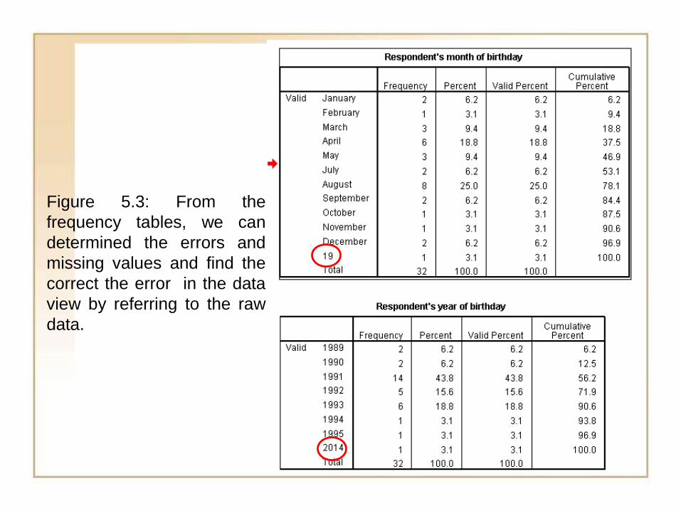
Figure 5.3: From the

frequency tables, we can

determined the errors and

missing values and find the

correct the error in the data

view by referring to the raw

data.

Figure 5.4: From the frequency tables, we can determined

the errors and missing values and find the correct the

error in the data view by referring to the raw data.

Figure 5.5: From the

frequency tables, we can

determined the errors and

missing values and find the

correct the error in the data

view by referring to the raw

data.

Figure 5.6: The data view of SPSS is where all the data

collected from the questionnaires; the scores, were entered.

The highlighted boxes are the errors and missing value that

we determined from the frequency tables.

• After screening and corrected the data, the frequency table will be

cleaned without any errors and missing values.

• The corrected errors are:

1) Valid value of 19 in the month of birthday of participant with

ID number 7 is actually 9 which represent month of

September.

2) Valid value of 2014 in the year of birthday of participant with

ID number 32 is actually 1993.

3) The value of missing value for participant

with ID 5 in ItemA3 is 3. The participant

made two answer for the previous question

which is ItemA2.

4) The same mistakes happened to participant

with ID number 13 and 17 were mistakenly

gave two answer on the previous item of

ItemB7 and the later question of ItemB1.

Figure 5.7: From the

frequency tables, we can

see now, the frequency

table is cleaned from any

errors and missing values.

Figure 5.8: From the statistic tables, we can see now, the frequency table

is cleaned from any errors and missing values.

Figure 5.9: From the Agreeableness frequency table, we

can see now, the frequency table is cleaned from any

errors and missing values.

Figure 5.10: From the Attitudes Towards Woman

frequency table, we can see now, the frequency table is

cleaned from any errors and missing values.

6. NORMAL

DISTRIBUTION

OF DATA

Figure 6.1: Figure shows the steps to use histogram to

check the normality of distribution.

After the data corrected, the next step is to check for the normality of

distribution. There are many ways to check the normality of data. There are

Histogram graph with normality curve, P-P and Q-Q plot, also the normality

statistic.

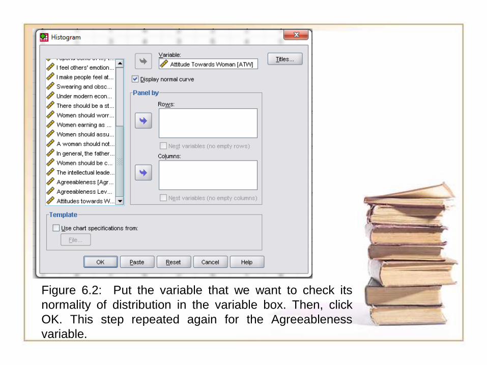
Figure 6.2: Put the variable that we want to check its

normality of distribution in the variable box. Then, click

OK. This step repeated again for the Agreeableness

variable.

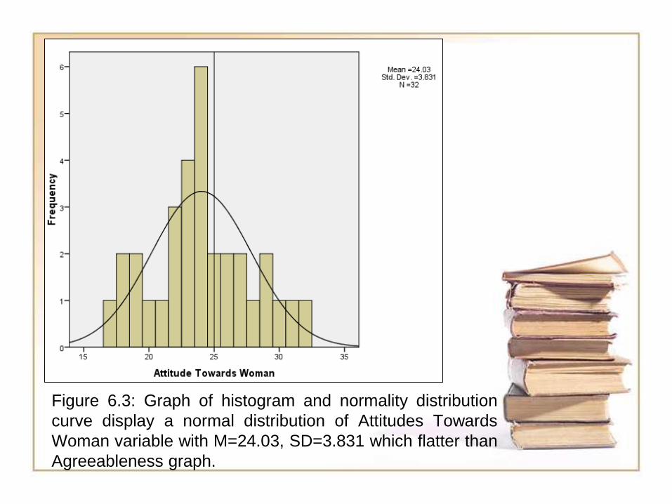
Figure 6.3: Graph of histogram and normality distribution

curve display a normal distribution of Attitudes Towards

Woman variable with M=24.03, SD=3.831 which flatter than

Agreeableness graph.

Figure 6.4: Graph of histogram and normality distribution curve

display a normal distribution of Agreeableness variable with

M=24.03, SD=3.831. The distribution of Agreeableness are more

sharper than the ATW Graph.

Figure 6.5: The first P-P Plot graph of Attitudes Towards Woman

shows the dots are closely aligned to the straight line which prove

that the data is normally distributed compared to the second plot

graph Detrended Normal P-P plot of Attitudes Towards Woman is

more scattered.

Figure 6.6: The first Q-Q Plot of Attitudes Towards Woman, graph

shows the dots are closely aligned to the straight line which prove

that the data is normally distributed compared to the second plot

graph which is more scattered.

Figure 6.7: The first P-P plot graph of Agreeableness shows the

dots are closely aligned to the straight line which prove that the

data is normally distributed compared to the second plot graph

which is more scattered.

Figure 6.8: The first Q-Q plot graph of Agreeableness shows that

the dots are closely aligned to the straight line which prove that the

data is normally distributed while the second plot graph which is

Detrended Normal Q-Q plot is more fluctuated.

Figure 6.9: Normality Statistic is the numerical method to check normality of

distribution. Skewness and Kurtosis values that are significantly from zero may

indicate non-normality of distribution. To calculate the acceptable value, take the

statistic and divide with its standard error. For example, the Skewness index for

Agreeableness is 0.465/0.414= 1.123. Index values within +/-1.96 indicate normality

of distribution.

• From the Figure 6.9, the Agreeableness variable is normally

distributed as its index value is 1.123 which within the +/-1.96 .

• For variable of Attitudes towards Woman, the index is

0.165/0.414= 0.399 which lies within the +/-1.96 boundary that

indicate normality of distribution.

7.

PRESENTATIO

N

• Evidence of transfer of output from SPSS to MS Word can

be referred to document named “7.Presentation”.