Embed Size (px)
Citation preview
Yue Wu, Biaobiao Zhang, Jiabin Lu & K. -L. Du
International Journal of Artificial Intelligence and Expert Systems (IJAE), Volume (2) : Issue (2) : 2011 47
Fuzzy Logic and Neuro-fuzzy Systems: A Systematic
Introduction
Yue Wu [email protected]
Enjoyor Inc
Hangzhou, 310030, China
Biaobiao Zhang [email protected]
Enjoyor Inc
Hangzhou, 310030, China
Jiabin Lu [email protected]
Faculty of Electromechanical Engineering
Guangdong University of Technology
Guangzhou, 510006, China
K. -L. Du [email protected]
Department of Electrical and Computer Engineering
Concordia University
Montreal, H3G 1M8, Canada
and
Enjoyor Inc
Hangzhou, 310030, China
Abstract
Fuzzy logic is a rigorous mathematical field, and it provides an effective vehicle for modeling the
uncertainty in human reasoning. In fuzzy logic, the knowledge of experts is modeled by linguistic
rules represented in the form of IF-THEN logic. Like neural network models such as the multilayer
perceptron (MLP) and the radial basis function network (RBFN), some fuzzy inference systems
(FISs) have the capability of universal approximation. Fuzzy logic can be used in most areas
where neural networks are applicable. In this paper, we first give an introduction to fuzzy sets and
logic. We then make a comparison between FISs and some neural network models. Rule
extraction from trained neural networks or numerical data is then described. We finally introduce
the synergy of neural and fuzzy systems, and describe some neuro-fuzzy models as well. Some
circuits implementations of neuro-fuzzy systems are also introduced. Examples are given to
illustrate the concepts of neuro-fuzzy systems.
Keywords: Fuzzy Set, Fuzzy Logic, Fuzzy Inference System, Neuro-fuzzy System, Neural
Network, Mamdani Model, Takagi-Sugeno-Kang Model.
1. INTRODUCTION
Fuzzy set, a concept first proposed by Zadeh [123], is a method for modeling the uncertainty in
human reasoning. Fuzzy logic is suitable for the representation of vague data and concepts on
an intuitive basis, such as human linguistic description, e.g. the expressions approximately, large,
young. The conventional set, also called the crisp set, can be treated as a special form of fuzzy
set. Unlike the binary logic, fuzzy logic uses the notion of membership. A fuzzy set is uniquely
determined by its membership function (MF), and it is also associated with a linguistically
meaningful term.
Yue Wu, Biaobiao Zhang, Jiabin Lu & K. -L. Du
International Journal of Artificial Intelligence and Expert Systems (IJAE), Volume (2) : Issue (2) : 2011 48
Fuzzy logic provides a systematic tool to incorporate human experience. It is based on three core
concepts, namely, fuzzy sets, linguistic variables, and possibility distributions. Fuzzy set is used
to characterize linguistic variables whose values can be described qualitatively using a linguistic
expression and quantitatively using an MF [124]. Linguistic expressions are useful for
communicating concepts and knowledge with human beings, whereas MFs are useful for
processing numeric input data. When a fuzzy set is assigned to a linguistic variable, it imposes an
elastic constraint, called a possibility distribution, on the possible values of the variable.
Fuzzy logic is a rigorous mathematical discipline. Fuzzy reasoning is a straightforward formalism
for encoding human knowledge or common sense in a numerical framework, and FISs can
approximate arbitrarily well any continuous function on a compact domain [55], [113]. FISs and
feedforward neural networks (FNNs) can approximate each other to any degree of accuracy [13].
Fuzzy logic first found popular applications in control systems, where an FIS is built up by
codifying human knowledge as linguistic IF-THEN rules. Since its first reported industrial
application in 1982 [41], it has aroused global interest in the industrial and scientific community,
and fuzzy logic has also been widely applied in data analysis, regression and prediction, as well
as signal and image processing. Many application-specific integrated circuits (ASICs) has also
been designed for fuzzy logic [31].
In this paper, we give a systematic introduction to fuzzy logic and neuro-fuzzy systems. The
paper is organized as follows. In Section 2, we provide a short tutorial on fuzzy logic. Section 3
compares fuzzy logic and neural network paradigms. Section 4 compares the relation between
fuzzy logic and MLP/RBFN, and rule generation from trained neural networks is introduced in this
section. Rule extraction from numerical data is introduced in Section 5. The paradigm of neuro-
fuzzy systems is described in Section 6. Some neuro-fuzzy models are introduced in Section 7. In
Section 8, we describe some fuzzy neural circuits. An illustration of using neuro-fuzzy systems is
given in Section 9. We summarize this paper in Section 10.
2. FUNDAMENTALS OF FUZZY LOGIC
2.1 Definitions
We list below some definitions and terminologies used in the fuzzy logic literature.
2.1.1 Universe of Discourse
The universal set 𝑋: 𝑋 → [0,1] is called the universe of discourse, or simply the universe. The
implication 𝑋 → [0,1] is the abbreviation for the IF-THEN rule: ―IF 𝑥 is in 𝑋, THEN its MF 𝜇𝑋(𝑥) is
in [0,1].‖, where 𝜇𝑋(𝑥) is the MF of 𝑥. The universe 𝑋 may contain either discrete or continuous
values.
2.1.2 Linguistic Variable
A linguistic variable is a variable whose values are linguistic terms in a natural or artificial
language. For example, the size of an object is a linguistic variable, whose value can be small,
medium, and big.
2.1.3 Fuzzy Set
A fuzzy set 𝐴 in 𝑋 is defined by
𝐴 = 𝑥, 𝜇𝐴 𝑥 𝑥 ∈ 𝑋 , (1)
where 𝜇𝐴 𝑥 ∈ [0,1] is the MF of 𝑥 in 𝐴. For 𝜇𝐴 𝑥 , the value 1 stands for complete membership
of the set 𝐴, while 0 represents that 𝑥 does not belong to the set at all. A fuzzy set can also be
syntactically represented by
Yue Wu, Biaobiao Zhang, Jiabin Lu & K. -L. Du
International Journal of Artificial Intelligence and Expert Systems (IJAE), Volume (2) : Issue (2) : 2011 49
𝐴 =
𝜇𝐴(𝑥𝑖)
𝑥𝑖𝑥𝑖∈𝑋
, if 𝑋 is discrete
𝜇𝐴(𝑥)
𝑥𝑋
, if 𝑋 is continuous
. (2)
2.1.4 Support
The elements on fuzzy set 𝐴 whose membership is larger than zero are called the support of 𝐴
sp 𝐴 = 𝑥 ∈ 𝐴 𝜇𝐴 𝑥 > 0 . (3)
2.1.5 Height
The height of a fuzzy set 𝐴 is defined by
hgt 𝐴 = sup 𝜇𝐴 𝑥 𝑥 ∈ 𝑋 . (4)
2.1.6 Normal Fuzzy Set and Non-normal Fuzzy Set
A fuzzy set 𝐴 is said to be normal if hgt(𝐴) = 1. If 0 < hgt(𝐴) < 1, the fuzzy set 𝐴 is said to be
non-normal. The non-normal fuzzy set can be normalized by dividing the height of 𝐴 , i.e.,
𝜇 𝐴(𝑥) = 𝜇𝐴 (𝑥)
hgt (𝐴).
2.1.7 Fuzzy Subset
A fuzzy set 𝐴 = 𝑥, 𝜇𝐴 𝑥 𝑥 ∈ 𝑋 is said to be a fuzzy subset of 𝐵 = 𝑥, 𝜇𝐵 𝑥 𝑥 ∈ 𝑋 if
𝜇𝐴 𝑥 ≤ 𝜇𝐵 𝑥 , denoted by 𝐴 ⊆ 𝐵.
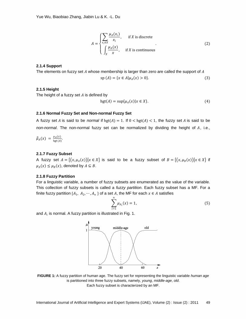
2.1.8 Fuzzy Partition
For a linguistic variable, a number of fuzzy subsets are enumerated as the value of the variable.
This collection of fuzzy subsets is called a fuzzy partition. Each fuzzy subset has a MF. For a
finite fuzzy partition {𝐴1, 𝐴2, ⋯ , 𝐴𝑛 } of a set 𝐴, the MF for each 𝑥 ∈ 𝐴 satisfies
𝜇𝐴𝑖 𝑥 = 1
𝑛
𝑖=1
, (5)
and 𝐴𝑖 is normal. A fuzzy partition is illustrated in Fig. 1.
FIGURE 1: A fuzzy partition of human age. The fuzzy set for representing the linguistic variable human age
is partitioned into three fuzzy subsets, namely, young, middle-age, old.
Each fuzzy subset is characterized by an MF.
Yue Wu, Biaobiao Zhang, Jiabin Lu & K. -L. Du
International Journal of Artificial Intelligence and Expert Systems (IJAE), Volume (2) : Issue (2) : 2011 50
2.1.9 Empty Set
The subset of 𝑋 having no element is called the empty set, denoted by ∅ .
2.1.10 Complement
The complement of 𝐴, written 𝐴 , ¬𝐴 or NOT 𝐴, is defined as 𝜇𝐴 (𝑥) = 1 − 𝜇𝐴(𝑥). Thus, 𝑋 = ∅ and
∅ = 𝑋.
2.1.11 𝜶-cut
The 𝛼-cut or 𝛼-level set of a fuzzy set 𝐴, written 𝜇𝐴[𝛼], is defined as
𝜇𝐴 𝛼 = 𝑥 ∈ 𝐴 𝜇𝐴 𝑥 ≥ 𝛼 , (6)
where 𝛼 ∈ [0,1]. For continuous sets, 𝜇𝐴 [𝛼] can be characterized by an interval or a union of
intervals.
2.1.12 Kernel or Core
All the elements in a fuzzy set 𝐴 with membership degree 1 constitute a subset called the kernel
or core of the fuzzy set, written as co(𝐴) = 𝜇𝐴 [1].
2.1.13 Convex Fuzzy Set
A fuzzy set 𝐴 is said to be convex if and only if
𝜇𝐴 𝜆𝑥1 + 1 − 𝜆 𝑥2 ≥ 𝜇𝐴 𝑥1 ∧ 𝜇𝐴 𝑥2 (7)
for 𝜆 ∈ [0,1], and 𝑥1, 𝑥2 ∈ 𝑋, where ∧ denotes the minimum operation. Any 𝛼-cut set of a convex
fuzzy set is a closed interval.
2.1.14 Concave Fuzzy Set
A fuzzy set 𝐴 is said to be concave if and only if
𝜇𝐴 𝜆𝑥1 + 1 − 𝜆 𝑥2 ≤ 𝜇𝐴 𝑥1 ∨ 𝜇𝐴 𝑥2 . (8)
For 𝜆 ∈ [0,1], and 𝑥1, 𝑥2 ∈ 𝑋, where ∨ denotes the maximum operation.
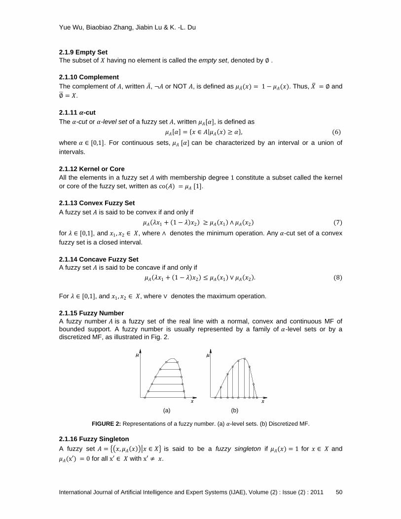
2.1.15 Fuzzy Number
A fuzzy number 𝐴 is a fuzzy set of the real line with a normal, convex and continuous MF of
bounded support. A fuzzy number is usually represented by a family of 𝛼-level sets or by a
discretized MF, as illustrated in Fig. 2.
(a) (b)
FIGURE 2: Representations of a fuzzy number. (a) 𝛼-level sets. (b) Discretized MF.
2.1.16 Fuzzy Singleton
A fuzzy set 𝐴 = 𝑥, 𝜇𝐴 𝑥 𝑥 ∈ 𝑋 is said to be a fuzzy singleton if 𝜇𝐴(𝑥) = 1 for 𝑥 ∈ 𝑋 and
𝜇𝐴(x′) = 0 for all x′ ∈ 𝑋 with x′ ≠ 𝑥.
Yue Wu, Biaobiao Zhang, Jiabin Lu & K. -L. Du
International Journal of Artificial Intelligence and Expert Systems (IJAE), Volume (2) : Issue (2) : 2011 51
2.1.17 Hedge
A hedge transforms a fuzzy set into a new fuzzy set. A hedge operator is comparable to an
adverb in English. Hedges are used to intensify or dilute the characteristic of a fuzzy set such as
very and quite, or to approximate a fuzzy set or convert a scalar to a fuzzy set such as roughly.
For example, for a fuzzy set strong with membership degree 𝜇𝐴 𝑥 , very strong can be described
using the membership degree 𝜇𝐴2 𝑥 , while quite strong can be described using the membership
degree 𝜇𝐴
1
2 𝑥 .
2.1.18 Extension Principle
Given mapping 𝑓: 𝑋 → 𝑌 and a fuzzy set 𝐴 = 𝑥, 𝜇𝐴 𝑥 𝑥 ∈ 𝑋 , the extension principle is given
by
𝑓(𝐴) = 𝑓 𝑥 , 𝜇𝐴 𝑥 𝑥 ∈ 𝑋 . (9)
2.1.19 Cartesian Product
If 𝑋 and 𝑌 are two universal sets, then 𝑋 × 𝑌 is the set of all ordered pairs (𝑥, 𝑦) for 𝑥 ∈ 𝑋 and
𝑦 ∈ 𝑌. Let 𝐴 be a fuzzy set of 𝑋 and 𝐵 a fuzzy set of 𝑌. The Cartesian product is defined as
𝐴 × 𝐵 = 𝑧, 𝜇𝐴×𝐵 𝑧 𝑧 = 𝑥, 𝑦 ∈ 𝑍, 𝑍 = 𝑋 × 𝑌 , (10)
where 𝜇𝐴×𝐵 𝑧 = 𝜇𝐴 𝑥 ∧ 𝜇𝐵 𝑥 , ∧ denoting the 𝑡-norm operation.
2.1.20 Fuzzy Relation
Fuzzy relation is used to describe the association between two things. If 𝑅 is a subset of 𝑋 × 𝑌,
then 𝑅 is said to be a relation between 𝑋 and 𝑌, or a relation on 𝑋 × 𝑌. Mathematically,
𝑅 𝑥, 𝑦 = 𝑥, 𝑦 , 𝜇𝑅 𝑥, 𝑦 𝑥, 𝑦 ∈ 𝑋 × 𝑌, 𝜇𝑅 𝑥, 𝑦 ∈ [0,1] , (11)
where 𝜇𝑅 𝑥, 𝑦 is the degree of membership for association between 𝑥 and 𝑦. A fuzzy relation is
also a fuzzy set.
2.1.21 Fuzzy Matrix and Fuzzy Graph
Given finite, discrete fuzzy sets 𝑋 = { 𝑥1, 𝑥2 , ⋯ , 𝑥𝑚 } and Y = {𝑦1, … , 𝑦𝑛}, a fuzzy relation on 𝑋 × 𝑌
can be represented by an 𝑚 × 𝑛 matrix 𝐑 = [ 𝑅𝑖𝑗 ] = [ 𝜇𝑅 ( 𝑥𝑖 , 𝑦𝑗 )]. This matrix is called a fuzzy
matrix. The fuzzy relation 𝑅 can be represented by a fuzzy graph. In a fuzzy graph, all 𝑥𝑖 and 𝑦𝑗
are vertices, and the grade 𝜇𝑅(𝑥𝑖 , 𝑦𝑗 ) is added to the connection from 𝑥𝑖 and 𝑦𝑗 .
2.1.22 𝒕-norm
A mapping 𝑇: 0,1 × 0,1 → [0,1] with the following four properties is called 𝑡 -norm. For all
𝑥, 𝑦, 𝑧 ∈ [0,1],
Commutativity: 𝑇(𝑥, 𝑦) = 𝑇(𝑦, 𝑥);
Monotonicity: 𝑇 𝑥, 𝑦 ≤ 𝑇 𝑥, 𝑧 , if 𝑦 ≤ 𝑧;
Associativity: 𝑇(𝑥, 𝑇(𝑦, 𝑧)) = 𝑇(𝑇(𝑥, 𝑦), 𝑧);
Linearity: 𝑇(𝑥, 1) = 𝑥.
2.1.23 𝒕-conorm
A mapping C: 0,1 × 0,1 → [0,1] having the following four properties is called 𝑡-conorm. For all
𝑥, 𝑦, 𝑧 ∈ [0,1],
Commutativity: 𝐶(𝑥, 𝑦) = 𝐶(𝑦, 𝑥);
Monotonicity: 𝐶 𝑥, 𝑦 ≤ 𝐶(𝑥, 𝑧), if 𝑦 ≤ 𝑧;
Yue Wu, Biaobiao Zhang, Jiabin Lu & K. -L. Du
International Journal of Artificial Intelligence and Expert Systems (IJAE), Volume (2) : Issue (2) : 2011 52
Associativity: 𝐶(𝑥, 𝐶(𝑦, 𝑧)) = 𝐶(𝐶(𝑥, 𝑦), 𝑧);
Linearity: 𝐶(𝑥, 0) = 𝑥.
2.2 Membership Function
A fuzzy set 𝐴 over the universe of discourse 𝑋, 𝐴 ⊆ 𝑋 → [0,1], is described by the degree of
membership 𝜇𝐴 𝑥 ∈ [0,1] for each 𝑥 ∈ 𝑋. Unimodality and normality are two important aspects of
the MFs [23]. Piecewise-linear functions such as triangles and trapezoids are popular MFs. The
triangular MFs can be defined by
𝜇 𝑥; 𝑎, 𝑏, 𝑐 =
𝑥 − 𝑎
𝑏 − 𝑎, 𝑎 ≤ 𝑥 ≤ 𝑏
𝑐 − 𝑥
𝑐 − 𝑏, 𝑏 < 𝑥 ≤ 𝑐
0, otherwise
, (12)
where the shape parameters satisfies 𝑎 ≤ 𝑏 ≤ 𝑐 , and 𝑏 ∈ 𝑋 . Triangular MFs are useful for
modeling fuzzy numbers or linguistic terms such as ―The temperature is about 20∘ C‖. The
trapezoid MFs have flat top with constant value 1. Trapezoid MFs are suitable for modeling such
linguistic terms as ―He looks like a teenager‖.
The Gaussian and bell-shaped functions have continuous derivatives, and are usually used to
replace the triangular MF when shape parameters are adapted using the gradient-descent
procedure. Another popular MF is a sigmoidal functions of the form
𝜇 𝑥; 𝑐, 𝛽 =1
1 + e−𝛽(𝑥−𝑐), (13)
where 𝑐 shifts the function to the left or to the right, and 𝛽 controls the shape of the function.
When 𝛽 > 1 it is an S-shaped function, and when 𝛽 < −1 it is a Z-shaped function. By multiplying
an S-shaped function by a Z-shaped function, a 𝜋-shaped function is obtained [29]. 𝜋-shaped
MFs can be used in situations similar to that where trapezoid MFs are used.
2.3 Intersection and Union
The set operations intersection and union correspond to the logic operations conjunction (AND)
and disjunction (OR), respectively. Intersection is described by the so-called triangular norm (𝑡-
norm), denoted by 𝑇(𝑥, 𝑦), whereas union is described by the so-called triangular conorm (𝑡-
conorm), denoted by 𝐶(𝑥, 𝑦).
If 𝐴 and 𝐵 are fuzzy subsets of 𝑋, then intersection 𝐼 = 𝐴 ∩ 𝐵 is defined by
𝜇𝐼 𝑥 = 𝑇 𝜇𝐴 𝑥 , 𝜇𝐵 𝑥 . (14)
Basic 𝑡-norms are given as the standard intersection, the bound sum, the algebraic product and
the drastic intersection [14]. The popular standard intersection and algebraic product are
respectively defined by
𝑇m 𝑥, 𝑦 = min 𝑥, 𝑦 , (15)
𝑇p 𝑥, 𝑦 = 𝑥𝑦. (16)
Similarly, union 𝑈 = 𝐴 ∪ 𝐵 is defined by
𝜇𝑈(𝑥) = 𝐶 𝜇𝐴 𝑥 , 𝜇𝐵 𝑥 . (17)
Yue Wu, Biaobiao Zhang, Jiabin Lu & K. -L. Du
International Journal of Artificial Intelligence and Expert Systems (IJAE), Volume (2) : Issue (2) : 2011 53
The corresponding basic 𝑡-conorms are given as the standard union, the bounded sum, the
algebraic sum, and the drastic union [14]. Corresponding to the standard intersection and
algebraic product, the two popular 𝑡 -conorms are respectively the standard union and the
algebraic sum
𝐶m 𝑥, 𝑦 = max 𝑥, 𝑦 , (18)
𝐶p 𝑥, 𝑦 = 𝑥 + 𝑦 − 𝑥𝑦. (19)
When the 𝑡-norm and the 𝑡-conorm satisfy 1 − 𝑇(𝑥, 𝑦) = 𝐶(1 − 𝑥, 1 − 𝑦), they are said to be dual.
This makes De Morgan's laws A ∩ B = A ∪ B and A ∪ B = A ∩ B to still hold in fuzzy set theory.
The above 𝑡-norms and 𝑡-conorms with the same subscripts are dual. To satisfy the principle of
duality, they are usually used in pairs.
2.4 Aggregation, Fuzzy Implication, and Fuzzy Reasoning
Aggregation or composition operations on fuzzy sets provide a means for combining several sets
in order to produce a single fuzzy set. 𝑇-conorms are usually used as aggregation operators.
Consider the relations
𝑅1 𝑥, 𝑦 = 𝑥, 𝑦 , 𝜇𝑅1 𝑥, 𝑦 𝑥, 𝑦 ∈ 𝑋 × 𝑌, 𝜇𝑅1
𝑥, 𝑦 ∈ 0,1 , (20)
𝑅2 𝑦, 𝑧 = 𝑦, 𝑧 , 𝜇𝑅2 𝑦, 𝑧 𝑦, 𝑧 ∈ 𝑌 × 𝑍, 𝜇𝑅2
𝑦, 𝑧 ∈ 0,1 . (21)
The max-min composition, denoted by 𝑅1 ∘ 𝑅2 with MF 𝜇𝑅1∘ 𝑅2, is defined by
𝑅1 ∘ 𝑅2 = 𝑥, 𝑧 , max𝑦
min 𝜇𝑅1 𝑥, 𝑦 , 𝜇𝑅2
𝑦, 𝑧 𝑥, 𝑧 ∈ 𝑋 × 𝑍, 𝑦 ∈ 𝑌 . (22)
There are some other composition operations, such as the min-max composition, denoted by
𝑅1 ⋄ 𝑅2 with the difference that the role of max and min are interchanged. The two compositions
are related by 𝑅1 ⋄ 𝑅2 = 𝑅1
∘ 𝑅2 .
Fuzzy implication is used to represent fuzzy rules. It is a mapping 𝑓: 𝐴 → 𝐵 according to the fuzzy
relation 𝑅 on 𝐴 × 𝐵
𝑦, 𝜇𝐵 𝑦 = 𝑓 𝑥, 𝜇𝐴 𝑥 . (23)
Denote 𝑝 as ―𝑥 is 𝐴‖ and 𝑞 as ―𝑦 is 𝐵‖, then (23) can be stated as 𝑝 → 𝑞 (if 𝑝 then 𝑞). For a fuzzy
rule expressed as a fuzzy implication using the defined fuzzy relation 𝑅, the output linguistic
variable 𝐵 is denoted by 𝐵 = 𝐴 ∘ 𝑅, which is characterized by 𝜇𝐵 𝑦 =∨𝑥 ( 𝜇𝐴 𝑥 ∧ 𝜇𝑅(𝑥, 𝑦)).
Fuzzy reasoning, also called approximate reasoning, is an inference procedure for deriving
conclusions from a set of fuzzy rules and one or more conditions [51]. The compositional rule of
inference is the essential rational behind fuzzy reasoning. A simple example of fuzzy reasoning is
described here. Consider the fuzzy set 𝐴 = 𝑥, 𝜇𝐴 𝑥 𝑥 ∈ 𝑋 } and the fuzzy relation 𝑅 on 𝐴 × 𝐵,
given by 𝑅 𝑥, 𝑦 = 𝑥, 𝑦 , 𝜇𝑅 𝑥, 𝑦 𝑥, 𝑦 ∈ 𝑋 × 𝑌} . Fuzzy set 𝐵 can be inferred from fuzzy set
𝐴 and their fuzzy relation 𝑅 𝑥, 𝑦 by the max-min composition
𝐵 = 𝐴 ∘ 𝑅 = 𝑦, max𝑥
min 𝜇𝐴 𝑥 , 𝜇𝑅 𝑥, 𝑦 𝑥 ∈ 𝑋, 𝑦 ∈ 𝑌 . (24)
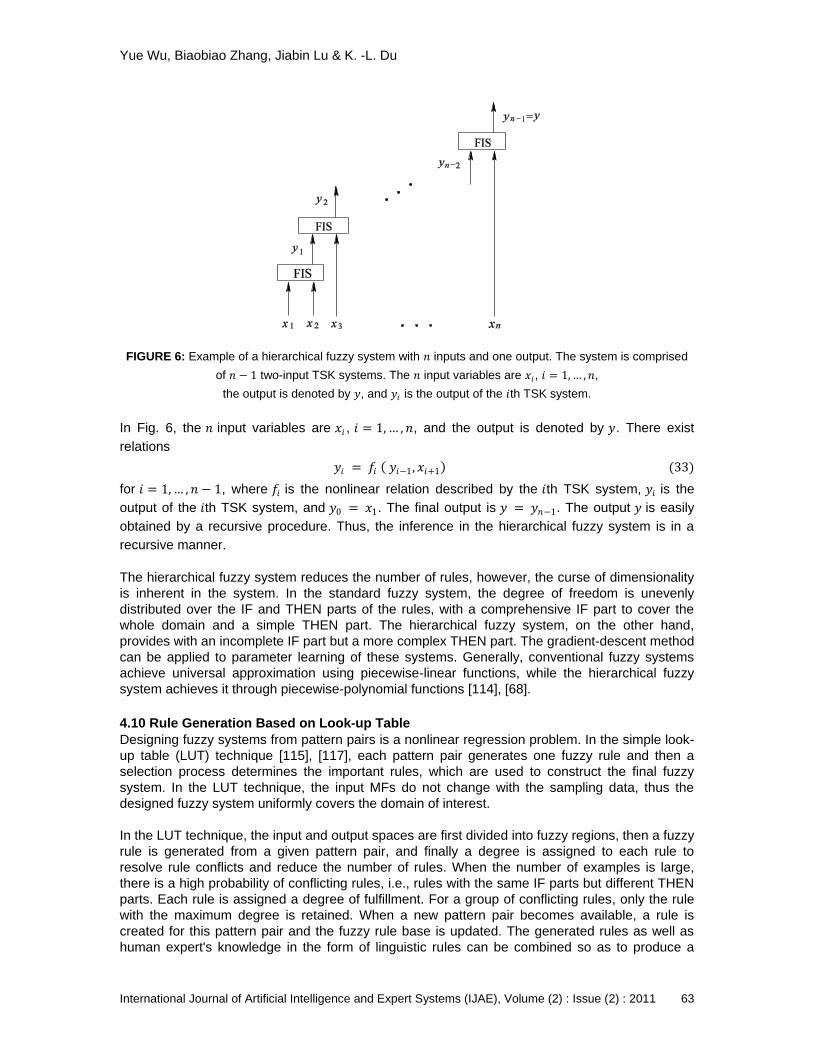
2.5 Fuzzy Inference Systems
In control systems, the inputs to the systems are the error and the change in the error of the
feedback loop, while the output is the control action. Fuzzy logic-based controllers are popular
control systems. The general architecture of a fuzzy controller is depicted in Fig. 3. The core of a
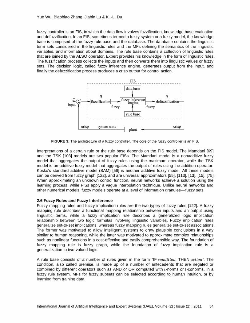
Yue Wu, Biaobiao Zhang, Jiabin Lu & K. -L. Du
International Journal of Artificial Intelligence and Expert Systems (IJAE), Volume (2) : Issue (2) : 2011 54
fuzzy controller is an FIS, in which the data flow involves fuzzification, knowledge base evaluation,
and defuzzification. In an FIS, sometimes termed a fuzzy system or a fuzzy model, the knowledge
base is comprised of the fuzzy rule base and the database. The database contains the linguistic
term sets considered in the linguistic rules and the MFs defining the semantics of the linguistic
variables, and information about domains. The rule base contains a collection of linguistic rules
that are joined by the ALSO operator. Expert provides his knowledge in the form of linguistic rules.
The fuzzification process collects the inputs and then converts them into linguistic values or fuzzy
sets. The decision logic, called fuzzy inference engine, generates output from the input, and
finally the defuzzification process produces a crisp output for control action.
FIGURE 3: The architecture of a fuzzy controller. The core of the fuzzy controller is an FIS.
Interpretations of a certain rule or the rule base depends on the FIS model. The Mamdani [69]
and the TSK [103] models are two popular FISs. The Mamdani model is a nonadditive fuzzy
model that aggregates the output of fuzzy rules using the maximum operator, while the TSK
model is an additive fuzzy model that aggregates the output of rules using the addition operator.
Kosko's standard additive model (SAM) [56] is another additive fuzzy model. All these models
can be derived from fuzzy graph [122], and are universal approximators [55], [113], [13], [15], [75].
When approximating an unknown control function, neural networks achieve a solution using the
learning process, while FISs apply a vague interpolation technique. Unlike neural networks and
other numerical models, fuzzy models operate at a level of information granules––fuzzy sets.
2.6 Fuzzy Rules and Fuzzy Interference
Fuzzy mapping rules and fuzzy implication rules are the two types of fuzzy rules [122]. A fuzzy
mapping rule describes a functional mapping relationship between inputs and an output using
linguistic terms, while a fuzzy implication rule describes a generalized logic implication
relationship between two logic formulas involving linguistic variables. Fuzzy implication rules
generalize set-to-set implications, whereas fuzzy mapping rules generalize set-to-set associations.
The former was motivated to allow intelligent systems to draw plausible conclusions in a way
similar to human reasoning, while the latter was motivated to approximate complex relationships
such as nonlinear functions in a cost-effective and easily comprehensible way. The foundation of
fuzzy mapping rule is fuzzy graph, while the foundation of fuzzy implication rule is a
generalization to two-valued logic.
A rule base consists of a number of rules given in the form ―IF 𝑐𝑜𝑛𝑑𝑖𝑡𝑖𝑜𝑛, THEN 𝑎𝑐𝑡𝑖𝑜𝑛”. The
condition, also called premise, is made up of a number of antecedents that are negated or
combined by different operators such as AND or OR computed with 𝑡-norms or 𝑡-conorms. In a
fuzzy rule system, MFs for fuzzy subsets can be selected according to human intuition, or by
learning from training data.
Yue Wu, Biaobiao Zhang, Jiabin Lu & K. -L. Du
International Journal of Artificial Intelligence and Expert Systems (IJAE), Volume (2) : Issue (2) : 2011 55
A fuzzy inference is made up of several rules with the same output variables. Given a set of fuzzy
rules, the inference result is a combination of the fuzzy values of the conditions and the
corresponding actions. For example, we have a set of 𝑁r rules
R𝑖: IF (𝑐𝑜𝑛𝑑𝑖𝑡𝑖𝑜𝑛 = 𝐶𝑖) THEN (𝑎𝑐𝑡𝑖𝑜𝑛 = 𝐴𝑖)
for 𝑖 = 1, … , 𝑁r , where 𝐶𝑖 is a fuzzy set. Assuming that a condition has a membership degree of 𝜇𝑖
associated with the set 𝐶𝑖 . The condition is first converted into a fuzzy category using a
syntactical representation, 𝑐𝑜𝑛𝑑𝑖𝑡𝑖𝑜𝑛 = 𝐶𝑖
𝜇 𝑖
𝑁r𝑖 . We can see each rule is valid to a certain extent. A
fuzzy inference is the combination of all the possible consequences. The action coming from a
fuzzy inference is also a fuzzy category, with a syntactical representation
𝑎𝑐𝑡𝑖𝑜𝑛 =𝐴1
𝜇1+
𝐴2
𝜇2+ ⋯ +
𝐴𝑁r
𝜇𝑁r
. (25)
The inference procedure depends on fuzzy reasoning. This result can be further processed or
transformed into a crisp value.
2.7 Fuzzification and Defuzzification
Fuzzification is to transform crisp inputs into fuzzy subsets. Given crisp inputs 𝑥𝑖 , 𝑖 = 1, … , 𝑛,
fuzzification is to construct the same number of fuzzy sets 𝐴𝑖,
𝐴𝑖 = fuzz 𝑥𝑖 , (26)
where fuzz ⋅ is a fuzzification operator. Fuzzification is determined according to the defined MFs.
Defuzzification is to map fuzzy subsets of real numbers into real numbers. In an FIS,
defuzzification is applied after aggregation. Popular defuzzification methods include the centroid
defuzzifier [69], and the mean-of-maxima defuzzifier [69]. The centroid defuzzifier is the best-
known method, which is to find the centroid of the area surrounded by the MF and the horizontal
axis [52]. Aggregation and defuzzification can be combined into a single phase, such as the
weighted-mean method [36]
defuzz 𝐵 = 𝜇𝑖𝑏𝑖
𝑁r𝑖=1
𝜇𝑖𝑁r𝑖=1
, (27)
where 𝑁r is the number of rules, 𝜇𝑖 is the degree of activation of the 𝑖th rule, and 𝑏𝑖 is a numeric
value associated with the consequent of the 𝑖th rule, 𝐵𝑖. The parameter 𝑏𝑖 can be selected as the
mean value of the 𝛼-level set when 𝛼 is equal to 𝜇𝑖 [36].
2.8 Mamdani Model
Given a set of 𝑁 examples 𝐱𝑝 , 𝐲𝑝 𝐱𝑝 ∈ 𝑅𝑛 , 𝐲𝑝 ∈ 𝑅𝑚 , the underlying system can be identified by
using the Mamdani or the TSK model.
For the Mamdani model with 𝑁r rules, the 𝑖th rule is given by
R𝑖: IF 𝐱 is 𝐴𝑖, THEN 𝐲 is 𝐵𝑖
for 𝑖 = 1, … , 𝑁r , where 𝐴𝑖 = { 𝐴𝑖1, 𝐴𝑖
2, … , 𝐴𝑖𝑛 }, 𝐵𝑖 = 𝐵𝑖
1, 𝐵𝑖2, … , 𝐵𝑖
𝑚 , and 𝐴𝑖𝑗 and 𝐵𝑖
𝑘 are respectively
fuzzy sets that define an input and output space partitioning.
Yue Wu, Biaobiao Zhang, Jiabin Lu & K. -L. Du
International Journal of Artificial Intelligence and Expert Systems (IJAE), Volume (2) : Issue (2) : 2011 56
For an 𝑛-tuple input in the form of ―𝐱 is A′‖, the system output ― 𝐲 is B′‖ is characterized by
combining the rules according to
𝜇𝐵′ 𝐲 = 𝜇𝐴𝑖′ 𝐱 ∧ 𝜇𝐵𝑖
𝐲
𝑁r
𝑖=1
, (28)
where the fuzzy partitioning 𝐴′ = {𝐴′1, 𝐴′2, … , 𝐴′𝑛 } and 𝐵′ = { 𝐵′1, 𝐵′2, … , 𝐵′𝑚 } ,
𝜇𝐴𝑖′ 𝐱 = 𝜇𝐴′ 𝐱 ∧ 𝜇𝐴𝑖
𝐱 = 𝜇𝐴′ 𝑗 ∧ 𝜇𝐴𝑖
𝑗
𝑛
𝑖=1
. (29)
𝜇𝐴′ 𝐱 = 𝜇𝐴′ 𝑗𝑛𝑗 =1 and 𝜇𝐴𝑖
𝐱 = 𝜇𝐴𝑖
𝑗𝑛𝑗=1 being respectively the membership degrees of 𝐱 to the
fuzzy sets 𝐴′ and 𝐴𝑖, 𝜇𝐵𝑖 𝐲 = 𝜇
𝐵𝑖𝑘
𝑚𝑘=1 is the membership degree of 𝐲 to the fuzzy set 𝐵𝑖, 𝜇𝐴′
𝑖𝑗 is
the association between the 𝑗th input of 𝐴′ and the 𝑖th rule, 𝜇𝐵𝑖
𝑘 is the association between the 𝑘th
input of 𝐵 and the 𝑖th rule, ∧ is the intersection operator, and ∨ is the union operator.
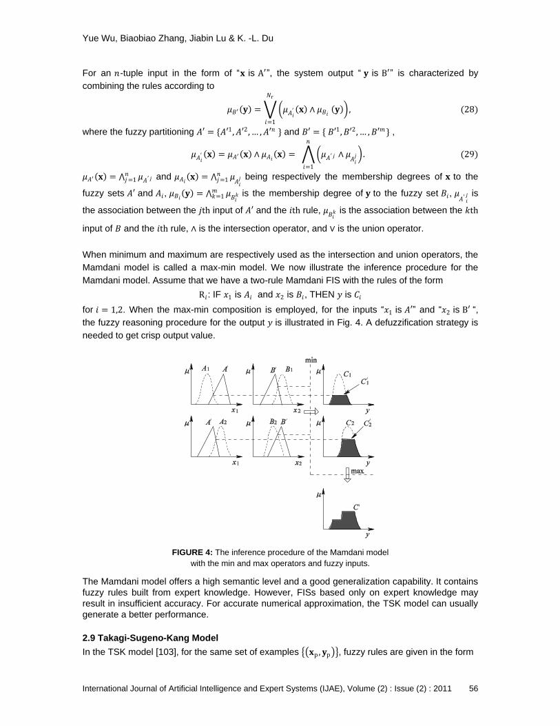
When minimum and maximum are respectively used as the intersection and union operators, the
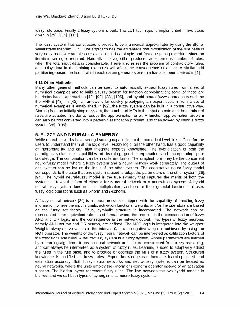
Mamdani model is called a max-min model. We now illustrate the inference procedure for the
Mamdani model. Assume that we have a two-rule Mamdani FIS with the rules of the form
R𝑖: IF 𝑥1 is 𝐴𝑖 and 𝑥2 is 𝐵𝑖, THEN 𝑦 is 𝐶𝑖
for 𝑖 = 1,2. When the max-min composition is employed, for the inputs ―𝑥1 is 𝐴′‖ and ―𝑥2 is B′ ―,
the fuzzy reasoning procedure for the output 𝑦 is illustrated in Fig. 4. A defuzzification strategy is
needed to get crisp output value.
FIGURE 4: The inference procedure of the Mamdani model
with the min and max operators and fuzzy inputs. The Mamdani model offers a high semantic level and a good generalization capability. It contains
fuzzy rules built from expert knowledge. However, FISs based only on expert knowledge may
result in insufficient accuracy. For accurate numerical approximation, the TSK model can usually
generate a better performance.
2.9 Takagi-Sugeno-Kang Model
In the TSK model [103], for the same set of examples 𝐱p , 𝐲p , fuzzy rules are given in the form
Yue Wu, Biaobiao Zhang, Jiabin Lu & K. -L. Du
International Journal of Artificial Intelligence and Expert Systems (IJAE), Volume (2) : Issue (2) : 2011 57
R𝑖: IF 𝐱 is 𝐴𝑖, THEN 𝐲 = 𝐟𝑖(𝐱)
for 𝑖 = 1,2, … , 𝑁r, where 𝐟𝑖 𝐱 = 𝑓𝑖1 𝐱 , … , 𝑓𝑖
𝑚 𝐱 𝑇
is a crisp vector function of 𝐱; usually 𝑓𝑖𝑗 𝐱 is
selected as a linear relation with 𝑓𝑖𝑗 𝐱 = 𝐚𝑖
𝑗 𝑇𝐱 + 𝑏𝑖
𝑗, where 𝐚𝑖
𝑗 and 𝑏𝑖
𝑗 are adjustable parameters.
For an 𝑛-tuple input in the form of ―𝐱 is 𝐴′‖, the output 𝐲′ is obtained by combining the rules
according to
𝐲′ = 𝜇𝐴𝑖
′ 𝐱 𝐟𝑖(𝐱)𝑁r𝑖=1
𝜇𝐴𝑖′ 𝐱 𝑁r
𝑖=1
, (30)
where 𝜇𝐴𝑖′ 𝐱 is defined by (29), and can be derived by the procedure shown in the left part of Fig.
4. This model produces a real-valued function, and it is essentially a model-based fuzzy control
method. The stability analysis of the TSK model is given in [104]. The TSK model typically selects
𝑓𝑖𝑗 (⋅) as first-order polynomials, hence the model termed the first-order TSK model. When 𝑓𝑖
𝑗 (⋅)
are selected as constants, it is called the zero-order TSK model and can be regarded as a special
case of the Mamdani model.
In comparison with the Mamdani model, the TSK model, which is based on automatic learning
from the data, can accurately approximate a function using fewer rules. It has a stronger and
more flexible representation capability than the Mamdani mode. In the TSK model, rules are
extracted from the data, but the generated rules may have no meaning for experts. The TSK
model has found more successful applications in building fuzzy systems.
2.10 Complex Fuzzy Logic
Complex fuzzy sets and logic are mathematical extensions of fuzzy sets and logic from the real
domain to the complex domain [87], [86]. A complex fuzzy set 𝑆 is characterized by a complex-
valued MF, and membership of any element 𝑥 in 𝑆 is given by a complex-valued membership
degree of the form
𝜇𝑆 𝑥 = 𝑟𝑆 𝑥 ej𝜑𝑆(𝑥), (31)
where the amplitude 𝑟𝑆 𝑥 ∈ [0,1], and 𝜑𝑆 is the phase. Thus, 𝜇𝑆 𝑥 is within a unit circle in the
complex plane.
In [87], [86], basic set operators for fuzzy logic have been extended for the complex fuzzy logic,
and some additional operators such as the vector aggregation, set rotation and set reflection, are
also defined. The operations of intersection, union and complement for complex fuzzy sets are
defined only on the modulus of the complex membership degree. In [27], the complex fuzzy logic
is extended to a logic of vectors in the plane, rather than scalar quantities. In [74], a complex
fuzzy set is defined as an MF mapping the complex plane into 0,1 × [0,1].
Complex fuzzy sets are superior to the Cartesian products of two fuzzy sets. Complex fuzzy logic
maintains both the advantages of the fuzzy logic and the properties of complex fuzzy sets. In
complex fuzzy logic, rules constructed are strongly related and a relation manifested in the phase
term is associated with complex fuzzy implications. In a complex FIS, the output of each rule is a
complex fuzzy set, and phase terms are necessary when combining multiple rules so as to
generate the final output. Complex FISs are useful for solving some hard problems for traditional
fuzzy methods, in which rules are related to one another with the nature of the relation varying as
a function of the input to the system [86].
The fuzzy complex number [11], introduced by incorporating the complex number into the support
of the fuzzy set, is a different concept from the complex fuzzy set [87]. A fuzzy complex number is
Yue Wu, Biaobiao Zhang, Jiabin Lu & K. -L. Du
International Journal of Artificial Intelligence and Expert Systems (IJAE), Volume (2) : Issue (2) : 2011 58
a fuzzy set of complex numbers, which have real-valued membership degree in the range [0,1]. An 𝛼-cut of a fuzzy complex number is based on the modulus of the complex numbers in the
fuzzy set. A fuzzy complex number is a fuzzy set in one dimension, while a complex fuzzy set or
number is a fuzzy set in two dimensions.
3. FUZZY LOGIC VS. NEURAL NETWORKS Like FNNs, many fuzzy systems are proved to be universal approximators [63], [50], [13], [35],
[57], [118]. In [63], the Mamdani model and FNNs are shown to be able to approximate each
other to an arbitrary accuracy. The equivalence between the TSK model and the RBFN under
certain conditions has been established in [50], [43] and the equivalence between fuzzy expert
systems and neural networks has been proved in [13]. Gaussian-based Mamdani systems have
the ability of approximating any sufficiently smooth function and reproducing its derivatives up to
any order [35]. In [57], fuzzy systems with Gaussian MFs have been proved to be universal
approximators for a smooth function and its derivatives.
From the viewpoint of an expert system, fuzzy systems and neural networks are quite similar as
inference systems. An inference system involves knowledge representation, reasoning, and
knowledge acquisition: (1) A trained neural network represents knowledge using connection
weights and neurons in a distributed manner, while in a fuzzy system knowledge is represented
using IF-THEN rules; (2) For each input, the trained neural network generates an output and this
pure numerical procedure can be treated as a reasoning process, while reasoning in a fuzzy
system is logic-based; (3) Knowledge acquisition is via learning in a neural network, while for a
fuzzy system knowledge is encoded by a human expert. Both neural networks and fuzzy systems
are dynamic, parallel distributed processing systems that estimate functions without any
mathematical model and learn from experience with sample data.
Fuzzy systems can be applied to problems with knowledge represented in the form of IF-THEN
rules. Problem-specific a priori knowledge can be integrated into the systems. Training pattern set
and system modeling are not needed, and only heuristics are used. During the tuning process,
one needs to add, remove, or change a rule, or even change the weight of a rule. This process,
however, requires the knowledge of experts. On the other hand, neural networks are useful when
we have training pattern set. We do not need any knowledge of the modeling of the problem. A
trained neural network is a black box that represents knowledge in its distributed structure.
However, any prior knowledge of the problem cannot be incorporated into the learning process. It
is difficult for human beings to understand the internal logic of the system. Nevertheless, by
extracting rules from neural networks, users can understand what neural networks have learned
and how neural networks predict.
4. FUZZY INFERENCE SYSTEMS AND NEURAL NETWORKS
4.1 Fuzzy Inference Systems and Multilayer Perceptrons
For a three-layer (𝐽1-𝐽2-𝐽3) MLP, if the activation function in the hidden layer 𝜙(1)(⋅) is selected as
the logistic function 𝜙 1 𝑥 =1
1+e−𝑥 and the activation function in the output layer 𝜙(2)(⋅) is
selected as the linear function 𝜙(2)(𝑥) = 𝑥 , there always exists a fuzzy additive system that
calculates the same function as the network does [7]. In [7], a fuzzy logic operator, called
interactive-or (𝑖-or), is defined by applying the concept of 𝑓-duality to the logistic function. The use
of the 𝑖-or operator explains clearly the acquired knowledge of a trained MLP. The 𝑖-or operator is
defined by [7]
Yue Wu, Biaobiao Zhang, Jiabin Lu & K. -L. Du
International Journal of Artificial Intelligence and Expert Systems (IJAE), Volume (2) : Issue (2) : 2011 59
𝑎 ⊗ 𝑏 = 𝑎⋅ 𝑏
1−𝑎 ⋅ 1−𝑏 +𝑎⋅ 𝑏. (32)
The 𝑖-or operator works on (0,1). It is a hybrid between both a 𝑡-norm and a 𝑡-conorm. Based on
the 𝑖-or operator, the equality between MLPs and FISs is thus established [7]. The equality proof
also yields an automated procedure for knowledge acquisition. An extension of the method has
been presented in [16], where the fuzzy rules obtained are in agreement with the domain of the
input variables and a new logical operator, similar to, but with a higher representational power
than the 𝑖-or, is defined.
In [32], relations between input uncertainties and fuzzy rules have been established. Sets of crisp
logic rules applied to uncertain inputs are shown to be equivalent to fuzzy rules with sigmoidal
MFs applied to crisp inputs. Integration of a reasonable uncertainty distribution for a fixed rule
threshold or interval gives a sigmoidal MF. Crisp logic and fuzzy rule systems are shown to be
respectively equivalent to the logical network and the three-layer MLP. Keeping fuzziness on the
input side enables easier understanding of the networks or the rule systems. In [17], [100], MLPs
are interpreted by fuzzy rules in such a way that the sigmoidal activation function is decomposed
into three partitions, and represented by three TSK fuzzy rules with one TSK fuzzy rule for each
partition. Each partition has its own MF. Accordingly, the value of the activation function at a point
can be derived by the TSK model.
A fuzzy set is usually represented by a finite number of its supports. In comparison with
conventional MF based FISs, 𝛼-cut based FISs [109] have a number of advantages. They can
considerably reduce the required memory and time complexity, since they depend on the number
of membership-grade levels, and not on the number of elements in the universes of discourse.
Secondly, the inference operations can be performed for each 𝛼-cut set independently, and this
enables parallel implementation. An 𝛼-cut based FIS can also easily interface with two-valued
logic since the 𝛼-level sets themselves are crisp sets. In addition, fuzzy set operations based on
the extension principle can be performed efficiently using 𝛼-level sets [109], [64]. For 𝛼-cut based
FISs, each fuzzy rules can be represented as a pattern pair of degrees of membership at those
points of the MFs obtained by dividing the intervals of the fuzzy sets linearly or by 𝛼-cut can be
implemented by an MLP with the backpropagation (BP) rule. This is a learning problem of 𝑁r
samples with 𝑛 inputs and 𝑚 outputs.
4.2 Fuzzy Inference Systems and Radial Basis Function Networks
When the 𝑡-norm in the TSK model is selected as multiplication and the MFs are selected the
same as RBFs in the normalized RBFN model, the two models are mathematically equivalent [50],
[48]. Note that each hidden unit corresponds to a fuzzy rule. Normalized RBFNs provide a
localized solution that is amenable to rule extraction. The receptive fields of some RBFs should
overlap to prevent incompleteness of fuzzy partitions. To have a perfect match between the RBFs
𝜙 𝐱 − 𝐜𝑖 and 𝜇𝐴𝑖′ (𝐱) in (30), 𝜙 𝐱 − 𝐜𝑖 should be factorizable in each dimension such that
each component 𝜙 |𝑥𝑗 − 𝑐𝑖 ,𝑗 | corresponds to an MF 𝜇𝑨′
𝑗 . The Gaussian RBF is the only strictly
factorizable function.
In the normalized RBFN, 𝑤𝑖𝑗 ’s typically take constant values and the normalized RBFN
corresponds to the zero-order TSK model. When the RBF weights are linear regression functions
of the input variables [59], [91], the model is functionally equivalent to the first-order TSK model.
When implementing the TSK model, one can select some 𝜇𝐴′ 𝑖
𝑗 = 1 or some 𝜇𝐴′ 𝑖
𝑗 = 𝜇𝐴′𝑘
𝑗 in order to
Yue Wu, Biaobiao Zhang, Jiabin Lu & K. -L. Du
International Journal of Artificial Intelligence and Expert Systems (IJAE), Volume (2) : Issue (2) : 2011 60
increase the distinguishability of the fuzzy partitions. Correspondingly, one should share some
component RBFs or set some component RBFs to unity [52]. This considerably reduces the
effective number of free parameters in the RBFN. A distance measure like the Euclidean distance
is used to describe the similarity between two component RBFs. After applying a clustering
technique to locate prototypes and adding a regularization term describing the total similarity
between all the RBFs and the shared RBF to the MSE function, a gradient-descent procedure is
conducted so as to extract interpretable fuzzy rules from a trained RBFN [52]. The method can be
applied to RBFNs with constant or linear regression weights. A fuzzy system can be first
constructed according to heuristic knowledge and existing data, and then converted into an RBFN.
This is followed by a refinement of the RBFN using a learning algorithm. Due to this learning
procedure, the interpretability of the original fuzzy system may be lost. The RBFN is then again
converted into interpretable fuzzy system, and knowledge is extracted from the network. This
process refines the original fuzzy system design. The algorithm for rule extraction from the RBFN
is given in [52].
In [107], normalized Gaussian RBFNs can be generated from simple probabilistic rules and
probabilistic rules can also be extracted from trained RBFNs. Methods for reducing network
complexity have been presented in order to obtain concise and meaningful rules. Two algorithms
for rule extraction from RBFNs, which respectively generate a single rule describing each class
and a single rule from each hidden unit, are given in [70]. Existing domain knowledge in rule
format can be inserted into an RBFN as an initialization of optimal network training.
4.3 Rule Generation from Trained Neural Networks
In addition to rule generation from trained MLPs and RBFNs, rule generation can also be
performed on other trained neural networks [46], [106]). Rule generation involves rule extraction
and rule refinement. Rule extraction is to extract knowledge from trained neural networks, while
rule refinement is to refine the rules that are extracted from neural networks and initialized with
crude domain knowledge.
Recurrent neural networks (RNNs) have the ability to store information over indefinite periods of
time, develop hidden states through learning, and thus conveniently represent recursive linguistic
rules [72]. They are particularly well-suited for problem domains, where incomplete or
contradictory prior knowledge is available. In such cases, knowledge revision or refinement is
also possible. Discrete-time RNNs can correctly classify strings of a regular language [80]. Rules
defining the learned grammar can be extracted in the form of deterministic finite-state automata
(DFAs) by applying clustering algorithms [29] in the output space of neurons. Starting from an
initial network state, the algorithm searches the equally partitioned output space of 𝑁 state
neurons in a breadth-first manner. A heuristic is used to choose among the consistent DFAs that
model, which best approximates the learned regular grammar. The extracted rules demonstrate
high accuracy and fidelity and the algorithm is portable. Based on [80], an augmented RNN that
encodes fuzzy finite-state automata (FFAs) and recognizes a given fuzzy regular language with
an arbitrary accuracy has been constructed in [81]. FFAs are transformed into equivalent DFAs
by using an algorithm that computes fuzzy string membership. FFAs can model dynamical
processes whose current state depends on the current input and previous states. The granularity
within both extraction techniques is at the level of ensemble of neurons, and thus, the approaches
are not strictly decompositional.
RNNs are suitable for crisp/fuzzy grammatical inference. A method that uses a SOM for
extracting knowledge from an RNN [9] is able to infer a crisp/fuzzy regular language. Rule
extraction is also carried out upon Kohonen networks [110]. A comprehensive survey on rule
generation from trained neural networks is given from a softcomputing perspective in [72], where
the optimization capability of evolutionary algorithms (EAs) are emphasized for rule refinement.
Yue Wu, Biaobiao Zhang, Jiabin Lu & K. -L. Du
International Journal of Artificial Intelligence and Expert Systems (IJAE), Volume (2) : Issue (2) : 2011 61
Rule extraction from RNNs aims to find models of an RNN, typically in the form of finite state
machines. A recent overview of rule extraction from RNNs is given in [47].
4.4 Extracting Rules from Numerical Data
FISs can be designed directly from expert knowledge and data. The design process is usually
decomposed into two phases, namely, rule generation and system optimization [39]. Rule
generation leads to a basic system with a given space partitioning and the corresponding set of
rules, while system optimization gives the optimal membership parameters and rule base. Design
of fuzzy rules can be performed in one of three ways, namely, all the possible combinations of
fuzzy partitions, one rule for each data pair, or dynamically choosing the number of fuzzy sets.
For good interpretability, a suitable selection of variables and the reduction of the rule base are
necessary. During the system optimization phase, merging techniques such as cluster merging
and fuzzy set merging are usually used for interpretability purposes. Fuzzy set merging leads to a
higher interpretability than cluster merging. The reduction of a set of rules results in a loss of
numerical performance on the training data set, but a more compact rule base has a better
generalization capability and is also easier for human understanding. EAs [93] or learning [50] are
also used for extracting fuzzy rules and optimizing MFs and rule base. Methods for designing
FISs from data are analyzed and surveyed in [39]. They are grouped into several families and
compared based on rule interpretability.
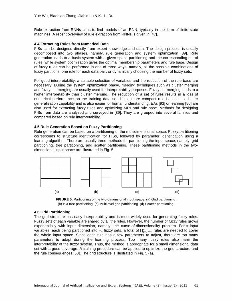
4.5 Rule Generation Based on Fuzzy Partitioning
Rule generation can be based on a partitioning of the multidimensional space. Fuzzy partitioning
corresponds to structure identification for FISs, followed by parameter identification using a
learning algorithm. There are usually three methods for partitioning the input space, namely, grid
partitioning, tree partitioning, and scatter partitioning. These partitioning methods in the two-
dimensional input space are illustrated in Fig. 5.
(a) (b) (c) (d)
FIGURE 5: Partitioning of the two-dimensional input space. (a) Grid partitioning.
(b) 𝑘-𝑑 tree partitioning. (c) Multilevel grid partitioning. (d) Scatter partitioning.
4.6 Grid Partitioning
The grid structure has easy interpretability and is most widely used for generating fuzzy rules.
Fuzzy sets of each variable are shared by all the rules. However, the number of fuzzy rules grows
exponentially with input dimension, namely, the curse-of-dimensionality problem. For 𝑛 input
variables, each being partitioned into 𝑚𝑖 fuzzy sets, a total of 𝑚𝑖𝑛𝑖=1 rules are needed to cover
the whole input space. Since each rule has a few parameters to adjust, there are too many
parameters to adapt during the learning process. Too many fuzzy rules also harm the
interpretability of the fuzzy system. Thus, the method is appropriate for a small dimensional data
set with a good coverage. A training procedure can be applied to optimize the grid structure and
the rule consequences [50]. The grid structure is illustrated in Fig. 5 (a).
Yue Wu, Biaobiao Zhang, Jiabin Lu & K. -L. Du
International Journal of Artificial Intelligence and Expert Systems (IJAE), Volume (2) : Issue (2) : 2011 62
4.7 Tree Partitioning
𝑘-𝑑 tree and multilevel grid structures are two hierarchical partitioning techniques that effectively
relieve the problem of rule explosion [101]. The input space is first partitioned roughly, and a
subspace is recursively divided until a desired approximation performance is achieved. The 𝑘-𝑑
tree results from a series of guillotine cuts. A guillotine cut is a cut that is entirely across the
subspace to be partitioned. After the 𝑖th guillotine cut, the entire space is partitioned into 𝑖 + 1
regions. Heuristics based on the distribution of training examples or parameter identification
methods can usually be employed to find a proper 𝑘-𝑑 tree structure [101]. For the multilevel grid
structure [101], the top-level grid coarsely partitions the whole space into equal-sized and evenly
spaced fuzzy boxes, which are recursively partitioned into finer grids until a criterion is met.
Hence, a multilevel grid structure is also called a box tree. The criterion can be that the resulting
boxes have similar number of training examples or that an application-specific evaluation in each
grid is below a threshold. A 𝑘-𝑑 tree partitioning and a multilevel grid partitioning are respectively
illustrated in Fig. 5 (b) and (c). A multilevel grid in the two-dimensional space is called a quad tree.
Tree partitioning needs some heuristics to extract rules and its application to high-dimensional
problems faces practical difficulties.
4.8 Scatter Partitioning
Scatter partitioning usually generates fewer fuzzy regions than the grid and tree partitioning
techniques owing to the natural clustering property of training patterns. Fuzzy clustering
algorithms form a family of rule generation techniques. The training examples are gathered into
homogeneous groups and a rule is associated to each group. The fuzzy sets are not shared by
the rules, but each of them is tailored for one particular rule. Thus, the resulting fuzzy sets are
usually difficult to interpret [39]. Clustering is well adapted for large work spaces with a small
amount of training examples. However, scatter partitioning of high-dimensional feature spaces is
difficult, and some learning or evolutionary procedures may be necessary. Clustering algorithms
[29] can be applied for scatter partitioning. A scatter partitioning is illustrated in Fig. 5 (d). The
curse of dimensionality can also be alleviated by reducing the input dimensions by discarding
some irrelevant inputs or compressing the input space using feature selection or feature
extraction techniques. Some clustering-based methods for extracting fuzzy rule for function
approximation are proposed in [121], [20], [21], [4]. These methods are based on the TSK model.
Clustering can be used for identification of the antecedent part of the model such as
determination of the number of rules and initial rule parameters. The consequent part of the
model can be estimated by the linear LS method. In [21], the combination of the subtractive
clustering with the linear LS method provides an extremely fast and accurate method for fuzzy
system identification, which is better than the adaptive-network-based FIS (ANFIS) [48]. Based
on the Mamdani model, a clustering-based method for nonlinear regression is also given in [117].
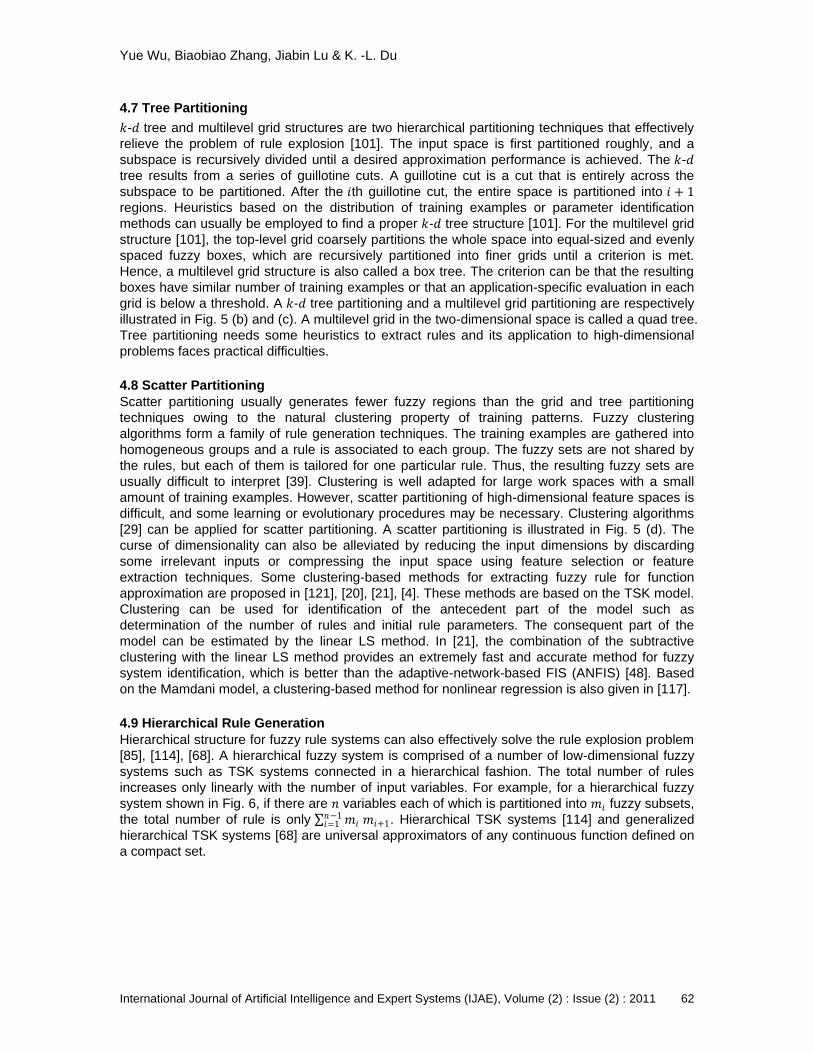
4.9 Hierarchical Rule Generation
Hierarchical structure for fuzzy rule systems can also effectively solve the rule explosion problem
[85], [114], [68]. A hierarchical fuzzy system is comprised of a number of low-dimensional fuzzy
systems such as TSK systems connected in a hierarchical fashion. The total number of rules
increases only linearly with the number of input variables. For example, for a hierarchical fuzzy
system shown in Fig. 6, if there are 𝑛 variables each of which is partitioned into 𝑚𝑖 fuzzy subsets,
the total number of rule is only 𝑚𝑖 𝑚𝑖+1𝑛−1𝑖=1 . Hierarchical TSK systems [114] and generalized
hierarchical TSK systems [68] are universal approximators of any continuous function defined on
a compact set.
Yue Wu, Biaobiao Zhang, Jiabin Lu & K. -L. Du
International Journal of Artificial Intelligence and Expert Systems (IJAE), Volume (2) : Issue (2) : 2011 63
FIGURE 6: Example of a hierarchical fuzzy system with 𝑛 inputs and one output. The system is comprised
of 𝑛 − 1 two-input TSK systems. The 𝑛 input variables are 𝑥𝑖 , 𝑖 = 1, … , 𝑛,
the output is denoted by 𝑦, and 𝑦𝑖 is the output of the 𝑖th TSK system.
In Fig. 6, the 𝑛 input variables are 𝑥𝑖 , 𝑖 = 1, … , 𝑛, and the output is denoted by 𝑦. There exist
relations
𝑦𝑖 = 𝑓𝑖 𝑦𝑖−1, 𝑥𝑖+1 (33)
for 𝑖 = 1, … , 𝑛 − 1, where 𝑓𝑖 is the nonlinear relation described by the 𝑖th TSK system, 𝑦𝑖 is the
output of the 𝑖th TSK system, and 𝑦0 = 𝑥1. The final output is 𝑦 = 𝑦𝑛−1. The output 𝑦 is easily
obtained by a recursive procedure. Thus, the inference in the hierarchical fuzzy system is in a
recursive manner.
The hierarchical fuzzy system reduces the number of rules, however, the curse of dimensionality
is inherent in the system. In the standard fuzzy system, the degree of freedom is unevenly
distributed over the IF and THEN parts of the rules, with a comprehensive IF part to cover the
whole domain and a simple THEN part. The hierarchical fuzzy system, on the other hand,
provides with an incomplete IF part but a more complex THEN part. The gradient-descent method
can be applied to parameter learning of these systems. Generally, conventional fuzzy systems
achieve universal approximation using piecewise-linear functions, while the hierarchical fuzzy
system achieves it through piecewise-polynomial functions [114], [68].
4.10 Rule Generation Based on Look-up Table
Designing fuzzy systems from pattern pairs is a nonlinear regression problem. In the simple look-
up table (LUT) technique [115], [117], each pattern pair generates one fuzzy rule and then a
selection process determines the important rules, which are used to construct the final fuzzy
system. In the LUT technique, the input MFs do not change with the sampling data, thus the
designed fuzzy system uniformly covers the domain of interest.
In the LUT technique, the input and output spaces are first divided into fuzzy regions, then a fuzzy
rule is generated from a given pattern pair, and finally a degree is assigned to each rule to
resolve rule conflicts and reduce the number of rules. When the number of examples is large,
there is a high probability of conflicting rules, i.e., rules with the same IF parts but different THEN
parts. Each rule is assigned a degree of fulfillment. For a group of conflicting rules, only the rule
with the maximum degree is retained. When a new pattern pair becomes available, a rule is
created for this pattern pair and the fuzzy rule base is updated. The generated rules as well as
human expert's knowledge in the form of linguistic rules can be combined so as to produce a
Yue Wu, Biaobiao Zhang, Jiabin Lu & K. -L. Du
International Journal of Artificial Intelligence and Expert Systems (IJAE), Volume (2) : Issue (2) : 2011 64
fuzzy rule base. Finally a fuzzy system is built. The LUT technique is implemented in five steps
given in [29], [115], [117].
The fuzzy system thus constructed is proved to be a universal approximator by using the Stone-
Weierstrass theorem [115]. The approach has the advantage that modification of the rule base is
very easy as new examples are available. It is a simple and fast one-pass procedure, since no
iterative training is required. Naturally, this algorithm produces an enormous number of rules,
when the total input data is considerable. There also arises the problem of contradictory rules,
and noisy data in the training examples will affect the consequence of a rule. A similar grid
partitioning-based method in which each datum generates one rule has also been derived in [1].
4.11 Other Methods
Many other general methods can be used to automatically extract fuzzy rules from a set of
numerical examples and to build a fuzzy system for function approximation; some of these are
heuristics-based approaches [42], [92], [28], [105], and hybrid neural-fuzzy approaches such as
the ANFIS [48]. In [42], a framework for quickly prototyping an expert system from a set of
numerical examples is established. In [92], the fuzzy system can be built in a constructive way.
Starting from an initially simple system, the number of MFs in the input domain and the number of
rules are adapted in order to reduce the approximation error. A function approximation problem
can also be first converted into a pattern classification problem, and then solved by using a fuzzy
system [28], [105].
5. FUZZY AND NEURAL: A SYNERGY While neural networks have strong learning capabilities at the numerical level, it is difficult for the
users to understand them at the logic level. Fuzzy logic, on the other hand, has a good capability
of interpretability and can also integrate expert's knowledge. The hybridization of both the
paradigms yields the capabilities of learning, good interpretation and incorporating prior
knowledge. The combination can be in different forms. The simplest form may be the concurrent
neuro-fuzzy model, where a fuzzy system and a neural network work separately. The output of
one system can be fed as the input of the other system. The cooperative neuro-fuzzy model
corresponds to the case that one system is used to adapt the parameters of the other system [38],
[94]. The hybrid neural-fuzzy model is the true synergy that captures the merits of both the
systems. It takes the form of either a fuzzy neural network or a neuro-fuzzy system. A hybrid
neural-fuzzy system does not use multiplication, addition, or the sigmoidal function, but uses
fuzzy logic operations such as 𝑡-norm and 𝑡-conorm.
A fuzzy neural network [84] is a neural network equipped with the capability of handling fuzzy
information, where the input signals, activation functions, weights, and/or the operators are based
on the fuzzy set theory. Thus, symbolic structure is incorporated. The network can be
represented in an equivalent rule-based format, where the premise is the concatenation of fuzzy
AND and OR logic, and the consequence is the network output. Two types of fuzzy neurons,
namely AND neuron and OR neuron, are defined. The NOT logic is integrated into the weights.
Weights always have values in the interval [0,1], and negative weight is achieved by using the
NOT operator. The weights of the fuzzy neural network can be interpreted as calibration factors of
the conditions and rules. A neuro-fuzzy system is a fuzzy system, whose parameters are learned
by a learning algorithm. It has a neural network architecture constructed from fuzzy reasoning,
and can always be interpreted as a system of fuzzy rules. Learning is used to adaptively adjust
the rules in the rule base, and to produce or optimize the MFs of a fuzzy system. Structured
knowledge is codified as fuzzy rules. Expert knowledge can increase learning speed and
estimation accuracy. Both fuzzy neural networks and neuro-fuzzy systems can be treated as
neural networks, where the units employ the 𝑡-norm or 𝑡-conorm operator instead of an activation
function. The hidden layers represent fuzzy rules. The line between the two hybrid models is
blurred, and we call both types of synergisms as neuro-fuzzy systems.
Yue Wu, Biaobiao Zhang, Jiabin Lu & K. -L. Du
International Journal of Artificial Intelligence and Expert Systems (IJAE), Volume (2) : Issue (2) : 2011 65
Neuro-fuzzy systems can be obtained by representing some of the parameters of a neural
network, such as the inputs, weights, outputs, and shift terms as continuous fuzzy numbers.
When only the input is fuzzy, it is a Type I neuro-fuzzy system. When everything except the input
is fuzzy, we get a Type II model. A type III model is defined as one where the inputs, weights, and
shift terms are all fuzzy. The functions realizing the inference process, such as 𝑡-norm and 𝑡-
conorm, are usually nondifferentiable. To utilize gradient-based algorithms, one has to select
differential functions for the inference functions. For nondifferentiable inference functions, training
can be performed by using EAs. The shape of the MFs, the number of fuzzy partitions, and rule
base can all be evolved by using EAs. The neuro-fuzzy method is superior to the neural network
method in terms of the convergence speed and compactness of the structure. Fundamentals in
neuro-fuzzy synergism for modeling and control have been reviewed in [51].
5.1 Interpretability
Interpretability is one major reason for using fuzzy systems. Interpretability helps to check the
plausibility of a system, leading to easy maintenance of the system. It can also be used to acquire
knowledge from a problem characterized by numerical examples. An improvement in
interpretability can enhance the performance of generalization when the data set is small. The
interpretability of a rule base is usually related to continuity, consistency and completeness [39].
Continuity guarantees that small variations of the input do not induce large variations in the output.
Consistency means that if two or more rules are simultaneously fired, their conclusions are
coherent. Completeness means that for any possible input vector, at least one rule is fired and
there is no inference breaking.
When neuro-fuzzy systems are used to model nonlinear functions described by training sets, the
approximation accuracy can be optimized by the learning procedure. However, since learning is
accuracy-oriented, it usually causes a reduction in the interpretability of the generated fuzzy
system. The loss of interpretability can be due to incompleteness of fuzzy partitions,
indistinguishability of fuzzy partitions, inconsistancy of fuzzy rules, too fuzzy or too crisp fuzzy
subsets, or incompactness of the fuzzy system [52]. To improve the interpretability of neuro-fuzzy
systems, one can add to the cost function, regularization terms that apply constraints on the
parameters of fuzzy MFs. For example, the order of the 𝐿 centers of the fuzzy subset 𝐴𝑗 (𝑥),
𝑗 = 1, … , 𝐿, should be specified and remain unchanged during learning. Similar MFs should be
merged to improve the distinguishability of fuzzy partitions and to reduce the number of fuzzy
subsets [96]. One can also reduce the number of free parameters in defining fuzzy subsets. To
increase the interpretability of the designed fuzzy system, the same linguistic term should be
represented by the same MF. This results in weight sharing [75], [52]. For the TSK model, one
practice for good interpretability is to keep the number of fuzzy subsets much smaller than 𝑁r, the
number of fuzzy rules, especially when 𝑁r is large.
6. NEURO-FUZZY MODELS A typical architecture of a neuro-fuzzy system includes an input layer, an output layer, and
several hidden layers. The weights are fuzzy sets, and the neurons apply 𝑡-norm or 𝑡-conorm
operations. The hidden layers are usually used as rule layers. The layers before the rule layers
perform as premise layers, while those after perform as consequent layers. A well-known neuro-
fuzzy model is the ANFIS model [48]. We describe the ANFIS model in this section and also give
a brief survey of neuro-fuzzy models.
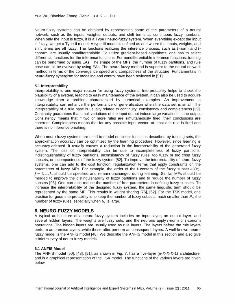
6.1 ANFIS Model
The ANFIS model [50], [48], [51], as shown in Fig. 7, has a five-layer (𝑛-𝐾-𝐾-𝐾-1) architecture,
and is a graphical representation of the TSK model. The functions of the various layers are given
below.
Yue Wu, Biaobiao Zhang, Jiabin Lu & K. -L. Du
International Journal of Artificial Intelligence and Expert Systems (IJAE), Volume (2) : Issue (2) : 2011 66
FIGURE 7: ANFIS: graphical representation of the TSK model. The symbol N in the circles denotes the
normalization operator, and 𝐱 = 𝑥1, 𝑥2, … , 𝑥𝑛 𝑇 .
Layer 1 is the input layer with 𝑛 nodes. The weights between the first two layers, 𝑤𝑖𝑗 = 𝜇𝐴𝑗
𝑖 (𝑥𝑖),
𝑖 = 1, … , 𝑛, 𝑗 = 1, … , 𝐾, denotes membership values of the 𝑖th input (antecedent) of the 𝑗th rule,
where 𝐴𝑗𝑖 corresponds to a partition of the space of 𝑥𝑖 , and 𝜇
𝐴𝑗𝑖 (𝑥𝑖) is typically selected as a
generalized bell MF 𝜇𝐴𝑗
𝑖 𝑥𝑖 = 𝜇(𝑥𝑖 ; 𝑐𝑖𝑗, 𝑎𝑖
𝑗, 𝑏𝑖
𝑗), where 𝑐𝑖
𝑗, 𝑎𝑖
𝑗, and 𝑏𝑖
𝑗 are referred to as premise
parameters. Layer 2 has 𝐾 fuzzy neurons with the product 𝑡-norm as the aggregation operator.
Each node corresponds to a rule, and the output of the 𝑗th neuron determines the degree of
fulfillment of the 𝑗th rule
𝑜𝑗(2)
= 𝜇𝐴𝑗
𝑖 𝑥𝑖 (34)
𝑛
𝑖=1
for 𝑗 = 1, … , 𝐾 . Each neuron in layer 3 performs normalization, and the outputs are called
normalized firing strengths
𝑜𝑗(3)
=𝑜𝑗
(2)
𝑜𝑘(2)𝐾
𝑘=1
(35)
for 𝑗 = 1, … , 𝐾. The output of each node in layer 4 is defined by
𝑜𝑗(4)
= 𝑜𝑗(3)
𝑓𝑗 (𝐱) (36)
for 𝑗 = 1, … , 𝐾. Parameters in 𝑓𝑗 (𝐱) are referred to as consequent parameters. The outputs of
layer 4 are summed and the output of the network gives the TSK model (30)
𝑜(5) = 𝑜𝑗(4)
𝐾
𝑗 =1
. (37)
In the ANFIS model, functions used at all the nodes are differentiable, thus the BP algorithm can
be used to learn the premise parameters by using a sample set of size 𝑁 , {(𝐱𝑡 , 𝑦𝑡)} . The
effectiveness of the model is dependent on the MFs used. The TSK fuzzy rules are employed in
the ANFIS model
R𝑖: IF 𝐱 is 𝐴𝑖, THEN 𝑦 = 𝑓𝑖 𝐱 = 𝑎𝑖 ,𝑗 𝑥𝑗 + 𝑎𝑖 ,0𝑛𝑗 =1
Yue Wu, Biaobiao Zhang, Jiabin Lu & K. -L. Du
International Journal of Artificial Intelligence and Expert Systems (IJAE), Volume (2) : Issue (2) : 2011 67
for 𝑖 = 1, … , 𝐾 , where 𝐴𝑖 = 𝐴𝑖1, 𝐴𝑖
2, … , 𝐴𝑖𝑛 are fuzzy sets and 𝑎𝑖 ,𝑗 , 𝑗 = 0, 1, … , 𝑛 , are consequent
parameters. The output of the network at time 𝑡 is thus given by
𝑦 𝑡 = 𝜇𝐴𝑖
𝐱𝑡 𝑓𝑖(𝐱𝑡)𝐾𝑖=1
𝜇𝐴𝑖 𝐱𝑡
𝐾𝑖=1
, (38)
where 𝜇𝐴𝑖 𝐱𝑡 = 𝜇
𝐴𝑗𝑖 (𝑥𝑡 ,𝑗 )𝑛
𝑗=1 . Accordingly, the error measure at time 𝑡 is defined by 𝐸𝑡 =
1
2 𝑦 𝑡 − 𝑦𝑡
2.
After the rule base is specified, the ANFIS adjusts only the MFs of the antecedents and the
consequent parameters. The BP algorithm can be used to train both the premise and consequent
parameters. A more efficient procedure is to learn the premise parameters by the BP, but to learn
the linear consequent parameters by the RLS method [48]. The learning rate 𝜂 can be adaptively
adjusted by some heuristics. It is reported in [48] that this hybrid learning method provides better
results than the MLP trained by the BP method and the cascade-correlation network [34]. In [49],
the Levenberg-Marquardt (LM) method [29] is used for ANFIS training. Compared to the hybrid
method, the LM method achieves a better precision, but the interpretability of the final MFs is
quite weak. In [18], the RProp [89] and the RLS methods are used to learn the premise
parameters and the consequent parameters, respectively. The ANFIS model has been
generalized for classification by employing parameterized 𝑡-norms [101], where tree partitioning is
used for structure identification and the Kalman filtering method for parameter learning.
The ANFIS is attractive for applications in view of its network structure and the standard learning
algorithm. Training of the ANFIS follows the spirit of the minimal disturbance principle and is thus
more efficient than the MLP [51]. However, the ANFIS is computationally expensive due to the
curse-of-dimensionality problem arising from grid partitioning. Tree or scattering partitioning can
resolve the curse of dimensionality, but leads to a reduction in the interpretability of the generated
rules. Constraints on MFs and initialization using prior knowledge cannot be provided to the
ANFIS model due to the learning procedure. The learning results may be difficult to interpret.
Thus, the ANFIS model is suitable for applications, where performance is more important than
interpretation. In order to preserve the plausibility of the ANFIS, one can add some regularization
terms to the cost function so that some constraints on the interpretability are considered [51].
The ANFIS has been extended to the coactive ANFIS [73] and to the generalized ANFIS [5]. The
coactive ANFIS [73] is a generalization of the ANFIS by introducing nonlinearity into the TSK
rules. The generalized ANFIS [5] is based on a generalization of the TSK model and a
generalized Gaussian RBFN. The generalized fuzzy model is trained by using the generalized
RBFN model, based on the functional equivalence between the two models. The sigmoid-ANFIS
[125] employs only sigmoidal MFs and adopts the interactive-or operator [7] as its fuzzy
connectives. The gradient-descent algorithm can also be directly applied to the TSK model
without representing it in a network structure [77]. The unfolding-in-time [119] is a method to
transform an RNN into an FNN so that the BP algorithm can be used. The ANFIS-unfolded-in-
time [99] is designed for prediction of time series data, and achieves much smaller error in the
ANFIS-unfolded-in-time compared to that in the ANFIS.
6.2 Generic Fuzzy Perceptron
The generic fuzzy perceptron (GFP) [75] has a structure similar to that of the three-layer MLP.
The network inputs and the weights are modeled as fuzzy sets, and 𝑡-norm or 𝑡-conorm is used
as the activation function at each unit. The hidden layer acts as the rule layer. The output units
usually use a defuzzufication function. The GFP can interpret its structure in the form of linguistic
rules and the structure of the GFP can be treated as a linguistic rule base, where the weights
between the input and hidden (rule) layers are called fuzzy antecedent weights and the weights

Yue Wu, Biaobiao Zhang, Jiabin Lu & K. -L. Du
International Journal of Artificial Intelligence and Expert Systems (IJAE), Volume (2) : Issue (2) : 2011 68
between the hidden (rule) and output layers fuzzy consequent weights. The GFP model is based
on the Mamdani model.
The NEFCON [76], [75], [78], NEFCLASS [75], and NEFPROX [75] models are three neuro-fuzzy
models based on the GFP model, which are used for control, classification and approximation,
respectively. Due to the use of nondifferentiable 𝑡 -norm and 𝑡 -conorm, the gradient-descent
method cannot be applied. A set of linguistic rules are used for describing the performance of the
models. This knowledge-based fuzzy error is independent of the range of the output value.
Learning algorithms for all these models are derived from the fuzzy error using simple heuristics.
Initial fuzzy partitions are needed to be specified for each input variable. Some connections that
have identical linguistic values are forced to have the same weights so as to keep the
interpretability. Prior knowledge can be integrated in the form of fuzzy rules to initialize the neuro-
fuzzy systems, and the remaining rules are obtained by learning.
The NEFCON has a single output node, and is used for control. A reinforcement learning
algorithm is used for online learning. The NEFCLASS and the NEFPROX can learn rules by using
supervised learning instead of reinforcement learning. Compared to neural networks, the
NEFCLASS uses a much simple learning strategy, where no clustering is involved in finding the
rules. The NEFCLASS does not use MFs in the rules' consequents. The NETPROX is similar to
the NEFCON and the NEFCLASS, but is more general. If there is no prior knowledge, a
NEFPROX system can be started with no hidden unit and rules can be incrementally learned. If
the learning algorithm creates too many rules, only the best rules are kept by evaluating individual
rule errors. Each rule represents a number of samples of the unknown function in the form of
fuzzy sample. Parameter learning is used to compensate for the error caused by rule removing.
The NETPROX is more important for function approximation. An empirical performance
comparison between the ANFIS and the NETPROX has been made in [75]. The NEFPROX is an
order-of-magnitude faster than the ANFIS model of [48], but with a higher approximation error.
Interpretation of the learning result is difficult for both the ANFIS and the NEFPROX: the ANFIS
represents a TSK system, while the NEFPROX represents a Mamdani system with too many
rules. To increase the interpretability of the NEFPROX, pruning strategies can be employed to
reduce the number of rules.
6.3 Fuzzy Clustering
Fuzzy clustering is one of the most successful applications of neuro-fuzzy synergism, where
fuzzy logic is incorporated into competitive learning-based clustering neural networks such as the
Kohonen network and the ART models. In clustering analysis, the discreteness of each cluster
endows conventional clustering algorithms with analytical and algorithmic intractabilities.
Partitioning the dataset in a fuzzy manner helps to circumvent such difficulties. Each cluster is
considered as a fuzzy set, and each feature vector may be assigned to multiple clusters with
some degree of certainty measured by the membership function taking values in the interval [0,1]. Thus, fuzzy clustering helps to find natural vague boundaries in data. The most well-known fuzzy
clustering algorithm is the fuzzy 𝐶-means algorithm [8]. Other fuzzy clustering algorithms can be
based on the Kohonen network and learning vector quantization, on the ART or the ARTMAP
models, or on the Hopfield model. A comprehensive survey on various clustering and fuzzy
clustering algorithms is given in [29], [30].
6.4 Other Neuro-Fuzzy Models
Neuro-fuzzy systems can employ the topologies of the layered FNN architecture [40], [53], [23],
[26], the RBFN model [2], [120], [79], the self-organizing map (SOM) model [111], and the RNN
architecture [65], [66]. Neuro-fuzzy models are mainly used for function approximation. They
typically have a layered FNN architecture, are based on TSK-type FISs, and are trained by using
the gradient-descent method [82], [46], [40], [64], [54], [67], [108]. Gradient descent in this case is
Yue Wu, Biaobiao Zhang, Jiabin Lu & K. -L. Du
International Journal of Artificial Intelligence and Expert Systems (IJAE), Volume (2) : Issue (2) : 2011 69
sometimes termed as the fuzzy BP algorithm. Conjugate gradient (CG) algorithms are also used
for training neuro-fuzzy systems [67]. Based on the fuzzification of the linear autoassociative
neural networks, the fuzzy PCA [26] can extract a number of relevant features from high-
dimensional fuzzy data.
Hybrid neural FIS (HyFIS) [54] is a five-layer neuro-fuzzy model based on the Mamdani FIS.
Expert knowledge can be used for the initialization of these MFs. The HyFIS first extracts fuzzy
rules from data by using the LUT technique [115]. The gradient-descent method is then applied to
tune the MFs of input/output linguistic variables and the network weights by minimizing the error
function. The HyFIS model is comparable in performance with the ANFIS [48].
Fuzzy min-max neural networks are a class of neuro-fuzzy models using min-max hyperboxes for
clustering, classification, and regression [97], [98], [37], [102], [90]. The max-min fuzzy Hopfield
network [66] is a fuzzy RNN for fuzzy associative memory (FAM). The manipulations of the
hyperboxes involve mainly comparison, addition and subtraction operations, thus learning is
extremely efficient.
Many neuro-fuzzy models employ the architecture of the RBFN [116], [60], [71], [22], [19]. These
models use are based on the TSK model, and are a universal approximator. The FBFN can
readily adopt various learning algorithms already developed for the RBFN.
Adaptive parsimonious neuro-fuzzy systems can be achieved by using constructive approach and
a simultaneous adaptation of space partitioning and fuzzy rule parameters [22], [120]. The
dynamic fuzzy neural network (DFNN) [120], [33] is an online implementation of the TSK system
based on an extended RBFN and its learning algorithm. Similar to the ANFIS architecture, the
self-organizing fuzzy neural network (SOFNN) [62] has a five-layer fuzzy neural network
architecture. It is an online implementation of a TSK-type model. The SOFNN is based on
neurons with an ellipsoidal basis function, and the neurons are added or pruned dynamically in
the learning process. Similar MFs can be combined into one new MF. The SOFNN algorithm is
superior to the DFNN in time complexity [120].
7. FUZZY NEURAL CIRCUITS Fuzzy systems can be easily implemented in the digital form, which can be either general-
purpose microcontrollers running fuzzy inference and defuzzification programs, or dedicated
fuzzy coprocessors, or RISC processors with specialized fuzzy support, or fuzzy ASICs. The pros
and cons of various digital fuzzy hardware implementation strategies are reviewed in [25].
A common approach to general-purpose fuzzy hardware is to use a software design tool such as
the Motorola-Aptronix fuzzy inference development language and Togai InfraLogic's MicroFPL
system to generate the program code for a target microcontroller [44]. This approach leads to
rapid design and testing, but has a low performance. On the other hand, dedicated fuzzy
processors and ASICs have physical and performance characteristics that are closely matched to
an application, and its performance would be optimized to suit a given problem at the price of
high design and test costs. Fuzzy coprocessors work in conjunction with a host processor. They
are general-purpose hardware, and thus have a lower performance compared to a custom fuzzy
hardware. A number of commercially available fuzzy coprocessors are listed in [95]. Some issues
arising from the implementation of such coprocessors are discussed in [83]. RISC processors
with specialized fuzzy support are also available [25], [95]. A fuzzy-specific extension to the
instruction set is defined and implemented using hardware/software codesign techniques. In [44],
the tool TROUT was created to automate fuzzy neural ASIC design. The TROUT produces a
specification for small, application-specific circuits called smart parts. Each smart part is
customized to a single function, and can be packaged in a variety of ways. The model library of
the TROUT includes fuzzy or neural models for implementation as circuits. To synthesize a circuit,
Yue Wu, Biaobiao Zhang, Jiabin Lu & K. -L. Du
International Journal of Artificial Intelligence and Expert Systems (IJAE), Volume (2) : Issue (2) : 2011 70
the TROUT takes as its input an application data set, optionally augmented with user-supplied
hints. It delivers, as output, technology-independent VHDL code for a circuit of the fuzzy or neural
model.
There are also many analog [61], [24], [58], and mixed-signal [6], [10] fuzzy circuits. Analog
circuits usually operate in the current mode and are fabricated using the CMOS technology, and
this leads to the advantages of high speed, small-circuit area, high performance, and low power
dissipation. A design methodology for fuzzy ASICs and general-purpose fuzzy processors is
given in [58], based on the LR (left-right) fuzzy implication cells and the LR fuzzy arithmetic cells.
In [6], [10], the fabrication of mixed-signal CMOS chips for fuzzy controllers is considered; in
these circuits, the computing power is provided by the analog part while the digital part is used for
programmability.
An overview of the existing hardware implementations of neural and fuzzy systems is made in
[88], where limitations, advantages, and bottlenecks of analog, digital, pulse stream (spiking), and
other techniques are discussed. Hardware/software codesign allows a fast design of complex
systems with the highest performance-cost ratio by exploiting the best from both the hardware
and software techniques. A survey of digital fuzzy logic controllers is given in [83].
8. COMPUTER SIMULATION: IRIS CLASSIFICATION We now use the ANFIS model to solve the Iris classification problem. In the Iris data set, 150
patterns are classified into 3 classes. Each pattern has four numeric properties. The ANFIS
model is available in the MATLAB Fuzzy toolbox. An initial TSK FIS is first generated by using
grid partitioning. Since the ranges for 𝑥1, 𝑥2, and 𝑥3 are very small, they each are partitioned into
2 subsets. The Gaussian MF is selected.
We use the ANFIS model to solve the IRIS classification problem. For the 120 patterns, the
ranges of the input and output variables are 𝑥1 ∈ [4.3, 7.9] , 𝑥2 ∈ [2.0, 4.4] , 𝑥3 ∈ [1.0, 6.9] , 𝑥4 ∈
[0.1, 2.5], 𝑦 ∈ [1, 3].
An initial TSK FIS is first generated by using grid partitioning. The variables each are partitioned
into 3 subsets. The Gaussian MF is selected. The maximum number of epochs is 100. The fuzzy
partitioning for the input space as well as the training error is illustrated in Fig. 8. The
classification error rate is 0. The ANFIS model generates 193 nodes, 405 linear parameters, 24
nonlinear parameters, and 81 fuzzy rules. The training time is 53.70 s.
(a) (b)
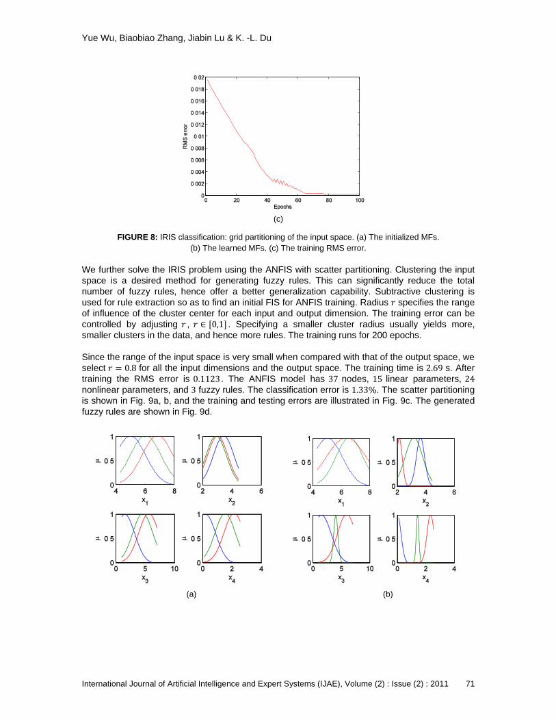
Yue Wu, Biaobiao Zhang, Jiabin Lu & K. -L. Du
International Journal of Artificial Intelligence and Expert Systems (IJAE), Volume (2) : Issue (2) : 2011 71
(c)
FIGURE 8: IRIS classification: grid partitioning of the input space. (a) The initialized MFs.
(b) The learned MFs. (c) The training RMS error.
We further solve the IRIS problem using the ANFIS with scatter partitioning. Clustering the input
space is a desired method for generating fuzzy rules. This can significantly reduce the total
number of fuzzy rules, hence offer a better generalization capability. Subtractive clustering is
used for rule extraction so as to find an initial FIS for ANFIS training. Radius 𝑟 specifies the range
of influence of the cluster center for each input and output dimension. The training error can be
controlled by adjusting 𝑟 , 𝑟 ∈ [0,1] . Specifying a smaller cluster radius usually yields more,
smaller clusters in the data, and hence more rules. The training runs for 200 epochs.
Since the range of the input space is very small when compared with that of the output space, we
select 𝑟 = 0.8 for all the input dimensions and the output space. The training time is 2.69 s. After
training the RMS error is 0.1123 . The ANFIS model has 37 nodes, 15 linear parameters, 24
nonlinear parameters, and 3 fuzzy rules. The classification error is 1.33%. The scatter partitioning
is shown in Fig. 9a, b, and the training and testing errors are illustrated in Fig. 9c. The generated
fuzzy rules are shown in Fig. 9d.
(a) (b)
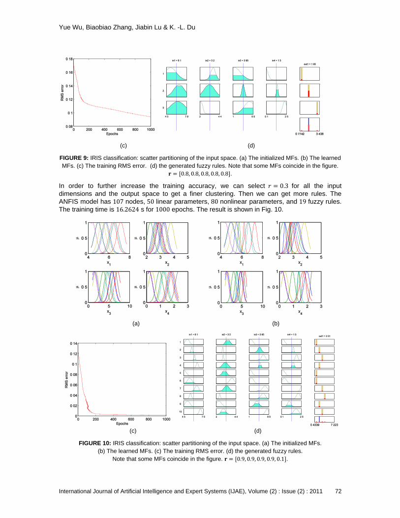
Yue Wu, Biaobiao Zhang, Jiabin Lu & K. -L. Du
International Journal of Artificial Intelligence and Expert Systems (IJAE), Volume (2) : Issue (2) : 2011 72
(c) (d)
FIGURE 9: IRIS classification: scatter partitioning of the input space. (a) The initialized MFs. (b) The learned
MFs. (c) The training RMS error. (d) the generated fuzzy rules. Note that some MFs coincide in the figure.
𝐫 = [0.8, 0.8, 0.8, 0.8, 0.8]. In order to further increase the training accuracy, we can select 𝑟 = 0.3 for all the input
dimensions and the output space to get a finer clustering. Then we can get more rules. The
ANFIS model has 107 nodes, 50 linear parameters, 80 nonlinear parameters, and 19 fuzzy rules.
The training time is 16.2624 s for 1000 epochs. The result is shown in Fig. 10.
(a) (b)
(c) (d)
FIGURE 10: IRIS classification: scatter partitioning of the input space. (a) The initialized MFs.
(b) The learned MFs. (c) The training RMS error. (d) the generated fuzzy rules.
Note that some MFs coincide in the figure. 𝐫 = [0.9, 0.9, 0.9, 0.9, 0.1].
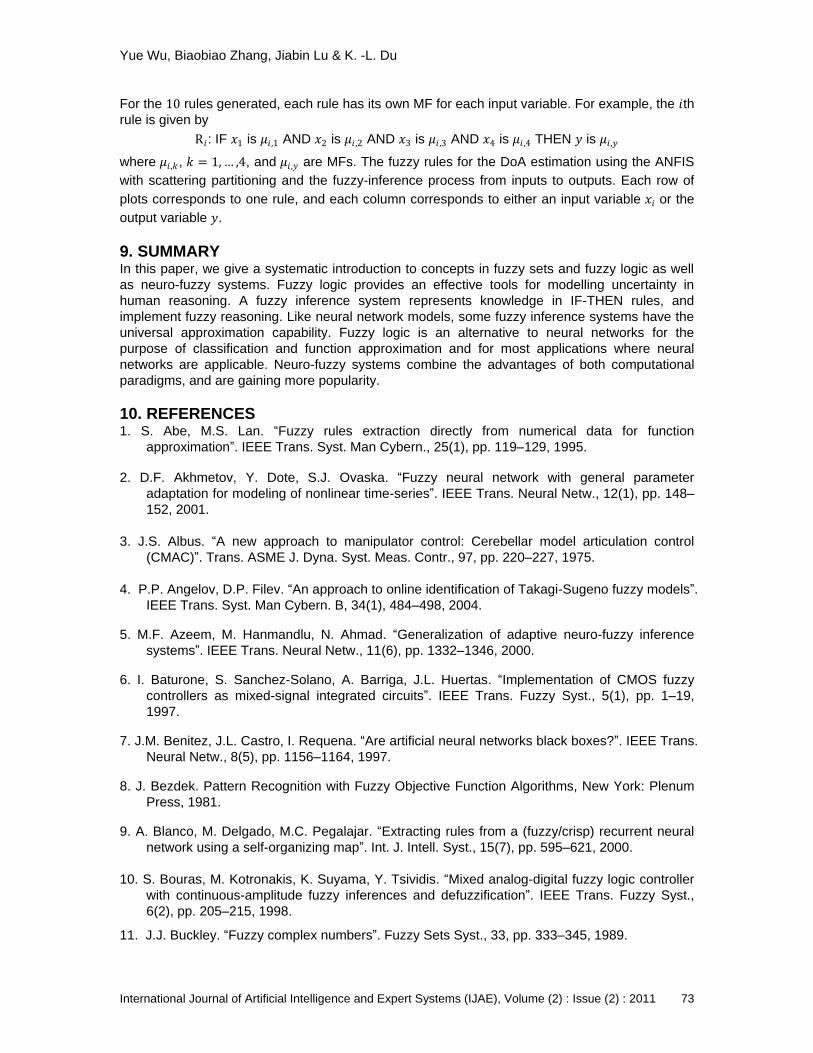
Yue Wu, Biaobiao Zhang, Jiabin Lu & K. -L. Du
International Journal of Artificial Intelligence and Expert Systems (IJAE), Volume (2) : Issue (2) : 2011 73
For the 10 rules generated, each rule has its own MF for each input variable. For example, the 𝑖th
rule is given by
R𝑖: IF 𝑥1 is 𝜇𝑖,1 AND 𝑥2 is 𝜇𝑖 ,2 AND 𝑥3 is 𝜇𝑖,3 AND 𝑥4 is 𝜇𝑖 ,4 THEN 𝑦 is 𝜇𝑖 ,𝑦
where 𝜇𝑖 ,𝑘 , 𝑘 = 1, … ,4, and 𝜇𝑖,𝑦 are MFs. The fuzzy rules for the DoA estimation using the ANFIS
with scattering partitioning and the fuzzy-inference process from inputs to outputs. Each row of
plots corresponds to one rule, and each column corresponds to either an input variable 𝑥𝑖 or the
output variable 𝑦.
9. SUMMARY In this paper, we give a systematic introduction to concepts in fuzzy sets and fuzzy logic as well
as neuro-fuzzy systems. Fuzzy logic provides an effective tools for modelling uncertainty in
human reasoning. A fuzzy inference system represents knowledge in IF-THEN rules, and
implement fuzzy reasoning. Like neural network models, some fuzzy inference systems have the
universal approximation capability. Fuzzy logic is an alternative to neural networks for the
purpose of classification and function approximation and for most applications where neural
networks are applicable. Neuro-fuzzy systems combine the advantages of both computational
paradigms, and are gaining more popularity.
10. REFERENCES 1. S. Abe, M.S. Lan. ―Fuzzy rules extraction directly from numerical data for function
approximation‖. IEEE Trans. Syst. Man Cybern., 25(1), pp. 119–129, 1995.
2. D.F. Akhmetov, Y. Dote, S.J. Ovaska. ―Fuzzy neural network with general parameter
adaptation for modeling of nonlinear time-series‖. IEEE Trans. Neural Netw., 12(1), pp. 148–
152, 2001.
3. J.S. Albus. ―A new approach to manipulator control: Cerebellar model articulation control
(CMAC)‖. Trans. ASME J. Dyna. Syst. Meas. Contr., 97, pp. 220–227, 1975.
4. P.P. Angelov, D.P. Filev. ―An approach to online identification of Takagi-Sugeno fuzzy models‖.
IEEE Trans. Syst. Man Cybern. B, 34(1), 484–498, 2004. 5. M.F. Azeem, M. Hanmandlu, N. Ahmad. ―Generalization of adaptive neuro-fuzzy inference
systems‖. IEEE Trans. Neural Netw., 11(6), pp. 1332–1346, 2000. 6. I. Baturone, S. Sanchez-Solano, A. Barriga, J.L. Huertas. ―Implementation of CMOS fuzzy
controllers as mixed-signal integrated circuits‖. IEEE Trans. Fuzzy Syst., 5(1), pp. 1–19,
1997. 7. J.M. Benitez, J.L. Castro, I. Requena. ―Are artificial neural networks black boxes?‖. IEEE Trans.
Neural Netw., 8(5), pp. 1156–1164, 1997. 8. J. Bezdek. Pattern Recognition with Fuzzy Objective Function Algorithms, New York: Plenum
Press, 1981. 9. A. Blanco, M. Delgado, M.C. Pegalajar. ―Extracting rules from a (fuzzy/crisp) recurrent neural
network using a self-organizing map‖. Int. J. Intell. Syst., 15(7), pp. 595–621, 2000.
10. S. Bouras, M. Kotronakis, K. Suyama, Y. Tsividis. ―Mixed analog-digital fuzzy logic controller
with continuous-amplitude fuzzy inferences and defuzzification‖. IEEE Trans. Fuzzy Syst.,
6(2), pp. 205–215, 1998. 11. J.J. Buckley. ―Fuzzy complex numbers‖. Fuzzy Sets Syst., 33, pp. 333–345, 1989.
Yue Wu, Biaobiao Zhang, Jiabin Lu & K. -L. Du
International Journal of Artificial Intelligence and Expert Systems (IJAE), Volume (2) : Issue (2) : 2011 74
12. J.J. Buckley. ―Sugeno type controllers are universal controllers‖. Fuzzy Sets Syst., 53, pp.
299–304, 1993.
13. J.J. Buckley, Y. Hayashi, E. Czogala. ―On the equivalence of neural nets and fuzzy expert
systems‖. Fuzzy Sets Syst., 53, pp. 129–134, 1993.
14. J.J. Buckley, E. Eslami. An Introduction to Fuzzy Logic and Fuzzy Sets, Heidelberg: Physica-
Verlag, 2002.
15. J.L. Castro. ―Fuzzy logic controllers are universal approximators‖. IEEE Trans Syst Man
Cybern., 25(4), pp. 629–635, 1995. 16. J.L. Castro, C.J. Mantas, J. Benitez. ―Interpretation of artificial neural networks by means of
fuzzy rules‖. IEEE Trans. Neural Netw., 13(1), pp. 101–116, 2002. 17. A. Cechin, U. Epperlein, B. Koppenhoefer, W. Rosenstiel. ―The extraction of Sugeno fuzzy
rules from neural networks‖, in Proc. Euro. Symp. Artif. Neural Netw., Bruges, Belgium, 1996,
pp. 49–54.
18. M.S. Chen, R.J. Liou. ―An efficient learning method of fuzzy inference system‖, in Proc. IEEE
Int. Fuzzy Syst. Conf., Seoul, Korea, 1999, pp. 634–638.
19. C.B. Cheng, E.S. Lee. ―Fuzzy regression with radial basis function network‖. Fuzzy Sets Syst.,
119, pp. 291–301, 2001.
20. S. Chiu. ―Fuzzy model identification based on cluster estimation‖. J. Intell. & Fuzzy Syst., 2(3),
pp. 267–278, 1994.
21. S.L. Chiu. ―A cluster estimation method with extension to fuzzy model identification‖, in Proc.
IEEE Int. Conf. Fuzzy Syst., Orlando, FL, 2, 1994, pp. 1240–1245. 22. K.B. Cho, B.H. Wang. ―Radial basis function based adaptive fuzzy systems and their
applications to system identification and prediction‖. Fuzzy Sets Syst., 83, pp. 325–339, 1996.
23. M.Y. Chow, S. Altrug, H.J. Trussell. ―Heuristic constraints enforcement for training of and
knowledge extraction from a fuzzy/neural architecture—Part I: Foundations‖. IEEE Trans.
Fuzzy Syst., 7(2), pp. 143–150, 1999.
24. U. Cilingiroglu, B. Pamir, Z.S. Gunay, F. Dulger. ―Sampled-analog implementation of
application-specific fuzzy controllers‖. IEEE Trans. Fuzzy Syst., 5(3), pp. 431–442, 1997.
25. A. Costa, A. De Gloria, P. Farabosch, A. Pagni, G. Rizzotto. ―Hardware solutions of fuzzy
control‖. Proc. IEEE, 83(3), pp. 422–434, 1995. 26. T. Denoeux, M.H. Masson. ―Principal component analysis of fuzzy data using autoassociative
neural networks‖. IEEE Trans. Fuzzy Syst., 12(3), pp. 336–349, 2004.
27. S. Dick. ―Toward complex fuzzy logic‖. IEEE Trans. Fuzzy Syst., 13(3), pp. 405–414, 2005.
28. J.A. Dickerson, B. Kosko. ―Fuzzy function learning with covariance ellipsoids‖, in Proc. IEEE
Int. Conf. Neural Netw., San Francisco, 3, 1993, pp. 1162–1167.
29. K.-L. Du, M.N.S. Swamy. Neural Networks in a Softcomputing Framework, London: Springer,
2006.
Yue Wu, Biaobiao Zhang, Jiabin Lu & K. -L. Du
International Journal of Artificial Intelligence and Expert Systems (IJAE), Volume (2) : Issue (2) : 2011 75
30. K.-L. Du. ―Clustering: a neural network approach‖. Neural Netw., 23(1), pp. 89–107, 2010.
31. C. Dualibe, M. Verleysen, P.G.A. Jespers. Design of Analog Fuzzy Logic Controllers in
CMOS Technology, Netherlands: Kluwer, 2003.
32. W. Duch. ―Uncertainty of data, fuzzy membership functions, and multilayer perceptrons‖.
IEEE Trans. Neural Netw., 16(1), pp. 10–23, 2005.
33. M.J. Er, S. Wu. ―A fast learning algorithm for parsimonious fuzzy neural systems‖. Fuzzy Sets
Syst., 126, pp. 337–351, 2002.
34. S.E. Fahlman, C. Lebiere. ―The cascade-correlation learning architecture‖, in Advances in
Neural Information Processing Systems 2, D.S. Touretzky, Ed. San Mateo, CA: Morgan
Kaufmann, 1990, pp. 524–532.
35. G. Ferrari-Trecate, R. Rovatti. ―Fuzzy systems with overlapping Gaussian concepts:
Approximation properties in Sobolev norms‖. Fuzzy Sets Syst., 130, pp. 137–145, 2002.
36. M. Figueiredo, F. Gomides, A. Rocha, R. Yager. ―Comparison of Yager’s level set method for
fuzzy logic control with Mamdani and Larsen methods‖. IEEE Trans. Fuzzy Syst., 2, pp. 156–
159, 1993.
37. B. Gabrays, A. Bargiela. ―General fuzzy min-max neural networks for clustering and
classification‖. IEEE Trans. Neural Netw., 11(3), pp. 769–783, 2000.
38. S.I. Gallant. ―Connectionist expert systems‖. Commun. of ACM, 31(2), pp. 152–169, 1988.
39. S. Guillaume. ―Designing fuzzy inference systems from data: An interpretability-oriented
review‖. IEEE Trans. Fuzzy Syst., 9(3), pp. 426–443, 2001.
40. Y. Hayashi, J.J. Buckley, E. Czogala. ―Fuzzy neural network with fuzzy signals and weights‖.
Int. J. Intell. Syst., 8(4), pp. 527–537, 1993.
41. P. Holmblad, J. Ostergaard. ―Control of a cement kiln by fuzzy logic‖, in Fuzzy Information
and Decision Processes, M.M. Gupta, E. Sanchez, Eds. Amsterdam: North-Holland, 1982,
pp. 389–399.
42. T. Hong, C. Lee. ―Induction of fuzzy rules and membership functions from training examples‖.
Fuzzy Sets Syst., 84, pp. 33–37, 1996.
43. K.J. Hunt, R. Haas, R. Murray-Smith. ―Extending the functional equivalence of radial basis
function networks and fuzzy inference systems‖. IEEE Trans. Neural Netw., 7(3), pp. 776–
781, 1996.
44. J.F. Hurdle. ―The synthesis of compact fuzzy neural circuits‖. IEEE Trans. Fuzzy Syst., 5(1),
pp. 44–55, 1997.
45. M. Ishikawa. ―Rule extraction by successive regularization‖. Neural Netw., 13(10), pp. 1171–
1183, 2000.
46. H. Ishibuchi, R. Fujioka, H. Tanaka. ―Neural networks that learn from fuzzy IF-THEN rules‖.
IEEE Trans. Fuzzy Syst., 1, pp. 85–97, 1993.
Yue Wu, Biaobiao Zhang, Jiabin Lu & K. -L. Du
International Journal of Artificial Intelligence and Expert Systems (IJAE), Volume (2) : Issue (2) : 2011 76
47. H. Jacobsson. ―Rule extraction from recurrent neural networks: A taxonomy and review‖.
Neural Comput., 17(6), pp. 1223–1263, 2005.
48. J.S.R. Jang. ―ANFIS: Adaptive-network-based fuzzy inference systems‖. IEEE Trans, Syst,
Man Cybern., 23(3), pp. 665–685, 1993.
49. J.S.R. Jang, E. Mizutani. ―Levenberg-Marquardt method for ANFIS learning‖, in Proc. Biennial
Conf. North Amer. Fuzzy Inf. Process. Soc. (NAFIPS), Berkeley, CA, 1996, pp. 87–91.
50. J.S.R. Jang, C.I. Sun. ―Functional equivalence between radial basis function Networks and
fuzzy inference systems‖. IEEE Trans. Neural Netw., 4(1), pp. 156–159, 1993.
51. J.S.R. Jang, C.I. Sun. ―Neuro-fuzzy modeling and control‖. Proc. IEEE, 83(3), pp. 378–406,
1995.
52. Y. Jin. ―Advanced fuzzy systems design and applications‖. Heidelberg: Physica-Verlag, 2003.
53. C.F. Juang, C.T. Lin. ―An on-line self-constructing neural fuzzy inference network and its
application‖. IEEE Trans. Fuzzy Syst., 6(1), pp. 12–32, 1998.
54. J. Kim, N. Kasabov. ―HyFIS: Adaptive neuro-fuzzy inference systems and their application to
nonlinear dynamical systems‖. Neural Netw., 12, pp. 1301–1319, 1999.
55. B. Kosko. ―Fuzzy system as universal approximators‖, in Proc. IEEE Int. Conf. Fuzzy Syst.,
San Diego, CA, 1992, pp. 1153–1162.
56. B. Kosko. Fuzzy engineering. Prentice Hall, Englewood Cliffs, 1997.
57. V. Kreinovich, H.T. Nguyen, Y. Yam. ―Fuzzy systems are universal approximators for a
smooth function and its derivatives‖. Int. J. Intell. Syst., 15, pp. 565–574, 2000.
58. Y.H. Kuo, C.L. Chen. ―Generic LR fuzzy cells for fuzzy hardware synthesis‖. IEEE Trans.
Fuzzy syst., 6(2), pp. 266–285, 1998.
59. R. Langari, L. Wang, J. Yen. ―Radial basis function networks, regression weights, and the
expectation-maximization algorithm‖. IEEE Trans. Syst. Man Cybern. A, 27(5), 613–623,
1997.
60. C.W. Lee, Y.C. Shin. ―Construction of fuzzy systems using least-squares method and genetic
algorithm‖. Fuzzy Sets Syst., 137, pp. 297–323, 2003.
61. L. Lemaitre, M. Patyra, D. Mlynek. ―Analysis and design of CMOS fuzzy logic controller in
current mode‖. IEEE J. Solid-State Circ., 29(3), pp. 317–322, 1994.
62. G. Leng, G. Prasad, T.M. McGinnity. ―An on-line algorithm for creating self-organizing fuzzy
neural networks‖. Neural Netw., 17, pp. 1477–1493, 2004.
63. H.X. Li, C.L.P. Chen. ―The equivalence between fuzzy logic systems and feedforward neural
networks‖. IEEE Trans. Neural Netw., 11(2), pp. 356–365, 2000.
64. C.T. Lin, Y.C. Lu. ―A neural fuzzy system with fuzzy supervised learning‖. IEEE Trans. Syst.
Man Cybern. B, 26(5), pp. 744–763, 1996.
Yue Wu, Biaobiao Zhang, Jiabin Lu & K. -L. Du
International Journal of Artificial Intelligence and Expert Systems (IJAE), Volume (2) : Issue (2) : 2011 77
65. F.J. Lin, R.J. Wai. ―Hybrid control using recurrent fuzzy neural network for linear-induction
motor servo drive‖. IEEE Trans. Fuzzy Syst., 9(1), pp. 102–115, 2001.
66. P. Liu. ―Max-min fuzzy Hopfield neural networks and an efficient learning algorithm‖. Fuzzy
Sets Syst., 112, pp. 41–49, 2000.
67. P. Liu, H. Li. ―Efficient learning algorithms for three-layer regular feedforward fuzzy neural
networks‖. IEEE Trans. Neural Netw., 15(3), 545–558, 2004.
68. P. Liu, H. Li. ―Hierarchical TS fuzzy system and its universal approximation‖. Inf. Sci., 169, pp.
279–303, 2005.
69. E.H. Mamdani. ―Application of fuzzy algorithms for control of a simple dynamic plant‖. Proc.
IEEE, 12(1), pp. 1585–1588, 1974.
70. K.J. McGarry, J. MacIntyre. ―Knowledge extraction and insertion from radial basis function
networks‖, in IEE Colloq. Applied Stat. Pattern Recogn, Birmingham, UK, 1999, pp. 15/1–
15/6
71. S. Mitra, J. Basak. ―FRBF: A fuzzy radial basis function network‖. Neural Comput. & Appl., 10,
pp. 244–252, 2001.
72. S. Mitra, Y. Hayashi. ―Neuro-fuzzy rule generation: Survey in soft computing framework‖.
IEEE Trans. Neural Netw., 11(3), pp. 748–768, 2000.
73. E. Mizutani, J.S. Jang. ―Coactive neural fuzzy modeling‖, in Proc. IEEE Int. Conf. Neural
Netw., Perth, Australia, 1995, vol. 2, pp. 760–765.
74. D. Moses, O. Degani, H.N. Teodorescu, M. Friedman, A. Kandel. ―Linguistic coordinate
transformations for complex fuzzy sets‖, in Proc. IEEE Int. Conf. Fuzzy Syst., Seoul, Korea,
1999, 3, pp. 1340–1345.
75. D. Nauck, F. Klawonn, R. Kruse. Foundations of Neuro-fuzzy Systems. New York: Wiley,
1997. 76. D. Nauck, R. Kruse. ―A neural fuzzy controller learning by fuzzy error propagation‖, in Proc.
Worksh. North Amer. Fuzzy Inf. Process. Soc. (NAFIPS92), Puerto Vallarta, Mexico, 1992,
pp. 388–397. 77. H. Nomura, I. Hayashi, N. Wakami. ―A learning method of fuzzy inference rules by descent
method‖, in Proc. IEEE Int. Conf. Fuzzy Syst., San Diego, CA, 1992, pp. 203–210. 78. A. Nurnberger, D. Nauck, R. Kruse. ―Neuro-fuzzy control based on the NEFCON-model:
Recent developments‖. Soft Comput., 2, pp. 168–182, 1999. 79. S.K. Oh, W. Pedrycz, H.S. Park. ―Multi-layer hybrid fuzzy polynomial neural networks: A
design in the framework of computational intelligence‖. Neurocomput., 64, pp. 397–431,
2005. 80. C.W. Omlin, C.L. Giles. ―Extraction of rules from discrete-time recurrent neural networks‖.
Neural Netw., 9, pp. 41–52, 1996. 81. C.W. Omlin, K.K. Thornber, C.L. Giles. ―Fuzzy finite-state automata can be deterministically
encoded into recurrent neural networks‖. IEEE Trans. Fuzzy Syst., 6, pp. 76–89, 1998.
Yue Wu, Biaobiao Zhang, Jiabin Lu & K. -L. Du
International Journal of Artificial Intelligence and Expert Systems (IJAE), Volume (2) : Issue (2) : 2011 78
82. S.K. Pal, S. Mitra. ―Multilayer perceptron, fuzzy sets, and classification‖. IEEE Trans. Neural
Netw., 3(5), pp. 683–697, 1992.
83. M.J. Patyra, J.L. Grantner, K. Koster. ―Digital fuzzy logic controller: Design and
implementation‖. IEEE Trans. Fuzzy Syst., 4(4), pp. 439–459, 1996.
84. W. Pedrycz, A.F. Rocha. ―Fuzzy-set based models of neurons and knowledge-based
networks‖. IEEE Trans. Fuzzy Syst., 1(4), pp. 254–266, 1993.
85. G.V.S. Raju, J. Zhou, R.A. Kisner. ―Hierarchical fuzzy control‖. Int. J. Contr., 54(5), pp. 1201–
1216, 1991.
86. D. Ramot, M. Friedman, G. Langholz, A. Kandel. ―Complex fuzzy logic‖. IEEE Trans. Fuzzy
Syst., 11(4), pp. 450–461, 2003.
87. D. Ramot, R. Milo, M. Friedman, A. Kandel. ―Complex fuzzy sets‖. IEEE Trans. Fuzzy Syst.,
10(2), pp. 171–186, 2002.
88. L.M. Reyneri. ―Implementation issues of neuro-fuzzy hardware: Going toward HW/SW
codesign‖. IEEE Trans. Neural Netw., 14(1), pp. 176–194, 2003.
89. M. Riedmiller, H. Braun. ―A direct adaptive method for faster backpropagation learning: the
RPROP algorithm‖, in Proc. IEEE Int. Conf. Neural Netw., San Francisco, CA, 1993, pp.
586–591.
90. A. Rizzi, M. Panella, F.M.F. Mascioli. ―Adaptive resolution min-max classifiers‖. IEEE Trans.
Neural Netw., 13(2), pp. 402–414, 2002.
91. I. Rojas, H. Pomares, J.L. Bernier, J. Ortega et al. ―Time series analysis using normalized
PG-RBF network with regression weights‖. Neurocomput., 42, pp. 267–285, 2002.
92. I. Rojas, H. Pomares, J. Ortega, A. Prieto. ―Self-organized fuzzy system generation from
training examples‖. IEEE Trans. Fuzzy Syst., 8(1), pp. 23–36, 2000.
93. M. Russo. ―Fugenesys—A fuzzy genetic neural system for fuzzy modeling‖. IEEE Trans.
Fuzzy Syst., 6(3), pp. 373–388, 1998.
94. K. Saito, R. Nakano. ―Rule extraction from facts and neural networks‖, in Proc. Int. Neural
Netw. Conf., Paris, France, pp. 379–382. Kluwer, Dordrecht, the Netherland, 1990.
95. V. Salapura. ―A fuzzy RISC processor‖. IEEE Trans. Fuzzy Syst., 8(6), pp. 781–790, 2000.
96. M. Setnes, R. Babuska, U. Kaymak, H.R. van Nauta Remke. ―Similarity measures in fuzzy
rule base simplification‖. IEEE Trans. Syst. Man Cybern. B, 28(3), pp. 376–386, 1998.
97. P.K. Simpson. ―Fuzzy min-max neural networks–Part I. classification‖. IEEE Trans. Neural
Netw., 3, pp. 776–786, 1992.
98. P.K. Simpson. ―Fuzzy min-max neural networks–Part II: clustering‖. IEEE Trans. Fuzzy Syst.,
1(1), pp. 32–45, 1993.
99. N.A. Sisman-Yilmaz, F.N. Alpaslan, L. Jain. ―ANFIS-unfolded-in-time for multivariate time
series forecasting‖. Neurocomput., 61, pp. 139–168, 2004.
Yue Wu, Biaobiao Zhang, Jiabin Lu & K. -L. Du
International Journal of Artificial Intelligence and Expert Systems (IJAE), Volume (2) : Issue (2) : 2011 79
100. E. Soria-Olivas, J.D. Martin-Guerrero, G. Camps-Valls, A.J. Serrano-Lopez, J. Calpe-
Maravilla, L. Gomez-Chova. ―A low-complexity fuzzy activation function for artificial neural
networks‖. IEEE Trans. Neural Netw., 14(6), pp. 1576–1579, 2003.
101. C.T. Sun. ―Rule-base structure identification in an adaptive-network-based inference system‖.
IEEE Trans. Fuzzy Syst., 2(1), pp. 64–79, 1994.
102. R. Tagliaferri, A. Eleuteri, M. Meneganti, F. Barone. ―Fuzzy min-max neural networks: From
classification to regression‖. Soft Comput., 5, pp. 69–76, 2001.
103. T. Takagi, M. Sugeno. ―Fuzzy identification of systems and its applications to modelling and
control‖. IEEE Trans. Syst. Man Cybern., 15(1), pp. 116–132, 1985.
104. K. Tanaka, M. Sugeno. ―Stability analysis and design of fuzzy control systems‖. Fuzzy Sets
Syst., 45, pp. 135–150, 1992.
105. R. Thawonmas, S. Abe. ―Function approximation based on fuzzy rules extracted from
partitioned numerical data‖. IEEE Trans. Syst. Man Cybern. B, 29(4), pp. 525–534, 1999.
106. A. Tickle, R. Andrews, M. Golea, J. Diederich. ―The truth will come to light: Direction and
challenges in extracting the knowledge embedded within trained artificial neural networks‖.
IEEE Trans. Neural Netw., 9(6), pp. 1057–1068, 1998.
107. V. Tresp, J. Hollatz, S. Ahmad. ―Representing probabilistic rules with networks of Gaussian
basis functions‖. Mach. Learn., 27, pp. 173–200, 1997.
108. G. Tsekouras, H. Sarimveis, E. Kavakli, G. Bafas. ―A hierarchical fuzzy-clustering approach
to fuzzy modeling‖. Fuzzy Sets Syst., 150(2), pp. 245–266, 2004.
109. K. Uehara, M. Fujise. ―Fuzzy inference based on families of 𝛼-level sets‖. IEEE Trans. Fuzzy
Syst., 1(2), pp. 111–124, 1993.
110. A. Ultsch, R. Mantyk, G. Halmans. ―Connectionist knowledge acquisition tool: CONKAT‖, in
Artificial Intelligence Frontiers in Statistics: AI and Statistics III, : D.J. Hand, Ed. London:
Chapman & Hall, 1993, pp. 256–263.
111. P. Vuorimaa. ―Fuzzy self-organizing map‖. Fuzzy Sets Syst., 66(2), pp. 223–231, 1994.
112. D. Wang, N.S. Chaudhari. ―Binary neural network training algorithms based on linear
sequential learning‖. Int J. Neural Syst., 13(5), pp. 333–351, 2003.
113. L.X. Wang. ―Fuzzy systems are universal approximators‖, in Proc. IEEE Int. Conf. Fuzzy
Syst., San Diego, CA, 1992, pp. 1163–1170.
114. L.X. Wang. ―Analysis and design of hierarchical fuzzy systems‖. IEEE Trans. Fuzzy Syst.,
7(5), pp. 617–624, 1999.
115. L.X. Wang, J.M. Mendel. ―Generating fuzzy rules by learning from examples‖. IEEE Trans.
Syst. Man Cybern., 22(6), pp. 1414–1427, 1992.
116. L.X. Wang, J.M. Mendel. ―Fuzzy basis functions, universal approximation, and orthogonal
least-squares learning‖. IEEE Trans. Neural Netw., 3(5), pp. 807–814, 1992.
Yue Wu, Biaobiao Zhang, Jiabin Lu & K. -L. Du
International Journal of Artificial Intelligence and Expert Systems (IJAE), Volume (2) : Issue (2) : 2011 80
117. L.X. Wang, C. Wei. ―Approximation accuracy of some neuro-fuzzy approaches‖. IEEE Trans.
Fuzzy Syst., 8(4), pp. 470–478, 2000.
118. S.Wang, H. Lu. ―Fuzzy system and CMAC network with B-spline membership/basis
functions are smooth approximators‖. Soft Comput., 7, pp. 566–573, 2003.
119. P.J. Werbos. ―Backpropagation through time: what it does and how to do it‖. Proc. IEEE,
78(10), pp. 1550–1560, 1990.
120. S. Wu, M.J. Er. ―Dynamic fuzzy neural networks—A novel approach to function
approximation‖. IEEE Trans. Syst. Man Cybern. B, 30(2), pp. 358–364, 2000.
121. R. Yager, D. Filev. ―Generation of fuzzy rules by mountain clustering‖. J. Intell. Fuzzy Syst.,
2(3), pp. 209–219, 1994.
122. J. Yen. ―Fuzzy logic—A modern perspective‖. IEEE Trans. Knowl. Data Eng., 11(1), pp.
153–165, 1999.
123. L.A. Zadeh. ―Fuzzy sets‖. Inf. & Contr., 8, pp. 338–353, 1965.
124. L.A. Zadeh. ―The concept of a linguistic variable and its application to approximate
reasoning–I, II, III‖. Inf. Sci., 8, pp. 199–249, pp. 301–357, 1975; 9, pp. 43–80, 1975.
125. D. Zhang, X.L. Bai, K.Y. Cai. ―Extended neuro-fuzzy models of multilayer perceptrons‖.
Fuzzy Sets Syst., 142, pp. 221–242, 2004.