Lecture 5 Pattern Projection Techniques

Visual Perception

Lecture 5Pattern Projection Techniques

Joaquim SalviUniversitat de Girona

http://www.vibot.org/

http://www.vibot.org/

http://europa.eu.int/comm/education/programmes/mundus/index_en.html

http://europa.eu.int/comm/education/programmes/mundus/index_en.html

2

Lecture 5: Pattern Projection Techniques

Contents

5. Pattern Projection Techniques5.1 Passive vs active stereo

5.2 Coded structured light

5.3 Classification: Time multiplexing

5.4 Classification: Spatial codification

5.5 Classification: Direct codification

5.6 Optimising De Bruijn patterns

5.7 Implementation of a De Bruijn pattern

3









Contents

4


INTERPRETATIONKNOWLEDGE

BASEDATABASE

InterpretationLevel

SCENEDESCRIPTIONFUSION TRACKING

SHAPEIDENTIFICATION

LOCALIZATIONSCENE

ANALYSIS

SEGMENTATION

SHAPEACQUISITION

FEATUREEXTRACTION

MOVEMENTDETECTION

TEXTUREANALYSIS

IMAGERESTORATION

EDGERESTORATION

DescriptionLevel

Image ProcessingHigh Level

FILTERINGEDGE

THINNING

EDGEDETECTION

COLOURCOMPENSATION

THRESHOLDING

GRADIENTS

RE-HISTOGRAMATION

A/D

COLOURSEPARATION

SENSOR

Image AcquisitionLevel

Image ProcessingLow Level

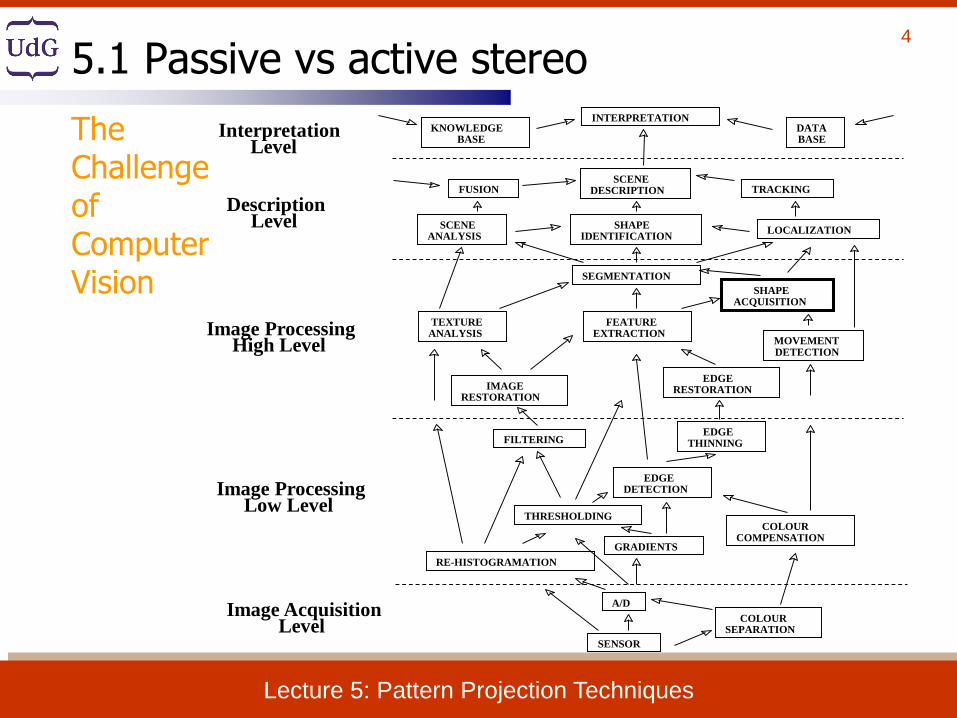
5.1 Passive vs active stereo

TheChallengeofComputer Vision

5


Shape acquisition techniques

Contact

Non-destructive Destructive

Jointed armsSlicing

Non-contact

Reflective Transmissive

Non-optical

Optical

...

Microwave radar Sonar

Passive

Active

Stereo Shading Silhouettes TextureMotion

Shape from X Interferometry

(Coded) Structured

light

Moire Holography

Source: Brian Curless


ShapeAcquisitionTechniques

6


• Correspondence problem

• geometric constraints

search along epipolar lines

• 3D reconstruction of matched pairs by triangulation


Passive Stereo

7


Arrange correspondence points

• Ordered Projections

• Projections bad order

Occlusions

• Points without homologue

ee’

I’

CC’

pq

p’ q’

QP

l l’

I

3D Object

Inverse order

ee’

I

CC’

pq

p’ q’l l’

P

Q

I’

3D Objects

Direct order

ee’

I’

I

CC’

p ?q

p’ q’l l’

P

Q

3D Object

Surface occlusion Point without homologue


Passive Stereo

8


Y

Z

X

I

M

f

m

I’

m’

X’

Y’

Z’

f’

OO’

CC’

Zw

Xw

Yw

Captured Image Captured Image

• We need at least two cameras.

• A 3D object point has three

unknown co-ordinates.

• Each 2D image point gives two

equations.

• Only a single component of the

second point is needed.


Passive Stereo

9


• One of the cameras is replaced by a light emitter

• Correspondence problem is solved by searching the pattern in the camera image (pattern decoding)


Active Stereo

10









Contents

11









Contents

12



• The correspondence problem is reduced :

• The matching between the projected pattern and the captured

one can be uniquely solved codifying the pattern.

– Stripe patterns :

• No scanning.

• Correspondence problem among

slits.

– Grid, multiple dots :

• No scanning.

• Correspondence problem among

all the imaged features (points, dots,

segments,…).

– Single dot :

• No correspondence problem.

• Scanning both axis.

– Single slit :

• No correspondence problem.

• Scanning the axis orthogonal

to the slit.

13


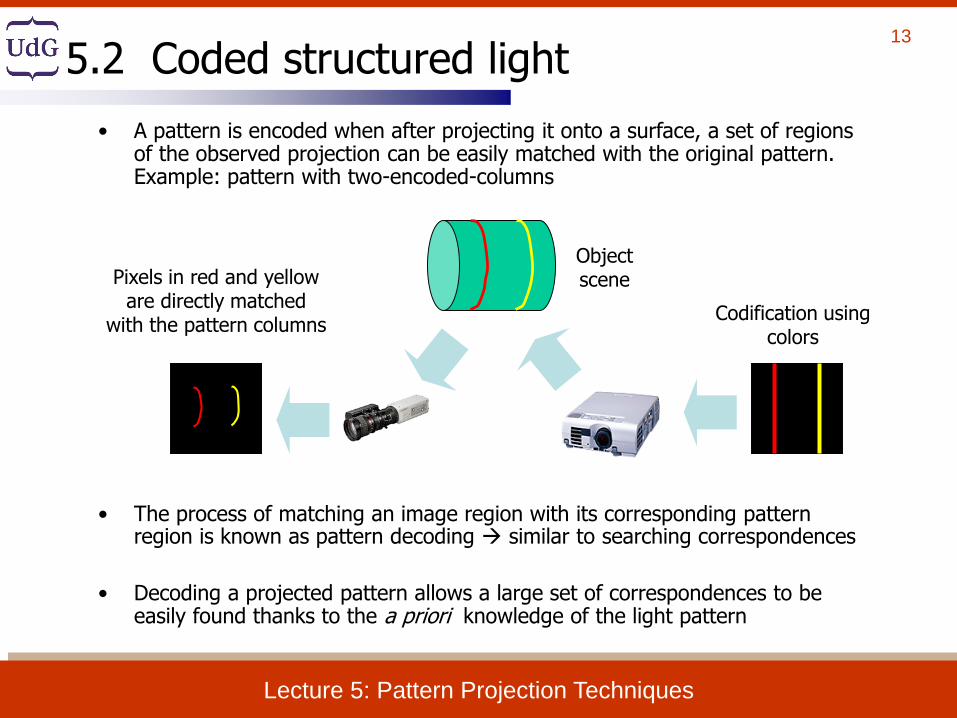
• A pattern is encoded when after projecting it onto a surface, a set of regions of the observed projection can be easily matched with the original pattern. Example: pattern with two-encoded-columns

• The process of matching an image region with its corresponding pattern region is known as pattern decoding similar to searching correspondences

• Decoding a projected pattern allows a large set of correspondences to be easily found thanks to the a priori knowledge of the light pattern

Pixels in red and yellow are directly matched

with the pattern columnsCodification using

colors

Object scene


14


• Two ways of encoding the correspondences: single axis and two axes codification it determines how the triangulation is calculated

• Decoding the pattern means locating points in the camera image whose corresponding point in the projector pattern is a priori known

Two-axes encoding

Triangulation by line-to-plane intersection

Triangulation by line-to-line intersection

Single-axis encoding

Encoded Axis


15


AXIS CODIFICATION

• Single Axis

- Row-coded patterns

- Column-coded patterns

• Both Axes

• Static Scenes- Projection of a set of patterns.

• Moving Scenes- Projection of a unique pattern.

SCENE APPLICABILITY

CODING STRATEGY

• Periodical - The codification of the tokens

is repeated periodically.

• Absolute- Each token is uniquely encoded

• Binary

• Grey Levels

• Colour

PIXEL DEPTH


16


Binary codes

Posdamer et al., Inokuchi et al., Minou et al., Trobina, Valkenburg

and McIvor, Skocaj and Leonardis, Rocchin et al., …

n-ary codes Caspi et al., Horn and Kiryati,

Osawa et al.,…

Gray code + Phase shifting

Bergmann, Sansoni et al., Wiora, Gühring, …

TIME-MULTIPLEXING

Hybrid methods K. Sato, Hall-Holt and

Rusinkiewicz, Wang et al., …

Non-formal codification

Maruyama and Abe, Durdle et al., Ito and Ishii, Boyer and Kak, Chen

et al., …

De Bruijn sequences Hügli and Maître, Monks et al.,

Vuylsteke and Oosterlinck, Salvi et al. Lavoi et al., Zhang et al., …

SPATIAL CODIFICATION

M-arrays

Morita et al., Petriu et al., Kiyasu et al., Spoelder et al., Griffin and

Yee, Davies and Nixon, Morano et al., …

Grey levels Carrihill and Hummel, Chazan and

Kiryati, Hung, ... DIRECT CODIFICATION Colour

Tajima and Iwakawa, Smutny and Pajdla, Geng, Wust and Capson, T.

Sato, …


17









Contents

18









Contents

19


TIME-MULTIPLEXING

Binary codes




Osawa et al.,…








et al., …



M-arrays



DIRECT CODIFICATION


Kiryati, Hung, ...

Colour Tajima and Iwakawa, Smutny and Pajdla, Geng, Wust and Capson, T.

Sato, …


20


• The time-multiplexing paradigm consists in projecting a series of light patterns so that every encoded point is identified with the sequence of intensities that receives

• The most common structure of the patterns is a sequence of stripes increasing its length by the time

single-axis encoding

• Advantages:

– high resolution a lot of 3D points

– High accuracy (order of m)

– Robustness against colorful objects (using binary patterns)

• Drawbacks:

– Static objects only

– Large number of patterns High

computing timePattern 1

Pattern 2

Pattern 3

Projected over time

Example: 3 binary-encoded patterns which allows the measuring

surface to be divided in 8 sub-regions

5.3 Time multiplexing

21


5.3 Time-multiplexing: Binary codes (I)

Pattern 1

Pattern 2

Pattern 3

Projected over time

• Every encoded point is identified by the sequence of intensities that receives

• n patterns must be projected in order to encode 2n stripes

Example: 7 binary patterns proposed by Posdamer & Altschuler

…

Codeword of this píxel: 1010010 identifies

the corresponding pattern stripe

22


Posdamer et al.

Inokuchi et al.

Minou et al.

Trobina

Valkenburg and McIvor

Skocaj and Leonardis

Binary codes

Rocchini et al.

Static

Scene applicability Moving

Binary

Grey levels

Pixel depth

Colour

Periodical Coding strategy

Absolute

• Coding redundancy: every edge between adjacent stripes can be decoded by the sequence at its left or at its right

5.3 Time-multiplexing: Binary codes (II)

23


Using a 4-ary code, 3 patterns are used to encode 64 stripes

(Horn & Kiryati)

• n-ary codes reduce the number of patterns by increasing the number of projected intensities (grey levels/colours) increases the basis of the code

• The number of patterns, the number of grey levels or colours and the number of encoded stripes are strongly related fixing two of these parameters the reamaining one is obtained

Using a binary code, 6 patterns are necessary to encode 64 stripes

5.3 Time-multiplexing: N-ary codes (I)

24


Caspi et al. √ √ √

Horn and Kiryati √ √ √ N-ary codes

Osawa et al. √ √ √

Static


Binary

Grey levels

Pixel depth

Colour


Absolute

• n-ary codes reduce the number of patterns by increasing the number of projected intensities (grey levels/colours)

5.3 Time-multiplexing: N-ary codes (II)

25


5.3 Time-multiplexing: Gray code+Phase shifting (I)

Gühring’s line-shift technique

• A sequence of binary patterns (Gray encoded) are projected in order to divide the object in regions

• An additional periodical pattern is projected

• The periodical pattern is projected several times by shifting it in one direction in order to increase the resolution of the system similar to a

laser scanner

Example: three binary patterns

divide the object in 8 regions

Without the binary patterns we would

not be able to distinguish among all the projected

slits

Every slit always falls in the same

region

26


Bergmann

Sansoni et al.

Wiora

Gray Code + Phase Shift

Gühring

Static


Binary

Grey levels

Pixel depth

Colour


Absolute

• A periodical pattern is shifted and projected several times in order to increase the resolution of the measurements

• The Gray encoded patterns permit to differentiate among all the periods of the shifted pattern

5.3 Time-multiplexing: Gray code+Phase shifting (II)

27


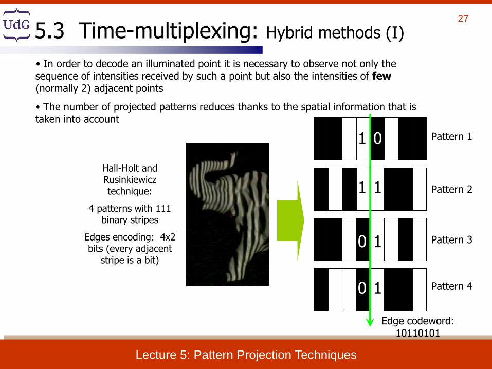
• In order to decode an illuminated point it is necessary to observe not only the sequence of intensities received by such a point but also the intensities of few(normally 2) adjacent points

• The number of projected patterns reduces thanks to the spatial information that is taken into account

Hall-Holt and Rusinkiewicz technique:

4 patterns with 111 binary stripes

Edges encoding: 4x2 bits (every adjacent

stripe is a bit)

1

1

1

1

1

0

0

0 Pattern 1

Pattern 2

Pattern 3

Pattern 4

Edge codeword: 10110101

5.3 Time-multiplexing: Hybrid methods (I)

28


K. Sato

Hall-Holt and Rusinkiewicz Hybrid methods

Wang et al.

Static


Binary

Grey levels

Pixel depth

Colour


Absolute

5.3 Time-multiplexing: Hybrid methods (II)

29


Spatialcodification

De Bruijn (64 slits) Salvi (29x29 slits) Morano (45x45 dot array)

Time-multiplexing

Posdamer (128 stripes) Horn (64 stripes) Gühring (113 slits)

Gühring

5.3 Time-multiplexing: Results

30


Types of techniques

Time-multiplexing

• Highest resolution

• High accuracy

• Easy implementation

• Large number of patterns

• Only motionless objects

Spatial codification

• A unique pattern is required

• Can measure moving objects

• Lower resolution than time-multiplexing

• More complex decoding stage

• Occlusions problem

Direct codification• High resolution

• Few patterns

• Very sensitive to image noise

cameras with large depth-per-pixel required

• Sensitive to limited bandwith of LCD projectors special projector

devices are usually required


5.3 Time-multiplexing: Conclusions

31









Contents

32









Contents

33


TIME-MULTIPLEXING

Binary codes




Osawa et al.,…








et al., …



M-arrays



DIRECT CODIFICATION


Kiryati, Hung, ...


Sato, …

5.4 Spatial Codification

34


• Spatial codification paradigm encodes a set of points with the information contained in a neighborhood (called window) around them

• The codification is condensed in a unique pattern instead of multiplexing it along time

• The size of the neighborhood (window size) is proportional to the number of encoded points and inversely proportional to the number of used colors

• The aim of these techniques is to obtain a one-shot measurement system moving objects can be measured

• Advantages:

• Moving objects supported

• Possibility to condense the codification into a unique pattern

• Drawbacks:

• Discontinuities on the object surface can produce erroneous window decoding (occlusions problem)

• The higher the number of used colours, the more difficult to correctly identify them when measuring non-neutral coloured surfaces

5.4 Spatial Codification

35


• The first group of techniques that appeared used codification schemes with no mathematical formulation.

• Drawbacks:

- the codification is not optimal and often produces ambiguities since different regions of the pattern are identical

-the structure of the pattern is too complex for a good image processing

Maruyama and Abe

complex structure based on slits

containing random cuts

Durdle et al. periodic pattern

5.4 Spatial Codification: Non-formal codification (I)

36


Maruyama and Abe

Durdle et al.

Ito and Ishii

Boyer and Kak


Chen et al.

Static


Binary

Grey levels

Pixel depth

Colour


Absolute

5.4 Spatial Codification: Non-formal codification (II)

37


• Formulation:

Given P={1,2,...,p} set of colours.

• We want to determine S={s1,s2,...sn} sequence of coloured slits.

Node: {ijk}

Number of nodes: p3 nodes.

Transition {ijk} {rst} j = r, k = s

• The problem is reduced to obtain the path which visits all the nodes of the

graph only once (a simple variation of the Salesman’s problem).

– Backtracking based solution.

– Deterministic and optimally solved by Griffin.

• A De Bruijn sequence (or pseudorrandom sequence) of order m over an alphabet of nsymbols is a circular string of length nm that contains every substring of length m exactly once (in this case the windows are unidimensional).

1000010111101001m=4 (window size)

n=2 (alphabet symbols)

m = 3 (window size)

n = p (alphabet symbols)

3

pVR

5.4 Spatial Codification: De Bruijn sequences (I)

38


Path: (111),(112),(122),(222),(221),(212),(121),(211).

Slit colour sequence:111,2,2,2,1,2,1,1 Maximum 10 slits.

‘1’ Red

‘2’ Green

111

112

121

212

122

211

221

222

m = 3

n = 282

2

33

2

pVR

p

Example:

5.4 Spatial Codification: De Bruijn sequences (II)

39


• The De Bruijn sequences are used to define coloured slit patterns (single axis codification) or grid patterns (double axis codification)

• In order to decode a certain slit it is only necessary to identify one of the windows in which it belongs to

Zhang et al.: 125 slits encoded with a De Bruijn sequence of 5 colors and window size of 3 slits

Salvi et al.: grid of 2929 where a De Bruijn sequence of 3 colors and window size of 3 slits is used to encode the vertical and horizontal

slits

5.4 Spatial Codification: De Bruijn sequences (III)

40


Hügli and Maître

Monks et al.

Salvi et al.

Lavoie et al.

De Bruijn sequences

Zhang et al.

Static


Binary

Grey levels

Pixel depth

Colour


Absolute

5.4 Spatial Codification: De Bruijn sequences (IV)

41


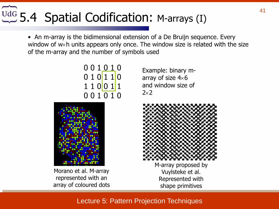
• An m-array is the bidimensional extension of a De Bruijn sequence. Every window of wh units appears only once. The window size is related with the size of the m-array and the number of symbols used

0 0 1 0 1 00 1 0 1 1 01 1 0 0 1 10 0 1 0 1 0

Morano et al. M-array represented with an

array of coloured dots

Example: binary m-array of size 46 and window size of 22

M-array proposed by Vuylsteke et al.

Represented with shape primitives

5.4 Spatial Codification: M-arrays (I)

42


Morita et al.

Petriu et al.

Vuylsteke and Oosterlinck

Kiyasu et al.

Spoelder et al.

Griffin and Yee

Davies and Nixon

M-arrays

Morano et al.

Static


Binary

Grey levels

Pixel depth

Colour


Absolute

5.4 Spatial Codification: M-arrays (II)

43


Time-multiplexing




GühringDe Bruijn

5.4 Spatial Codification: Results

44


Types of techniques

Time-multiplexing


• High accuracy











• Few patterns






5.4 Spatial Codification: Results

45









Contents

46









Contents

47


TIME-MULTIPLEXING

Binary codes




Osawa et al.,…








et al., …



M-arrays



DIRECT CODIFICATION


Kiryati, Hung, ...


Sato, …

5.5 Direct Codification

48


• Every encoded pixel is identified by its own intensity/colour

• Since the codification is usually condensed in a unique pattern, the spectrum of intensities/colours used is very large

• Additional reference patterns must be projected in order to differentiate among all the projected intensities/colours:

• Ambient lighting (black pattern)

• Full illuminated (white pattern)

• …

• Advantages:

– Reduced number of patterns

– High resolution can be teorically achieved (all points are coded)

• Drawbacks:

– Very noisy in front of reflective properties of the objects, non-linearities in the camera spectral response and projector spectrum non-standard

light emitters are required in order to project single wave-lengths

– Low accuracy (order of 1 mm)

5.5 Direct Codification

49


• Every encoded point of the pattern is identified by its intensity level

Carrihill and Hummel Intensity Ratio Sensor: fade

from black to white

Requirements to obtain high resolution

Every slit is identified by its own intensity

• Every slit must be projected using a single wave-length

• Cameras with large depth-per-pixel (about 11 bits) must be used in order to differentiate all the projected intensities

5.5 Direct Codification: Grey levels (I)

50


Carrihill and Hummel

Chazan and Kiryati Grey levels

Hung

Static


Binary

Grey levels

Pixel depth

Colour


Absolute

5.5 Direct Codification: Grey levels (II)

51


• Every encoded point of the pattern is identified by its colour

Tajima and Iwakawa rainbow

pattern

(the rainbow is generated with a

source of white light passing through a

crystal prism)

T. Sato patterns capable of cancelling the object colour by projecting three shifted

patterns

(it can be implemented with an LCD projector if few colours are

projected drawback: the

pattern becomes periodic in order to maintain a good

resolution)

5.5 Direct Codification: Colour (I)

52


Tajima and Iwakawa

Smutny and Pajdla

Geng

Wust and Capson

Colour

T. Sato

Static


Binary

Grey levels

Pixel depth

Colour


Absolute

5.5 Direct Codification: Colour (II)

53

Lecture 5: Pattern Projection TechniquesLecture 5: Pattern Projection Techniques

Time-multiplexing




Direct codification

Sato (64 slits)

5.5 Direct Codification: Results

54


Types of techniques

Time-multiplexing


• High accuracy











• Few patterns






5.5 Direct Codification: Conclusions

55









Contents

56









Contents

57


Guidelines

Requirements Best technique

• High accuracy


• Static objects

• No matter the number of patterns

Phase shift + Gray code

Gühring’s line-shift technique

• High accuracy

• High resolution

• Static objects

• Minimum number of patterns

N-ary pattern Horn & Kiryati

Caspi et al.

• High accuracy

• Good resolution

• Moving objects

Optimised Bruijn pattern

Salvi and Pagés.

58


Presentation outline

2.- An Optimised one-shot technique

– Typical one-shot patterns

– Optimal pattern

– A new coding strategy

– Implementation design

– Experimental results

– Conclusions

59


Typical one-shot patterns

Stripe pattern Grid pattern

De Bruijn codification

M-array codification

Array of dotsArray of shape

primitives

Multi-slit pattern

Checkerboard pattern

Image by Li Zhang

60


Best one-shot patterns

De Bruijn patterns

Stripe patterns

High resolution and good accuracy

Multi-slit patterns

High accuracy and good resolution

Grid patterns Low resolution

M-array patterns

Array of dotsLow resolution and inaccurate sub-pixel localisation of the dots

Shape primitives

Low accuracy and difficult sub-pixel localisation of shape primitives

Checkerboard Low resolution

61


Optimising De Bruijn patterns: interesting features

Optimisation Advantages

Maximising resolutionLarger number of correspondences in a single shot

Maximising accuracy Better quality in the 3D reconstruction

Minimising the window size

More robustness against discontinuities in the object surface

Minimising the number of colours

More robustness against non-neutral coloured objects and noise

62


Optimisation: maximising resolution

Stripe patterns: achieve maximum resolution since they are formed by adjacent bands of pixels.

Multi-slit patterns: the maximum resolution is not achieved since black gaps are introduced between the slits

Ideal pattern: the one which downsamples the projector resolution so that all the projected pixels are perceived in the camera image in fact only columns or rows must be identified

in order to triangulate 3D points.

63


Optimisation: maximising accuracy

Ideal pattern: multi-slit patterns allow intensity peaks to be detected with precise sub-pixel accuracy

Multi-slit pattern Stripe pattern

Edge detection between stripes: need to find edges in the three RGB channels

the location of the edges does not coincide

Figure by Jens Gühring

RGB channels intensity profile of a row of the

image

64


Optimisation: minimising the window size and the number of colours

Maximising Minimising

Number of

colours

• Larger resolution

• Smaller distance in the Hue space more difficult colour

identification

• Smaller resolution

• Larger distance in the Hue space Easier colour

identification

Window size

• Larger resolution

• Danger to violate the local smoothness assumption

• Smaller resolution

• More robustness against surface discontinuities

If both the number of colours and the window size are minimised the resolution decreases

65


Optimising De Bruijn patterns: summary

Optimisation Best pattern

Maximising resolution Stripe pattern

Maximising accuracy Multi-slit pattern

Minimising the window size and the number of

colours preserving a good resolution

Stripe pattern + multi-slit pattern

66


A new hybrid pattern

inte

ns

ity

Horizontal scanline

Combination of the advantages of stripe patterns

and multi-slit patterns

Stripe pattern in the RGB space

Multi-slit pattern in the Luminance channel

inte

ns

ity

Horizontal scanline

inte

ns

ity

Horizontal

scanline

Projected luminance profile

Perceived luminance profile

67


The new coding strategy

Given n different values of Hue and a window

size of length m

A pattern with 2nm stripes is defined with a square Luminance profile with alternating full-illuminated and half-

illuminated stripes

The pattern is divided in n periods so that all the full-illuminated stripes of every period share the same Hue

The half-illuminated stripes of every period are coloured according to a De Bruijn sequence of order m-1

and the same n Hue values

Example: n=4, m=3

128 stripes

32 stripes32 stripes

16 coded stripes 16 coded stripes…

…

68


The new coding strategy

S={0010203112132233}0=red; 1=green; 2=cyan; 3=blue

69


Implementation design of the coded structured light technique

Colour

selection and

calibration

Colours

AM, Am

Geometric

calibration

K1, Pc, Pp

RGB channel

alignment

calibration

gHr, gHb

Peak

compensation

calibration

offsets

RGB

alignment

Image

rectification

Peak

detection

Peak

decoding

Peak

compensation

Colour

rectification

3D

reconstruction

Offline

processes

Online

processes

Radial

distortion

removal

Most of the processes of this schema are valid for any one-shot technique

based on colour structured light

http://www.itcompany.com/images/computer.gif




70


Offline processing: RGB channel misalignment calibration

The grid cross-points coordinates are located with sub-pixel accuracy in each RGB channel.

Two homographies gHr and gHb are calculated in order to reduce the misalignment between the red and the blue channel with respect to the green.

RGB image

red channel

green channel

blue channel

red grid

green grid

blue grid

It should be

a white grid

Homographies

71


Offiline processing: geometric calibration

- Camera: Pinhole + Radial lens distortion

- Projector: like a reverse camera

72


Offline processing: colour selection (I)

Example:

selection of

n=3 coloursHue

1) Select n

equi-spaced

Hue levels

2) Project the n Hue values with different Luminance values and

interpolate their response curve.

Each RGB channel has different sensitivity the intensity perceived is

in function of the projected Hue

3) Given the maximum and

minimum levels of luminances that

we want to perceive the

corresponding projecting

luminances for every Hue can be

chosedemitted Luminancep

erc

eiv

ed

Lu

min

an

ce

73


Offline processing: colour selection (II)

The projector-camera system introduces a strong colour

cross-talk which makes colour identification difficult.

The cross-talk can be reduced with a calibration procedure:

• a pure red, green and blue patterns are projected over a colour-

neutral panel.

• a linear mapping is calculated between the colour instructions

and the perceived ones a cross-talk matrix is obtained

• this matrix approximates the behaviour of the projector-camera

system This matrix will be used online to reduce the cross-talk.

The highest cross-talk exists between the green and the red channel

74


Offline processing: peak compensation calibration

Every peak of luminosity is affected by the colours of the surrounding

stripes the detected peak position is affected by an offset

Peak compensation calibration: the pattern containing both full and half-

illuminated stripes is projected and then the pattern only containing the

full-illuminated stripes is also projected

Maxima peak

sub-pixel position-

offsetsThe same process is made

with the minima peaks

Maxima peak

sub-pixel position

75


Online processing

Colours

AM, AmK1, Pc, Pp

gHr, gHb offsets

RGB

alignment

Image

rectification

Peak

detection

Peak

decoding

Peak

compensation

Colour

rectification

3D

reconstructionOnline

processes

Radial

distortion

removal

Stripes location: binarised 2nd

derivative of the luminance channel

Radial

distortion

removal

RGB

alignment

Image

rectification

Peak

detection

Peak

decoding

Colour

rectification

Peak decoding

1 number of period

De Bruijn: 00102031121322330

Position of the stripe inside the period

Sub-pixel location of each positive and negative

luminance peak: Blais and Rioux detector

Colour rectification by using the inverse

of the calibrated cross-talk matrix

Peak

compensation

3D

reconstruction



76


Experimental results (I)

77


Experimental results (II)

78


Conclusions

• A new coding strategy for one-shot patterns has been

presented.

• The new pattern combines the high resolution of stripe-

patterns and the high accuracy of multi-slit patterns.

• A pattern with 2nm stripes is achieved with only n levels of Hue

and a window property equal to m. (ex. 2*43 = 128 stripes)

• Given the same parameters, stripe-patterns encoded with

classical De Bruijn sequences have a resolution of nm (ex.

43 = 64 stripes)

• The resolution has been doubled.

• The pattern has a sinusoidal profile in the luminance channel

so that maximum and minimum peaks can be accurately

detected with classical peak detectors.n = Number of colours (4),

m = Window size (3)

79


Published Material

Journals– J. Pagés, J. Salvi, J. Forest. Optimised De Bruijn patterns for one-shot shape

acquisition. Image and Vision Computing. 23(8), pp 707-720, August 2005.

– J. Salvi, J. Pagés, J. Batlle. Pattern Codification Strategies in Structured Light Systems. Pattern Recognition 37(4), pp 827-849, April 2004.

– J. Batlle, E. Mouaddib and J. Salvi. A Survey: Recent Progress in Coded Structured Light as a Technique to Solve the Correspondence Problem. Pattern Recogniton 31(7), pp 963-982, July 1998.

– J. Salvi, J. Batlle and E. Mouaddib. A Robust-Coded Pattern Projection for Dynamic 3D Scene Measurement. Pattern Recognition Letters 19, pp 1055-1065, September 1998.

Recent Conferences– J. Pagès, J. Salvi and J. Forest. Optimised De Bruijn Patterns for One-Shot Shape

Acquisition. IEEE Int. Conf. on Pattern Recognition, ICPR 2004, Cambridge, Great Britain, 2004.

– J. Pagès, J. Salvi and C. Matabosch. Implementation of a robust coded structured light technique for dynamic 3D measurements. IEEE Int. Conf. on Image Processing, ICIP 2003, Barcelona, Spain, Septembre 2003.

– J. Pagès, J. Salvi, R. García and C. Matabosch. Overview of coded light projection techniques for automatic 3D profiling. IEEE Int. Conf. on Robotics and Automation, ICRA 2003, Taipei, Taiwan, May 2003.

More Information: http://eia.udg.es/~qsalvi/

Education

Lecture 5 Pattern Projection Techniques