Embed Size (px)
Citation preview

Statistical InferenceWeek 3: Hypothesis Testing and t-tests

Central Limit Theorem What is the mean height (𝜇) of all primary school children in Singapore?
Sample = Anderson Primary
Population = All primary school children in SG
Sample = DamaiPrimary
Sample = Red Swastika Primary
Sample = Zhenghua Primary
𝒙𝑨𝒏𝒅𝒆𝒓𝒔𝒐𝒏 𝑷𝒓𝒊𝒎𝒂𝒓𝒚 = Mean height of
100 children from Anderson Primary
𝒙𝑫𝒂𝒎𝒂𝒊 𝑷𝒓𝒊𝒎𝒂𝒓𝒚 = Mean height of 100
children from Damai Primary
𝒙𝑹𝒆𝒅 𝑺𝒘𝒂𝒔𝒕𝒊𝒌𝒂 = Mean height of 100 children from Red Swastika Primary
𝒙𝒁𝒉𝒆𝒏𝒈𝒉𝒖𝒂 𝑷𝒓𝒊𝒎𝒂𝒓𝒚= Mean height of 100
children from Zhenghua Primary
𝐷𝑖𝑠𝑡𝑟𝑖𝑏𝑢𝑡𝑖𝑜𝑛 𝑜𝑓 𝑚𝑒𝑎𝑛 ℎ𝑒𝑖𝑔ℎ𝑡 ~ 𝑁(𝑚𝑒𝑎𝑛 = 𝜇, 𝑠𝑡𝑎𝑛𝑑𝑎𝑟𝑑 𝑒𝑟𝑟𝑜𝑟 =𝜎
100)
…
…
…
From the sampling distribution: Mean( 𝑥) ≈ 𝜇 SD( 𝑥) < 𝜎
− As sample size increases, SD decreases

Central Limit Theorem (CLT)
The distribution of sample statistics (e.g., mean) is approximately normal, regardless of the underlying distribution, with mean =
𝜇 and variance = 𝜎2
𝑁
𝒙 ~ 𝑵(𝒎𝒆𝒂𝒏 = 𝝁, 𝒔𝒕𝒂𝒏𝒅𝒂𝒓𝒅 𝒆𝒓𝒓𝒐𝒓 =𝝈
𝒏)
Further experimentation: http://bitly.com/clt_mean
Distribution is normal
Sample mean = population mean
Sample sd = population sd divided by square root
of sample size
Applet source: Mine Çetinkaya-Rundel, Duke University

Conditions for CLT
Independence: Sampled observations must be independent:−Random sample/assignment
− If sampling without replacement, n < 10% of population
Sample Size/Skew:−Population should be normal
− If not, sample size should be large (rule of thumb: n > 30)

Confidence Interval
An interval estimate of a population parameter−Computed as sample mean +/- a
margin of error
𝑥 ± 𝑧 × 𝑆𝐸,where SE =𝑠
𝑛
−95% confidence interval would contain 95% of all values and would be 𝑥 ± 2𝑆𝐸 or 𝑥 ± 1.96 ×
𝑠
𝑛
𝑪𝑳𝑻: 𝒙 ~ 𝑵(𝒎𝒆𝒂𝒏 = 𝝁, 𝒔𝒕𝒂𝒏𝒅𝒂𝒓𝒅 𝒆𝒓𝒓𝒐𝒓 =𝝈
𝒏)

Confidence Interval
You have taken a random sample of 100 primary school children in Singapore. Their heights had mean = 150cm and sd = 10cm. Estimate the true average height of primary school children based on this sample using a 95% confidence interval.
We are 95% confident that primary school children mean height is between 148.04cm and 151.96cm
Confidence Interval: 𝑥 ± 𝑧 × 𝑆𝐸𝑛 = 100 𝑥 = 150𝑠𝑑 = 10
𝑆𝐸 =𝑠𝑑
𝑛=
10
100= 1
𝑥 ± 𝑧 × 𝑆𝐸 = 150 ± 1.96 × 1= 150 ± 1.96= (148.04, 151.96)

Required sample size for margin of error
Given a target margin of error and confidence level, and information on the standard deviation of sample (or population), we can work backwards to determine the required sample size.
Previous measurements of primary school children heights show sd = 15cm. What should be the sample size in order to get a 95% confidence interval with a margin of error less than or equal 1cm?
Margin of error: ≤ 1𝑐𝑚Confidence level: 95%𝑧 = 1.96𝑠𝑑 = 15
𝑀𝐸 = 𝑧 × 𝑆𝐸
1 = 1.96 ×15
𝑛
𝑛 = (1.96 × 15
1)2
𝑛 = (29.4)2 = 864.36Thus, we need a sample size of at least 865 primary school children

Hypothesis Testing
Null hypothesis 𝐻0
−The status quo that is assumed to be true
Alternative hypothesis (𝐻𝑎)−An alternative claim under consideration that will require statistical
evidence to accept, and thus, reject the null hypothesis
We will consider 𝐻0 to be true and accept it unless the evidence in favour of 𝐻𝑎 is so strong that we reject 𝐻0 in favour of 𝐻𝑎.

Hypothesis Testing
Earlier, we found the sample of 100 primary school children had mean height = 150cm and sd = 10cm. Based on this statistic, does the data support the hypothesis that primary school children on average are shorter than 151cm?
𝐻0: μ = 151 #primary school students have mean height = 151
𝐻𝑎: 𝜇 < 151 #primary school students have mean height < 151

P-value
Probability of obtaining the observed result or results that are more “extreme”, given that the null hypothesis is true−P(observed or more extreme outcome | 𝐻0 is true)
− If the p-value is low (i.e., lower than the significance level (𝛼), usually 5%), then we say that it is very unlikely to observe the data if the null hypothesis was true, and reject 𝐻0
− If the p-value is high (i.e., higher than 𝛼), we say that it is likely to observe the data even if the null hypothesis was true, and thus do not reject 𝐻0

Hypothesis Testing and P-value
Recall that the sample of 100 primary school children had mean height = 150cm and sd = 10cm. Also take sig. level = 0.05
𝑥 = 150cm; sd = 10cm; SE =10
100= 1 #what we know from the sample
𝑋 ~𝑁(𝜇 = 151, 𝑆𝐸 = 1) #null hypothesis of the population
Test Statistic:
𝑍 =150 − 151
1= −1
P-value: 𝑃 𝑍 < −1 = 1 − 0.8413= 0.1587
Since p-value is higher than 0.05, we do not reject 𝐻0

𝜇 = 151150
0.1587
Hypothesis Testing and P-value
Interpreting p-value− If in fact, primary school children have mean height of 151cm, there is a
15.9% chance that a random sample of 100 children would yield a sample mean of 150cm or lower
−This is a pretty high probability
−Thus, the sample mean of 150 could have
likely occurred by chance

Two-sided Hypothesis Testing
What is the probability that the children have mean height different from 151cm?
𝐻0: μ = 151 #primary school students have mean height = 151
𝐻𝑎: 𝜇 ≠ 151 #primary school students have mean height ≠ 151
P-value: 𝑃 𝑍 < −1 + 𝑃 𝑍 > 1= 2 × 1 − 0.8413= 0.3174
𝜇 = 151150
0.1587 0.1587
152

Hypothesis Testing and Confidence Intervals
If the confidence interval contains the null value, don’t reject 𝐻0. If the confidence interval does not contain the null value, reject 𝐻0.−Previously, we found the 95% confidence interval for heights of primary
school children to be (148, 152). Given that our null hypothesis(𝐻0 =151cm) falls within this 95% CI, we do not reject it.
A two-sided hypothesis with significance level 𝛼 is equivalent to a confidence interval with 𝐶𝐿 = 1 − 𝛼
A one-sided hypothesis with a significance level 𝛼 is equivalent to a confidence interval with 𝐶𝐿 = 1 − 2𝛼
148 cm 152 cm
95% confident that the average height is between 148 and 152 cm

Decision Errors
Which error is worse to commit (in a research/business context)?−Type II: Declaring the defendant innocent when they are actually guilty
−Type I: Declaring the defendant guilty when they are actually innocent
“Better that ten guilty persons escape than that one innocent suffer”
- William Blackstone
Fail to reject 𝐻0 Reject 𝐻0
𝐻0 is True Type I error
𝐻0 is False Type II error

Type I Error rate
We reject 𝐻0 when the p-value is less than 0.05 (𝛼=0.05)− I.e., Should 𝐻0 actually be true, we do not want to incorrectly reject it
more than 5% of the time
−Thus, using a 0.05 significance level is equivalent to having a 5% chance of making a Type I error
Choosing significance levels− If Type I Error is costly, we choose a lower significance level (e.g., 0.01)
− E.g., spam filtering
− If Type II Error is costly, we choose a higher significance level (e.g., 0.10)− E.g., airport baggage screening
Fail to reject 𝐻0 Reject 𝐻0
𝐻0 is True Type I error (𝛼)
𝐻0 is False Type II error (𝛽)

Student’s t Distribution
According to CLT, the distribution of sample statistics is approximately normal, if: −Population is normal
−Sample size is large (n > 30)
If so, we can use the population sd (𝜎) to compute a z-score
However, sample sizes are sometimes small and we often do not know the standard deviation of the population (𝜎)−Thus, the normal distribution may not be appropriate
Thus, we rely on the t distribution

Shape of the t distribution
Bell shaped but thicker tails than the normal−Thus, observations are more likely to fall beyond 2sd from the mean
−The thicker tails are helpful in adjusting for the less reliable data on the standard deviation (when n is small and/or 𝜎 is unknown)

Shape of the t distribution
Has one parameter, degrees of freedom (df), which determines the thickness of the tails−df refers to the number of independent observations in data set
−Number of independent observations = sample size minus 1
−E.g., in a sample size of 8, there are (8-1) degrees of freedom
What happens to the shape of the t distribution when df increases?− It approaches the normal distribution

When to use the t distribution
In general, we use the t distribution when:−N is small (n < 30) and/or;
−𝜎 is unknown
However, nowadays, our sample sizes are usually above 30−Thus, why bother with the t distribution?
−Because 95% of the world prefers the t distribution to the normal and you’ll definitely encounter it eventually
− If you’re unsure, use the t distribution since it approximates to the normal distribution with large sample sizes
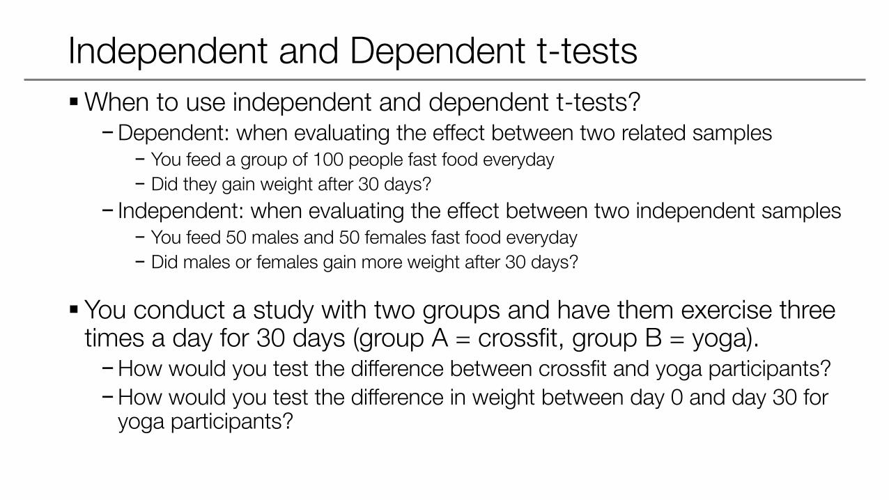
Independent and Dependent t-tests
When to use independent and dependent t-tests?−Dependent: when evaluating the effect between two related samples
− You feed a group of 100 people fast food everyday
− Did they gain weight after 30 days?
− Independent: when evaluating the effect between two independent samples− You feed 50 males and 50 females fast food everyday
− Did males or females gain more weight after 30 days?
You conduct a study with two groups and have them exercise three times a day for 30 days (group A = crossfit, group B = yoga).−How would you test the difference between crossfit and yoga participants?
−How would you test the difference in weight between day 0 and day 30 for yoga participants?

Effect Size
When samples become large enough, you often get significant results−However, is it practically significant?
Effect size is a simple way to quantify difference between two groups−Emphasizes the size of the difference (without effect of sample size)
−Cohen’s d is one of the most common ways to measure effect size
Effect size:
Proper calculation for 𝑆𝐷𝑝𝑜𝑜𝑙𝑒𝑑:
Simple calculation for 𝑆𝐷𝑝𝑜𝑜𝑙𝑒𝑑:

Time for practice
In this lab session we will cover:− Independent t-tests
−Dependent (paired) t-tests
−Effect size (Cohen’s d)
GitHub repository: https://github.com/eugeneyan/Statistical-Inference

Thank you for your attention!Eugene Yan