Sustainable it and it for sustainability

Sustainable IT and IT for Sustainability

Thesis by

Zhenhua Liu

In Partial Fulfillment of the Requirements

for the Degree of

Doctor of Philosophy

California Institute of Technology

Pasadena, California

2014

(Defended May 27, 2014)

ii

c© 2014

Zhenhua Liu

All Rights Reserved

iii

This thesis is dedicated to

my wife Zheng,

whose love made this possible,

my parents,

who have supported me all the way,

and our beloved baby.

iv

Acknowledgments

During the past five years, I have been always grateful for the extreme fortune to be co-advised by

Prof. Adam Wierman and Prof. Steven Low. It is really a luxury and indeed an honor, working with

them at this early stage of my academic career, and learning from them from critical thinking, clear

writing, effective presentations, student mentoring, time management, positive attitude, and many

others. The experience has far surpassed my expectation. Their thoughtful guidance, continuing

support without reservation, and cheerful encouragement accompanied me to hurdle all the obstacles

during the past years. They did motivate and nurture me so much that I feel even stronger than I

ever imagined. In my mind, they are the best advisors and excellent role models! It feels like such

a short five years and I still have quite a lot to learn, but it is already the time to move on. They

are my most important motivation in pursuing an academic position because I sincerely appreciate

all the amazing impacts they have had on me, and hope to extend these to others through my own

career in the future.

I am also grateful to many other collaborators all over the world. First, the past three-year

collaborations with HP Labs contribute a lot to my knowledge and skills. My mentor, Yuan Chen,

has always been patient and ready to help. We did an excellent job together with great colleagues,

including Cullen Bash, Chandrakant Patel, Daniel Gmach, Zhikui Wang, Manish Marwah, Chris

Hyser, and many others. This has been a pleasant and productive experience. Second, I would like

to thank those from Caltech: Minghong Lin, Niangjun Chen, Benjamin Razon, Iris Liu, and Katie

Knister. It has been a great pleasure working with them. In particular, I would like to thank Prof.

Mani Chandy for his insightful comments and advice. I am also thankful to my former advisors, Prof.

Youjian Zhao and Prof. Xiaoping Zhang, for their guidance during my master study in Tsinghua

University. Last but not least, I would like to take this opportunity to express my gratitude to

many others who helped me during my PhD study: Prof. Xue Liu from McGill University, Prof.

Martin Arlitt from University of Calgary and HP Labs, Prof. Jean Walrand from UC Berkeley,

Prof. Lachlan Andrew from Australia, Pablo Bauleo from Fort Collins Utilities, Yanpei Chen from

Cloudera, and Hao Wang from Google. They all contributed to this thesis from different perspectives

and significantly improved its quality.

I sincerely enjoyed studying in the Department of Computing and Mathematical Sciences at

v

Caltech, in which students rarely have to worry about anything other than our research. My in-

terdisciplinary research benefits quite a bit from Caltech’s open and friendly atmosphere. There

is hardly any barrier among different departments or colleges. I believe this contributes a lot to

our success and actually I have been actively looking for similar environment during my academic

job hunting. Additionally, I would like to thank the helpful administrative staff in our department,

especially Maria Lopez and Sydney Garstang, for keeping everything working in our favor.

Finally, my family provided me a pleasant environment, in which I can develop freely. Something

I realized just recently during my job hunting is how much my father has impacted me during my

first 19 years before college as a high school teacher in mathematics. Another thing that I already

feel so comfortable and accustomed to is the lasting understanding, support, and love from my wife,

Zheng Zhai. It is so ordinary in my daily life that I do not remember often how scarce it is and how

much I have been blessed! This thesis would not have been possible without all of these.

vi

Abstract

Energy and sustainability have become one of the most critical issues of our generation. While

the abundant potential of renewable energy such as solar and wind provides a real opportunity for

sustainability, their intermittency and uncertainty present a daunting operating challenge. This

thesis aims to develop analytical models, deployable algorithms, and real systems to enable efficient

integration of renewable energy into complex distributed systems with limited information.

The first thrust of the thesis is to make IT systems more sustainable by facilitating the integration

of renewable energy into these systems. IT represents the fastest growing sectors in energy usage

and greenhouse gas pollution. Over the last decade there are dramatic improvements in the energy

efficiency of IT systems, but the efficiency improvements do not necessarily lead to reduction in

energy consumption because more servers are demanded. Further, little effort has been put in

making IT more sustainable, and most of the improvements are from improved “engineering” rather

than improved “algorithms”. In contrast, my work focuses on developing algorithms with rigorous

theoretical analysis that improve the sustainability of IT. In particular, this thesis seeks to exploit

the flexibilities of cloud workloads both (i) in time by scheduling delay-tolerant workloads and (ii)

in space by routing requests to geographically diverse data centers. These opportunities allow data

centers to adaptively respond to renewable availability, varying cooling efficiency, and fluctuating

energy prices, while still meeting performance requirements. The design of the enabling algorithms

is however very challenging because of limited information, non-smooth objective functions and the

need for distributed control. Novel distributed algorithms are developed with theoretically provable

guarantees to enable the “follow the renewables” routing. Moving from theory to practice, I helped

HP design and implement industry’s first Net-zero Energy Data Center.

The second thrust of this thesis is to use IT systems to improve the sustainability and efficiency of

our energy infrastructure through data center demand response. The main challenges as we integrate

more renewable sources to the existing power grid come from the fluctuation and unpredictability

of renewable generation. Although energy storage and reserves can potentially solve the issues, they

are very costly. One promising alternative is to make the cloud data centers demand responsive. The

potential of such an approach is huge. To realize this potential, we need adaptive and distributed

control of cloud data centers and new electricity market designs for distributed electricity resources.

vii

My work is progressing in both directions. In particular, I have designed online algorithms with the-

oretically guaranteed performance for data center operators to deal with uncertainties under popular

demand response programs. Based on local control rules of customers, I have further designed new

pricing schemes for demand response to align the interests of customers, utility companies, and the

society to improve social welfare.

viii

Contents

Acknowledgments iv

Abstract vi

1 Introduction 1

2 Sustainable IT: Greening Geographical Load Balancing 5

2.1 Model and Notation . . . . . . . . . . . . . . . . . . . . . . . . . . . . . . . . . . . . 7

2.1.1 The workload model . . . . . . . . . . . . . . . . . . . . . . . . . . . . . . . . 7

2.1.2 The data center cost model . . . . . . . . . . . . . . . . . . . . . . . . . . . . 7

2.1.3 The geographical load balancing problem . . . . . . . . . . . . . . . . . . . . 9

2.1.4 Practical considerations . . . . . . . . . . . . . . . . . . . . . . . . . . . . . . 11

2.2 Characterizing the optima . . . . . . . . . . . . . . . . . . . . . . . . . . . . . . . . . 11

2.3 Algorithms . . . . . . . . . . . . . . . . . . . . . . . . . . . . . . . . . . . . . . . . . 12

2.4 Case study . . . . . . . . . . . . . . . . . . . . . . . . . . . . . . . . . . . . . . . . . 18

2.4.1 Experimental setup . . . . . . . . . . . . . . . . . . . . . . . . . . . . . . . . . 19

2.4.2 Performance evaluation . . . . . . . . . . . . . . . . . . . . . . . . . . . . . . 21

2.5 Social impact . . . . . . . . . . . . . . . . . . . . . . . . . . . . . . . . . . . . . . . . 24


2.5.2 The importance of dynamic pricing . . . . . . . . . . . . . . . . . . . . . . . . 25

2.6 Summary . . . . . . . . . . . . . . . . . . . . . . . . . . . . . . . . . . . . . . . . . . 27

3 Sustainable IT: System Design and Implementation 28

3.1 Sustainable Data Center Overview . . . . . . . . . . . . . . . . . . . . . . . . . . . . 30

3.1.1 Power Infrastructure . . . . . . . . . . . . . . . . . . . . . . . . . . . . . . . . 31

3.1.2 Cooling Supply . . . . . . . . . . . . . . . . . . . . . . . . . . . . . . . . . . . 32

3.1.3 IT Workload . . . . . . . . . . . . . . . . . . . . . . . . . . . . . . . . . . . . 33

3.2 Modeling and Optimization . . . . . . . . . . . . . . . . . . . . . . . . . . . . . . . . 34

3.2.1 Optimizing the cooling substructure . . . . . . . . . . . . . . . . . . . . . . . 34

ix

3.2.2 System Model . . . . . . . . . . . . . . . . . . . . . . . . . . . . . . . . . . . . 37

3.2.3 Cost and Revenue Model . . . . . . . . . . . . . . . . . . . . . . . . . . . . . 38

3.2.4 Optimization Problem . . . . . . . . . . . . . . . . . . . . . . . . . . . . . . . 39

3.2.5 Properties of the optimal workload management . . . . . . . . . . . . . . . . 40

3.3 System Prototype . . . . . . . . . . . . . . . . . . . . . . . . . . . . . . . . . . . . . . 42

3.3.1 Capacity and Workload Planner . . . . . . . . . . . . . . . . . . . . . . . . . 43

3.3.2 PV Power Forecaster . . . . . . . . . . . . . . . . . . . . . . . . . . . . . . . 45

3.3.3 IT Workload Forecaster . . . . . . . . . . . . . . . . . . . . . . . . . . . . . . 46

3.3.4 Runtime Workload Manager . . . . . . . . . . . . . . . . . . . . . . . . . . . . 47

3.4 Evaluation . . . . . . . . . . . . . . . . . . . . . . . . . . . . . . . . . . . . . . . . . . 47

3.4.1 Case Studies . . . . . . . . . . . . . . . . . . . . . . . . . . . . . . . . . . . . 47

3.4.2 Impacts of prediction errors and workload characteristics . . . . . . . . . . . 54

3.4.3 Experimental Results on a Testbed . . . . . . . . . . . . . . . . . . . . . . . . 56

3.5 Summary . . . . . . . . . . . . . . . . . . . . . . . . . . . . . . . . . . . . . . . . . . 58

4 IT for Sustainability: Data Center Demand Response 59

4.1 Coincident peak pricing . . . . . . . . . . . . . . . . . . . . . . . . . . . . . . . . . . 62

4.1.1 An overview of coincident peak pricing . . . . . . . . . . . . . . . . . . . . . . 62

4.1.2 A case study: Fort Collins Utilities Coincident Peak Pricing (CPP) Program 63

4.2 Modeling . . . . . . . . . . . . . . . . . . . . . . . . . . . . . . . . . . . . . . . . . . 66

4.2.1 Power Supply Model . . . . . . . . . . . . . . . . . . . . . . . . . . . . . . . . 67

4.2.2 Power Demand Model . . . . . . . . . . . . . . . . . . . . . . . . . . . . . . . 68

4.2.3 Total data center costs . . . . . . . . . . . . . . . . . . . . . . . . . . . . . . . 70

4.3 Algorithms . . . . . . . . . . . . . . . . . . . . . . . . . . . . . . . . . . . . . . . . . 70

4.3.1 Expected cost optimization . . . . . . . . . . . . . . . . . . . . . . . . . . . . 72

4.3.2 Robust optimization . . . . . . . . . . . . . . . . . . . . . . . . . . . . . . . . 74

4.3.3 Implementation considerations . . . . . . . . . . . . . . . . . . . . . . . . . . 76

4.4 Case study . . . . . . . . . . . . . . . . . . . . . . . . . . . . . . . . . . . . . . . . . 77


4.4.2 Experimental results . . . . . . . . . . . . . . . . . . . . . . . . . . . . . . . . 80

4.5 Summary . . . . . . . . . . . . . . . . . . . . . . . . . . . . . . . . . . . . . . . . . . 82

5 IT for Sustainability: Pricing Data Center Demand Response 84

5.1 Quantifying the potential of data center demand response . . . . . . . . . . . . . . . 88

5.1.1 Setup . . . . . . . . . . . . . . . . . . . . . . . . . . . . . . . . . . . . . . . . 88

5.1.2 Case studies . . . . . . . . . . . . . . . . . . . . . . . . . . . . . . . . . . . . . 92

5.2 Market challenges for data center demand response . . . . . . . . . . . . . . . . . . . 95

x

5.3 Prediction-based pricing for data center demand response . . . . . . . . . . . . . . . 98

5.3.1 Model formulation . . . . . . . . . . . . . . . . . . . . . . . . . . . . . . . . . 99

5.3.2 The efficiency of prediction-based pricing . . . . . . . . . . . . . . . . . . . . 100

5.3.3 Prediction-based pricing versus supply function bidding . . . . . . . . . . . . 104

5.4 Incorporating network constraints . . . . . . . . . . . . . . . . . . . . . . . . . . . . . 105

5.4.1 Modeling the network . . . . . . . . . . . . . . . . . . . . . . . . . . . . . . . 105

5.4.2 Prediction-based pricing in networks . . . . . . . . . . . . . . . . . . . . . . . 106

5.4.3 The efficiency of prediction-based pricing in networks . . . . . . . . . . . . . 108

5.5 Summary . . . . . . . . . . . . . . . . . . . . . . . . . . . . . . . . . . . . . . . . . . 110

6 Concluding remarks 111

6.1 Opportunities for data center participation in demand response programs . . . . . . 112

6.1.1 Opportunities for passive participation . . . . . . . . . . . . . . . . . . . . . . 112

6.1.2 Opportunities for active participation . . . . . . . . . . . . . . . . . . . . . . 114

6.2 Challenges that limit data center participation in demand response . . . . . . . . . . 117

6.3 Recent progress in data center demand response . . . . . . . . . . . . . . . . . . . . 118

6.3.1 Managing data center participation in demand response . . . . . . . . . . . . 119

6.3.2 Design of market programs appropriate for data centers . . . . . . . . . . . . 120

6.4 Future directions . . . . . . . . . . . . . . . . . . . . . . . . . . . . . . . . . . . . . . 121

Bibliography 123

Appendices 139

A Appendix: Proofs for Chapter 2 139

A.1 Optimality conditions . . . . . . . . . . . . . . . . . . . . . . . . . . . . . . . . . . . 139

A.2 Characterizing the optima . . . . . . . . . . . . . . . . . . . . . . . . . . . . . . . . . 141

A.3 Proofs for Algorithm 1 . . . . . . . . . . . . . . . . . . . . . . . . . . . . . . . . . . . 143



B Appendix: Proofs for Chapter 3 150

B.1 Proof of Theorem 8 . . . . . . . . . . . . . . . . . . . . . . . . . . . . . . . . . . . . . 150

B.2 Proof of Theorem 9 . . . . . . . . . . . . . . . . . . . . . . . . . . . . . . . . . . . . . 150

B.3 Proof of Theorem 10 . . . . . . . . . . . . . . . . . . . . . . . . . . . . . . . . . . . . 151

B.4 Proof of Theorem 11 . . . . . . . . . . . . . . . . . . . . . . . . . . . . . . . . . . . . 152

C Appendix: Proofs for Chapter 4 153

C.1 Proofs of Theorem 12 and 13 . . . . . . . . . . . . . . . . . . . . . . . . . . . . . . . 153

xi

D Appendix: Proofs of Chapter 5 160

D.1 Proof of Theorem 14 . . . . . . . . . . . . . . . . . . . . . . . . . . . . . . . . . . . . 160



D.4 Proof of Corollary 1 . . . . . . . . . . . . . . . . . . . . . . . . . . . . . . . . . . . . 163


xii

List of Figures

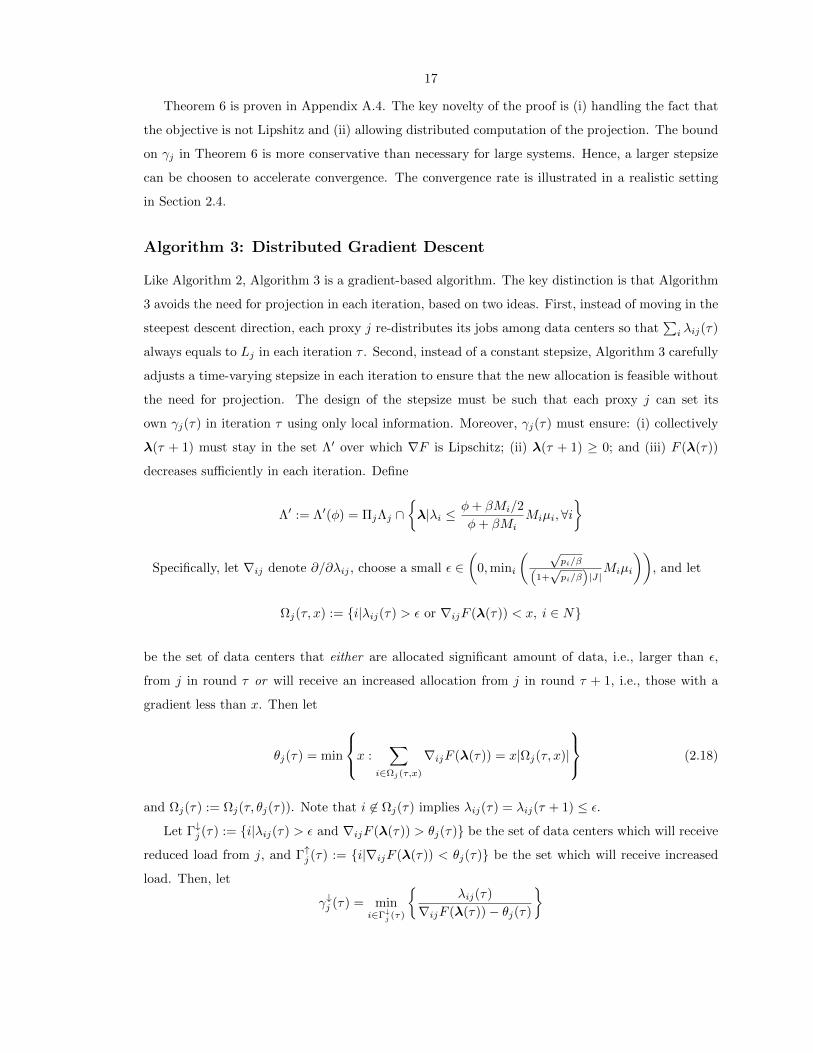
2.1 Hotmail trace used in numerical results. . . . . . . . . . . . . . . . . . . . . . . . . . . 19

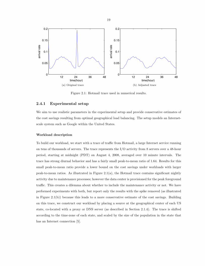
2.2 Pareto frontier of the GLB-Q formulation as a function of β for three different times

(and thus arrival rates), PDT. Circles, x-marks, and triangles correspond to β = 0.4,

1, and 2.5, respectively. . . . . . . . . . . . . . . . . . . . . . . . . . . . . . . . . . . . 20

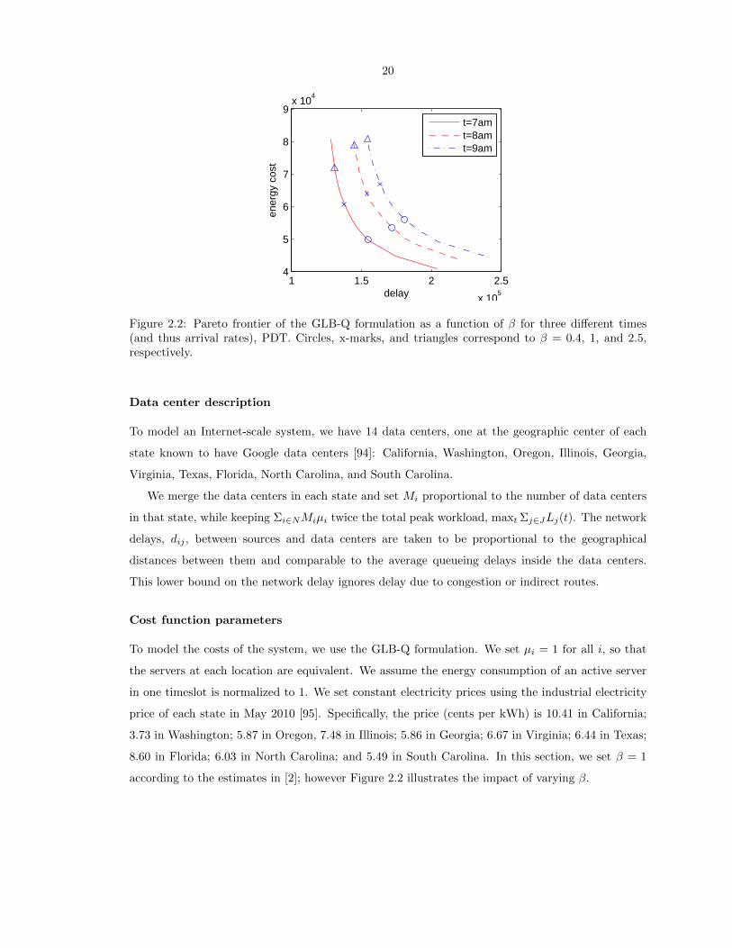
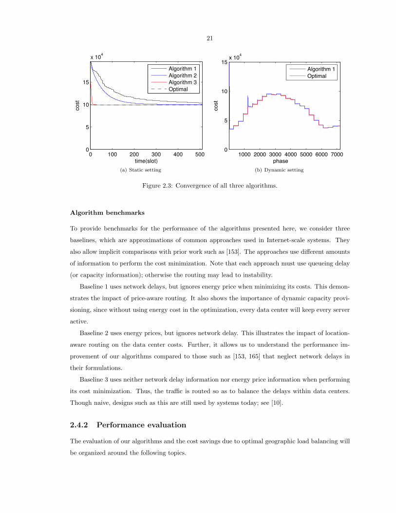
2.3 Convergence of all three algorithms. . . . . . . . . . . . . . . . . . . . . . . . . . . . . 21

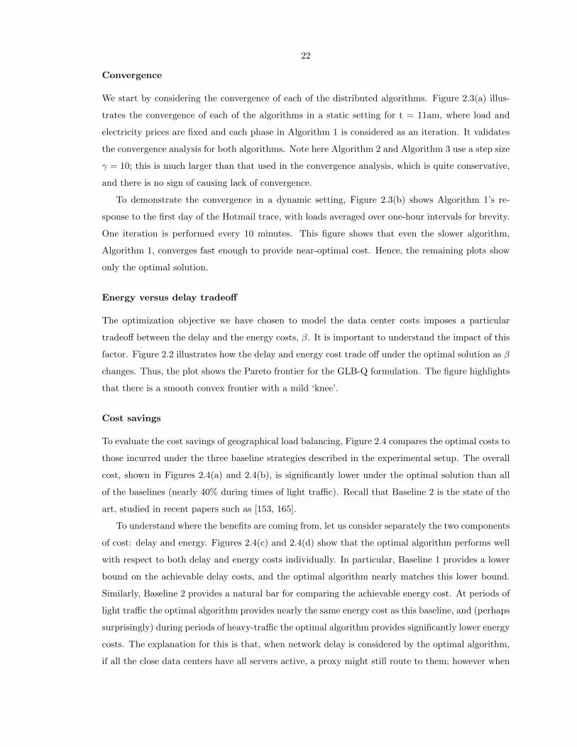
2.4 Impact of ignoring network delay and/or energy price on the cost incurred by geo-

graphical load balancing. . . . . . . . . . . . . . . . . . . . . . . . . . . . . . . . . . . 23

2.5 Geographical load balancing “following the renewables”. (a) Renewable availability.

(b) and (c): Capacity provisionings of east coast and west coast data centers when

there are renewables, under (b) optimal dynamic pricing and (c) static pricing. (d)

Reduction in social cost from dynamic pricing compared to static pricing as a function

of the weight for brown energy usage, 1/β, and β = 0.1. . . . . . . . . . . . . . . . . 26

3.1 Sustainable Data Center . . . . . . . . . . . . . . . . . . . . . . . . . . . . . . . . . . . 30

3.2 One week renewable generation . . . . . . . . . . . . . . . . . . . . . . . . . . . . . . . 31

3.3 One week real-time electricity price . . . . . . . . . . . . . . . . . . . . . . . . . . . . 32

3.4 One week interactive workload . . . . . . . . . . . . . . . . . . . . . . . . . . . . . . . 33

3.5 Cooling coefficient comparison, for conversion, 20C=68F, 25C=77F, 30C=86F . 35

3.6 Optimal cooling power . . . . . . . . . . . . . . . . . . . . . . . . . . . . . . . . . . . . 36

3.7 System Architecture . . . . . . . . . . . . . . . . . . . . . . . . . . . . . . . . . . . . . 43

3.8 PV prediction . . . . . . . . . . . . . . . . . . . . . . . . . . . . . . . . . . . . . . . . 45

3.9 Workload analysis and prediction . . . . . . . . . . . . . . . . . . . . . . . . . . . . . . 46

3.10 Power cost minimization while finishing all jobs . . . . . . . . . . . . . . . . . . . . . . 49

3.11 Benefit of cooling integration . . . . . . . . . . . . . . . . . . . . . . . . . . . . . . . . 50

3.12 Benefit of cooling optimization . . . . . . . . . . . . . . . . . . . . . . . . . . . . . . . 52

3.13 Net Zero Energy . . . . . . . . . . . . . . . . . . . . . . . . . . . . . . . . . . . . . . . 53

3.14 Optimal renewable portfolio . . . . . . . . . . . . . . . . . . . . . . . . . . . . . . . . . 54

3.15 Impact of PV prediction error . . . . . . . . . . . . . . . . . . . . . . . . . . . . . . . 55

3.16 Impact of workload prediction error . . . . . . . . . . . . . . . . . . . . . . . . . . . . 55

xiii

3.17 Impact of workload characteristics . . . . . . . . . . . . . . . . . . . . . . . . . . . . . 55

3.18 Comparison of plan and experimental results . . . . . . . . . . . . . . . . . . . . . . . 57

3.19 Comparison of optimal and night . . . . . . . . . . . . . . . . . . . . . . . . . . . . . . 58

4.1 Occurrence of coincident peak and warnings. (a) Empirical frequency of CP occurrences

on the time of day, (b) Empirical frequency of CP occurrences over the week, (c)

Empirical frequency of warning occurrences on the time of day, and (d) Empirical

frequency of warning occurrences over the week. . . . . . . . . . . . . . . . . . . . . . 64

4.2 Overview of warning occurrences showing (a) daily frequency, (b) length, and (c)-(d)

monthly frequency. . . . . . . . . . . . . . . . . . . . . . . . . . . . . . . . . . . . . . . 66

4.3 One week traces for (a) PV generation, (b) non-flexible workload demand, (c) flexible

workload demand, and (d) cooling efficiency. . . . . . . . . . . . . . . . . . . . . . . . 67

4.4 Comparison of energy costs and emissions for a data center with a local PV installation

and a local diesel generator. (a)-(j) show the plans computed by our algorithms and

the baselines. . . . . . . . . . . . . . . . . . . . . . . . . . . . . . . . . . . . . . . . . . 79

4.5 Comparison of energy costs and emissions for a data center without local generation

or PV generation. (a)-(d) show the plans computed by our algorithms. . . . . . . . . 81

4.6 Comparison of energy costs and emissions for a data center with a local PV installation,

but without local generation. (a)-(d) show the plans computed by our algorithms. . . 82

4.7 Comparison of energy costs and emissions for a data center with a local diesel generator,

but without local PV generation. (a)-(d) show the plans computed by our algorithms. 83

4.8 Sensitivity analysis of “Prediction” and “Robust” algorithms with respect to (a) work-

load and renewable generation prediction error and (b) & (c) coincident peak and

warning prediction errors. In all cases, the data center considered has a local diesel

generator, but no local PV installation. . . . . . . . . . . . . . . . . . . . . . . . . . . 83

5.1 SCE 47 bus network. . . . . . . . . . . . . . . . . . . . . . . . . . . . . . . . . . . . . . 89

5.2 SCE 56 bus network. . . . . . . . . . . . . . . . . . . . . . . . . . . . . . . . . . . . . . 89

5.3 One week traces for (a) PV generation, (b) inflexible workload, (c) flexible workload,

and (d) cooling efficiency. . . . . . . . . . . . . . . . . . . . . . . . . . . . . . . . . . . 90

5.4 Impact of energy storage capacity, Cs, on the voltage violation rates. . . . . . . . . . . 93

5.5 Impact of energy storage charging rate on the voltage violation rates. . . . . . . . . . 93

5.6 Diagram of the capacity of storage necessary to achieve the same voltage violation

frequency as data centers of varying sizes. The data center has flexibility e = 0.2. . . . 95

xiv

5.7 Comparison of a 20MW data center to large-scale storage in a 47 bus SCE distribution

network. (a)-(c) show the violation frequency as a function of the amount of data

center flexibility, e, and compare to optimally placed storage, for different locations of

the data center. (d) shows the violation frequency resulting from a data center with

e = 0.2 versus 0.33MWh of storage, for each location. . . . . . . . . . . . . . . . . . . 96

5.8 Comparison of a 4MW data center to large-scale storage in a 56 bus SCE distribu-

tion network. (a) shows the violation frequency as a function of the amount of data

center flexibility, e, and compare to optimally placed storage. (b) shows the violation

frequency resulting from a data center with e = 0.2 compared to 0.07MWh of storage

at each location. . . . . . . . . . . . . . . . . . . . . . . . . . . . . . . . . . . . . . . . 97

5.9 Comparison of a 20MW data center with a co-located 5MW PV installation to large-

scale storage in a 47 bus SCE distribution network. (a) depicts the data center located

at bus 2. (b) shows the violation frequency resulting from a data center with e = 0.2

compared to 0.33MWh of storage, for each location. . . . . . . . . . . . . . . . . . . . 98

5.10 Comparison of prediction-based pricing and supply function bidding demand response

programs. (a) shows the efficiency loss as a function of the prediction error with n = 5.

(b) shows the prediction error at which prediction-based pricing begins to have worse

efficiency than supply function bidding for each n. . . . . . . . . . . . . . . . . . . . . 105

C.1 Illustration of pdf of ε(t) that attains E[ε(t)+] = 12σε(t) for E[ε(t)] = 0 and V [ε(t)] = σ2

ε(t).157

C.2 Instance for lower bounding the competitive ratio for setting with local generation. . . 158

D.1 Diagram of cases for proof of Theorem 17. . . . . . . . . . . . . . . . . . . . . . . . . . 163

xv

List of Tables

4.1 Summary of the charging rates of Fort Collins Utilities during 2011 and 2012 [67]. . . 65

1

Chapter 1

Introduction

This thesis aims to develop analytical models, deployable algorithms, and real systems to enable

efficient integration of renewable energy into IT systems and furthermore, to use IT to improve

the sustainability and efficiency of our broad energy infrastructure through data center demand

response.

Data center demand response sits at the intersection of two important societal challenges. First,

as IT becomes increasingly crucial to society, the associated energy demands skyrocket, e.g., within

the US the growth in electricity demand of IT is ten times larger than the overall growth of elec-

tricity demands [78, 160, 110]. Second, the integration of renewable energy into the power grid is

fundamental for improving sustainability, but causes significant challenges for management of the

grid that can potentially increase costs considerably [57, 63]. Further, this challenge is magnified by

the fact that large-scale fast-charging storage is simply not cost-effective at this point.

The key idea behind data center demand response is that these two challenges are in fact symbi-

otic. Specifically, data centers are large loads, but are also flexible – data center loads can often be

shifted in time [70, 44, 120, 86, 132, 197, 193, 121], curtailed via quality degradation [20, 85, 180, 189],

or even shifted geographically [150, 153, 184, 123, 122, 188, 119, 34]. If the flexibility of data centers

can be called on by the grid via demand response programs, then they can be a crucial tool for eas-

ing the incorporation of renewable energy into the grid. Further, this interaction can be “win-win”

because the financial benefits from data center participation in demand response programs can help

ease the burden of skyrocketing energy costs.

The first thrust of the thesis is to make IT systems more sustainable by facilitating the integration

of renewable energy into these systems. IT represents the fastest growing sectors in energy usage and

greenhouse gas pollution: the Internet produces emissions comparable to the airline industry [50];

worldwide data centers consume as much electricity as United Kingdom does on an annual basis [79,

78, 160]. Most importantly, the growth rate of data center electricity usage is more than 10 times

the growth rate of the total electricity usage [78, 160, 110]. Over the last decade there are dramatic

improvements in the energy efficiency of IT systems [62, 71, 120, 185, 104, 151, 183, 23, 101, 137, 143,

2

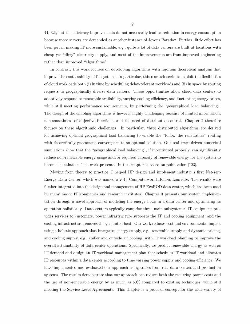
44, 32], but the efficiency improvements do not necessarily lead to reduction in energy consumption

because more servers are demanded as another instance of Jevons Paradox. Further, little effort has

been put in making IT more sustainable, e.g., quite a lot of data centers are built at locations with

cheap yet “dirty” electricity supply, and most of the improvements are from improved engineering

rather than improved “algorithms”.

In contrast, this work focuses on developing algorithms with rigorous theoretical analysis that

improve the sustainability of IT systems. In particular, this research seeks to exploit the flexibilities

of cloud workloads both (i) in time by scheduling delay-tolerant workloads and (ii) in space by routing

requests to geographically diverse data centers. These opportunities allow cloud data centers to

adaptively respond to renewable availability, varying cooling efficiency, and fluctuating energy prices,

while still meeting performance requirements, by performing the “geographical load balancing”.

The design of the enabling algorithms is however highly challenging because of limited information,

non-smoothness of objective functions, and the need of distributed control. Chapter 2 therefore

focuses on these algorithmic challenges. In particular, three distributed algorithms are derived

for achieving optimal geographical load balancing to enable the “follow the renewables” routing

with theoretically guaranteed convergence to an optimal solution. Our real trace driven numerical

simulations show that the “geographical load balancing”, if incentivized properly, can significantly

reduce non-renewable energy usage and/or required capacity of renewable energy for the system to

become sustainable. The work presented in this chapter is based on publication [123].

Moving from theory to practice, I helped HP design and implement industry’s first Net-zero

Energy Data Center, which was named a 2013 Computerworld Honors Laureate. The results were

further integrated into the design and management of HP EcoPOD data center, which has been used

by many major IT companies and research institutes. Chapter 3 presents our system implemen-

tation through a novel approach of modeling the energy flows in a data center and optimizing its

operation holistically. Data centers typically comprise three main subsystems: IT equipment pro-

vides services to customers; power infrastructure supports the IT and cooling equipment; and the

cooling infrastructure removes the generated heat. Our work reduces cost and environmental impact

using a holistic approach that integrates energy supply, e.g., renewable supply and dynamic pricing,

and cooling supply, e.g., chiller and outside air cooling, with IT workload planning to improve the

overall attainability of data center operations. Specifically, we predict renewable energy as well as

IT demand and design an IT workload management plan that schedules IT workload and allocates

IT resources within a data center according to time varying power supply and cooling efficiency. We

have implemented and evaluated our approach using traces from real data centers and production

systems. The results demonstrate that our approach can reduce both the recurring power costs and

the use of non-renewable energy by as much as 60% compared to existing techniques, while still

meeting the Service Level Agreements. This chapter is a proof of concept for the wide-variety of

3

“optimization-based designs” recently proposed, e.g., [114, 123, 153, 184, 120, 143, 122, 119]. The

work presented in this chapter is based on publication [121].

The second thrust of this thesis is to use IT systems to improve the sustainability and efficiency

of our broad energy infrastructure through data center demand response. The main challenges as

we integrate more renewable sources to the existing power grid come from the fluctuation and

unpredictability of renewable generation. Although energy storage and reserves can potentially solve

the issues, they are very costly. One promising alternative is to make geographically distributed data

centers demand responsive because it can provide significant peak demand reduction and ease the

incorporation of renewable energy into the grid. The potential of such an approach is huge. The

energy usage of cloud computing is estimated to grow at 20-30% annually over the coming decades,

which nearly matches the estimated growth rate of wind and solar installments. Data centers has a

huge potential to provide a large fraction of the amount of storage needed to incorporate renewable

resources smoothly.

To realize this potential, we need adaptive and distributed control of cloud data centers and

new electricity market designs for distributed electricity resources. My work is progressing in both

directions. Chapter 4 focuses on the design of local algorithms. In particular, we study two demand

response schemes to reduce a data center’s peak loads and energy expenditure: workload shifting and

the use of local power generation in coincident peak pricing program [67]. We develop a detailed

characterization of coincident peak data over two decades from Fort Collins Utilities, Colorado

and then design two algorithms for data centers by combining workload scheduling and local power

generation to avoid the coincident peak and reduce energy expenditure. The first algorithm optimizes

the expected cost and the second provides a good worst-case guarantee for any coincident peak

pattern, workload demand and renewable generation prediction error distributions. We evaluate

these algorithms via numerical simulations based on real world traces from production systems.

The results show that using workload shifting in combination with local generation can provide

significant cost savings compared to either alone. The work presented in this chapter is based on

publication [125].

Based on the local control rules of data centers, Chapter 5 continues to study market design for

data center demand response in order to align the interests of customers, power utility companies,

and the society to improve social welfare. Due to the market power most data centers maintain, it

is difficult to design programs that provide efficient incentives for data center demand response. To

that end, we propose that prediction-based pricing is an appealing market design, and show that it

outperforms more traditional supply function bidding mechanisms in situations where market power

is an issue. However, prediction-based pricing may be inefficient when predictions are inaccurate,

and we provide analytic, worst-case bounds on the impact of prediction error on the efficiency

of prediction-based pricing for quadratic cost functions. These bounds hold even when network

4

constraints are considered, and highlight that prediction-based pricing is surprisingly robust to

prediction errors. The work presented in this chapter is based on publication [124]. Industrial

collaborations are currently undergoing with HP, Fort Collins Utilities, and Southern California

Edison for the technology transfer.

5

Chapter 2

Sustainable IT: GreeningGeographical Load Balancing

Increasingly web services are provided by massive, geographically diverse “Internet-scale” distributed

systems, some having several data centers each with hundreds of thousands of servers. Such data

centers require many megawatts of electricity and so companies like Google and Microsoft pay tens

of millions of dollars annually for electricity [150].

The enormous, and growing, energy demands of data centers have motivated research both in

academia and industry on reducing energy usage, for both economic and environmental reasons.

Engineering advances in cooling, virtualization, DC power, etc. have led to significant improvements

in the Power Usage Effectiveness (PUE) of data centers; see [24, 170, 102, 107]. Such work focuses

on reducing the energy use of data centers and their components.

A different stream of research has focused on exploiting the geographical diversity of Internet-

scale systems to reduce the energy cost. Specifically, a system with clusters at tens or hundreds of

locations around the world can dynamically route requests/jobs to clusters based on proximity to

the user, load, and local electricity price. Thus, dynamic geographical load balancing can balance

the revenue lost due to increased delay against the electricity costs at each location.

The potential of geographical load balancing to provide significant cost savings for data centers

is well known; see [114, 143, 150, 153, 165, 184] and the references therein. The goal of the current

work is different. Our goal is to explore the social impact of geographical load balancing systems.

In particular, because GLB reduces the average price of electricity, it reduces the incentive to make

other energy-saving tradeoffs.

In contrast to this negative consequence, geographical load balancing provides a huge oppor-

tunity for environmental benefit as the penetration of green, renewable energy sources increases.

Specifically, an enormous challenge facing the electric grid is that of incorporating intermittent,

non-dispatchable renewable sources such as wind and solar. Because generation supplied to the grid

must be balanced by demand (i) instantaneously and (ii) locally (due to transmission losses and

6

the prohibitive cost of high-capacity long-distance electricity transmission lines), renewable sources

pose a significant challenge. A key technique for handling the non-dispatchability of renewable

sources is demand response, which entails the grid adjusting the demand by changing the electric-

ity price [8]. However, demand response entails a local customer curtailing use. In contrast, the

demand of Internet-scale systems is flexible geographically; thus requests can be routed to different

regions to “follow the renewables” to do the work in the right place, providing demand response

without service interruption. Since data centers represent a significant and rapidly growing fraction

of total electricity consumption, and the IT infrastructure with necessary knobs is already in place,

geographical load balancing can provide an inexpensive approach for enabling large scale, global

demand response.

The key to realizing the environmental benefits above is for data centers to move from the typical

fixed price contracts that are now widely used toward some degree of dynamic pricing, with lower

prices when renewable energy generation exceeds expectation. The current demand response markets

provide a natural way for this transition to occur, and there is already evidence of some data centers

participating in such markets [1].

The contribution of this chapter is twofold. (1) We develop distributed algorithms for geograph-

ical load balancing with provable optimality guarantees. (2) We use the proposed algorithms to

explore the feasibility and consequences of using geographical load balancing for demand response

in the grid.

Contribution (1): To derive distributed geographical load balancing algorithms we use a simple

but general model, described in detail in Section 2.1. In it, each data center minimizes its cost, which

is a linear combination of an energy cost and the lost revenue due to the delay of requests (which

includes both network propagation delay and load-dependent queueing delay within a data center).

The geographical load balancing algorithm must then dynamically decide both how requests should

be routed to data centers and how to allocate capacity in each data center (e.g., speed scaling and

how many servers are kept in active/energy-saving states).

In Section 2.2, we characterize the optimal geographical load balancing solutions and show that

they have practically appealing properties, such as sparse routing tables. In Section 2.3, we use

the previous characterization to design three distributed algorithms which provably compute the

optimal routing and provisioning decisions and require different degrees of coordination. The key

challenge here is how to design distributed algorithms with guaranteed convergence without Lipschitz

continuity. Finally, we evaluate the distributed algorithms using numeric simulation of a realistic,

distributed, Internet-scale system (Section 2.4). The results show that a cost saving of over 40%

during light-traffic periods is possible.

Contribution (2): In Section 2.5 we evaluate the feasibility and benefits of using geographical

load balancing to facilitate the integration of renewable sources into the grid. We do this using a

7

trace-driven numeric simulation of a realistic, distributed Internet-scale system in combination with

real wind and solar energy generation traces over time.

When the data center incentive is aligned with the social objective for reducing brown energy by

dynamically pricing electricity proportionally to the fraction of the total energy coming from brown

sources, we show that “follow the renewables” routing ensues (see Figure 2.5), providing significant

social benefit. We determine the wasted brown energy when prices are static, or are dynamic but

do not align data center and social objectives enough, also later shown by [72].

2.1 Model and Notation

We now introduce the workload and data center models, followed by the geographical load balancing

problem.

2.1.1 The workload model

We consider a discrete-time model with time step duration normalized to 1, such that routing and

capacity provisioning decisions can be updated within a time slot. There is a (possibly long) interval

of interest t ∈ 1, . . . , T. There are |J | geographically concentrated sources of requests, i.e., “cities”,

and work consists of jobs that arrive at a mean arrival rate of Lj(t) from source j at time t is. Jobs

are assumed to be small, so that provisioning can be based on the Lj(t). In practice, T could be a

month and a timeslot length could be 1 hour. Our analytic results make no assumptions on Lj(t);

however numerical results in Sections 2.4 and 2.5 use measured traces to define Lj(t).

2.1.2 The data center cost model

We model an Internet-scale system as a collection of |N | geographically diverse data centers, where

data center i is modeled as a collection of Mi homogeneous servers. The model focuses on two key

control decisions of geographical load balancing at each time t: (i) determining λij(t), the amount

of requests routed from source j to data center i; and (ii) determining mi(t) ∈ 0, . . . ,Mi, the

number of active servers at data center i. Since Internet data centers typically contain thousands of

active servers, we neglect the integrality constraint on mi. The system seeks to choose λij(t) and

mi(t) in order to minimize cost during [1, T ]. Depending on the system design, these decisions may

be centralized or decentralized. Section 2.3 focuses on the algorithms for this.

Our model for data center costs focuses on the server costs of the data center.1 We model costs

by combining the energy cost and the delay cost (in terms of lost revenue). Note that, to simplify

the model, we do not include the switching costs associated with cycling servers in and out of power-

1Minimizing server energy consumption also reduces cooling and power distribution costs.

8

saving modes; however, the approach of [119, 120] provides a natural way to incorporate such costs

if desired.

Energy cost. To capture the geographical diversity and variation over time of energy costs, we

let gi(t,mi, λi) denote the energy cost for data center i during timeslot t given mi active servers and

arrival rate λi including cooling power [161, 113, 121]. For every fixed t, we assume that gi(t,mi, λi)

is continuously differentiable in both mi and λi, strictly increasing in mi, non-decreasing in λi, and

jointly convex in mi and λi. This formulation is quite general. It can capture a wide range of

models for power consumption, e.g., energy costs as an affine function of the load, see [62], or as a

polynomial function of the speed, see [185, 19]2.

Defining λi(t) =∑j∈J λij(t),∀t, the total energy cost of data center i during timeslot t, denoted

by Ei(t), is simply

Ei(t) = gi(t,mi(t), λi(t)). (2.1)

Delay cost. The delay cost captures the lost revenue incurred from the delay experienced by

the requests. To model this, we define r(d) as the lost revenue associated with average delay d. We

assume that r(d) is strictly increasing and convex in d.

We consider the two components of delay: the network delay while the request is outside the

data center and the queueing delay within the data center. To model delay, we consider its two

components: the network delay experienced while the request is outside of the data center and the

queueing delay experienced in the data center.

Let dij(t) denote the average network delay of requests from source j to data center i in timeslot

t. Let fi(mi, λi) be the average queueing delay at data center i given mi active servers and an arrival

rate of λi. We assume that fi is strictly decreasing in mi, strictly increasing in λi, and strictly convex

in both mi and λi. Further, for stability, we must have that λi = 0 or λi < miµi, where µi is the

service rate of a server at data center i. Thus, we define fi(mi, λi) = ∞ for λi ≥ miµi. For other

mi, we assume fi is finite, continuous and differentiable. Note that these assumptions are satisfied

by most standard queueing formula, e.g., the average delay under M/GI/1 Processor Sharing (PS)

queue and the 95th percentile of delay under the M/M/1. Further, the convexity of fi in mi models

the law of diminishing returns for parallelism.

Combining the above gives the following model for the total delay cost Di(t) at data center i

during timeslot t:

Di(t) =∑

j∈Jλij(t)r

(fi(mi(t), λi(t)) + dij(t)

). (2.2)

2We focus on the issue of peak pricing in our recent work [125]. It requires slightly different approaches, but theycan be merged.

9

2.1.3 The geographical load balancing problem

Given the cost models above, the goal of geographical load balancing is to choose the routing policy

λij(t) and the number of active servers in each data center mi(t) at each time t in order minimize

the total cost during [1, T ]. This is captured by the following optimization problem:

minm(t),λ(t)

∑T

t=1

∑i∈N

(Ei(t) +Di(t)) (2.3a)

s.t.∑

i∈Nλij(t) = Lj(t), ∀j ∈ J (2.3b)

λij(t) ≥ 0, ∀i ∈ N, ∀j ∈ J (2.3c)

0 ≤ mi(t) ≤Mi, ∀i ∈ N (2.3d)

mi(t) ∈ N, ∀i ∈ N (2.3e)

So, we can relax the integer constraint in (2.3) and round the resulting solution with minimal

increase in cost. Because this model neglects the cost of turning servers on and off, the optimization

decouples into independent sub-problems for each timeslot t. For the analysis we consider only a

single interval.3 Thus, the minimization of the aggregate of Ei(t) + Di(i) is achieved by solving, at

each timeslot,

minm,λ

∑i∈N

gi(mi, λi) +∑i∈N

∑j∈J

λijr(dij + fi(mi, λi)) (2.4a)

s.t.∑

i∈Nλij = Lj , ∀j ∈ J (2.4b)

λij ≥ 0, ∀i ∈ N, ∀j ∈ J (2.4c)

0 ≤ mi ≤Mi, ∀i ∈ N. (2.4d)

where m = (mi)i∈N and λ = (λij)i∈N,j∈J . We refer to this formulation as GLB. Note that GLB

is jointly convex in λij and mi and can be efficiently solved centrally[31]. However, a distributed

solution algorithm is usually required by large-scale systems, such as those derived in Section 2.3.

In contrast to prior work on geographical load balancing, this work jointly optimizes total energy

cost and end-to-end user delay, with consideration of both price and network delay diversity. To our

knowledge, this is the first work to do so.

GLB provides a general framework for studying geographical load balancing. However, the model

still ignores many aspects of data center design, e.g., reliability and availability, which are central

3Time-dependence of Lj and prices is re-introduced for, and central to, the numerical results in Sections 2.4 and 2.5.

10

to data center service level agreements. Such issues are beyond the scope of this work; however our

designs merge nicely with proposals such as [168] for these goals.

The GLB model is too broad for some of our analytic results and thus we often use two restricted

versions.

Linear lost revenue. There is evidence that lost revenue is linear within the range of interest

for sites such as Google, Bing, and Shopzilla [52, 2]. To model this, we can let r(d) = βd, for

constant β. GLB then simplifies to

minm,λ

∑i∈N

gi(mi, λi)+ β

∑i∈N

λifi(mi, λi) +∑i∈N

∑j∈J

dijλij

(2.5)

subject to (2.4b)–(2.4d). We call this optimization GLB-LIN.

Queueing-based delay. We occasionally specify the form of f and g using queueing models.

This provides increased intuitions about the distributed algorithms presented.

If the workload is perfectly parallelizable, and arrivals are Poisson, then fi(mi, λi) is the average

delay of mi parallel queues, with arrival rate λi/mi. Moreover, if each queue is an M/GI/1 PS queue,

fi(mi, λi) = 1/(µi − λi/mi). We also assume gi(mi, λi) = pimi, which implies that the increase in

energy cost per timeslot for being in an active state, rather than a low-power state, is mi regardless

of λi. Note that cooling efficiency of data center i can be integrated in pi, which allows incorporation

of cooling power consumption.

Under these restrictions, the GLB formulation becomes:

minm,λ

∑i∈N

pimi + β∑j∈J

∑i∈N

λij

(1

µi − λi/mi+ dij

)(2.6a)

subject to (2.4b)–(2.4d) and the additional constraint

λi ≤ miµi ∀i ∈ N. (2.6b)

We refer to this optimization as GLB-Q.

Additional Notation. Throughout the chapter we use |S| to denote the cardinality of a set S

and bold symbols to denote vectors or tuples. In particular, λj = (λij)i∈N denotes the tuple of λij

from source j, and λ−j = (λik)i∈N,k∈J\j denotes the tuples of the remaining λik, which forms a

matrix.

We also need the following in discussing the algorithms. Define Fi(mi, λi) = gi(mi, λi) +

βλifi(mi, λi), and define F (m,λ) =∑i∈N Fi(mi, λi) + Σijλijdij . Further, let mi(λi) be the uncon-

strained optimal mi at data center i given fixed λi, i.e., the unique solution to ∂Fi(mi, λi)/∂mi = 0.

11

2.1.4 Practical considerations

Our model assumes there exist mechanisms for dynamically (i) provisioning capacity of data cen-

ters, and (ii) adapting the routing of requests from sources to data centers. With respect to (i),

many dynamic server provisioning techniques are being explored by both academics and industry,

e.g., [16, 43, 71, 173]. With respect to (ii), there are also a variety of protocol-level mechanisms

employed for data center selection today. They include, (a) dynamically generated DNS responses,

(b) HTTP redirection, and (c) using persistent HTTP proxies to tunnel requests. Each of these has

been evaluated thoroughly, e.g., [49, 131, 146, 184], and though DNS has drawbacks it remains the

preferred mechanism for many industry leaders such as Akamai, possibly due to the added latency

due to HTTP redirection and tunneling [144]. Within the GLB model, we have implicitly assumed

that there exists a proxy/DNS server co-located with each source. The practicality is also shown by

[78]. Our model also assumes that the network delays, dij can be estimated, which has been studied

extensively, including work on reducing the overhead of such measurements, e.g., [167], and mapping

and synthetic coordinate approaches, e.g., [111, 141]. We discuss the sensitivity of our algorithms

to error in these estimates in Section 2.4.

2.2 Characterizing the optima

We now provide characterizations of the optimal solutions to GLB, which are important for proving

convergence of the distributed algorithms in Section 2.3. They are also necessary because, a priori,

one might worry that the optimal solution requires a very complex routing structure, which would

be impractical; or that the set of optimal solutions is very fragmented, which would slow convergence

in practice. The results here show that such worries are unwarranted.

Uniqueness of optimal solution

To begin, note that GLB has at least one optimal solution. This can be seen by applying Weierstrass’

theorem [25], since the objective function is continuous and the feasible set is compact subset of Rn.

Although the optimal solution is generally not unique, there are natural aggregate quantities unique

over the set of optimal solutions, which is a convex set. These are the focus of this section.

A first result is that for the GLB-LIN formulation, under weak conditions on fi and gi, we have

that λi is common across all optimal solutions. Thus, the input to the data center provisioning

optimization is unique.

Theorem 1. Consider the GLB-LIN formulation. Suppose that for all i, Fi(mi, λi) is jointly convex

in λi and mi, and continuously differentiable in λi. Further, suppose that mi(λi) is strictly convex.

Then, for each i, λi is common for all optimal solutions.

12

The proofs of this subsection are in the Appendix A.2. Note that theorem 1 implies that the

server arrival rates at each data center, i.e., λi/mi, are common among all optimal solutions.

Though the conditions on Fi and mi are weak, they do not hold for GLB-Q. In that case, mi(λi)

is linear, and thus not strictly convex. Although the λi are not common across all optimal solutions

in this setting, the server arrival rates remain common across all optimal solutions.

Theorem 2. For each data center i, the server arrival rates, λi/mi, are common across all optimal

solutions to GLB-Q.

Sparsity of routing

It would be impractical if the optimal solutions to GLB required that requests from each source were

divided up among (nearly) all of the data centers. In general, each λij could be non-zero, yielding

|N |×|J | flows of requests from sources to data centers, which would lead to significant scaling issues.

Luckily, there is guaranteed to exist an optimal solution with extremely sparse routing. Specifically,

we have the following result.

Theorem 3. There exists an optimal solution to GLB with at most (|N |+ |J |−1) of the λij strictly

positive.

Though Theorem 3 does not guarantee that every optimal solution is sparse, the proof is con-

structive. Thus, it provides an approach which allows one to transform any optimal solution into a

sparse optimal one.

The following result further highlights the sparsity of the routing: any source will route to at most

one data center that is not fully active, i.e., where there exists at least one server in power-saving

mode.

Theorem 4. Consider GLB-Q where power costs pi are drawn from an arbitrary continuous dis-

tribution. If any source j ∈ J has its requests split between multiple data centers N ′ ⊆ N in an

optimal solution, then, with probability 1, at most one data center i ∈ N ′ has mi < Mi.

2.3 Algorithms

We now present three distributed algorithms and prove their convergence. For simplicity we focus

on GLB-Q; the approaches are applicable more generally, but become much more complex for richer

models.

Since GLB-Q is convex, it can be efficiently solved centrally if all necessary information can be

collected at a single point, as may be possible if all the proxies and data centers were owned by

the same system with real-time synchronization. However, there is a strong case for Internet-scale

13

systems to outsource route selection [184]. To meet this need, the algorithms presented below are

decentralized and allow each data center and proxy to optimize based on partial information.

These algorithms seek to fill a notable gap in the growing literature on algorithms for geographical

load balancing. Specifically, they have provable optimality guarantees for a performance objective

that includes both energy and delay, where route decisions are made using energy price and network

propagation delay information. The most closely related work [153] investigates the total electricity

cost for data centers in a multi-electricity-market environment. It contains the queueing delay inside

the data center (assumed to be a centralized M/M/1 queue), but neglects the end-to-end user delay.

Conversely, [184] uses a simple, efficient algorithm to coordinate the “replica-selection” decisions for

load balancing. Other related works, e.g., [153, 150, 143], either do not provide provable guarantees

or ignore diverse network delays and/or prices.

Algorithm 1: Gauss-Seidel iteration

Algorithm 1 is motivated by the observation that GLB-Q is separable in mi, and, less obviously,

also separable in λj := (λij , i ∈ N). This allows all data centers as a group and each proxy j to

iteratively solve for optimal m and λj in a distributed manner, and communicate their intermediate

results. Though distributed, Algorithm 1 requires each proxy to solve an optimization problem.

To highlight the separation between data centers and proxies, we reformulate GLB-Q as:

minλj∈Λj

minmi∈Mi

∑i∈N

(pimi +

βλiµi − λi/mi

)+ β

∑i∈N

∑j∈J

λijdij (2.7)

Mi := [0,Mi],Λj := λj |λj ≥ 0,∑i∈N

λij = Lj , λi ≤ miµi (2.8)

Since the objective and constraintsMi and Λj are separable, this can be solved separately by data

centers i and proxies j.

The iterations of the algorithm are indexed by τ , and are assumed to be fast relative to the

timeslots t. Each iteration τ is divided into |J |+1 phases. In phase 0, all data centers i concurrently

calculate mi(τ + 1) based on their own arrival rates λi(τ), by minimizing (2.7) over their own

variables mi:

minmi∈Mi

(pimi +

βλi(τ)

µi − λi(τ)/mi

), ∀i ∈ N. (2.9)

In phase j of iteration τ , proxy j minimizes (2.7) over its own variable by setting λj(τ + 1) as the

best response to m(τ + 1) and the most recent values of λ−j := (λk, k 6= j). This works because

14

proxy j depends on λ−j only through their aggregate arrival rates at data centers:

λi(τ, j) :=∑l<j

λil(τ + 1) +∑l>j

λil(τ), ∀j ∈ J. (2.10)

To compute λi(τ, j), proxy j need not obtain individual λil(τ) or λil(τ + 1) from other proxies l.

Instead, every data center i measures its local arrival rate λi(τ, j) + λij(τ) in every phase j of the

iteration τ and sends this to proxy j at the beginning of phase j. Then proxy j obtains λi(τ, j) by

subtracting its own λij(τ) from the value received from data center i. This has less overhead than

direct messaging.

In summary, Algorithm 1 works as follows (note that the minimization (2.9) has a closed form).

Here, [x]a := minx, a.

Algorithm 1. Starting from a feasible initial allocation λ(0) and the associated m(λ(0)), let

mi(τ + 1) :=

[(1 +

1√pi/β

)· λi(τ)

µi

]Mi

, ∀i ∈ N, (2.11)

λj(τ + 1) := arg minλj∈Λj

∑i∈N

λi(τ, j) + λijµi − (λi(τ, j) + λij)/mi(τ + 1)

+∑

i∈Nλijdij . (2.12)

Since GLB-Q generally has multiple optimal λ∗j , Algorithm 1 is not guaranteed to converge to

one particular optimal solution, i.e., for each proxy j, the allocation λij(τ) of job j to data centers i

may oscillate among multiple optimal allocations. However, both the optimal cost and the optimal

per-server arrival rates to data centers will converge.

Theorem 5. Let (m(τ),λ(τ)) be a sequence generated by Algorithm 1 when applied to GLB-Q.

Then

(i) Every limit point of (m(τ),λ(τ)) is optimal.

(ii) F (m(τ),λ(τ)) converges to the optimal value.

(iii) The per-server arrival rates (λi(τ)/mi(τ), i ∈ N) to data centers converge to their unique

optimal values.

The proof of Theorem 5 follows from the fact that Algorithm 1 is a modified Gauss-Seidel

iteration. This is also the reason for the requirement that the proxies update sequentially. The

details of the proof are in Appendix A.3.

Algorithm 1 assumes that there is a common clock to synchronize all actions. In practice,

updates will likely be asynchronous, with data centers and proxies updating with different frequencies

15

using possibly outdated information. The algorithm generalizes easily to this setting, though the

convergence proof is more difficult. The convergence rate of Algorithm 1 in a realistic scenario is

illustrated numerically in Section 2.4.

Algorithm 2: Distributed gradient projection

Algorithm 2 reduces the computational load on the proxies. In each iteration, instead of each proxy

solving a constrained minimization (2.12) as in Algorithm 1, Algorithm 2 takes a single step in a

descent direction. Also, while the proxies compute their λj(τ + 1) sequentially in |J | phases in

Algorithm 1, they perform their updates all at once in Algorithm 2.

To achieve this, rewrite GLB-Q as

minλj∈Λj

∑j∈J

Fj(λ) (2.13)

where F (λ) is the result of minimization of (2.7) over mi ∈ Mi given λi. As explained in the

definition of Algorithm 1, this minimization is easy: if we denote the solution to (2.11) by

mi(λi) :=

[(1 +

1√pi/β

)· λiµi

]Mi

(2.14)

then

F (λ) :=∑i∈N

(pimi(λi) +

βλiµi − λi/mi(λi)

)+ β

∑i,j

λijdij .

We now sketch the two key ideas behind Algorithm 2. The first is the standard gradient projection

idea: move in the steepest descent direction

−∇Fj(λ) := −(∂F (λ)

∂λ1j, · · · , ∂F (λ)

∂λ|N |j

)

and then project the new point into the feasible set∏j Λj with Λj given by (2.8). The standard

gradient projection algorithm will converge if ∇F (λ) is Lipschitz over∏j Λj . This condition, how-

ever, does not hold for our F because of the term βλi/(µi−λi/mi). The second idea is to construct

a compact and convex subset Λ of the feasible set∏j Λj with the following properties: (i) if the

algorithm starts in Λ, it stays in Λ; (ii) Λ contains all optimal allocations; (iii) ∇F (λ) is Lipschitz

over Λ. The algorithm then projects into Λ in each iteration instead of∏j Λj . This guarantees

convergence.

Specifically, fix a feasible initial allocation λ(0) ∈∏j Λj and let φ := F (λ(0)) be the initial

16

objective value. Define

Λ := Λ(φ) :=∏j

Λj ∩λ

∣∣∣∣λi ≤ φMiµiφ+ βMi

, ∀i. (2.15)

Even though the Λ defined in (2.15) indeed has the desired properties (see Appendix A.4), the

projection into Λ requires coordination of all proxies and is thus impractical. In order for each proxy

j to perform its update in a decentralized manner, we define proxy j’s own constraint subset:

Λj(τ) := Λj ∩λj

∣∣∣∣λi(τ,−j) + λij ≤φMiµiφ+ βMi

,∀i

where λi(τ,−j) :=∑l 6=j λil(τ) is the arrival rate to data center i, excluding arrivals from proxy j.

Even though Λj(τ) involves λi(τ,−j) for all i, proxy j can easily calculate these quantities from

data center i’s measured arrival rates λi(τ), as done in Algorithm 1 in (2.10) and the discussion

thereafter, and does not need to communicate with other proxies. Hence, given λi(τ,−j) from data

centers i, each proxy can project into Λj(τ) to compute the next iterate λj(τ + 1) without the need

to coordinate with other proxies.4 Moreover, if λ(0) ∈ Λ then λ(τ) ∈ Λ for all iterations τ .

Algorithm 2. Starting from a feasible initial allocation λ(0) and the associated m(λ(0)), each

proxy j computes, in each iteration τ :

zj(τ + 1) := [λj(τ)− γj (∇Fj(λ(τ)))]Λj(τ) , ∀j ∈ J, (2.16)

λj(τ + 1) :=|J | − 1

|J | λj(τ) +1

|J |zj(τ + 1), ∀j ∈ J. (2.17)

where γj > 0 is a stepsize.

All data centers i must compute mi(λi(τ)) according to (2.14) in each iteration τ . Each data

center i measures the local arrival rate λi(τ), calculates mi(λi(τ)), and broadcasts these values to

all proxies at the beginning of iteration τ + 1 for the proxies to compute their λj(τ + 1).

Algorithm 2 has the same convergence property as Algorithm 1, provided the stepsize is small

enough.

Theorem 6. Let (m(τ),λ(τ)) be a sequence generated by Algorithm 2 when applied to GLB-Q. If,

for all j, 0 < γj < mini∈N β2µ2iM

4i /(|J |(φ+ βMi)

3), then

(i) Every limit point of (m(τ),λ(τ)) is optimal.

(ii) F (m(τ),λ(τ)) converges to the optimal value.

(iii) The per-server arrival rates (λi(τ)/mi(τ), i ∈ N) to data centers converge to their unique

optimal values.

4The projection to the nearest point in Λj(τ) is defined by [λ]Λj(τ) := arg miny∈Λj(τ) ‖y − λ‖2.

17

Theorem 6 is proven in Appendix A.4. The key novelty of the proof is (i) handling the fact that

the objective is not Lipshitz and (ii) allowing distributed computation of the projection. The bound

on γj in Theorem 6 is more conservative than necessary for large systems. Hence, a larger stepsize

can be choosen to accelerate convergence. The convergence rate is illustrated in a realistic setting

in Section 2.4.

Algorithm 3: Distributed Gradient Descent

Like Algorithm 2, Algorithm 3 is a gradient-based algorithm. The key distinction is that Algorithm

3 avoids the need for projection in each iteration, based on two ideas. First, instead of moving in the

steepest descent direction, each proxy j re-distributes its jobs among data centers so that∑i λij(τ)

always equals to Lj in each iteration τ . Second, instead of a constant stepsize, Algorithm 3 carefully

adjusts a time-varying stepsize in each iteration to ensure that the new allocation is feasible without

the need for projection. The design of the stepsize must be such that each proxy j can set its

own γj(τ) in iteration τ using only local information. Moreover, γj(τ) must ensure: (i) collectively

λ(τ + 1) must stay in the set Λ′ over which ∇F is Lipschitz; (ii) λ(τ + 1) ≥ 0; and (iii) F (λ(τ))

decreases sufficiently in each iteration. Define

Λ′ := Λ′(φ) = ΠjΛj ∩λ|λi ≤

φ+ βMi/2

φ+ βMiMiµi,∀i

Specifically, let ∇ij denote ∂/∂λij , choose a small ε ∈(

0,mini

( √pi/β(

1+√pi/β

)|J|Miµi

)), and let

Ωj(τ, x) := i|λij(τ) > ε or ∇ijF (λ(τ)) < x, i ∈ N

be the set of data centers that either are allocated significant amount of data, i.e., larger than ε,

from j in round τ or will receive an increased allocation from j in round τ + 1, i.e., those with a

gradient less than x. Then let

θj(τ) = min

x :∑

i∈Ωj(τ,x)

∇ijF (λ(τ)) = x|Ωj(τ, x)|

(2.18)

and Ωj(τ) := Ωj(τ, θj(τ)). Note that i 6∈ Ωj(τ) implies λij(τ) = λij(τ + 1) ≤ ε.

Let Γ↓j (τ) := i|λij(τ) > ε and ∇ijF (λ(τ)) > θj(τ) be the set of data centers which will receive

reduced load from j, and Γ↑j (τ) := i|∇ijF (λ(τ)) < θj(τ) be the set which will receive increased

load. Then, let

γ↓j (τ) = mini∈Γ↓j (τ)

λij(τ)

∇ijF (λ(τ))− θj(τ)

18

be the maximum step size for which no data center will be reduced to an allocation below 0 and

γ↑j (τ) =1

|J |min

i∈Γ↑j (τ)

φ+βMi/2φ+βMi

Miµi − λi(τ)

θj(τ)−∇ijF (λ(τ))

be a lower bound on the maximum step size for which no data center will have its load increased

beyond that permitted by Λ′j(τ). Algorithm 3 proceeds as follows.

Algorithm 3. Let K ′ = maxi16|J|(φ+βMi)

3

β2M4i µ

2i

. Select % ∈ (0, 2). Starting from a feasible initial

allocation λ(0), each proxy j computes, in each iteration τ :

γj(τ) := minγ↓j (τ), γ↑j (τ), %/K ′

, (2.19)

λij(τ + 1) :=λij(τ)− γj(τ) (∇ijF (λ(τ))− θj(τ)) if i ∈ Ωj(τ)

λij(τ) ≤ ε otherwise

(2.20)

As in the case of Algorithm 2, implicit in the description is the requirement that all data centers

i compute mi(λi(τ)) according to (2.14) in each iteration τ . The procedure for this is the same as

discussed for Algorithm 2.

Theorem 7. When using Algorithm 3 in the GLB-Q formulation, F (λ(τ)) converges to a value no

greater than optimal value plus Bε, where B = β|J |∑i

((1 +

√pi/β

)2

/µi + 2 maxj dij

).

Also, as with Algorithm 2, the key novelty of the proof of Theorem 7 is the fact that we can

prove convergence even though the objective function is not Lipschitz. The proof of Theorem 7 is

provided in Appendix A.5. Finally, note that the convergence rate of Algorithm 3 is even faster

than that of Algorithm 2 in realistic settings, as we illustrate in Section 2.4. We can consider ε as

the tolerant of error when the optimal allocation λij = 0. In practice, we can set ε to a small value,

then Algorithm 3 will almost converge to the optimal value.

2.4 Case study

The remainder of the chapter evaluates the algorithms presented in the previous section under a

realistic workload. This section considers the data center perspective (i.e., cost minimization) and

Section 2.5 considers the social perspective (i.e., brown energy usage).

19

12 24 36 480

0.05

0.1

0.15

0.2

time(hour)

arriv

al ra

te

(a) Original trace

12 24 36 480

0.05

0.1

0.15

0.2

time(hour)

arriv

al ra

te

(b) Adjusted trace

Figure 2.1: Hotmail trace used in numerical results.

2.4.1 Experimental setup

We aim to use realistic parameters in the experimental setup and provide conservative estimates of

the cost savings resulting from optimal geographical load balancing. The setup models an Internet-

scale system such as Google within the United States.

Workload description

To build our workload, we start with a trace of traffic from Hotmail, a large Internet service running

on tens of thousands of servers. The trace represents the I/O activity from 8 servers over a 48-hour

period, starting at midnight (PDT) on August 4, 2008, averaged over 10 minute intervals. The

trace has strong diurnal behavior and has a fairly small peak-to-mean ratio of 1.64. Results for this

small peak-to-mean ratio provide a lower bound on the cost savings under workloads with larger

peak-to-mean ratios. As illustrated in Figure 2.1(a), the Hotmail trace contains significant nightly

activity due to maintenance processes; however the data center is provisioned for the peak foreground

traffic. This creates a dilemma about whether to include the maintenance activity or not. We have

performed experiments with both, but report only the results with the spike removed (as illustrated

in Figure 2.1(b)) because this leads to a more conservative estimate of the cost savings. Building

on this trace, we construct our workload by placing a source at the geographical center of each US

state, co-located with a proxy or DNS server (as described in Section 2.1.4). The trace is shifted

according to the time-zone of each state, and scaled by the size of the population in the state that

has an Internet connection [5].

20

1 1.5 2 2.5

x 105

4

5

6

7

8

9x 10

4

delay

ener

gy c

ost

t=7amt=8amt=9am

Figure 2.2: Pareto frontier of the GLB-Q formulation as a function of β for three different times(and thus arrival rates), PDT. Circles, x-marks, and triangles correspond to β = 0.4, 1, and 2.5,respectively.

Data center description

To model an Internet-scale system, we have 14 data centers, one at the geographic center of each

state known to have Google data centers [94]: California, Washington, Oregon, Illinois, Georgia,

Virginia, Texas, Florida, North Carolina, and South Carolina.

We merge the data centers in each state and set Mi proportional to the number of data centers

in that state, while keeping Σi∈NMiµi twice the total peak workload, maxt Σj∈JLj(t). The network

delays, dij , between sources and data centers are taken to be proportional to the geographical

distances between them and comparable to the average queueing delays inside the data centers.

This lower bound on the network delay ignores delay due to congestion or indirect routes.

Cost function parameters

To model the costs of the system, we use the GLB-Q formulation. We set µi = 1 for all i, so that

the servers at each location are equivalent. We assume the energy consumption of an active server

in one timeslot is normalized to 1. We set constant electricity prices using the industrial electricity

price of each state in May 2010 [95]. Specifically, the price (cents per kWh) is 10.41 in California;

3.73 in Washington; 5.87 in Oregon, 7.48 in Illinois; 5.86 in Georgia; 6.67 in Virginia; 6.44 in Texas;

8.60 in Florida; 6.03 in North Carolina; and 5.49 in South Carolina. In this section, we set β = 1

according to the estimates in [2]; however Figure 2.2 illustrates the impact of varying β.

21

0 100 200 300 400 5000

5

10

15

x 104

time(slot)

cost

Algorithm 1

Algorithm 2

Algorithm 3

Optimal

(a) Static setting

1000 2000 3000 4000 5000 6000 70000

5

10

15x 104

phase

cost

Algorithm 1Optimal

(b) Dynamic setting

Figure 2.3: Convergence of all three algorithms.

Algorithm benchmarks

To provide benchmarks for the performance of the algorithms presented here, we consider three

baselines, which are approximations of common approaches used in Internet-scale systems. They

also allow implicit comparisons with prior work such as [153]. The approaches use different amounts

of information to perform the cost minimization. Note that each approach must use queueing delay

(or capacity information); otherwise the routing may lead to instability.

Baseline 1 uses network delays, but ignores energy price when minimizing its costs. This demon-

strates the impact of price-aware routing. It also shows the importance of dynamic capacity provi-

sioning, since without using energy cost in the optimization, every data center will keep every server

active.

Baseline 2 uses energy prices, but ignores network delay. This illustrates the impact of location-

aware routing on the data center costs. Further, it allows us to understand the performance im-

provement of our algorithms compared to those such as [153, 165] that neglect network delays in

their formulations.

Baseline 3 uses neither network delay information nor energy price information when performing

its cost minimization. Thus, the traffic is routed so as to balance the delays within data centers.

Though naive, designs such as this are still used by systems today; see [10].

2.4.2 Performance evaluation

The evaluation of our algorithms and the cost savings due to optimal geographic load balancing will

be organized around the following topics.

22

Convergence

We start by considering the convergence of each of the distributed algorithms. Figure 2.3(a) illus-

trates the convergence of each of the algorithms in a static setting for t = 11am, where load and

electricity prices are fixed and each phase in Algorithm 1 is considered as an iteration. It validates

the convergence analysis for both algorithms. Note here Algorithm 2 and Algorithm 3 use a step size

γ = 10; this is much larger than that used in the convergence analysis, which is quite conservative,

and there is no sign of causing lack of convergence.

To demonstrate the convergence in a dynamic setting, Figure 2.3(b) shows Algorithm 1’s re-

sponse to the first day of the Hotmail trace, with loads averaged over one-hour intervals for brevity.

One iteration is performed every 10 minutes. This figure shows that even the slower algorithm,

Algorithm 1, converges fast enough to provide near-optimal cost. Hence, the remaining plots show

only the optimal solution.

Energy versus delay tradeoff

The optimization objective we have chosen to model the data center costs imposes a particular

tradeoff between the delay and the energy costs, β. It is important to understand the impact of this

factor. Figure 2.2 illustrates how the delay and energy cost trade off under the optimal solution as β

changes. Thus, the plot shows the Pareto frontier for the GLB-Q formulation. The figure highlights

that there is a smooth convex frontier with a mild ‘knee’.

Cost savings

To evaluate the cost savings of geographical load balancing, Figure 2.4 compares the optimal costs to

those incurred under the three baseline strategies described in the experimental setup. The overall

cost, shown in Figures 2.4(a) and 2.4(b), is significantly lower under the optimal solution than all

of the baselines (nearly 40% during times of light traffic). Recall that Baseline 2 is the state of the

art, studied in recent papers such as [153, 165].

To understand where the benefits are coming from, let us consider separately the two components

of cost: delay and energy. Figures 2.4(c) and 2.4(d) show that the optimal algorithm performs well

with respect to both delay and energy costs individually. In particular, Baseline 1 provides a lower

bound on the achievable delay costs, and the optimal algorithm nearly matches this lower bound.

Similarly, Baseline 2 provides a natural bar for comparing the achievable energy cost. At periods of

light traffic the optimal algorithm provides nearly the same energy cost as this baseline, and (perhaps

surprisingly) during periods of heavy-traffic the optimal algorithm provides significantly lower energy

costs. The explanation for this is that, when network delay is considered by the optimal algorithm,

if all the close data centers have all servers active, a proxy might still route to them; however when

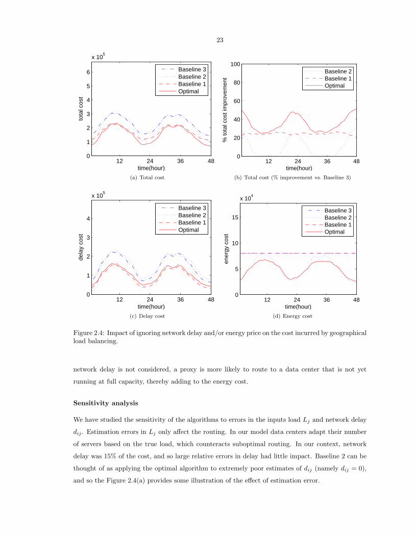
23

12 24 36 480

1

2

3

4

5

6

x 105

time(hour)

tota

l cos

t

Baseline 3Baseline 2Baseline 1Optimal

(a) Total cost

12 24 36 480

20

40

60

80

100

time(hour)

% to

tal c

ost i

mpr

ovem

ent

Baseline 2Baseline 1Optimal

(b) Total cost (% improvement vs. Baseline 3)

12 24 36 480

1

2

3

4

x 105

time(hour)

dela

y co

st


(c) Delay cost

12 24 36 480

5

10

15

x 104

time(hour)

ener

gy c

ost


(d) Energy cost

Figure 2.4: Impact of ignoring network delay and/or energy price on the cost incurred by geographicalload balancing.

network delay is not considered, a proxy is more likely to route to a data center that is not yet

running at full capacity, thereby adding to the energy cost.

Sensitivity analysis

We have studied the sensitivity of the algorithms to errors in the inputs load Lj and network delay

dij . Estimation errors in Lj only affect the routing. In our model data centers adapt their number

of servers based on the true load, which counteracts suboptimal routing. In our context, network

delay was 15% of the cost, and so large relative errors in delay had little impact. Baseline 2 can be

thought of as applying the optimal algorithm to extremely poor estimates of dij (namely dij = 0),

and so the Figure 2.4(a) provides some illustration of the effect of estimation error.

24

2.5 Social impact

We now shift focus from the cost savings of the data center operator to the social impact of geo-

graphical load balancing. We focus on the impact of geographical load balancing on the usage of

“brown” non-renewable energy by Internet-scale systems, and how this impact depends on electricity

pricing.

Intuitively, geographical load balancing allows the traffic to “follow the renewables”; thus pro-

viding increased usage of green energy and decreased brown energy usage. However, such benefits

are only possible if data centers forgo static energy contracts for dynamic energy pricing (either

through demand response programs or real-time pricing). The experiments in this section show that

if dynamic pricing is done optimally, then geographical load balancing can provide significant social

benefits by reducing non-renewable energy consumption.


To explore the social impact of geographical load balancing, we use the setup described in Section 2.4.

However, we add models for the availability of renewable energy, the pricing of renewable energy,

and the social objective.

The availability of renewable energy

To capture the availability of wind and solar energy, we use traces of wind speed and Global Hori-

zontal Irradiance (GHI) obtained from [90, 92] that have measurements every 10 minutes for a year.

The normalized generations of four states (CA, TX, IL, NC) and the West/East Coast average are

illustrated in Figure 2.5(a), where 50% of renewable energy comes from solar.

Building on these availability traces, for each location we let αi(t) denote the fraction of the

energy that is from renewable sources at time t, and let α = (|N |T )−1∑Tt=1

∑i∈N αi(t) be the

“penetration” of renewable energy. We take α = 0.30, which is on the progressive side of the

renewable targets among US states [36].

Finally, when measuring the brown/green energy usage of a data center at time t, we use simply∑i∈N αi(t)mi(t) as the green energy usage and

∑i∈N (1 − αi(t))mi(t) as the brown energy usage.

This models the fact that the grid cannot differentiate the source of the electricity provided.

Dynamic pricing and demand response

Internet-scale systems have spatial flexibility in energy usage that is not available to traditional

energy consumers; thus they are well positioned to take advantage of demand response and real-

time pricing to reduce both their electricity costs and their brown energy consumption.

25

To provide a simple model of demand response, we use time-varying prices pi(t) in each time-slot

that depend on the availability of renewable resources αi(t) in each location.

The way pi(t) is chosen as a function of αi(t) will be of fundamental importance to the social

impact of geographical load balancing. To highlight this, we consider a parameterized “differentiated

pricing” model that uses a price pb for brown energy and a price pg for green energy. Specifically,

pi(t) = pb(1− αi(t)) + pgαi(t).

Note that pg = pb corresponds to static pricing, and we show in the next section that pg = 0

corresponds to socially optimal pricing. Our experiments vary pg ∈ [0, pb]. pb is the same price as

used in Section 2.4.

The social objective

To model the social impact of geographical load balancing we need to formulate a social objective.

Like the GLB formulation, this must include a tradeoff between the energy usage and the average

delay users of the system experience, because purely minimizing brown energy use requires all

mi = 0. The key difference between the GLB formulation and the social formulation is that the cost

of energy is no longer relevant. Instead, the environmental impact is important, and thus the brown

energy usage should be minimized. This leads to the following simple model for the social objective:

minm(t),λ(t)

T∑t=1

∑i∈N

((1− αi(t))

Ei(t)pi(t)

+ βDi(t))

(2.21)

where Di(t) is the delay cost defined in (2.2), Ei(t) is the energy cost defined in (2.1), and β is the

relative valuation of delay versus energy. Further, we have imposed that the energy cost follows

from the pricing of pi(t) cents/kWh in timeslot t. Note that, though simple, our choice of Di(t) to

model the disutility of delay to users is reasonable because lost revenue captures the lack of use as

a function of increased delay.

An immediate observation about the above social objective is that to align the data center and

social goals, one needs to set pi(t) = (1 − αi(t))/β, which corresponds to choosing pb = 1/β and

pg = 0 in the differentiated pricing model above. We refer to this as the “optimal” pricing model.

2.5.2 The importance of dynamic pricing

To begin our experiments, we illustrate that optimal pricing can lead geographical load balancing

to “follow the renewables.” Figure 2.5 shows this using the renewable traces shown in Figure 2.5(a).

By comparing Figures 2.5(b) to Figure 2.5(c), which uses static pricing, the change in capacity

provisioning, and thus energy usage, is evident. For example, Figure 2.5(b) shows a clear shift of

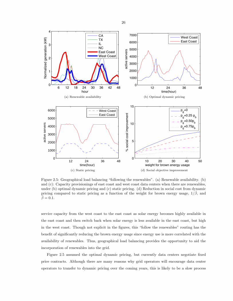
26

6 12 18 24 30 36 42 480

1

2

3

4

hour

Nor

mal

ized

gen

erat

ion

(kW

)

CATXILNCEast CoastWest Coast

(a) Renewable availability

12 24 36 480

1000

2000

3000

4000

5000

6000

7000

time(hour)

activ

e se

rver

s

West CoastEast Coast

(b) Optimal dynamic pricing

12 24 36 480

1000

2000

3000

4000

5000

6000

time(hour)

activ

e se

rver

s

West CoastEast Coast

(c) Static pricing

10 20 30 40 500

5

10

15

weight for brown energy usage

% s

ocia

l cos

t im

prov

emen

t

pg=0pg=0.25 pbpg=0.50pbpg=0.75pb

(d) Social objective improvement

Figure 2.5: Geographical load balancing “following the renewables”. (a) Renewable availability. (b)and (c): Capacity provisionings of east coast and west coast data centers when there are renewables,under (b) optimal dynamic pricing and (c) static pricing. (d) Reduction in social cost from dynamicpricing compared to static pricing as a function of the weight for brown energy usage, 1/β, andβ = 0.1.

service capacity from the west coast to the east coast as solar energy becomes highly available in

the east coast and then switch back when solar energy is less available in the east coast, but high

in the west coast. Though not explicit in the figures, this “follow the renewables” routing has the

benefit of significantly reducing the brown energy usage since energy use is more correlated with the

availability of renewables. Thus, geographical load balancing provides the opportunity to aid the

incorporation of renewables into the grid.

Figure 2.5 assumed the optimal dynamic pricing, but currently data centers negotiate fixed

price contracts. Although there are many reasons why grid operators will encourage data center

operators to transfer to dynamic pricing over the coming years, this is likely to be a slow process

27

[72]. Thus, it is important to consider the impact of partial adoption of dynamic pricing in addition

to full, optimal dynamic pricing. Figure 2.5(d) focuses on this issue. To model the partial adoption

of dynamic pricing, we can consider pg ∈ [0, pb]. This figure shows that the benefits provided by

dynamic pricing are moderate but significant, even at partial adoption (high pg). Another interesting

observation about Figure 2.5(d) is that the curves increase faster in the range when 1/β is small,

which highlights that the social benefit of geographical load balancing becomes significant even when

there is only moderate importance placed on energy. When pg is higher than pb, which is common

currently, the cost increases and geographical load balancing can no longer help to reduce non-

renewable energy consumption. We omit the results due to space considerations. For more recent

results about geographical load balancing in Internet-scale systems with local renewable generation

and data center demand response to utility coincident peak charging, please refer to [122, 125].

2.6 Summary

This chapter has focused on understanding algorithms for and social impacts of geographical load

balancing in Internet-scaled systems. We have provided three distributed algorithms that provably

compute the optimal routing and provisioning decisions for Internet-scale systems and we have

evaluated these algorithms using trace-based numerical simulations. Further, we have studied the

feasibility and benefits of providing demand response for the grid via geographical load balancing.

Our experiments highlight that geographical load balancing can provide an effective tool for demand

response: when pricing is done carefully, electricity providers can motivate Internet-scale systems

to “follow the renewables” and route to areas where green renewable energy is available. This

both eases the incorporation of non-dispatchable renewables into the grid and reduces brown energy

consumption of Internet-scale systems.

28

Chapter 3

Sustainable IT: System Design andImplementation

Data centers are emerging as the “factories” of this generation. A single data center requires a

considerable amount of electricity and data centers are proliferating worldwide as a result of increased

demand for IT applications and services. As a result, concerns about the growth in energy usage

and emissions have led to social interest in curbing their energy consumption. These concerns have

led to research efforts in both industry and academia. Emerging solutions include the incorporation

of renewable on-site energy supplies as in Apple’s new North Carolina data center, and alternative

cooling supplies as in Yahoo’s New York data center. The problem addressed by this chapter is how

to use these resources most effectively during the operation of data centers.

Most of the efforts toward this goal focus on improving the efficiency in one of the three major data

center silos: (i) IT, (ii) cooling, and (iii) power. Significant progress has been made in optimizing the

energy efficiency of each of the three silos enabling sizeable reductions in data center energy usage,

e.g., [62, 71, 120, 185, 104, 151, 183, 23]; however, the integration of these silos is an important next

step. To this end, a second generation of solutions has begun to emerge. This work focuses on the

integration of different silos [101, 137, 143, 44]. An example is the dynamic thermal management

of air-conditioners based on load at the IT rack level [101, 32]. However, to this point, supply-

side constraints such as renewable energy and cooling availability are largely treated independently

from workload management such like scheduling. Particularly, current workload management are not

designed to take advantage of time variations in renewable energy availability and cooling efficiencies.

The work in [80] integrates power capping and consolidation with renewable energy, but they do not

shift workloads to align power demand with renewable supply.

The potential of integrated, dynamic approaches has been realized in some other domains, e.g.,

cooling management solutions for buildings that predict weather and power prices to dynamically

adapt the cooling control have been proposed [9]. The goal of this chapter is to start to realize this

potential in data centers. Particularly, the potential of an integrated approach can be seen from the

29

following three observations:

First, most data centers support a range of IT workloads, including both critical interactive

applications that run 24x7 such like Internet services, and delay tolerant, batch-style applications as

scientific applications, financial analysis, and image processing, which we refer to as batch workloads

or batch jobs. Generally, batch workloads can be scheduled to run anytime as long as they finish

before deadlines. This enables significant flexibility for workload management.

Second, the availability and cost of power supply, e.g., renewable energy supply and electricity

price, is often dynamic over time, and so dynamic control of the supply mix can help reduce CO2

emissions and offset costs. Thus, thoughtful workload management can have a great impact on energy

usage and costs by scheduling batch workloads in a manner that follows the renewable availability.

Third, many data centers nowadays are cooled by multiple means through a cooling micro grid

combining traditional mechanical chillers, airside economizers, and waterside economizers. Within

a micro grid, each cooling approach has a different efficiency and capacity that depends on IT

workload, cooling generation mechanism and external conditions including outside air temperature

and humidity, and may vary with the time of day. This provides opportunities to optimize cooling

cost by “shaping” IT demand according to time varying cooling efficiency and capacity.

The three observations above highlight that there is considerable potential for integrated man-

agement of the IT, cooling, and power subsystems of data centers. Providing such an integrated

solution is the goal of this work. Specifically, we provide a novel workload scheduling and capac-

ity management approach that integrates energy supply (renewable energy supply, dynamic energy

pricing) and cooling supply (chiller cooling, outside air cooling) into IT workload management to

improve the overall energy efficiency and reduce the carbon footprint of data center operations.

A key component of our approach is demand shifting, which schedules batch workloads and

allocates IT resources within a data center according to the availability of renewable energy supply

and the efficiency of cooling. This is a complex optimization problem due to the dynamism in the

supply and demand and the interaction between them. To see this, given the lower electricity price

and temperature of outside air at night, batch jobs should be scheduled to run at night; however,

because more renewable energy like solar is available around noon, we should do more work during

the day to reduce electricity bill and environmental impact.

At the core of our design is a model of the costs within the data center, which is used to

formulate a constrained convex optimization problem. The workload planner solves this optimization

to determine the optimal demand shifting. The optimization-based workload management has been

popular in the research community recently, e.g., [114, 123, 153, 184, 120, 143, 122, 119]. The

key contributions of the formulation considered here compared to the prior literature are (i) the

addition of a detailed cost model and optimization of the cooling component of the data center,

which is typically ignored in previous designs; (ii) the consideration of both interactive and batch

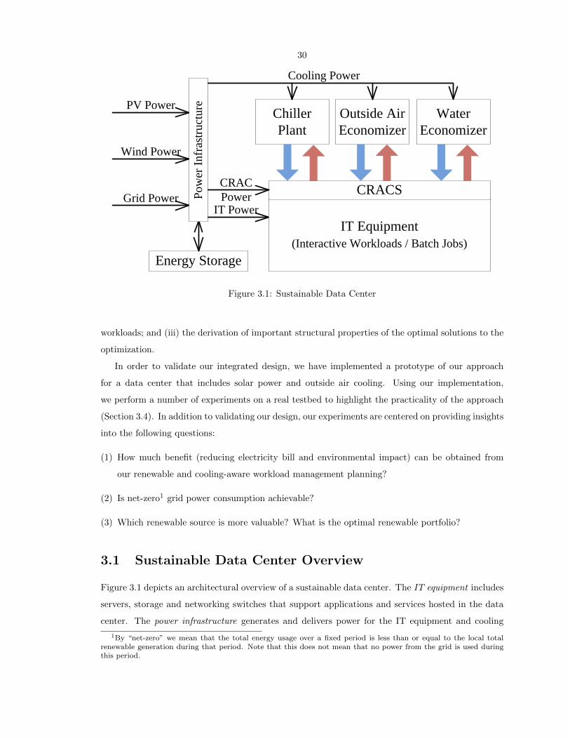
30

IT Power

Cooling Power

IT Equipment

(Interactive Workloads / Batch Jobs)

Outside Air

Economizer

Chiller

Plant

Water

Economizer

Grid Power

Wind Power

PV Power

CRACSCRAC

Power

Energy Storage

Po

wer

In

fras

tru

ctu

re

Figure 3.1: Sustainable Data Center

workloads; and (iii) the derivation of important structural properties of the optimal solutions to the

optimization.

In order to validate our integrated design, we have implemented a prototype of our approach

for a data center that includes solar power and outside air cooling. Using our implementation,

we perform a number of experiments on a real testbed to highlight the practicality of the approach

(Section 3.4). In addition to validating our design, our experiments are centered on providing insights

into the following questions:

(1) How much benefit (reducing electricity bill and environmental impact) can be obtained from

our renewable and cooling-aware workload management planning?

(2) Is net-zero1 grid power consumption achievable?

(3) Which renewable source is more valuable? What is the optimal renewable portfolio?

3.1 Sustainable Data Center Overview

Figure 3.1 depicts an architectural overview of a sustainable data center. The IT equipment includes

servers, storage and networking switches that support applications and services hosted in the data

center. The power infrastructure generates and delivers power for the IT equipment and cooling

1By “net-zero” we mean that the total energy usage over a fixed period is less than or equal to the local totalrenewable generation during that period. Note that this does not mean that no power from the grid is used duringthis period.

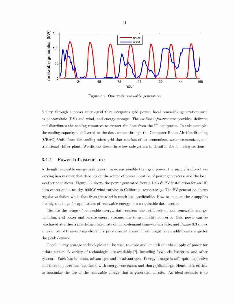
31

24 48 72 96 120 144 1680

50

100

150

hour

rene

wabl

e ge

nera

tion

(kW

)

solarwind

Figure 3.2: One week renewable generation

facility through a power micro grid that integrates grid power, local renewable generation such

as photovoltaic (PV) and wind, and energy storage. The cooling infrastructure provides, delivers,

and distributes the cooling resources to extract the heat from the IT equipment. In this example,

the cooling capacity is delivered to the data center through the Computer Room Air Conditioning

(CRAC) Units from the cooling micro grid that consists of air economizer, water economizer, and

traditional chiller plant. We discuss these three key subsystems in detail in the following sections.

3.1.1 Power Infrastructure

Although renewable energy is in general more sustainable than grid power, the supply is often time

varying in a manner that depends on the source of power, location of power generators, and the local

weather conditions. Figure 3.2 shows the power generated from a 130kW PV installation for an HP

data center and a nearby 100kW wind turbine in California, respectively. The PV generation shows

regular variation while that from the wind is much less predictable. How to manage these supplies

is a big challenge for application of renewable energy in a sustainable data center.

Despite the usage of renewable energy, data centers must still rely on non-renewable energy,

including grid power and on-site energy storage, due to availability concerns. Grid power can be

purchased at either a pre-defined fixed rate or an on-demand time-varying rate, and Figure 3.3 shows

an example of time-varying electricity price over 24 hours. There might be an additional charge for

the peak demand.

Local energy storage technologies can be used to store and smooth out the supply of power for

a data center. A variety of technologies are available [7], including flywheels, batteries, and other

systems. Each has its costs, advantages and disadvantages. Energy storage is still quite expensive

and there is power loss associated with energy conversion and charge/discharge. Hence, it is critical

to maximize the use of the renewable energy that is generated on site. An ideal scenario is to

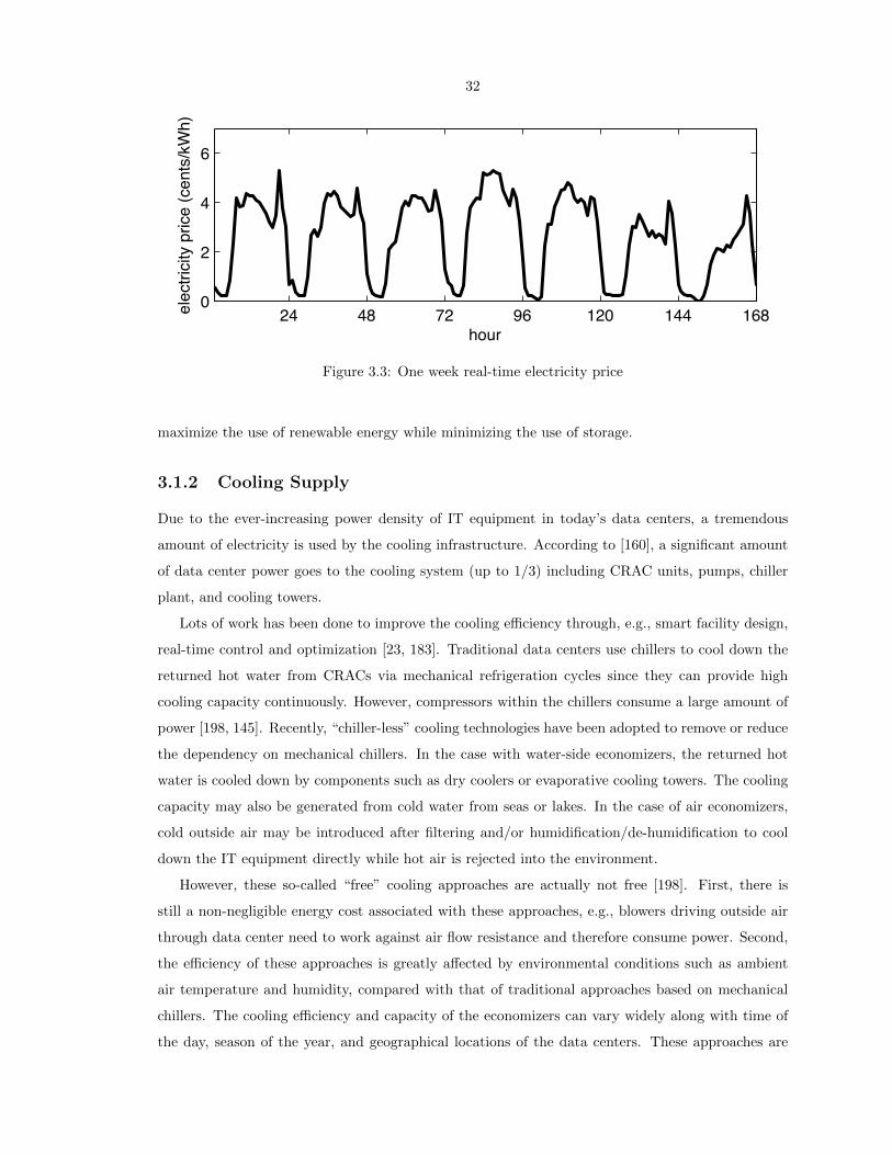
32

24 48 72 96 120 144 1680

2

4

6

hour

elec

tricit

y pr

ice (c

ents

/kW

h)

Figure 3.3: One week real-time electricity price

maximize the use of renewable energy while minimizing the use of storage.

3.1.2 Cooling Supply

Due to the ever-increasing power density of IT equipment in today’s data centers, a tremendous

amount of electricity is used by the cooling infrastructure. According to [160], a significant amount

of data center power goes to the cooling system (up to 1/3) including CRAC units, pumps, chiller

plant, and cooling towers.

Lots of work has been done to improve the cooling efficiency through, e.g., smart facility design,

real-time control and optimization [23, 183]. Traditional data centers use chillers to cool down the

returned hot water from CRACs via mechanical refrigeration cycles since they can provide high

cooling capacity continuously. However, compressors within the chillers consume a large amount of

power [198, 145]. Recently, “chiller-less” cooling technologies have been adopted to remove or reduce

the dependency on mechanical chillers. In the case with water-side economizers, the returned hot

water is cooled down by components such as dry coolers or evaporative cooling towers. The cooling

capacity may also be generated from cold water from seas or lakes. In the case of air economizers,

cold outside air may be introduced after filtering and/or humidification/de-humidification to cool

down the IT equipment directly while hot air is rejected into the environment.

However, these so-called “free” cooling approaches are actually not free [198]. First, there is

still a non-negligible energy cost associated with these approaches, e.g., blowers driving outside air

through data center need to work against air flow resistance and therefore consume power. Second,

the efficiency of these approaches is greatly affected by environmental conditions such as ambient

air temperature and humidity, compared with that of traditional approaches based on mechanical

chillers. The cooling efficiency and capacity of the economizers can vary widely along with time of

the day, season of the year, and geographical locations of the data centers. These approaches are

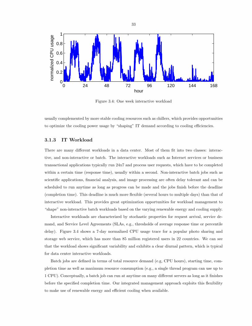
33

0 24 48 72 96 120 144 1680

0.2

0.4

0.6

0.8

1

hour

norm

aliz

ed C

PU

usa

ge

Figure 3.4: One week interactive workload

usually complemented by more stable cooling resources such as chillers, which provides opportunities

to optimize the cooling power usage by “shaping” IT demand according to cooling efficiencies.

3.1.3 IT Workload

There are many different workloads in a data center. Most of them fit into two classes: interac-

tive, and non-interactive or batch. The interactive workloads such as Internet services or business

transactional applications typically run 24x7 and process user requests, which have to be completed

within a certain time (response time), usually within a second. Non-interactive batch jobs such as

scientific applications, financial analysis, and image processing are often delay tolerant and can be

scheduled to run anytime as long as progress can be made and the jobs finish before the deadline

(completion time). This deadline is much more flexible (several hours to multiple days) than that of

interactive workload. This provides great optimization opportunities for workload management to

“shape” non-interactive batch workloads based on the varying renewable energy and cooling supply.

Interactive workloads are characterized by stochastic properties for request arrival, service de-

mand, and Service Level Agreements (SLAs, e.g., thresholds of average response time or percentile

delay). Figure 3.4 shows a 7-day normalized CPU usage trace for a popular photo sharing and

storage web service, which has more than 85 million registered users in 22 countries. We can see

that the workload shows significant variability and exhibits a clear diurnal pattern, which is typical

for data center interactive workloads.

Batch jobs are defined in terms of total resource demand (e.g, CPU hours), starting time, com-

pletion time as well as maximum resource consumption (e.g., a single thread program can use up to

1 CPU). Conceptually, a batch job can run at anytime on many different servers as long as it finishes

before the specified completion time. Our integrated management approach exploits this flexibility

to make use of renewable energy and efficient cooling when available.

34

3.2 Modeling and Optimization

As discussed above, time variations in renewable energy availability and cooling efficiencies provide

both opportunities and challenges for managing IT workloads in data centers. In this section,

we present a novel design for renewable and cooling aware workload management that exploits

opportunities available to improve the sustainability of data centers. In particular, we formulate

an optimization problem for adapting the workload scheduling and capacity allocation to varying

supply from power and cooling infrastructure.

3.2.1 Optimizing the cooling substructure

We first derive the optimal cooling substructure when multiple cooling approaches are available in

the substructure. We consider two cooling approaches: the outside air cooling which supplies most

of the cooling capacity, and cooling through mechanical chillers which guarantees availability of

cooling capacity. By exploring the heterogeneity of the efficiency and cost of the two approaches,

we represent the minimum cooling power as a function of the IT power/heat load.

In the following , we define cooling coefficient2 as the cooling power divided by the IT power to

represent the cooling efficiency. By cooling capacity we mean how much heat the cooling system can

extract from the IT equipment and reject into the environment.

Outside Air Cooling

The energy usage of outside air cooling is mainly the power consumed by blowers, which can be

approximated as a cubic function of the blower speed [30, 198]. We assume that capacity of the out-

side air cooling is under tight control, e.g., through blower speed tuning, to avoid over-provisioning.

Then the outside air capacity is equal to the IT heat load at the steady state when the latter does not

exceed the total air cooling capacity. Based on basic heat transfer theory [87], the cooling capacity

is proportional to the air volume flow rate. The air volume flow rate is approximately proportional

to blower speed according to the general fan laws [30, 198]. Therefore, outside air cooling power

can be defined as a function of IT power d as fo(d) = kd3, 0 ≤ d ≤ d, k > 0, which is a convex

function. The parameter k depends on the temperature difference, i.e., tRA − tOA, based again on

heat transfer theory, where tOA is the outside air temperature (OAT) and tRA is the temperature

of the (hot) exhausting air from the IT racks. The maximum capacity of this cooling system can

be modeled as d = C(tRA − tOA)+. (x)+ is x when it is positive and 0 otherwise. The parameter

C > 0 is the maximum cooling capacity of the air, which is proportional to the maximal outside

air mass flow rate when the blowers run at the highest speed. As one example, Figure 3.5(a) shows

the cooling coefficient for an outside air cooling system (assuming the exhausting air temperature is

2A larger cooling coefficient implies lower cooling efficiency.

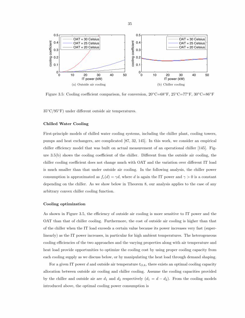
35

0 10 20 30 40 500

0.1

0.2

0.3

0.4

0.5

IT power (kW)

cool

ing

coef

ficie

nt

OAT = 30 CelsiusOAT = 25 CelsiusOAT = 20 Celsius

(a) Outside air cooling

0 10 20 30 40 500

0.1

0.2

0.3

0.4

0.5

IT power (kW)

cool

ing

coef

ficie

nt


(b) Chiller cooling

Figure 3.5: Cooling coefficient comparison, for conversion, 20C=68F, 25C=77F, 30C=86F

35C/95F) under different outside air temperatures.

Chilled Water Cooling

First-principle models of chilled water cooling systems, including the chiller plant, cooling towers,

pumps and heat exchangers, are complicated [87, 32, 145]. In this work, we consider an empirical

chiller efficiency model that was built on actual measurement of an operational chiller [145]. Fig-

ure 3.5(b) shows the cooling coefficient of the chiller. Different from the outside air cooling, the

chiller cooling coefficient does not change much with OAT and the variation over different IT load

is much smaller than that under outside air cooling. In the following analysis, the chiller power

consumption is approximated as fc(d) = γd, where d is again the IT power and γ > 0 is a constant

depending on the chiller. As we show below in Theorem 8, our analysis applies to the case of any

arbitrary convex chiller cooling function.

Cooling optimization

As shown in Figure 3.5, the efficiency of outside air cooling is more sensitive to IT power and the

OAT than that of chiller cooling. Furthermore, the cost of outside air cooling is higher than that

of the chiller when the IT load exceeds a certain value because its power increases very fast (super-

linearly) as the IT power increases, in particular for high ambient temperatures. The heterogeneous

cooling efficiencies of the two approaches and the varying properties along with air temperature and

heat load provide opportunities to optimize the cooling cost by using proper cooling capacity from

each cooling supply as we discuss below, or by manipulating the heat load through demand shaping.

For a given IT power d and outside air temperature tOA, there exists an optimal cooling capacity

allocation between outside air cooling and chiller cooling. Assume the cooling capacities provided

by the chiller and outside air are d1 and d2 respectively (d1 = d − d2). From the cooling models

introduced above, the optimal cooling power consumption is

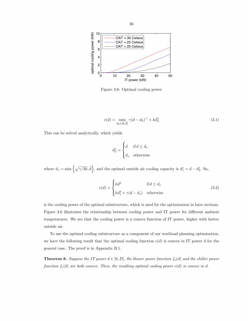
36

0 10 20 30 40 500

2

4

6

8

10

IT power (kW)

optim

al c

oolin

g po

wer (

kW)


Figure 3.6: Optimal cooling power

c(d) = mind2∈[0,d]

γ(d− d2)+ + kd32 (3.1)

This can be solved analytically, which yields

d∗2 =

d if d ≤ ds

ds otherwise

where ds = min√

γ/3k, d

, and the optimal outside air cooling capacity is d∗1 = d− d∗2. So,

c(d) =

kd3 if d ≤ ds

kd3s + γ(d− ds) otherwise

(3.2)

is the cooling power of the optimal substructure, which is used for the optimization in later sections.

Figure 3.6 illustrates the relationship between cooling power and IT power for different ambient

temperatures. We see that the cooling power is a convex function of IT power, higher with hotter

outside air.

To use the optimal cooling substructure as a component of our workload planning optimization,

we have the following result that the optimal cooling function c(d) is convex in IT power d for the

general case. The proof is in Appendix B.1.

Theorem 8. Suppose the IT power d ∈ [0, D], the blower power function fo(d) and the chiller power

function fc(d) are both convex. Then, the resulting optimal cooling power c(d) is convex in d.

37

3.2.2 System Model

We consider a discrete-time model whose timeslot matches the timescale at which the capacity

provisioning and scheduling decisions can be updated. There is a (possibly long) time period we are

interested in, 1, 2, ..., T. In practice, T could be a day and a timeslot length could be 1 hour. The

management period can be either static, e.g., to perform the scheduling every day for the execution

of the next day, or dynamic, e.g., to create a new plan if the old scheduling differs too much from

the actual supply and demand. The goal of the workload management is at each time t to:

(i) Make the scheduling decision for each batch job;

(ii) Choose the energy storage usage;

(iii) Optimize the cooling infrastructure.

We assume the renewable supply at time t is r(t), which may be a mix of different renewables,

such as wind and PV solar. We denote the grid power price at time t by p(t) and assume p(t) > 0

without loss of generality. If at some time t we have negative price, we will use up the total capacity

at this timeslot, then we only need to make capacity decisions for other timeslots. To model energy

storage, we denote the energy storage level at time t by es(t) with initial value es(0) and the

discharge/charge at time t by e(t), where positive or negative values mean discharge or charge,

respectively. Also, there is a loss rate ρ ∈ [0, 1] for energy storage. We therefore have the relation

es(t + 1) = ρ(es(t) − e(t)) between successive timeslots and we require 0 ≤ es(t) ≤ ES,∀t, where

ES is the energy storage capacity. More complex energy storage models have been considered [174],

but they are beyond the scope of this chapter.

Assume that there are I interactive workloads. For interactive workload i, the arrival rate at time

t is λi(t), the mean service rate is µi and the target performance metrics (e.g., average delay, or 95th

percentile delay) is rti. In order to satisfy these targets, we need to allocate interactive workload

i with IT capacity ai(t) at time t. Here ai(t) is derived from analytic models (e.g., M/GI/1/PS,

M/M/k) or system measurements as a function of λi(t) because performance metrics generally

improve as the capacity allocated to the workload increases, hence there is a sharp threshold for

ai(t). Note that our solution is quite general and does not depend on a particular model.

Assume there are J classes of batch jobs. Class j batch jobs have total demand Bj , maximum

parallelization MPj , starting time Sj and deadline Ej . Let bj(t) denote the amount of capacity

allocated to class j jobs at time t. We have 0 ≤ bj(t) ≤ MPj ,∀t,∀j and∑t bj(t) ≤ Bj ,∀j. Given

the above definitions, the total IT demand at time t is given by

d(t) =∑i

ai(t) +∑j

bj(t). (3.3)

38

When taking into consideration the server power model, we can further transform d(t) into power

demand, as in Section 3.3.1. We assume the total IT capacity is D, so 0 ≤ d(t) ≤ D,∀t. Note here

d(t) is not constant, but instead time-varying as a result of dynamic capacity provisioning.

Throughout the chapter we restrict our attention to situations where CPU is the major resource.

More complex resource requirements can be added as constraints, but this results in additional

complexity. Our recent work [29] shows consolidation can be achieved with only small critical

workload performance loss.

3.2.3 Cost and Revenue Model

The cost of a data center includes both capital and operating costs. Our model focuses on the

operational electricity cost. Meanwhile, by servicing the batch jobs, the data center can obtain

revenue. We model the data center cost by combining the energy cost and revenue from batch jobs.

Note that, to simplify the expression, we do not include the switching costs associated with cycling

servers in and out of power-saving modes; however, the approach of [120] provides a natural way to

incorporate such costs if desired.

To capture the variation of the energy cost over time, we let g(t, d(t), e(t)) denote the energy

cost of the data center at time t given the IT power d(t), optimal cooling power c(d(t)), renewable

generation r(t), electricity price p(t), and energy storage usage e(t). For any t, we assume that

g(t, d(t), e(t)) is non-decreasing in d(t), non-increasing in e(t), and jointly convex in d(t) and e(t).

This formulation is quite general, and captures, for example, the common charging plan of a

fixed price per kWh plus an additional “demand charge” for the peak of the average power used

over a sliding 15 minute window [142], in which case the energy cost function consists of two parts:

p(t) (d(t) + c(d(t))− r(t)− e(t))+, and

ppeak

(maxt (d(t) + c(d(t))− r(t)− e(t))+

),

where p(t) is the fixed/variable electricity price per kWh, and ppeak is the peak demand charging

rate. We could also include a sell-back mechanism and other charging policies. Additionally, this

formulation can capture a wide range of models for server power consumption, e.g., energy costs as

an affine function of the load, see [62], or as a polynomial function of the speed, see [185, 19].

We model only the variable component of the revenue3, which comes from the batch jobs that are

chosen to be run. Specifically, the data center gets revenue R(b), where b is the matrix consisting

3Revenue is also derived from the interactive workload, but for the purposes of workload management the amountof revenue from this workload is fixed.

39

of bj(t),∀j,∀t. In this chapter, we focus on the following, simple revenue function

R(b) =∑j

Rj

∑t∈[Sj ,Ej ]

bj(t)

,

where Rj is the per-job revenue.∑t∈[Sj ,Ej ]

bj(t) captures the amount of Class j jobs finished before

their deadlines.

3.2.4 Optimization Problem

We are now ready to formulate the renewable and cooling aware workload management optimization

problem. Our optimization problem takes as input the renewable supply r(t), electricity price p(t),

optimal cooling substructure c(d(t)), and IT workload demand ai(t), Bj and related information

(the starting time Sj , deadline Ej , maximum parallization MPj), IT capacity D, energy storage

capacity ES and loss rate ρ, and generates an optimal schedule of each timeslot for batch jobs bj(t)

and energy storage usage e(t), according to the availability of renewable power and cooling supply

such that specified SLAs (e.g., deadlines) and operational goals (e.g., minimizing operational costs)

are satisfied.

This is captured by the following optimization problem:

minb,e

∑t

g(t, d(t), e(t))−∑j

Rj

∑t∈[Sj ,Ej ]

bj(t)

(3.4a)

s.t.∑t

bj(t) ≤ Bj , ∀j (3.4b)

es(t+ 1) = ρ(es(t)− e(t)), ∀t (3.4c)

0 ≤ bj(t) ≤MPj , ∀j,∀t (3.4d)

0 ≤ d(t) ≤ D, ∀t (3.4e)

0 ≤ es(t) ≤ ES. ∀t (3.4f)

Here d(t) is given by (3.3). (3.4b) means the amount of served batch jobs cannot exceed the total

demand, and could become∑t bj(t) = Bj if finishing all Class j batch job is required. (3.4c)

updates the energy storage level of each timeslot. We also incorporate constraints on maximum

parallelization (3.4d), IT capacity (3.4e), and energy storage capacity (3.4f). We may have other

constraints, such as a “net zero” constraint that the total energy consumed be less than the total

renewable generation within [1, T ], i.e.,∑t(d(t)+c(d(t))) ≤

∑t r(t). Recall that our focus is on CPU

dominated workloads. When multi-dimensional workload resource requirements are necessary, we

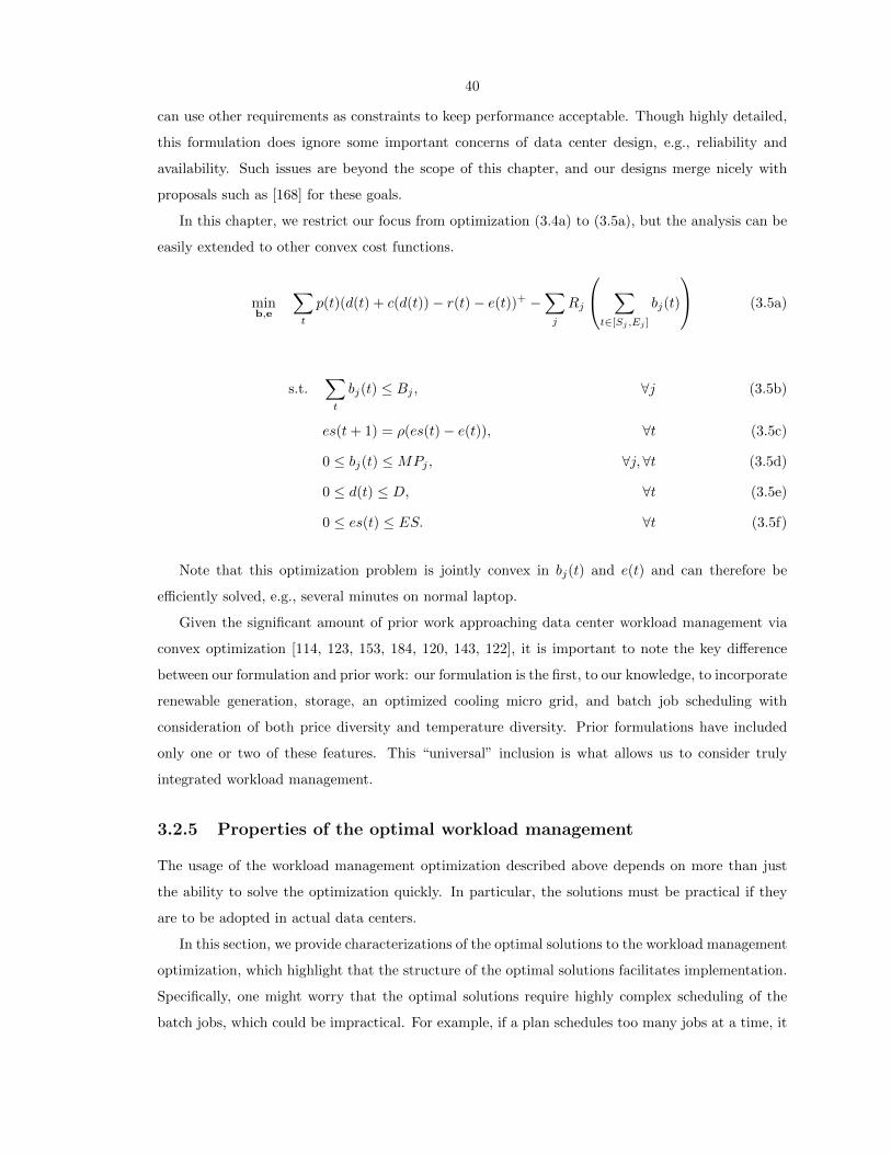
40

can use other requirements as constraints to keep performance acceptable. Though highly detailed,

this formulation does ignore some important concerns of data center design, e.g., reliability and

availability. Such issues are beyond the scope of this chapter, and our designs merge nicely with

proposals such as [168] for these goals.

In this chapter, we restrict our focus from optimization (3.4a) to (3.5a), but the analysis can be

easily extended to other convex cost functions.

minb,e

∑t

p(t)(d(t) + c(d(t))− r(t)− e(t))+ −∑j

Rj

∑t∈[Sj ,Ej ]

bj(t)

(3.5a)

s.t.∑t

bj(t) ≤ Bj , ∀j (3.5b)

es(t+ 1) = ρ(es(t)− e(t)), ∀t (3.5c)

0 ≤ bj(t) ≤MPj , ∀j,∀t (3.5d)

0 ≤ d(t) ≤ D, ∀t (3.5e)

0 ≤ es(t) ≤ ES. ∀t (3.5f)

Note that this optimization problem is jointly convex in bj(t) and e(t) and can therefore be

efficiently solved, e.g., several minutes on normal laptop.

Given the significant amount of prior work approaching data center workload management via

convex optimization [114, 123, 153, 184, 120, 143, 122], it is important to note the key difference

between our formulation and prior work: our formulation is the first, to our knowledge, to incorporate

renewable generation, storage, an optimized cooling micro grid, and batch job scheduling with

consideration of both price diversity and temperature diversity. Prior formulations have included

only one or two of these features. This “universal” inclusion is what allows us to consider truly

integrated workload management.

3.2.5 Properties of the optimal workload management

The usage of the workload management optimization described above depends on more than just

the ability to solve the optimization quickly. In particular, the solutions must be practical if they

are to be adopted in actual data centers.

In this section, we provide characterizations of the optimal solutions to the workload management

optimization, which highlight that the structure of the optimal solutions facilitates implementation.

Specifically, one might worry that the optimal solutions require highly complex scheduling of the

batch jobs, which could be impractical. For example, if a plan schedules too many jobs at a time, it

41

may not be practical because there is often an upper limit on how many workloads can be hosted

in a physical server, especially in virtualized environments. The following results show that such

concerns are unwarranted.

Energy usage and cost

Although it is easily seen that the workload management optimization problem has at least one

optimal solution,4 in general, the optimal solution is not unique. Thus, one may worry that the

optimal solutions might have very different properties with respect to energy usage and cost, which

would make capacity planning difficult. However, it turns out that the optimal solution, though not

unique, has nice properties with respect to energy usage and cost.

In particular, we prove that all optimal solutions use the same amount of power from the grid at

all times. Thus, though the scheduling of batch jobs and the usage of energy storage might be very

different, the aggregate grid power usage is always the same. This is a nice feature when considering

capacity planning of the power system. Formally, this is summarized by the following theorem,

which is proven in Appendix B.2.

Theorem 9. For the simplified energy cost model (3.5a), suppose the optimal cooling power c(d) is

strictly convex in d. Then, the energy usage from the grid, (d(t) + c(d(t)) − r(t) − e(t))+, at each

time t is common across all optimal solutions.

Though Theorem 9 considers a general setting, it is not general enough to include the optimal

cooling substructure discussed in Section 3.2.1, which includes a strictly convex section followed by a

linear section (while in practice, the chiller power is usually strictly convex in IT power, and satisfies

the requirement of Theorem 9). However, for this setting, there is a slightly weaker result that still

holds–the marginal cost of power during each timeslot is common across all optimal solutions. This

is particularly useful because it then provides the data center operator a benchmark for evaluating

which batch jobs are worthy of execution, i.e., provide marginal revenue larger than the marginal

cost they would incur. Formally, we have the following theorem, which is proven in Appendix B.3.

Theorem 10. For the simplified energy cost model (3.5a), suppose c(d) is given by (3.2). Then,

the marginal cost of power, ∂ (p(t)(d(t) + c(d(t))− r(t)− e(t))+) /∂(d(t)), at each time t is common

across all optimal solutions.

Complexity of the schedule for batch jobs

A goal of this work is to develop an efficient, implementable solution. One practical consideration is

the complexity of the schedule for batch jobs. Specifically, a schedule must not be too “fragmented”,

4This can be seen by applying Weierstrass’ theorem [25], since the objective function is continuous and the feasibleset is compact subset of Rn.

42

i.e., have many batch jobs being run at the same time and batch jobs being split across a large number

of time slots. This is particularly important in virtualized server environments because we often need

to allocate a large amount of memory for each virtual machine and the number of virtual machines

sharing a server is often limited by the memory available to virtual machines even if the CPUs can

be well shared. Additionally, there is always overhead associated with hosting virtual machines. If

we run too many virtual machines on the same server at the same time, the CPU, memory, I/O and

performance can be affected. Finally, with more virtual machines, live migrations and consolidations

during runtime management can affect the system performance.

However, it turns out that one need not worry about an overly “fragmented” schedule, since

there always exists a “simple” optimal schedule. Formally, we have the following theorem, which is

proven in Appendix B.4.

Theorem 11. There exists an optimal solution to the workload management problem with at most

(T + J − 1) of the bj(t) are neither 0 nor MPj.

Informally, this result says that there is a simple optimal solution that uses at most (T + J − 1)

more timeslots, or corresponding active virtual machines, in total than any other solutions finishing

the same number of jobs. Thus, on average, for each class of batch job per timeslot, we run at

most (T+J−1)TJ more active virtual machines than any other plan finishing the same amount of batch

jobs. Even if the number of batch job classes is small, on average, we run at most one more virtual

machine per slot. In our experiments in Section 3.4, the simplest optimal solution only uses 4% more

virtual machines. Though Theorem 11 does not guarantee that every optimal solution is simple,

the proof is constructive. Thus, it provides an approach that allows one to transform an optimal

solution into the simplest optimal solution.

In addition to Theorem 11, there are two other properties of the optimal solution that highlight

its simplicity. We state these without proof due to space consideration. First, when multiple classes

of batch jobs are served in the same timeslot, all of them except possibly the one with the lowest

revenue are eventually finished. Second, in every timeslot, the lowest marginal revenue of a batch

job that is served is still no lower than the marginal cost of power from Theorem 10.

3.3 System Prototype

We have designed and implemented a supply-aware workload and capacity management prototype

in a production data center based on the description in the previous section. The data center

is equipped with on-site PV power generation and outside air cooling. The prototype includes

workload and capacity planning, runtime workload scheduling and resource allocation, renewable

generation and IT workload demand prediction. Figure 3.7 depicts the system architecture. The

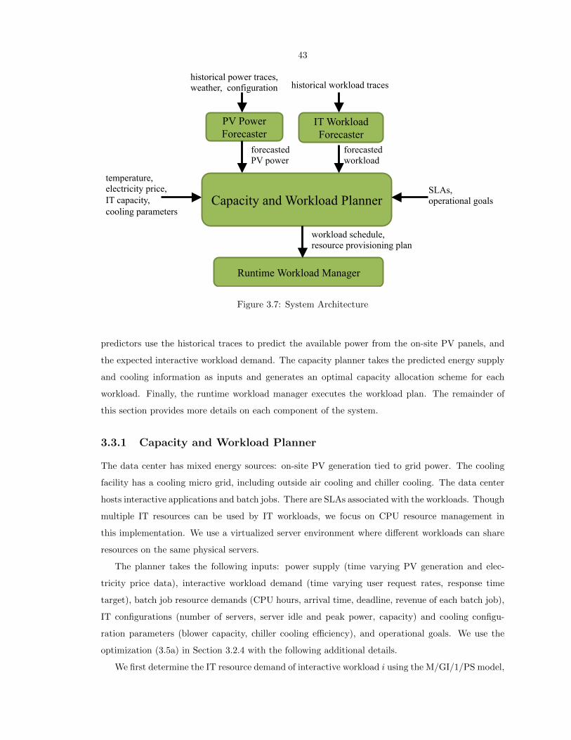
43

historical power traces, weather, configuration

forecasted PV power

forecasted workload

temperature, electricity price, IT capacity, cooling parameters

historical workload traces

workload schedule, resource provisioning plan

PV Power Forecaster

Capacity and Workload Planner

Runtime Workload Manager

IT Workload Forecaster

SLAs, operational goals

Figure 3.7: System Architecture

predictors use the historical traces to predict the available power from the on-site PV panels, and

the expected interactive workload demand. The capacity planner takes the predicted energy supply

and cooling information as inputs and generates an optimal capacity allocation scheme for each

workload. Finally, the runtime workload manager executes the workload plan. The remainder of

this section provides more details on each component of the system.

3.3.1 Capacity and Workload Planner

The data center has mixed energy sources: on-site PV generation tied to grid power. The cooling

facility has a cooling micro grid, including outside air cooling and chiller cooling. The data center

hosts interactive applications and batch jobs. There are SLAs associated with the workloads. Though

multiple IT resources can be used by IT workloads, we focus on CPU resource management in

this implementation. We use a virtualized server environment where different workloads can share

resources on the same physical servers.

The planner takes the following inputs: power supply (time varying PV generation and elec-

tricity price data), interactive workload demand (time varying user request rates, response time

target), batch job resource demands (CPU hours, arrival time, deadline, revenue of each batch job),

IT configurations (number of servers, server idle and peak power, capacity) and cooling configu-

ration parameters (blower capacity, chiller cooling efficiency), and operational goals. We use the

optimization (3.5a) in Section 3.2.4 with the following additional details.

We first determine the IT resource demand of interactive workload i using the M/GI/1/PS model,

44

which gives 1µi−λi(t)/ai(t) ≤ rti. Thus, the minimum CPU capacity needed is ai(t) = λi(t)

µi−1/rti, which

is a linear function of the arrival rate λi(t). We estimate µi through real measurements and set

the response time requirement rti according to the SLAs. While the model is not perfect for real-

world data center workloads, it provides a good approximation. Although important, performance

modeling is not the focus of this chapter. The resulting average CPU utilization of interactive

workload i is 1− 1µirti

, therefore its actual CPU usage at time t is ai(t) (1− 1/µirti), the remaining

ai(t)/µirti capacity can be shared by batch jobs. For Class j batch job, assume at time t it shares

nji(t) ≥ 0 CPU resource with interactive workload i and uses additional nj(t) ≥ 0 CPU resource

by itself, then its total CPU usage at time t is bj(t) =∑i nji(t) + nj(t), which is used to update

Constraint (4.6c) and (4.6d). We have an additional constraint on CPU capacity that can be shared∑j nji(t) ≤ ai(t)/µirti. Assume the data center has D CPU capacity in total, so the IT capacity

constraint becomes∑i ai(t) +

∑j nj(t) ≤ D. Although our optimization (3.5a) in Section 3.2.4 can

be used to handle IT workload with multi-dimensional demand, e.g., CPU, memory, here we restrict

our attention to CPU-bound workloads.

The next step is to estimate the IT power consumption, which can be done based on the average

CPU utilization

Pserver(u) = Pi + (Pb − Pi) ∗ u

where u is the average CPU utilization across all servers, Pi and Pb are the power consumed by the

server at idle and their fully utilized state, respectively. This simple model has proven very useful

and accurate in modeling power consumption since other components’ activities are either static or

correlate well with CPU activity [62]. Assuming each server has Q CPU capacity, using the above

model, we estimate the IT power as follows5:

d(t) =

∑i ai(t)

Q(Pi + (Pb − Pi) ∗ ui(t)) +

∑j nj(t)

QPb,

where ui(t) =(

1− 1µirti

+∑j nji(t)

ai(t)

).

The cooling power can be derived from the IT power according to the cooling model (3.2)

described in Section 3.2.1.

By solving the optimization problem (3.5a), we then obtain a detailed capacity plan, including

at each time t the capacity allocated to each class of batch jobs bj(t) (from both nji(t) and nj(t)),

capacity allocated to interactive workload i ai(t), energy storage usage e(t), as well as optimal cooling

configuration (i.e., capacity for outside air cooling and chiller cooling).

It follows from Section 3.2.4 that this problem is a convex optimization problem and hence there

exist efficient algorithms to solve this problem. For example, disciplined convex programming [89]

5Since the number of servers used by an interactive workload or a class of batch jobs is usually large in data centers,we treat it as continuous.

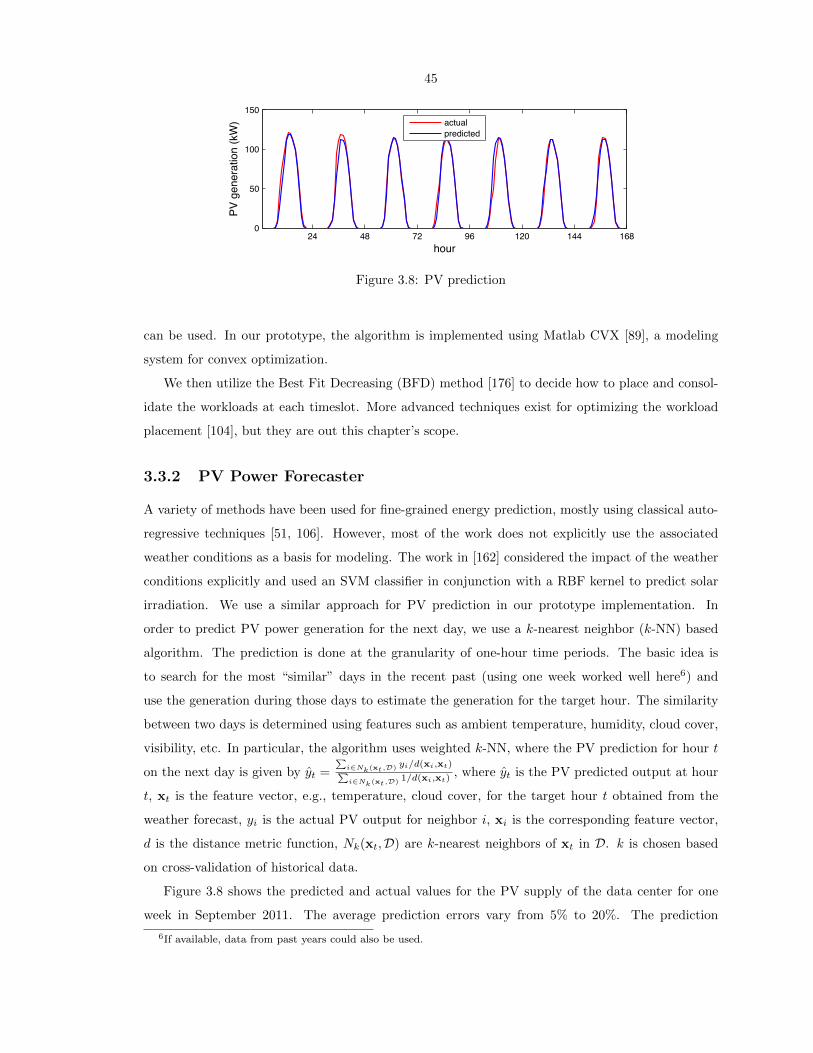
45

24 48 72 96 120 144 1680

50

100

150

hourPV

gen

erat

ion

(kW

)

actualpredicted

Figure 3.8: PV prediction

can be used. In our prototype, the algorithm is implemented using Matlab CVX [89], a modeling

system for convex optimization.

We then utilize the Best Fit Decreasing (BFD) method [176] to decide how to place and consol-

idate the workloads at each timeslot. More advanced techniques exist for optimizing the workload

placement [104], but they are out this chapter’s scope.

3.3.2 PV Power Forecaster

A variety of methods have been used for fine-grained energy prediction, mostly using classical auto-

regressive techniques [51, 106]. However, most of the work does not explicitly use the associated

weather conditions as a basis for modeling. The work in [162] considered the impact of the weather

conditions explicitly and used an SVM classifier in conjunction with a RBF kernel to predict solar

irradiation. We use a similar approach for PV prediction in our prototype implementation. In

order to predict PV power generation for the next day, we use a k-nearest neighbor (k-NN) based

algorithm. The prediction is done at the granularity of one-hour time periods. The basic idea is

to search for the most “similar” days in the recent past (using one week worked well here6) and

use the generation during those days to estimate the generation for the target hour. The similarity

between two days is determined using features such as ambient temperature, humidity, cloud cover,

visibility, etc. In particular, the algorithm uses weighted k-NN, where the PV prediction for hour t

on the next day is given by yt =∑i∈Nk(xt,D) yi/d(xi,xt)∑i∈Nk(xt,D) 1/d(xi,xt)

, where yt is the PV predicted output at hour

t, xt is the feature vector, e.g., temperature, cloud cover, for the target hour t obtained from the

weather forecast, yi is the actual PV output for neighbor i, xi is the corresponding feature vector,

d is the distance metric function, Nk(xt,D) are k-nearest neighbors of xt in D. k is chosen based

on cross-validation of historical data.

Figure 3.8 shows the predicted and actual values for the PV supply of the data center for one

week in September 2011. The average prediction errors vary from 5% to 20%. The prediction

6If available, data from past years could also be used.

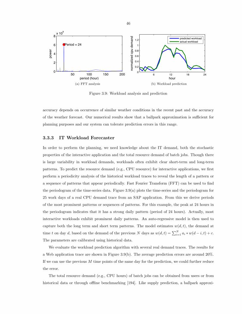
46

50 100 150 2000

2

4

6

8x 109

period (hour)

powe

rPeriod = 24

(a) FFT analysis

6 12 18 240

0.2

0.4

0.6

0.8

1

1.2

hour

norm

alize

d cp

u de

man

d

predicted workloadactual workload

(b) Workload prediction

Figure 3.9: Workload analysis and prediction

accuracy depends on occurrence of similar weather conditions in the recent past and the accuracy

of the weather forecast. Our numerical results show that a ballpark approximation is sufficient for

planning purposes and our system can tolerate prediction errors in this range.

3.3.3 IT Workload Forecaster

In order to perform the planning, we need knowledge about the IT demand, both the stochastic

properties of the interactive application and the total resource demand of batch jobs. Though there

is large variability in workload demands, workloads often exhibit clear short-term and long-term

patterns. To predict the resource demand (e.g., CPU resource) for interactive applications, we first

perform a periodicity analysis of the historical workload traces to reveal the length of a pattern or

a sequence of patterns that appear periodically. Fast Fourier Transform (FFT) can be used to find

the periodogram of the time-series data. Figure 3.9(a) plots the time-series and the periodogram for

25 work days of a real CPU demand trace from an SAP application. From this we derive periods

of the most prominent patterns or sequences of patterns. For this example, the peak at 24 hours in

the periodogram indicates that it has a strong daily pattern (period of 24 hours). Actually, most

interactive workloads exhibit prominent daily patterns. An auto-regressive model is then used to

capture both the long term and short term patterns. The model estimates w(d, t), the demand at

time t on day d, based on the demand of the previous N days as w(d, t) =∑Ni=1 ai ∗w(d− i, t) + c.

The parameters are calibrated using historical data.

We evaluate the workload prediction algorithm with several real demand traces. The results for

a Web application trace are shown in Figure 3.9(b). The average prediction errors are around 20%.

If we can use the previous M time points of the same day for the prediction, we could further reduce

the error.

The total resource demand (e.g., CPU hours) of batch jobs can be obtained from users or from

historical data or through offline benchmarking [194]. Like supply prediction, a ballpark approxi-

47

mation is good enough.

3.3.4 Runtime Workload Manager

The runtime workload manager schedules workloads and allocates CPU resource according to the

plan generated by the planner. We implement a prototype in a KVM-based virtualized server

environment [3]. Our current implementation uses a KVM/QEMU hypervisor along with control

groups (Cgroups), a new Linux feature, to perform resource allocation and workload management [3].

In particular, it executes the following tasks according to the plan: (1) create and start virtual

machines hosting batch jobs; (2) adjust the resource allocation (e.g., CPU shares or number of virtual

CPUs) to each virtual machine; (3) migrate and consolidate virtual machines via live migration. The

workload manager assigns a much higher priority to virtual machines running interactive workloads

than virtual machines for batch jobs via Cgroups. This guarantees that resources are available as

needed by interactive applications, while excess resources can be used by the batch jobs, improving

server utilization.

3.4 Evaluation

To highlight the benefits of our design for renewable and cooling aware workload management, we

perform a mixture of numerical simulations and experiments in a testbed. We first present trace-

based simulation results in Section 3.4.1 and Section 3.4.2, and then the experimental results on the

testbed implementation in Section 3.4.3.

3.4.1 Case Studies

We begin by discussing evaluations of our workload and capacity planning using numerical simu-

lations. We use traces from real data centers. In particular, we obtain PV supply, interactive IT

workload, and cooling data from real data center traces. The renewable energy and cooling data

is from measurements of one of HP’s data centers in California. The data center is equipped with

130kW PV panel array and a cooling system consisting of outside air cooling and chiller cooling.

We use the real-time electricity price of the data center location obtained from [96]. The total IT

capacity is 500 servers (100kW). The interactive workload is a popular web service application with

more than 85 million registered users in 22 countries. The trace contains average CPU utilization

and memory usage as recorded every 5 minutes. Additionally, we assume that there are a number

of batch jobs. Half of them are submitted at midnight and another half are submitted around noon.

The total demand ratio between the interactive workload and batch jobs is 1:1.5. The interactive

workload is deemed critical and the resource demand must be met while the batch jobs can be

48

rescheduled as long as they finish before their deadlines. The plan period is 24-hours and the capac-

ity planner creates a plan for the next 24-hours at midnight based on renewable supply and cooling

information as well as the interactive demand. The plan includes hourly capacity allocation for each

workload. We assume perfect knowledge about the workload demand and renewable supply, and

we study the impact of prediction errors and the mix of interactive and batch workloads in Section

3.4.2.

We explore the following issues: (i) How valuable is renewable and cooling aware workload

management? (ii) Is net-zero possible under renewable and cooling aware workload management?

(iii) What mix of wind and solar can provide most benefit?

How valuable is renewable and cooling aware workload management?

We start with the key question for this chapter: how much cost/energy/CO2 savings does renewable

and cooling aware workload management provide? In this study, we assume half of batch jobs

must be finished before noon and another half must be finished before midnight. We compare the

following four approaches: (i) Optimal, which integrates supply and cooling information and uses

our optimization algorithm to schedule batch jobs; (ii) Night, which schedules batch jobs at night to

avoid interfering with critical workloads and to take advantage of idle machines (this is a widely used

solution in practice); (iii) Best Effort (BE), which runs batch jobs immediately when they arrive

and uses all available IT to finish batch jobs as quickly as possible; (iv) Flat, which runs batch jobs

at a constant rate within the deadline period.

Figure 3.10 shows the detailed schedule and power consumption for each approach, including

IT power (batch and interactive workloads), cooling, and supply, as well as the energy usage and

efficiency comparisons. As shown in the figure, compared with other approaches, Optimal reshapes

the batch job demand and fully utilizes the renewable supply, and uses non-renewable energy, if

necessary, to complete the batch jobs during this 24-hour period. These additional batch jobs are

scheduled to run between 3am and 6am or between 11pm and midnight, when the outside air cooling

is most efficient and/or the electricity price is lower. As a result, our solution reduces the grid power

consumption by 39%-63% compared to other approaches (Figure 3.10(e)). Though not clear in the

figure, the optimal solution does consume a bit more total power (up to 2%) because of the low

cooling efficiency around noon. Figure 3.10(f) shows the average recurring electricity cost and CO2

emission per job. The energy cost per job is reduced by 53%-83% and the CO2 emission per job is

reduced by 39%-63% under the Optimal schedule. Note here we use time-varying electricity price,

so energy cost and energy consumption are not identical.

The importance of cooling aware scheduling: The adaptation of the workload management to

the availability of renewable energy is clear in Figure 3.10. Less clear is the importance of managing

the workload in a manner that is “cooling aware”. As discussed in Sections 3.1.2 and 3.2.1, the

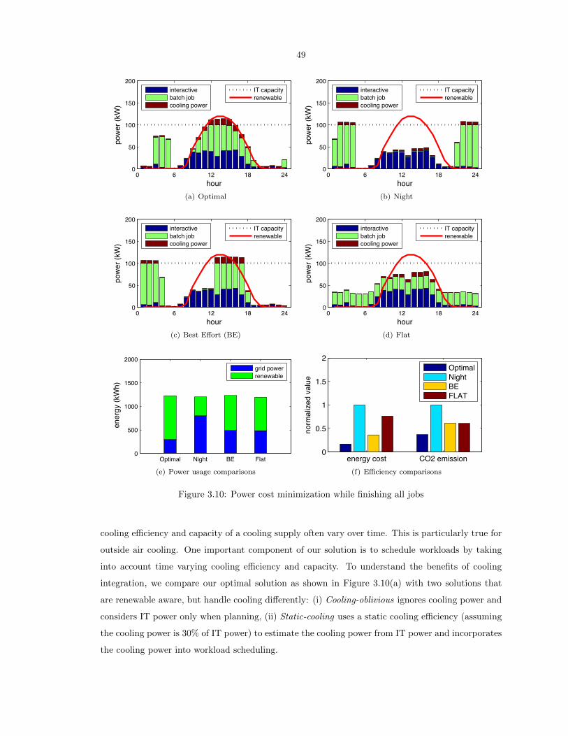
49

0 6 12 18 240

50

100

150

200

hour

powe

r (kW

)

interactivebatch jobcooling power

IT capacityrenewable

(a) Optimal

0 6 12 18 240

50

100

150

200

hour

powe

r (kW

)



(b) Night

0 6 12 18 240

50

100

150

200

hour

powe

r (kW

)



(c) Best Effort (BE)

0 6 12 18 240

50

100

150

200

hourpo

wer (

kW)



(d) Flat

Optimal Night BE Flat0

500

1000

1500

2000

ener

gy (k

Wh)

grid powerrenewable

(e) Power usage comparisons

energy cost CO2 emission0

0.5

1

1.5

2

norm

alize

d va

lue

OptimalNightBEFLAT

(f) Efficiency comparisons

Figure 3.10: Power cost minimization while finishing all jobs

cooling efficiency and capacity of a cooling supply often vary over time. This is particularly true for

outside air cooling. One important component of our solution is to schedule workloads by taking

into account time varying cooling efficiency and capacity. To understand the benefits of cooling

integration, we compare our optimal solution as shown in Figure 3.10(a) with two solutions that

are renewable aware, but handle cooling differently: (i) Cooling-oblivious ignores cooling power and

considers IT power only when planning, (ii) Static-cooling uses a static cooling efficiency (assuming

the cooling power is 30% of IT power) to estimate the cooling power from IT power and incorporates

the cooling power into workload scheduling.

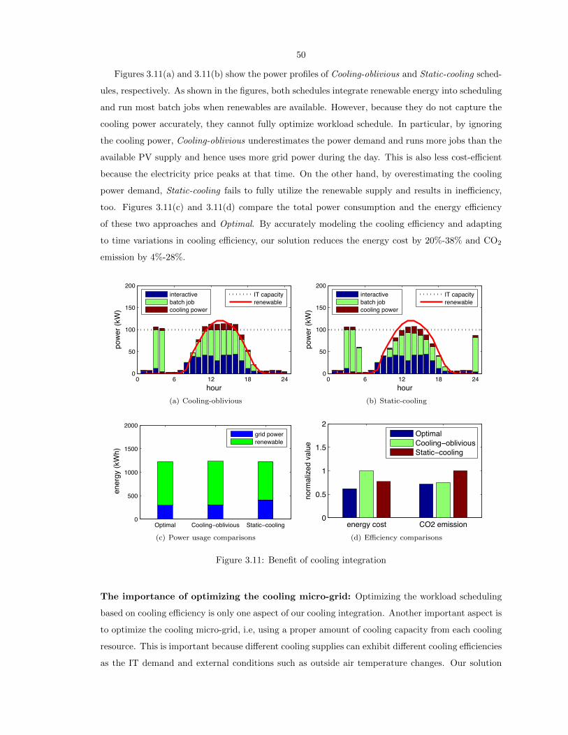
50

Figures 3.11(a) and 3.11(b) show the power profiles of Cooling-oblivious and Static-cooling sched-

ules, respectively. As shown in the figures, both schedules integrate renewable energy into scheduling

and run most batch jobs when renewables are available. However, because they do not capture the

cooling power accurately, they cannot fully optimize workload schedule. In particular, by ignoring

the cooling power, Cooling-oblivious underestimates the power demand and runs more jobs than the

available PV supply and hence uses more grid power during the day. This is also less cost-efficient

because the electricity price peaks at that time. On the other hand, by overestimating the cooling

power demand, Static-cooling fails to fully utilize the renewable supply and results in inefficiency,

too. Figures 3.11(c) and 3.11(d) compare the total power consumption and the energy efficiency

of these two approaches and Optimal. By accurately modeling the cooling efficiency and adapting

to time variations in cooling efficiency, our solution reduces the energy cost by 20%-38% and CO2

emission by 4%-28%.

0 6 12 18 240

50

100

150

200

hour

powe

r (kW

)



(a) Cooling-oblivious

0 6 12 18 240

50

100

150

200

hour

powe

r (kW

)



(b) Static-cooling

Optimal Cooling−oblivious Static−cooling0

500

1000

1500

2000

ener

gy (k

Wh)

grid powerrenewable

(c) Power usage comparisons


0.5

1

1.5

2

norm

alize

d va

lue

OptimalCooling−obliviousStatic−cooling

(d) Efficiency comparisons

Figure 3.11: Benefit of cooling integration

The importance of optimizing the cooling micro-grid: Optimizing the workload scheduling

based on cooling efficiency is only one aspect of our cooling integration. Another important aspect is

to optimize the cooling micro-grid, i.e, using a proper amount of cooling capacity from each cooling

resource. This is important because different cooling supplies can exhibit different cooling efficiencies

as the IT demand and external conditions such as outside air temperature changes. Our solution

51

takes this into account and optimizes the cooling capacity management in addition to IT workload

management.

We compare the following three approaches: (i) Optimal adjusts cooling capacities of outside

air cooling and chiller cooling based on their dynamic cooling efficiencies determined by IT demand

and OAT; (ii) Binary Outside Air (BOA) uses outside air cooling at its full capacity if OAT does

not exceed some threshold (25C) and interactive demand is not too low (less than 10% of the IT

capacity), and use chiller only otherwise; (iii) Chiller only uses the chiller cooling only. All three

solutions are renewable and cooling aware and schedule workload according to the renewable supply

and cooling efficiency. They finish the same number of batch jobs. The difference is how they

manage cooling resources and capacity.

Figure 3.12 shows the cooling capacity from outside air cooling and chiller cooling for these three

solutions. As shown in this figure, Optimal uses outside air only during the night when it is more

efficient, and combines outside air cooling and chiller cooling during other times. In particular, our

solution uses less outside air cooling and more chiller cooling between 12pm and 3pm as outside air

cooling is less efficient due to high IT demand and outside air temperature at that time. In contrast,

BOA runs outside air at full capacity when its efficiency is high and there is enough workload. Chiller

only relies on chiller for all cooling demand. Figures 3.12(g) and 3.12(h) compare the cooling power

and efficiency of the three approaches. By optimizing the cooling substructure, our solution reduces

the cooling power by 66% over BOA and 48% over Chiller only.

Is net-zero energy consumption possible with renewable and cooling aware workload

management?

Now, we switch our goal from minimizing the cost incurred by the data center to minimizing the

environmental impact of the data center. Net-zero is often used to describe a building with zero net

energy consumption and/or emission annually. Recently, researchers have envisioned how net-zero

building concepts can be effectively extended into the data center space to create a net-zero data

center, whose total power consumption does not exceed its total power supply from renewable. We

explore if net-zero is possible with the renewable and cooling aware workload management in data

centers and how much it will cost.

By adding a net-zero constraint (i.e., total power consumption ≤ total renewable supply) to

our optimization problem, our capacity planner can generate a net-zero schedule. Figure 3.13(a)

shows our solution (Net-zero1 ) for achieving a net zero operation goal. Similar to the optimal

solution shown in Figure 3.10(a), Net-zero1 optimally schedules batch jobs to take advantage of the

renewable supply; however, batch jobs are only executed when renewable energy is available and

without exceeding the total renewable generation, and thus some are allowed to not finish during

this 24 hour period. In this case, about 40% of the batch jobs are delayed until a future time when

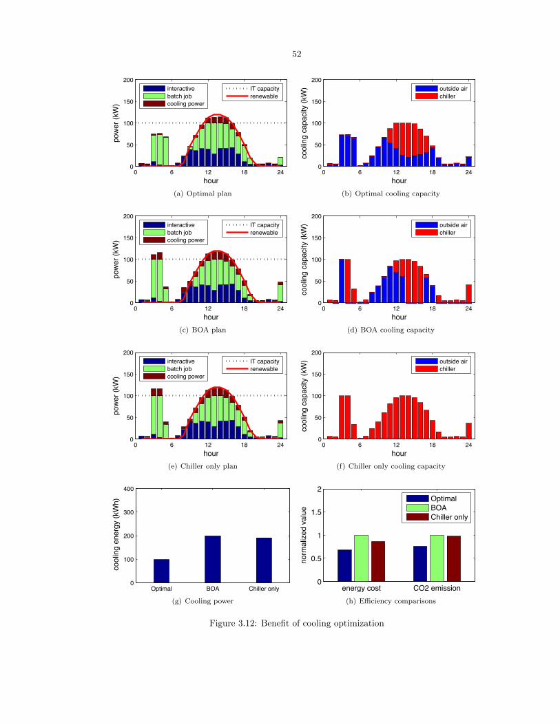
52

0 6 12 18 240

50

100

150

200

hour

powe

r (kW

)



(a) Optimal plan

0 6 12 18 240

50

100

150

200

hour

cool

ing

capa

city

(kW

)

outside airchiller

(b) Optimal cooling capacity

0 6 12 18 240

50

100

150

200

hour

powe

r (kW

)



(c) BOA plan

0 6 12 18 240

50

100

150

200

hourco

olin

g ca

pacit

y (k

W)

outside airchiller

(d) BOA cooling capacity

0 6 12 18 240

50

100

150

200

hour

powe

r (kW

)



(e) Chiller only plan

0 6 12 18 240

50

100

150

200

hour

cool

ing

capa

city

(kW

)

outside airchiller

(f) Chiller only cooling capacity

Optimal BOA Chiller only0

100

200

300

400

cool

ing

ener

gy (k

Wh)

(g) Cooling power


0.5

1

1.5

2

norm

alize

d va

lue

OptimalBOAChiller only

(h) Efficiency comparisons

Figure 3.12: Benefit of cooling optimization

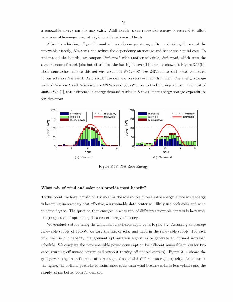
53

a renewable energy surplus may exist. Additionally, some renewable energy is reserved to offset

non-renewable energy used at night for interactive workloads.

A key to achieving off grid beyond net zero is energy storage. By maximizing the use of the

renewable directly, Net-zero1 can reduce the dependency on storage and hence the capital cost. To

understand the benefit, we compare Net-zero1 with another schedule, Net-zero2, which runs the

same number of batch jobs but distributes the batch jobs over 24-hours as shown in Figure 3.13(b).

Both approaches achieve this net-zero goal, but Net-zero2 uses 287% more grid power compared

to our solution Net-zero1. As a result, the demand on storage is much higher. The energy storage

sizes of Net-zero1 and Net-zero2 are 82kWh and 330kWh, respectively. Using an estimated cost of

400$/kWh [7], this difference in energy demand results in $99,200 more energy storage expenditure

for Net-zero2.

0 6 12 18 240

50

100

150

200

hour

powe

r (kW

)



(a) Net-zero1

0 6 12 18 240

50

100

150

200

hour

powe

r (kW

)



(b) Net-zero2

Figure 3.13: Net Zero Energy

What mix of wind and solar can provide most benefit?

To this point, we have focused on PV solar as the sole source of renewable energy. Since wind energy

is becoming increasingly cost-effective, a sustainable data center will likely use both solar and wind

to some degree. The question that emerges is what mix of different renewable sources is best from

the perspective of optimizing data center energy efficiency.

We conduct a study using the wind and solar traces depicted in Figure 3.2. Assuming an average

renewable supply of 100kW, we vary the mix of solar and wind in the renewable supply. For each

mix, we use our capacity management optimization algorithm to generate an optimal workload

schedule. We compare the non-renewable power consumption for different renewable mixes for two

cases (turning off unused servers and without turning off unused servers). Figure 3.14 shows the

grid power usage as a function of percentage of solar with different storage capacity. As shown in

the figure, the optimal portfolio contains more solar than wind because solar is less volatile and the

supply aligns better with IT demand.

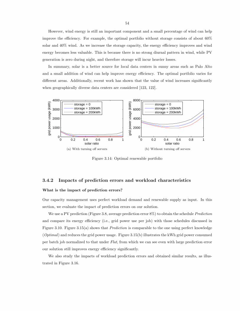
54

However, wind energy is still an important component and a small percentage of wind can help

improve the efficiency. For example, the optimal portfolio without storage consists of about 60%

solar and 40% wind. As we increase the storage capacity, the energy efficiency improves and wind

energy becomes less valuable. This is because there is no strong diurnal pattern in wind, while PV

generation is zero during night, and therefore storage will incur heavier losses.

In summary, solar is a better source for local data centers in sunny areas such as Palo Alto

and a small addition of wind can help improve energy efficiency. The optimal portfolio varies for

different areas. Additionally, recent work has shown that the value of wind increases significantly

when geographically diverse data centers are considered [123, 122].

0 0.2 0.4 0.6 0.8 10

1000

2000

3000

4000

solar ratio

grid

pow

er u

sage

(kW

h)

storage = 0storage = 100kWhstorage = 200kWh

(a) With turning off servers

0 0.2 0.4 0.6 0.8 10

2000

4000

6000

8000

solar ratio

grid

pow

er u

sage

(kW

h)

storage = 0storage = 100kWhstorage = 200kWh

(b) Without turning off servers

Figure 3.14: Optimal renewable portfolio

3.4.2 Impacts of prediction errors and workload characteristics

What is the impact of prediction errors?

Our capacity management uses perfect workload demand and renewable supply as input. In this

section, we evaluate the impact of prediction errors on our solution.

We use a PV prediction (Figure 3.8, average prediction error 8%) to obtain the schedule Prediction

and compare its energy efficiency (i.e., grid power use per job) with those schedules discussed in

Figure 3.10. Figure 3.15(a) shows that Prediction is comparable to the one using perfect knowledge

(Optimal) and reduces the grid power usage. Figure 3.15(b) illustrates the kWh grid power consumed

per batch job normalized to that under Flat, from which we can see even with large prediction error

our solution still improves energy efficiency significantly.

We also study the impacts of workload prediction errors and obtained similar results, as illus-

trated in Figure 3.16.

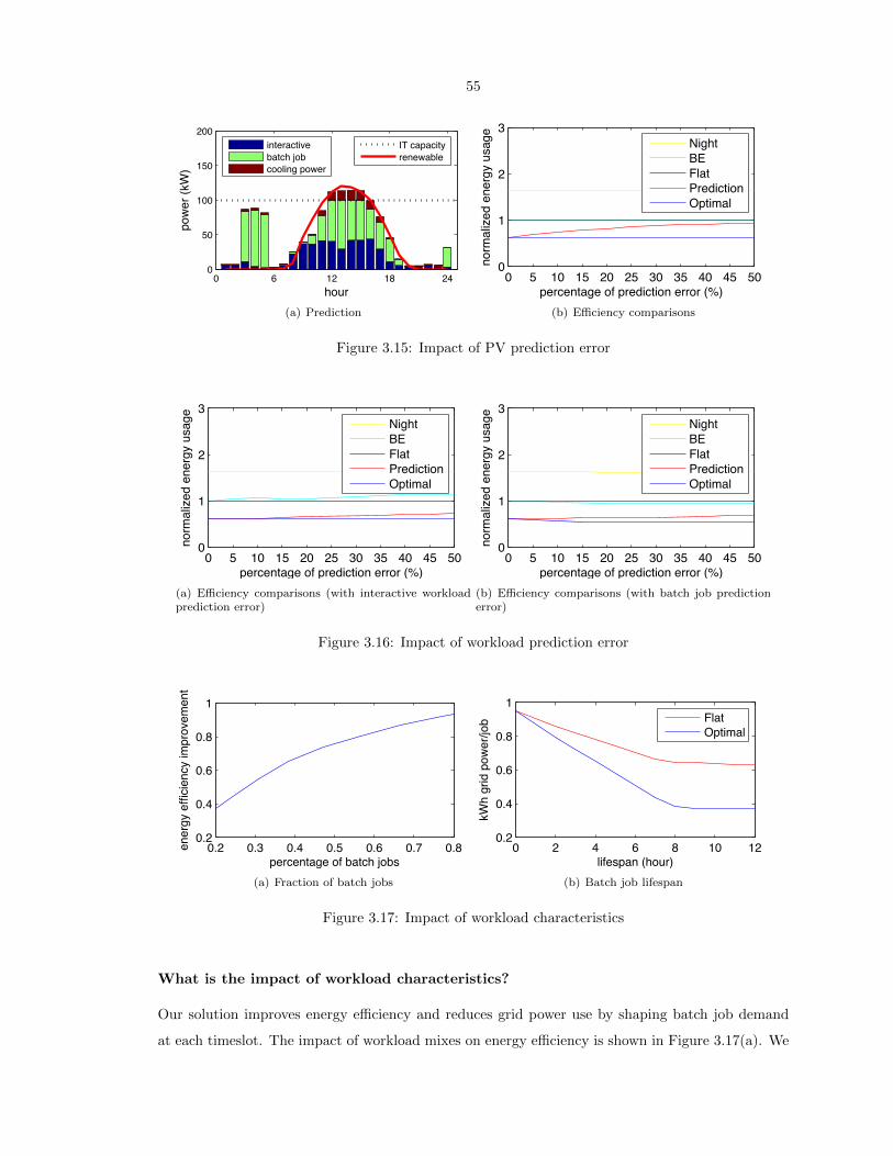
55

0 6 12 18 240

50

100

150

200

hour

powe

r (kW

)



(a) Prediction

0 5 10 15 20 25 30 35 40 45 500

1

2

3

norm

aliz

ed e

nerg

y us

age

percentage of prediction error (%)

NightBEFlatPredictionOptimal

(b) Efficiency comparisons

Figure 3.15: Impact of PV prediction error

0 5 10 15 20 25 30 35 40 45 500

1

2

3

norm

aliz

ed e

nerg

y us

age



(a) Efficiency comparisons (with interactive workloadprediction error)

0 5 10 15 20 25 30 35 40 45 500

1

2

3

norm

aliz

ed e

nerg

y us

age



(b) Efficiency comparisons (with batch job predictionerror)

Figure 3.16: Impact of workload prediction error

0.2 0.3 0.4 0.5 0.6 0.7 0.80.2

0.4

0.6

0.8

1

percentage of batch jobs

ener

gy e

fficie

ncy

impr

ovem

ent

(a) Fraction of batch jobs

0 2 4 6 8 10 120.2

0.4

0.6

0.8

1

lifespan (hour)

kWh

grid

pow

er/jo

b

FlatOptimal

(b) Batch job lifespan

Figure 3.17: Impact of workload characteristics

What is the impact of workload characteristics?

Our solution improves energy efficiency and reduces grid power use by shaping batch job demand

at each timeslot. The impact of workload mixes on energy efficiency is shown in Figure 3.17(a). We

56

can see that energy efficiency improvement of our solution over Flat increases as the ratio of batch

jobs increases. Finally, we study the impact of job life span (i.e., the time between their arrival and

their deadline) on the energy efficiency. We assume there is one class of batch jobs coming every

hour from midnight to noon. The results in Figure 3.17(b) shows the energy efficiency improves

as the lifespan of jobs increases. This is because a longer lifespan provides greater flexibility in job

scheduling and hence better utilizes renewable supply. Again, our solution is always better than

existing solutions.

3.4.3 Experimental Results on a Testbed

The case studies described in the previous section highlight the theoretical benefits of our approach

over existing solutions. To verify our claims and ensure that we have a practical and robust solution,

we experimentally evaluate our prototype implementation on a data center testbed and contrast it

with a current workload management approach.

Experiment Setup

Our testbed consists of four high end servers (each with two 12-core 1.8GHz processors and 64 GB

memory) and the following workloads: one interactive Web application, and 6 batch applications.

Each server is running Scientific Linux. Each workload is running inside a KVM virtual machine.

The interactive application is a single-tier web application running multiple Apache web servers

and batch jobs are sysbench [4] with different resource demands. httperf [98] is used to replay the

workload demand traces in the form of CGI requests, and each request is directed to one of the Web

servers. The PV, cooling data, and interactive workload traces used in the case study are scaled

to the testbed capacity. We measure the power consumption via the server’s built-in management

interfaces, collect CPU consumption through system monitoring and obtain response times of Web

servers from Apache logs.

Experiment Results

We compare two approaches: (i) Optimal is our optimal design, (ii) Night, which runs batch jobs

at night. For each plan, the runtime workload manager dynamically starts the batch jobs, allo-

cates resources to both interactive and batch workloads and turns on/off servers according to the

plan. We compare the predicted power usage in the plan and the actual power consumption in

Figures 3.18(a) and 3.18(b). Figure 3.18(a) shows the optimal plan for the setting described earlier,

while Figure 3.18(b) shows the results of a more complicated setting, where the critical demand

was comprised of seven 3-tier Web applications (RUBiS, an e-Bay-like online auction), and the non-

critical demand was comprised of 24 batch jobs that included scientific computing, animation and

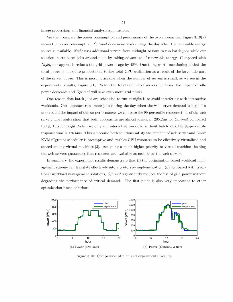
57

image processing, and financial analysis applications.

We then compare the power consumption and performance of the two approaches. Figure 3.19(a)

shows the power consumption. Optimal does more work during the day when the renewable energy

source is available. Night uses additional servers from midnight to 6am to run batch jobs while our

solution starts batch jobs around noon by taking advantage of renewable energy. Compared with

Night, our approach reduces the grid power usage by 48%. One thing worth mentioning is that the

total power is not quite proportional to the total CPU utilization as a result of the large idle part

of the server power. This is most noticeable when the number of servers is small, as we see in the

experimental results, Figure 3.18. When the total number of servers increases, the impact of idle

power decreases and Optimal will save even more grid power.

One reason that batch jobs are scheduled to run at night is to avoid interfering with interactive

workloads. Our approach runs more jobs during the day when the web server demand is high. To

understand the impact of this on performance, we compare the 99-percentile response time of the web

server. The results show that both approaches are almost identical: 205.2ms for Optimal, compared

to 196.1ms for Night. When we only run interactive workload without batch jobs, the 99-percentile

response time is 176.5ms. This is because both solutions satisfy the demand of web server and Linux

KVM/Cgroups scheduler is preemptive and enables CPU resources to be effectively virtualized and

shared among virtual machines [3]. Assigning a much higher priority to virtual machines hosting

the web servers guarantees that resources are available as needed by the web servers.

In summary, the experiment results demonstrate that (i) the optimization-based workload man-

agement scheme can translate effectively into a prototype implementation, (ii) compared with tradi-

tional workload management solutions, Optimal significantly reduces the use of grid power without

degrading the performance of critical demand. The first point is also very important to other

optimization-based solutions.

0 6 12 18 240

200

400

600

800

1000

hour

powe

r (W

att)

planexperiment

(a) Power (Optimal)

0 6 12 18 240

200

400

600

800

1000

1200

1400

hour

pow

er (

Wat

t)

planexperiment

(b) Power (Optimal, 3 tier)

Figure 3.18: Comparison of plan and experimental results

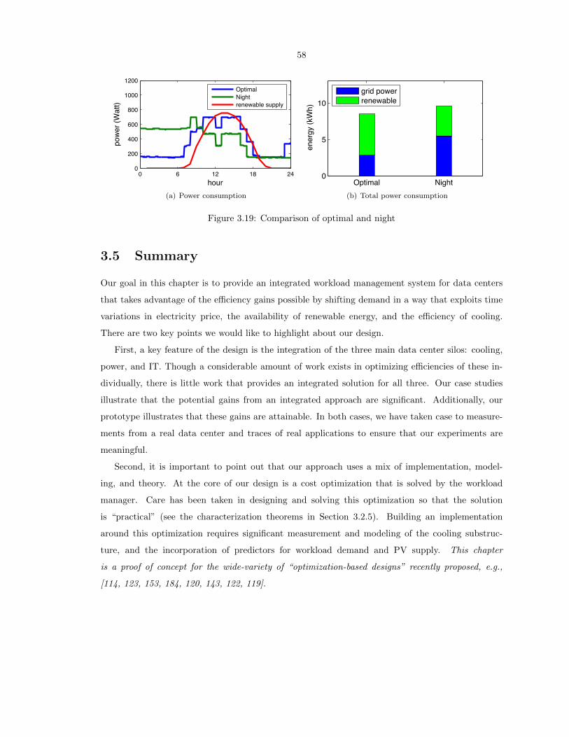
58

0 6 12 18 240

200

400

600

800

1000

1200

hour

powe

r (W

att)

OptimalNightrenewable supply

(a) Power consumption

Optimal Night0

5

10

ener

gy (k

Wh)

grid powerrenewable

(b) Total power consumption

Figure 3.19: Comparison of optimal and night

3.5 Summary

Our goal in this chapter is to provide an integrated workload management system for data centers

that takes advantage of the efficiency gains possible by shifting demand in a way that exploits time

variations in electricity price, the availability of renewable energy, and the efficiency of cooling.

There are two key points we would like to highlight about our design.

First, a key feature of the design is the integration of the three main data center silos: cooling,

power, and IT. Though a considerable amount of work exists in optimizing efficiencies of these in-

dividually, there is little work that provides an integrated solution for all three. Our case studies

illustrate that the potential gains from an integrated approach are significant. Additionally, our

prototype illustrates that these gains are attainable. In both cases, we have taken case to measure-

ments from a real data center and traces of real applications to ensure that our experiments are

meaningful.

Second, it is important to point out that our approach uses a mix of implementation, model-

ing, and theory. At the core of our design is a cost optimization that is solved by the workload

manager. Care has been taken in designing and solving this optimization so that the solution

is “practical” (see the characterization theorems in Section 3.2.5). Building an implementation

around this optimization requires significant measurement and modeling of the cooling substruc-

ture, and the incorporation of predictors for workload demand and PV supply. This chapter

is a proof of concept for the wide-variety of “optimization-based designs” recently proposed, e.g.,

[114, 123, 153, 184, 120, 143, 122, 119].

59

Chapter 4

IT for Sustainability: Data CenterDemand Response

Demand response (DR) programs seek to provide incentives to induce dynamic demand management

of customers’ electricity load in response to power supply conditions, for example, reducing their

power consumption in response to a peak load warning signal or request from the utility. The

National Institute of Standards and Technology (NIST) and the Department of Energy (DoE) have

both identified demand response as one of the priority areas for the future smart grid [140, 57].

In particular, the National Assessment of Demand Response Potential report has identified that

demand response has the potential to reduce up to 20% of the total peak electricity demand across

the country [66]. Further, demand response has the potential to significantly ease the adoption of

renewable energy into the grid.

Data centers represent a particularly promising industry for the adoption of demand response

programs. First, data center energy consumption is large and increasing rapidly. In 2011, data

centers consumed approximately 1.5% of all electricity worldwide, which was about 56% higher than

the preceding five years [79, 78, 160, 110]. Second, data centers are highly automated and monitored,

and so there is the potential for a high-degree of responsiveness. For example, today’s data centers

are well instrumented with a rich set of sensors and actuators. The power load and state of IT

equipment (e.g., server, storage and networking devices) and cooling facility (e.g., CRAC units) can

be continuously monitored and panoramically adjusted. Third, many workloads in data centers are

delay tolerant, and can be scheduled to finish anytime before their deadlines. This enables significant

flexibility for managing power demand. Finally, local power generation, e.g., both traditional backup

generators such as diesel or natural gas powered generators and newer renewable power installations

such as solar PV arrays, can help reduce the need from the grid by supplying the demand at critical

times. In particular, local power generation combined with workload management has a significant

potential to shed the peak load and reduce energy costs.

Despite wide recognition of the potential for demand response in data centers, the current reality

60

is that industry data centers seemingly perform little, if any, demand response [79, 78]. One of

the most common demand response programs available is Coincident Peak Pricing (CPP), which

is required for medium and large industrial consumers in many regions. These programs work by

charging a very high price for usage during the coincident peak hour, often over 200 times higher

than the base rate, where the coincident peak hour is the hour when the most electricity is requested

by the utility from its wholesale electric supplier. It is common for the coincident peak charges to

account for 23% or more of a customer’s electric bill according to Fort Collins Utilities [67]. Hence,

from the perspective of a consumer, it is critical to control and reduce usage during the peak hour.

Although it is impossible to accurately predict exactly when the peak hour will occur, many utilities

identify potential peak hours and send warning signals to customers, which helps customers manage

their loads and make decisions about their energy usage. For example, Fort Collins Utilities sends

coincident peak warnings for 3-22 hours each month with an average 14.5 in summer months and

10 in winter ones. Depending on the utility, warnings may come between 5 minutes and 24 hours

ahead of time.

Coincident peak pricing is not a new phenomenon. In fact, it has been used for large industrial

consumers for decades. However, it is rare for large industrial consumers to have the responsiveness

that data centers can provide. Unfortunately, data centers today either do not respond to coincident

peak warnings or simply respond by turning on their backup power generators [6]. Using backup

power generation seems appealing since it can be automated easily, it does not impact operations, and

it provides demand response for the utility company. However, the traditional backup generators at

data centers can be very “dirty” – in some cases even not meeting Environmental Protection Agency

(EPA) emissions standards [79]. So, from an environmental perspective, this form of response is far

from ideal. Further, running a backup generator can be expensive. Alternatively, providing demand

response via shifting workload can be more cost effective. One of the challenges with workload shift-

ing is that we need to ensure that the Service Level Agreements (SLAs), e.g., completion deadlines,

remain satisfied even with uncertainties in coincident peak and warning patterns, workload demand,

and renewable generation.

Our main contributions are the following. First, we present a detailed characterization study of

coincident peak pricing and provide insight about its properties. Section 4.1 discusses the character-

ization of 26 years’ coincident peak pricing data from Fort Collins Utilities in Colorado. The data

highlights a number of important observations about coincident peak pricing (CPP). For example,

the data set shows that both the coincident peak occurrence and warning occurrence have strong

diurnal patterns that differ considerably during different days of the week and seasons. Further,

the data highlights that coincident peak warnings are highly reliable – only twice did the coincident

peak not occur during a warning hour. Finally, the data on coincident peak warnings highlights

that the frequency of warnings tends to decrease through the month, and that there tend to be less

61

than seven days per month on which warnings occur.

Second, we develop two algorithms for avoiding the coincident peak and reducing the energy

expenditure using workload shifting and local power generation. Though there has been considerable

recent work studying workload planning in data centers, e.g., [70, 44, 120, 82, 46, 86, 177, 132, 197,

188, 193], the uncertainty of the occurrence of the coincident peak hour presents significant new

algorithmic challenges beyond what has been addressed previously. In particular, small errors in

the prediction of workload or renewable generation have only a small effect on the resulting costs of

workload planning; however, errors in the prediction of the coincident peak have a threshold effect

– if you are wrong you pay a large additional cost. This lack of continuity is well known to make

the development of online algorithms considerably more challenging.

Given the challenges associated with the combination of uncertainty about the coincident peak

hour and warning hours, workload demand, and renewable generation, we consider two design goals

when developing algorithms: good performance in the average case and in the worst case. We

develop an algorithm for each goal. For the average case, we present a stochastic optimization based

algorithm given the estimates of the likelihood of a coincident peak or warning during each hour of the

day, and predictions of workload demand and renewable generation. The algorithm provides provable

robustness guarantees in terms of the variance of the prediction errors. For the worst case scenario,

we propose a robust optimization based algorithm that is computationally feasible and simple, and

guarantees that the cost is within a small constant of the optimal cost of an offline algorithm for any

coincident peak and warning patterns, workload demand, and renewable generation prediction error

distributions with bounded variance. Note that a distinguishing feature of our analysis is that we

provide provable bounds on the impact of prediction errors. In prior work on data center capacity

provisioning prediction errors have almost always been studied via simulation, if at all.

The third main contribution of our work is a detailed study and comparison of the potential

cost savings of algorithms via numerical simulations based on real world traces from production

systems. The experimental results in Section 4.4 highlight a number of important observations.

Most importantly, the results highlight that our proposed algorithms provide significant cost and

emission reductions compared to industry practice and provide close to the minimal costs under

real workloads. Further, our experimental results highlight that both local generation and workload

shifting are important for ensuring minimal energy costs and emissions. Specifically, combining

workload shifting with local generation can provide 35-40% reductions of energy costs, and 10-15%

reductions of emissions. We also illustrate that our algorithms are robust to prediction errors.

Related work

While the design of workload planning algorithms for data centers has received considerable attention

in recent years, e.g., [70, 44, 120, 82, 46, 86, 177, 132, 197, 188, 193] and the references therein;

62

demand response for data centers is a relatively new topic. Some of the initial work in the area comes

from Urgaonkar et al. [174], which proposes an approach for providing demand response by using

energy storage to shift peak demand away from high peak periods. This technique complements

other demand response schemes such as workload shifting. Conceptually, using local storage is

similar to the use of local power generation studied in the current chapter. In this chapter, we

consider both the workload shifting and local power generation. The integration of energy storage

to our framework is a topic of our future work. Another recent approach for data center demand

response is Irwin et al. [103], which studies a distributed storage solution for demand response where

compatible storage systems to optimize I/O throughput, data availability, and energy-efficiency as

power varies. Perhaps the most in depth study of data center demand response to this point is

the recent report released by Lawerence Berkeley National Laboratories (LBNL) [78]. This report

summarizes a field study of four data centers and evaluates the potential of different approaches for

providing demand response. Such approaches include adjusting the temperature set point, shutting

down or idling IT equipment and storage, load migration, and adjusting building properties such

as lighting and ventilation. The results show that data centers can provide 10-12% energy usage

savings at the building level with minimal or no impact to data center operations. This report

highlights the potential of demand response and shows that it is feasible for a data center to respond

to signals from utilities, but stops short of providing algorithms to optimize cost in demand response

programs, which is the focus of the current chapter.

4.1 Coincident peak pricing

Most typically, the demand response programs available for data centers today are some form of

coincident peak pricing. In this section, we give an overview of coincident peak pricing programs

and then do a detailed characterization of the coincident peak pricing program run by Fort Collins

Utilities in Colorado, where HP has a data center charged by this company.

4.1.1 An overview of coincident peak pricing

In a coincident peak pricing program, a customer’s monthly electricity bill is made up of four

components: (i) a fixed connection/meter charge, (ii) a usage charge, (iii) a peak demand charge for

usage during the customer’s peak hour, and (iv) a coincident peak demand charge for usage during

the coincident peak (CP) hour, which is the hour during which the utility company’s usage is the

highest. Each of these is described in detail below.

Connection/Meter charge. The connection and meter charges are fixed charges that cover

the maintenance and construction of electric lines as well as services like meter reading and billing.

For medium and large industrial consumers such as data centers, these charges make up a very small

63

fraction of the total power costs.

Usage charge. The usage charge in CPP programs works similarly to the way it does for

residential consumers. The utility specifies the electricity price $p(t)/kWh for each hour. This price

is typically fixed throughout each season, but can also be time-varying. Usually p(t) is on the order

of several cents per kWh.

Peak demand charge. CPP programs also include a peak demand charge in order to incentivize

customers to consume power in a uniform manner, which reduces costs for the utility due to smaller

capacity provisioning. The peak demand charge is typically computed by determining the hour of

the month during which the customer’s electricity use is highest. This usage is then charged at a

rate of $pp/kWh, which is much higher than p(t). It is typically on the order of several dollars per

kWh.

Coincident peak charge. The defining feature of CPP programs is the coincident peak charge.

This charge is similar to the peak charge, but focuses on the peak hour for the utility as a whole from

its wholesale electricity provider (the coincident peak) rather than the peak hour for an individual

consumer. In particular, at the end of each month the peak usage hour for the utility, tcp, is

determined and then all consumers are charged $pcp/kWh for their usage during this hour. This

rate is again at the scale of several dollars per kWh, and can be significantly larger than the peak

demand charging rate pp.

Note that customers cannot know when the coincident peak will occur since it depends on the

behavior of all of the utility’s customers. As a result, to aid customers the utility sends warnings

that particular hours may be the coincident peak hour. Depending on the utility, these warnings

can be anywhere from 5 minutes to 24 hours ahead of time, though they are most often in the 5-10

minute time-frame. These warnings can last multiple hours and can occur anywhere from two to

tens of times during a month. In practice, these warnings are extremely reliable – the coincident

peak almost never occurs outside of a warning hour. This is important since warnings are the only

signal the utility has for achieving responsiveness from customers.

4.1.2 A case study: Fort Collins Utilities Coincident Peak Pricing (CPP)

Program

In order to provide a more detailed understanding of CPP programs, we have obtained data from the

Fort Collins Utilities on the CPP program they run for medium and large industrial and commercial

customers. The data we have obtained covers the operation of the program from January 1986 to

June 2012. It includes the date and hour of the coincident peak each month as well as the date,

hour, and length of each warning period. In the following we focus our study on three aspects: the

rates, the occurrence of the coincident peak, and the occurrence of the warnings.

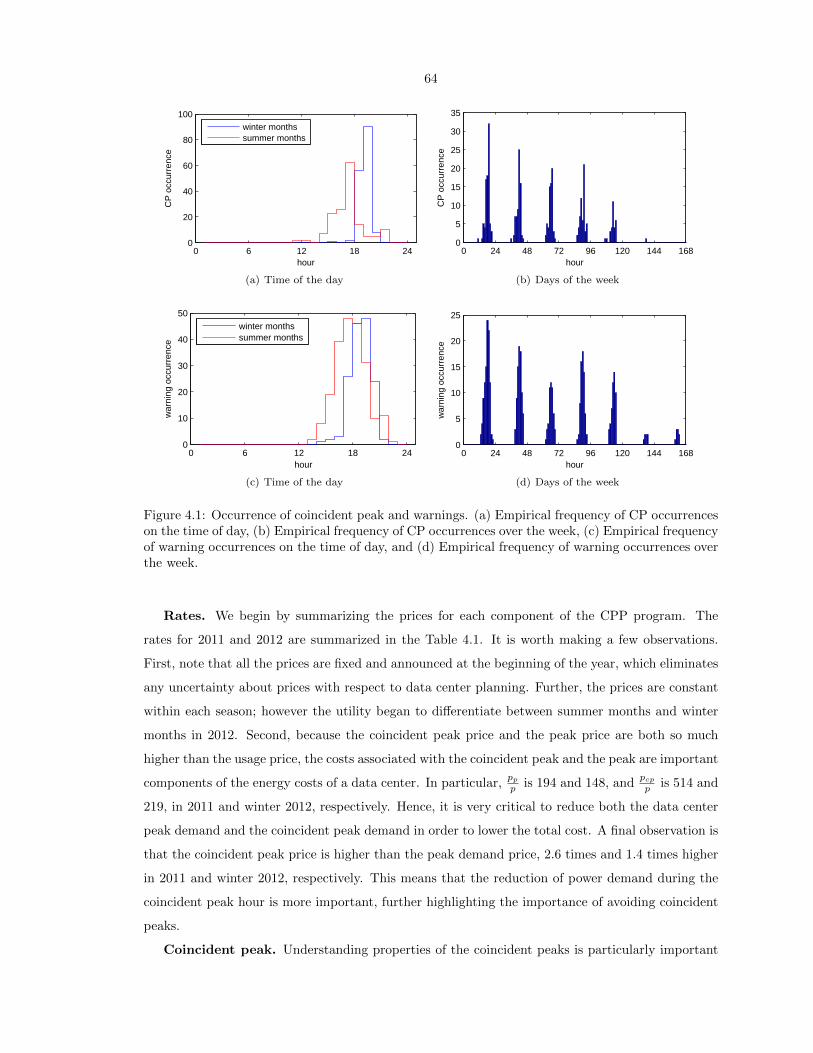
64

0 6 12 18 240

20

40

60

80

100

hour

CP

occ

urre

nce

winter monthssummer months

(a) Time of the day

0 24 48 72 96 120 144 1680

5

10

15

20

25

30

35

hour

CP

occ

urre

nce

(b) Days of the week

0 6 12 18 240

10

20

30

40

50

hour

war

ning

occ

urre

nce

winter monthssummer months

(c) Time of the day

0 24 48 72 96 120 144 1680

5

10

15

20

25

hour

war

ning

occ

urre

nce

(d) Days of the week

Figure 4.1: Occurrence of coincident peak and warnings. (a) Empirical frequency of CP occurrenceson the time of day, (b) Empirical frequency of CP occurrences over the week, (c) Empirical frequencyof warning occurrences on the time of day, and (d) Empirical frequency of warning occurrences overthe week.

Rates. We begin by summarizing the prices for each component of the CPP program. The

rates for 2011 and 2012 are summarized in the Table 4.1. It is worth making a few observations.

First, note that all the prices are fixed and announced at the beginning of the year, which eliminates

any uncertainty about prices with respect to data center planning. Further, the prices are constant

within each season; however the utility began to differentiate between summer months and winter

months in 2012. Second, because the coincident peak price and the peak price are both so much

higher than the usage price, the costs associated with the coincident peak and the peak are important

components of the energy costs of a data center. In particular,ppp is 194 and 148, and

pcpp is 514 and

219, in 2011 and winter 2012, respectively. Hence, it is very critical to reduce both the data center

peak demand and the coincident peak demand in order to lower the total cost. A final observation is

that the coincident peak price is higher than the peak demand price, 2.6 times and 1.4 times higher

in 2011 and winter 2012, respectively. This means that the reduction of power demand during the

coincident peak hour is more important, further highlighting the importance of avoiding coincident

peaks.

Coincident peak. Understanding properties of the coincident peaks is particularly important

65

Charging rates 2011 2012Fixed $/month 54.11 61.96Additional meter $/month 47.81 54.74CP summer $/kWh 12.61 10.20CP winter $/kWh 12.61 7.64Peak $/kWh 4.75 5.44Energy summer $/kWh 0.0245 0.0367Energy winter $/kWh 0.0245 0.0349

Table 4.1: Summary of the charging rates of Fort Collins Utilities during 2011 and 2012 [67].

when considering data center demand response. Figure 4.1 summarizes the coincident peak data we

have obtained from Fort Collins Utilities from January 1986 to June 2012. Figure 4.1(a) depicts the

number of coincident peak occurrences during each hour of the day. From the figure, we can see

that the coincident peak has a strong diurnal pattern: the coincident peak nearly always happens

between 2pm and 10pm. Additionally, the figure highlights that the coincident peak has different

seasonal patterns in winter and summer: the coincident peak occurs later in the day during winter

months than during summer months. Further, the time range that most coincident peaks occur is

narrower during winter months. The number of coincident peak occurrences on a weekly basis is

shown in Figure 4.1(b). The data shows that the coincident peak has a strong weekly pattern: the

coincident peak almost never happens on the weekend, and the likelihood of occurrence decreases

throughout the weekdays.

Warnings. To facilitate customers managing their demand, Fort Collins Utilities identify po-

tential peak hours and send warning signals to customers. These warnings are the key tool through

which utilities achieve responsiveness from customers, i.e., demand response. On average, warnings

from Fort Collins Utilities cover 12 hours for each month. Figures 4.1(c), 4.1(d), and 4.2 summarize

the data on warnings announced by Fort Collins Utilities between January 2010 and June 2012. We

limit our discussion to this period because the algorithm for announcing warnings was consistent

during this interval. During this period, warnings were announced 5-10 minutes before the warning

period began. Note that warnings are only useful if they do in fact align with the coincident peak.

Within our data set, all but two coincident peak fell during a warning period. Further, upon dis-

cussion with the manager of the CPP program, these two mistakes are attributed to human error

rather than an unpredicted coincident peak.

Figure 4.1(c) shows the number of warnings on the time of the day. Given that the warnings are

well correlated with the coincident peak shown in Figure 4.1(a), it is important to understand their

frequency and timing. Unsurprisingly, the announcement of warnings has strong diurnal pattern

similar to that of the coincident peak: most warnings happen between 2pm and 10pm. The seasonal

pattern is also similar to that of the coincident peak: winter months have warnings later in the

day than summer months, and the time range in which most warnings occur is narrower during

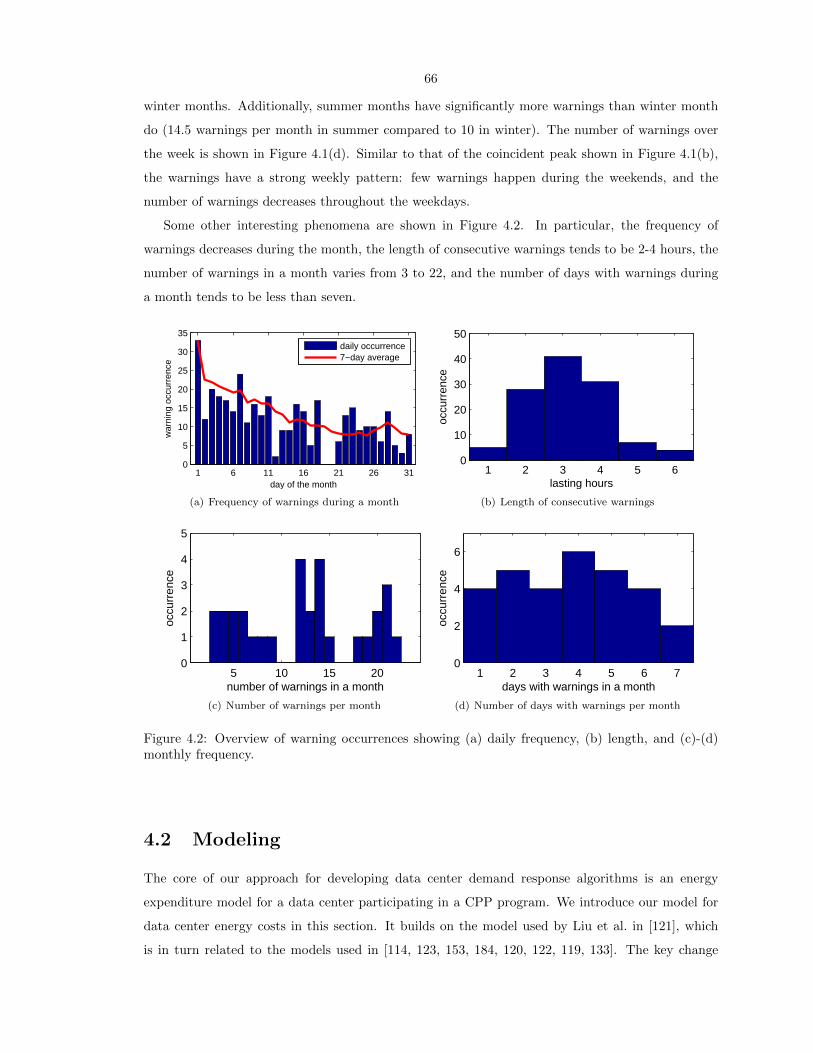
66

winter months. Additionally, summer months have significantly more warnings than winter month

do (14.5 warnings per month in summer compared to 10 in winter). The number of warnings over

the week is shown in Figure 4.1(d). Similar to that of the coincident peak shown in Figure 4.1(b),

the warnings have a strong weekly pattern: few warnings happen during the weekends, and the

number of warnings decreases throughout the weekdays.

Some other interesting phenomena are shown in Figure 4.2. In particular, the frequency of

warnings decreases during the month, the length of consecutive warnings tends to be 2-4 hours, the

number of warnings in a month varies from 3 to 22, and the number of days with warnings during

a month tends to be less than seven.

1 6 11 16 21 26 310

5

10

15

20

25

30

35

day of the month

war

ning

occ

urre

nce

daily occurrence7−day average

(a) Frequency of warnings during a month

1 2 3 4 5 60

10

20

30

40

50

lasting hours

occu

rren

ce

(b) Length of consecutive warnings

5 10 15 200

1

2

3

4

5

number of warnings in a month

occu

rren

ce

(c) Number of warnings per month

1 2 3 4 5 6 70

2

4

6

days with warnings in a month

occu

rren

ce

(d) Number of days with warnings per month

Figure 4.2: Overview of warning occurrences showing (a) daily frequency, (b) length, and (c)-(d)monthly frequency.

4.2 Modeling

The core of our approach for developing data center demand response algorithms is an energy

expenditure model for a data center participating in a CPP program. We introduce our model for

data center energy costs in this section. It builds on the model used by Liu et al. in [121], which

is in turn related to the models used in [114, 123, 153, 184, 120, 122, 119, 133]. The key change

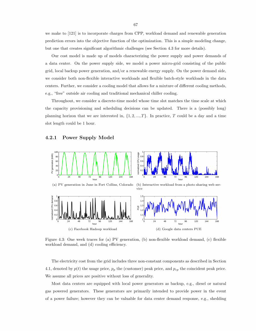
67

we make to [121] is to incorporate charges from CPP, workload demand and renewable generation

prediction errors into the objective function of the optimization. This is a simple modeling change,

but one that creates significant algorithmic challenges (see Section 4.3 for more details).

Our cost model is made up of models characterizing the power supply and power demands of

a data center. On the power supply side, we model a power micro-grid consisting of the public

grid, local backup power generation, and/or a renewable energy supply. On the power demand side,

we consider both non-flexible interactive workloads and flexible batch-style workloads in the data

centers. Further, we consider a cooling model that allows for a mixture of different cooling methods,

e.g., “free” outside air cooling and traditional mechanical chiller cooling.

Throughout, we consider a discrete-time model whose time slot matches the time scale at which

the capacity provisioning and scheduling decisions can be updated. There is a (possibly long)

planning horizon that we are interested in, 1, 2, ..., T. In practice, T could be a day and a time

slot length could be 1 hour.

4.2.1 Power Supply Model

0 24 48 72 96 120 144 1680

20

40

60

80

100

hour

PV

gen

erat

ion

(kW

h)

(a) PV generation in June in Fort Collins, Colorado

0 24 48 72 96 120 144 1680

0.2

0.4

0.6

0.8

1

hour

norm

aliz

ed C

PU

usa

ge

(b) Interactive workload from a photo sharing web ser-vice

0 24 48 72 96 120 144 1680

0.2

0.4

0.6

0.8

1

hour

norm

aliz

ed C

PU

dem

and

(c) Facebook Hadoop workload

0 24 48 72 96 120 144 1681

1.1

1.2

1.3

1.4

1.5

hour

PU

E

(d) Google data centers PUE

Figure 4.3: One week traces for (a) PV generation, (b) non-flexible workload demand, (c) flexibleworkload demand, and (d) cooling efficiency.

The electricity cost from the grid includes three non-constant components as described in Section

4.1, denoted by p(t) the usage price, pp the (customer) peak price, and pcp the coincident peak price.

We assume all prices are positive without loss of generality.

Most data centers are equipped with local power generators as backup, e.g., diesel or natural

gas powered generators. These generators are primarily intended to provide power in the event

of a power failure; however they can be valuable for data center demand response, e.g., shedding

68

peak load by powering the data center with local generation. Typically, the costs of operating these

generators are dominated by the cost of fuel, e.g., diesel or natural gas. Note that the effective

output of such generators can often be adjusted. In many cases the backup generation is provided

by multiple generators which can be operated independently [22], and in other cases the generators

themselves can be adjusted continuously, e.g., in the case of a GE gas engine [187].

To model such local generators, we assume that the generator has the capacity to power the

whole data center, which is quite common in industry [22], i.e., the total capacity of local generators

Cg = C, where C is the total data center power capacity. We denote the cost in dollar of generating

1kWh power using backup generator by pg. Finally, we denote the generation provided by the local

generator at time t by g(t).

In addition to local backup generators, data centers today increasingly have some form of local

renewable energy available such as PV [93]. The effective output of this type of generation is not

controllable and is often closely tied to external conditions (e.g., wind speed and solar irradiance).

Figure 5.3(a) shows the power generated from a 100kW PV installation in June in Fort Collins,

Colorado. The fluctuation and variability present a significant challenge for data center management.

In this chapter, we consider both data centers with and without local renewable generation. To model

this, we use r(t) to denote the actual renewable energy available to the data center at time t and use

r(t) for the predicted generation. We denote r(t) = (1+ εr)r(t), where εr is the prediction error. We

assume unbiased prediction E [εr] = 0 and denote the variance V [εr] by σ2r , which can be obtained

from historic data. These are standard assumptions in statistics. Let ξr denote the distribution of

εr. In the model, we ignore all fixed costs associated with local generation, e,g., capital expenditure

and renewable operational and maintenance cost.

4.2.2 Power Demand Model

The power demand model is derived from models of the workload and the cooling demands of the

data center.

Workload model. Most data centers support a range of IT workloads, including both non-

flexible interactive applications that run 24x7 (such as Internet services, online gaming) and delay

tolerant, flexible batch-style applications (e.g., scientific applications, financial analysis, and image

processing). Flexible workloads can be scheduled to run anytime as long as the jobs finish before

their deadlines. These deadlines are much more flexible (several hours to multiple days) than that

of interactive workload. The prevalence of flexible workloads provides opportunities for providing

demand response via workload shifting/shaping.

We assume that there are I interactive workloads. For interactive workload i, the arrival rate

at time t is λi(t). Then based on the service rate and the target performance metrics (e.g., average

delay, or 95th percentile delay) specified in SLAs, we can obtain the IT capacity required to allocate

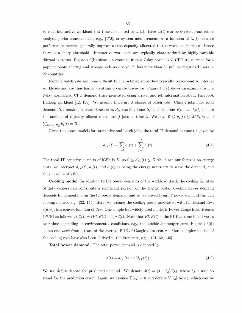
69

to each interactive workload i at time t, denoted by ai(t). Here ai(t) can be derived from either

analytic performance models, e.g., [172], or system measurements as a function of λi(t) because

performance metrics generally improve as the capacity allocated to the workload increases, hence

there is a sharp threshold. Interactive workloads are typically characterized by highly variable

diurnal patterns. Figure 4.3(b) shows an example from a 7-day normalized CPU usage trace for a

popular photo sharing and storage web service which has more than 85 million registered users in

22 countries.

Flexible batch jobs are more difficult to characterize since they typically correspond to internal

workloads and are thus harder to attain accurate traces for. Figure 4.3(c) shows an example from a

7-day normalized CPU demand trace generated using arrival and job information about Facebook

Hadoop workload [42, 196]. We assume there are J classes of batch jobs. Class j jobs have total

demand Bj , maximum parallelization MPj , starting time Sj and deadline Ej . Let bj(t) denote

the amount of capacity allocated to class j jobs at time t. We have 0 ≤ bj(t) ≤ MPj ,∀t and∑t∈[Sj ,Ej ]

bj(t) = Bj .

Given the above models for interactive and batch jobs, the total IT demand at time t is given by

dIT (t) =

I∑i=1

ai(t) +

J∑j=1

bj(t). (4.1)

The total IT capacity in units of kWh is D, so 0 ≤ dIT (t) ≤ D,∀t. Since our focus is on energy

costs, we interpret dIT (t), ai(t), and bj(t) as being the energy necessary to serve the demand, and

thus in units of kWh.

Cooling model. In addition to the power demands of the workload itself, the cooling facilities

of data centers can contribute a significant portion of the energy costs. Cooling power demand

depends fundamentally on the IT power demand, and so is derived from IT power demand through

cooling models, e.g., [32, 145]. Here, we assume the cooling power associated with IT demand dIT ,

c(dIT ), is a convex function of dIT . One simple but widely used model is Power Usage Effectiveness

(PUE) as follows: c(d(t)) = (PUE(t)− 1)∗d(t). Note that PUE(t) is the PUE at time t, and varies

over time depending on environmental conditions, e.g., the outside air temperature. Figure 4.3(d)

shows one week from a trace of the average PUE of Google data centers. More complex models of

the cooling cost have also been derived in the literature, e.g., [121, 32, 145].

Total power demand. The total power demand is denoted by

d(t) = dIT (t) + c(dIT (t)). (4.2)

We use d(t)to denote the predicted demand. We denote d(t) = (1 + εd)d(t), where εd is used to

stand for the prediction error. Again, we assume E [εd] = 0 and denote V [εd] by σ2d, which can be

70

obtained from historic data. Let ξd denote the distribution of εd.

4.2.3 Total data center costs

Using the above models for the power supply and power demand at a data center, we can now model

the operational energy cost of a data center, which our data center demand response algorithms seek

to minimize. In particular, they take the power supply cost parameters, including the grid power

pricing and fuel cost, as well as the workload demand and SLAs information, as input and seek to

provide an near-optimal workload schedule and a local power generation plan given uncertainties

about workload demand and renewable generation. This planning problem can be formulated as the

following constrained convex optimization problem given tcp.

minb,g

T∑t=1

p(t)e(t) + ppmaxte(t) + pcpe(tcp) + pg

T∑t=1

g(t) (4.3a)

s.t. e(t) ≡ (d(t)− r(t)− g(t))+ ≤ C, ∀t (4.3b)∑t∈[Sj ,Ej ]

bj(t) = Bj , ∀j (4.3c)

0 ≤ bj(t) ≤MPj , ∀j,∀t (4.3d)

0 ≤ dIT (t) ≤ D, ∀t (4.3e)

0 ≤ g(t) ≤ Cg. ∀t (4.3f)

In the above optimization, the objective (4.3a) captures the operational energy cost of a data

center, including the electricity charge by the utility and the fuel cost of using local power generation.

The first three terms describe grid power usage charge, peak demand charge, and coincident peak

charge, respectively. The fuel cost of the local power generator is specified in the last term. Further,

the first constraint (4.3b) defines e(t) to be the power consumption from the grid at time t, which

depends on the IT demand dIT (t) defined in (4.1) and therefore further depends on batch job

scheduling bj(t), the cooling demand, the availability of renewable energy, and the use of the local

backup generator. Constraint (4.3c) requires all jobs to be completed. Constraint (4.3d) limits the

parallelism of the batch jobs. Constraint (4.3e) limits the demand served in each time slot by the

IT capacity of the data center. The final constraint (4.3f) limits the capacity of the local generation.

4.3 Algorithms

We now present our algorithms for workload and generation planning in data centers that partic-

ipate in CPP programs. In particular, our starting point is the data center optimization problem

introduced in (4.3a) in the previous section, and our goal is to design algorithms for optimally

71

combining local generation and workload shifting in order to minimize the operational energy cost.

More specifically, the algorithmic problem we approach is as follows. We assume that the planning

horizon being considered is one day and that the workload, prices, cooling efficiency, and renewable

availability can be predicted with reasonable accuracy in this horizon, but that the planner does

not know when the coincident peak and the corresponding warnings will occur. The algorithmic

goal is thus to generate a plan that minimizes cost despite this unknown information and prediction

errors. Since the costs associated with the coincident peak can be a large fraction of the data center

electricity bill, this lack of information is a significant challenge for planning. As we have already

discussed, designing for this uncertainty about the coincident peak is fundamentally different than

designing for prediction errors on factors such as workload demand or renewable generation since

inaccuracies in the prediction of the coincident peak and the corresponding warnings have a discon-

tinuous threshold effect on the realized cost. As a result, even small prediction errors can result in

significantly increased costs. Such effects are well-known to make the design of online algorithms

difficult.

We consider two approaches for handling uncertainty about the coincident peak. The first ap-

proach we follow is to estimate when the coincident peak and the corresponding warnings will occur.

Using the estimated likelihood of a warning and/or coincident peak during each hour, we can for-

mulate a convex optimization problem to minimize the expected cost in the planning horizon. The

second approach we follow is to formulate a robust optimization that seeks to minimize the worst

case cost given adversarial placement of warnings and the coincident peak. Note that throughout

this chapter we restrict our attention to algorithms that do “non-adaptive” workload shifting, i.e.,

algorithms that plan workload shifting once at the beginning of the horizon and then do not adjust

the plan during the horizon in order to make them more easily adoptable. However, we do allow local

generation to be turned on adaptively when warnings are received. This restriction is motivated by

industry practice today – adaptive workload shifting for demand response is nearly non-existent, but

data centers that actively participate in demand response programs do adjust local generation when

warnings are received. This restriction can easily be relaxed in what follows.1 However, the fact that

our analytic results provide guarantees for non-adaptive workload planning means they are stronger.

Further, our numerical experiments studying the improvements from adaptive workload planning

(omitted due to space restrictions) highlight that the benefit of such adaptivity is not large. This

can be seen already in our results since the gap between the costs of our non-adaptive algorithms

and the cost of the offline optimal is small.

1If it is relaxed, replanning after warnings occur can be beneficial. Interestingly, such replanning could have similarand only slightly better performance in the worst case. We omit the results due to space consideration.

72

4.3.1 Expected cost optimization

The starting point for our algorithms is the data center optimization in (4.3a). In this section, our

goal is to plan workload allocation and local generation in order to minimize the expected cost of

the data center given estimates from historical data about when the warnings and the coincident

peak will occur. In particular, our approach uses historical data about when warnings will occur in

order to estimate the likelihood that time slot t will be a warning. We denote the estimate at time

t by w(t), and the full estimator by W.

Since the data center has local backup generation, it can provide demand response even without

using adaptive workload shifting by turning on the backup generator when warnings are received

from the utility. Today, those data centers that actively participate in demand response programs

typically use this approach. The reason is that the cost of local generation is typically significantly

less than the coincident peak price, and the number of warnings per month is small enough to ensure

that it is cost efficient to always turn on generation whenever warnings are given. Of course, there

are drawbacks to using local generation, since it is typically provided by diesel generators, which

often have very high emissions and costs [61, 79]. Thus, it is important to do workload shifting in a

manner that minimizes the use of local generation, if possible.

Before stating the algorithm formally, let’s briefly discuss its structure. Using the estimates

of warning occurrences, workload demand and renewable generation, we first solve a stochastic

optimization (given in Algorithm 4 below) to obtain a workload schedule b(t) and local generator

usage plan g1(t). Then, in runtime, when the prediction error is harmful, i.e., when

mine(t), εdd(t)− εr r(t) > 0, (4.4)

use the backup generator to remove this effect, i.e., use generation gε(t) = max0,min(e(t), εdd(t)−

εr r(t).2 Additionally, if a warning occurs, turn on the local generator to reduce the demand from

the grid to zero, which we denote by g2(t) = e(t)−gε(t) when t is a warning period in order to ensure

that the coincident peak payment is zero. (Recall that the coincident peak happens within a warning

period with near certainty.) The total local generation used is thus g(t) = g1(t) + gε(t) + g2(t),∀t.

More formally, to write the objective function used for the first step of planning we first need to

estimate g2(t), which can be done as follows:

g2(t) =

e(t)− gε(t) if t is a warning hour

0 otherwise

This is feasible since in practice the generator has the capacity to power the whole data center [22],

i.e., Cg = C.

73

We can now formally define the planning algorithm for expected cost minimization. Define e(t) ≡(d(t)− r(t)− g1(t)

)+

as the predicted power demand from utility at time t, and σ ≡maxσd, σr

as a upper bound of normalized variance of the power demand from utility.

Algorithm 4. Estimate w(t) for all t in the planning period. Then, solve the following convex

optimization:

minb,g1

T∑t=1

((1− w(t))p(t) + w(t)pg) e(t) + ppmaxte(t) + pg

T∑t=1

g1(t) (4.5a)

s.t. e(t) ≡(d(t)− r(t)− g1(t)

)+

≤ C, ∀t (4.5b)∑t∈[Sj ,Ej ]

bj(t) = Bj , ∀j (4.5c)

0 ≤ bj(t) ≤MPj , ∀j,∀t (4.5d)

0 ≤ d(t) ≤ D, ∀t (4.5e)

0 ≤ g1(t) ≤ Cg. ∀t (4.5f)

During operation, if the prediction error has negative effect satisfying (4.4), use backup generation

to remove the error.2 If a warning is received, use the local generator to reduce the power usage from

the grid to zero until the warning period ends.

Of course there are many approaches for estimating w(t) in practice. In this chapter, we do this

using the historical data summarized in Section 4.1. Since our data is rich, and the occurrence of

the warnings is fairly stationary, this estimator is accurate enough to achieve good performance, as

we show in Section 4.4. Of course, in practice, predictions could likely be improved by incorporating

information such as weather predictions.

It is clear that the performance of Algorithm 4 is highly dependent on the accuracy of predictions,

thus it is important to characterize this dependence. To accomplish this, denote the objective

function in (4.3a) by f(b,g). Then the expected cost of Algorithm 4 is Eξd,ξr,W [f(bs,gs)]. We

compare this cost to the expected cost of oracle-like offline algorithm that knows workload demand

and renewable generation perfectly, which we denote by Eξd,ξr,W [f(b∗,g∗)]. To characterize the

performance of the algorithm we use the competitive ratio, which is defined as the ratio of the cost

of a given algorithm to the cost of the offline optimal algorithm. The following theorem (proven in

Appendix C.1) shows that the cost of the online algorithm is not too much larger than optimal as

long as predictions are accurate.

2Note that, in practice, one would not want to use generation to correct for all prediction errors, such a correctionwould only be done if the prediction error was extreme. However, for analytic simplification, we assume that allprediction errors are erased in this manner and evaluate the resulting cost. Our simulations results in Section 4.4 usethe generator only to correct for extreme prediction errors.

74

Theorem 12. Given that the standard deviation of prediction errors for the workload and renewable

generation are bounded by σ and the distribution of coincident peak warnings is known precisely,

Algorithm 4 has a competitive ratio of 1 +Bσ, where B =pgΣt(d

s(t)+r(t))2Eεd [f∗(e∗,g∗)] +

pgΣt(d∗(t)+r(t))

2Eεd [f∗(e∗,g∗)] . That is,

Eξd,ξr,W [f(bs,gs)] /Eξd,ξr,W [f(b∗,g∗)] ≤ 1 +Bσ.

It is worth noting that it is rare for the impact of prediction error on a data center planning

algorithm to be quantified analytically, nearly all prior work either does not study the impact of

prediction errors, or studies their impact via simulation only. Additionally, it is important to point

out that Theorem 12 does not make any distributional assumption on the prediction errors other

than bounded variance. The key observation provided by Theorem 12 is that the competitive ratio

is a linear function of prediction standard deviation, which implies when prediction errors decrease

to 0, this competitive ratio also decreases to 1. Thus, the algorithm is fairly robust to prediction

errors. Our trace-based simulations in Section 4.4 corroborate this conclusion.

4.3.2 Robust optimization

While performing well for expected cost is a natural goal, the algorithm we have discussed above

depends on the accuracy of estimators of the occurrence of the coincident peak or warning periods.

In this section, we focus on providing algorithms that maintain worst-case guarantees regardless of

prediction accuracy, i.e., that minimize the worst case cost. To characterize the performance of the

algorithm we again use the competitive ratio. In our setting, we consider the cost only during one

planning period. Thus, the difference in information between the offline algorithm and our algorithm

is knowledge of when the warnings will occur, exact workload demand and renewable generation.

We do assume that the online algorithm has an upper bound on the number of warnings that may

occur.

In order to minimize the worst case cost, the natural approach is to increase the penalty on the

peak period. This follows because, if an adversary seeks to maximize the cost of an algorithm, it

should place warnings on the periods where the algorithm uses the most energy. This observation

leads us to the following algorithm:

Algorithm 5. Consider an upper bound on the number of warning periods W . Solve the following

75

convex optimization

minb,g1

T∑t=1

p(t)e(t) +(pp + W (pg −mintp(t))

)maxte(t) + pg

T∑t=1

g1(t) (4.6a)

s.t. e(t) ≡(d(t)− r(t)− g1(t)

)+

≤ C, ∀t (4.6b)∑t∈[Sj ,Ej ]

bj(t) = Bj , ∀j (4.6c)

0 ≤ bj(t) ≤MPj , ∀j,∀t (4.6d)

0 ≤ d(t) ≤ D, ∀t (4.6e)

0 ≤ g1(t) ≤ Cg. ∀t (4.6f)

During operation, if the prediction error has negative effect satisfying (4.4), use backup generation

to remove the error.2 If a warning is received, use the local generator to reduce the power usage from

the grid to zero until the warning period ends.

This algorithm represents a seemingly easy change to the original data center optimization in

(4.3a); however the subtle differences are enough to ensure that it provide a very strong worst case

cost guarantee. In particular, it provides the minimal competitive ratio achievable as stated in the

following theorem, which is proven in Appendix C.1.

Theorem 13. Given that the standard deviation of prediction errors for the workload and renewable

generation are bounded by σ, Algorithm 5 has a competitive ratio of

1 +Bσ +W (pg −mintp(t))

Tmintp(t)/PMR∗ + pp≤ 1 +Bσ +

W (pg −mintp(t))

pp,

where B =pgΣt(d

w(t)+r(t))2Eεd [f∗(e∗,g∗)] +

pgΣt(d∗(t)+r(t))

2Eεd [f∗(e∗,g∗)] . Further, if W = |W | then there is a lower bound

1 +W (pg−mintp(t))

Tmintp(t)/PMR∗+ppon the competitive ratio achievable under any online algorithm, even one

with exact predictions of workloads and renewable generation.

The key contrast between Theorem 13 and Theorem 12 is that Theorem 12 assumes that the

distribution of coincident peak warnings is known precisely, while Theorem 13 provides a bound even

when the coincident peak warnings are adversarial. As such, it is not surprising that the competitive

ratio is larger in Theorem 13. However, note that the competitive ratio of Algorithm 4 in the context

of Theorem 13 can be easily shown to be unbounded, and so one should not think of Theorem 12

as a stronger bound than Theorem 13.

Interestingly, the form of Theorem 13 parallels Theorem 12, except with an additional term in

competitive ratio. Thus, again the competitive ratio grows linearly with the variance of the prediction

error. Additionally, note that when σ = 0, the competitive ratio matches the lower bound, which

76

highlights that the additional term in Theorem 13 is tight. Further, since the additional term is

defined in terms of the relative prices of local generation and the peak, it is easy to understand its

impact in practice. In practice, pg is less than $0.3/kWh [157] and the number of warning hours is

roughly between 3 and 22, with an average of 12 warning hours per month. So, this term is typically

less than 1, which highlights that the worst-case bound on Algorithm 5 nearly matches the bound

on Algorithm 4 in the case where the coincident peak warning distribution is known.

Note that, if there is no local generator, then we can derive a similar result to Theorem 13, where

W (pg −mintp(t)) is replaced by pcp. The comparison of these results highlights the cost savings

provided by using a local backup generator. Since the data center does not know the exact number

of warnings for a particular month, whether or not using local generation is beneficial depends on

the predicted bound on the number of warnings per month. If it is smaller than⌊

pcppg−mintp(t)

⌋(25 in

winter and 36 in summer for 2012 in the utility scheme shown in Table 4.1 with high local generation

cost), it should use local generation. This highlights that if a utility wishes to incentivize the data

center to use local generation to relieve its pressure, then it should not send too many warnings.

4.3.3 Implementation considerations

Over the past decade there has been significant effort to address data center energy challenges via

workload management. Most of these efforts focus on improving the energy efficiency and achieving

energy proportionality of data centers via workload consolidation and dynamic capacity provisioning,

e.g., [70, 44, 120, 82, 46, 86, 177, 132, 197, 188, 193]. Recently, such work has begun to explore

topics such as shifting (temporal) or migrating (spatial) workloads to better use renewable energy

sources [150, 123, 122, 166, 112, 119, 81, 53].

The algorithms presented in this section are both optimization-based approaches for temporal

workload management and, as such, build on this literature. In particular, optimization based

approaches have received significant attention in recent years, and have been shown to transition

easily to large scale implementations, e.g., [121, 70, 78]. In this chapter, we evaluate the algorithms

presented above via both worst-case analysis and trace-based simulations. However, for completeness

we comment briefly here on the important considerations for implementation of these designs. For

more details, the reader should consult [121, 70, 78]. Implementation considerations typically fall

into two categories: (i) obtaining accurate predictions of workload, renewable generation, costs,

etc.; (ii) implementing the plan generated by the algorithm. Each of these challenges has been well

studied by prior literature, and we only provide a brief description of each in the following.

Predictions. Our algorithms exploit the statistical properties of the coincident peak as well

as predictions of IT demand, cooling costs, renewable generation, etc. Historical data about the

coincident peak is generally available, for large industrial consumers, from the utilities operating

demand response programs. In practice, coincident peak predictions can also be improved using

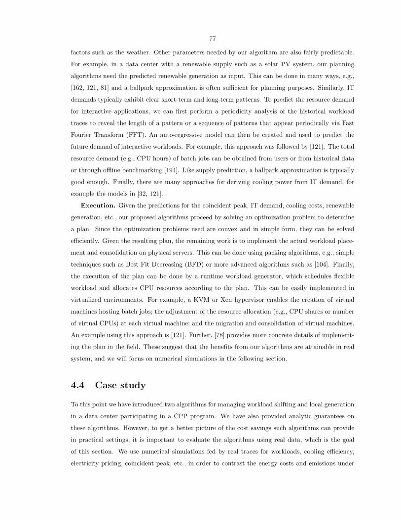
77

factors such as the weather. Other parameters needed by our algorithm are also fairly predictable.

For example, in a data center with a renewable supply such as a solar PV system, our planning

algorithms need the predicted renewable generation as input. This can be done in many ways, e.g.,

[162, 121, 81] and a ballpark approximation is often sufficient for planning purposes. Similarly, IT

demands typically exhibit clear short-term and long-term patterns. To predict the resource demand

for interactive applications, we can first perform a periodicity analysis of the historical workload

traces to reveal the length of a pattern or a sequence of patterns that appear periodically via Fast

Fourier Transform (FFT). An auto-regressive model can then be created and used to predict the

future demand of interactive workloads. For example, this approach was followed by [121]. The total

resource demand (e.g., CPU hours) of batch jobs can be obtained from users or from historical data

or through offline benchmarking [194]. Like supply prediction, a ballpark approximation is typically

good enough. Finally, there are many approaches for deriving cooling power from IT demand, for

example the models in [32, 121].

Execution. Given the predictions for the coincident peak, IT demand, cooling costs, renewable

generation, etc., our proposed algorithms proceed by solving an optimization problem to determine

a plan. Since the optimization problems used are convex and in simple form, they can be solved

efficiently. Given the resulting plan, the remaining work is to implement the actual workload place-

ment and consolidation on physical servers. This can be done using packing algorithms, e.g., simple

techniques such as Best Fit Decreasing (BFD) or more advanced algorithms such as [104]. Finally,

the execution of the plan can be done by a runtime workload generator, which schedules flexible

workload and allocates CPU resources according to the plan. This can be easily implemented in

virtualized environments. For example, a KVM or Xen hypervisor enables the creation of virtual

machines hosting batch jobs; the adjustment of the resource allocation (e.g., CPU shares or number

of virtual CPUs) at each virtual machine; and the migration and consolidation of virtual machines.

An example using this approach is [121]. Further, [78] provides more concrete details of implement-

ing the plan in the field. These suggest that the benefits from our algorithms are attainable in real

system, and we will focus on numerical simulations in the following section.

4.4 Case study

To this point we have introduced two algorithms for managing workload shifting and local generation

in a data center participating in a CPP program. We have also provided analytic guarantees on

these algorithms. However, to get a better picture of the cost savings such algorithms can provide

in practical settings, it is important to evaluate the algorithms using real data, which is the goal

of this section. We use numerical simulations fed by real traces for workloads, cooling efficiency,

electricity pricing, coincident peak, etc., in order to contrast the energy costs and emissions under

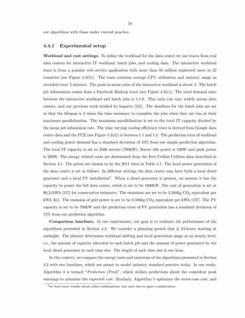
78

our algorithms with those under current practice.


Workload and cost settings. To define the workload for the data center we use traces from real

data centers for interactive IT workload, batch jobs, and cooling data. The interactive workload

trace is from a popular web service application with more than 85 million registered users in 22

countries (see Figure 4.3(b)). The trace contains average CPU utilization and memory usage as

recorded every 5 minutes. The peak-to-mean ratio of the interactive workload is about 4. The batch

job information comes from a Facebook Hadoop trace (see Figure 4.3(c)). The total demand ratio

between the interactive workload and batch jobs is 1:1.6. This ratio can vary widely across data

centers, and our previous work studied its impacts [121]. The deadlines for the batch jobs are set

so that the lifespan is 4 times the time necessary to complete the jobs when they are run at their

maximum parallelization. The maximum parallelization is set to the total IT capacity divided by

the mean job submission rate. The time varying cooling efficiency trace is derived from Google data

center data and the PUE (see Figure 4.3(d)) is between 1.1 and 1.5. The prediction error of workload

and cooling power demand has a standard deviation of 10% from our simple prediction algorithm.

The total IT capacity is set to 3500 servers (700kW). Server idle power is 100W and peak power

is 200W. The energy related costs are determined from the Fort Collins Utilities data described in

Section 4.1. The prices are chosen to be the 2011 rates in Table 4.1. The local power generation of

the data center is set as follows. In different settings the data center may have both a local diesel

generator and a local PV installation3. When a diesel generator is present, we assume it has the

capacity to power the full data center, which is set to be 1000kW. The cost of generation is set at

$0.3/kWh [157] for conservative estimates. The emissions are set to be 3.288kg CO2 equivalent per

kWh [61]. The emission of grid power is set to be 0.586kg CO2 equivalent per kWh [157]. The PV

capacity is set to be 700kW and the prediction error of PV generation has a standard deviation of

15% from our prediction algorithm.

Comparison baselines. In our experiments, our goal is to evaluate the performance of the

algorithms presented in Section 4.3. We consider a planning period that is 24-hours starting at

midnight. The planner determines workload shifting and local generation usage at an hourly level,

i.e., the amount of capacity allocated to each batch job and the amount of power generated by the

local diesel generator at each time slot. The length of each time slot is one hour.

In this context, we compare the energy costs and emissions of the algorithms presented in Section

4.3 with two baselines, which are meant to model industry standard practice today. In our study,

Algorithm 4 is termed “Prediction (Pred)”, which utilizes predictions about the coincident peak

warnings to minimize the expected cost. Similarly, Algorithm 5 optimizes the worst-case cost, and

3we have more results about other combinations, but omit due to space consideration.

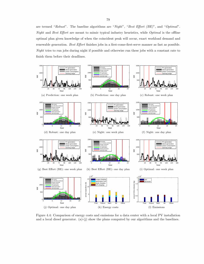
79

are termed “Robust”. The baseline algorithms are “Night”, “Best Effort (BE)”, and “Optimal”.

Night and Best Effort are meant to mimic typical industry heuristics, while Optimal is the offline

optimal plan given knowledge of when the coincident peak will occur, exact workload demand and

renewable generation. Best Effort finishes jobs in a first-come-first-serve manner as fast as possible.

Night tries to run jobs during night if possible and otherwise run these jobs with a constant rate to

finish them before their deadlines.

24 48 72 96 120 144 1680

500

1000

1500

hour

kW

PV generationdiesel generationpower consumptionwarning range

(a) Prediction: one week plan

0 6 12 18 240

500

1000

1500

hour

kW

idle powernon−flexible workloadflexible workloadcooling powerPV generationdiesel generationwarning range

(b) Prediction: one day plan

24 48 72 96 120 144 1680

500

1000

1500

hour

kW


(c) Robust: one week plan

0 6 12 18 240

500

1000

1500

hour

kW


(d) Robust: one day plan

24 48 72 96 120 144 1680

500

1000

1500

hour

kW


(e) Night: one week plan

0 6 12 18 240

500

1000

1500

hour

kW


(f) Night: one day plan

24 48 72 96 120 144 1680

500

1000

1500

hour

kW


(g) Best Effort (BE): one week plan

0 6 12 18 240

500

1000

1500

hour

kW


(h) Best Effort (BE): one day plan

24 48 72 96 120 144 1680

500

1000

1500

hour

kW


(i) Optimal: one week plan

0 6 12 18 240

500

1000

1500

hour

kW


(j) Optimal: one day plan

Pred. Robust Night BE Offline0

5

10

15

x 104

annu

al e

xpen

ditu

re (

$)

usage charginggeneration costpeak chargingCP charging

(k) Energy costs


0.5

1

1.5

2x 10

6

annu

al C

O2e

em

issi

on (

kg)

gridgenerator

(l) Emissions

Figure 4.4: Comparison of energy costs and emissions for a data center with a local PV installationand a local diesel generator. (a)-(j) show the plans computed by our algorithms and the baselines.

80

4.4.2 Experimental results

In our experimental results, we seek to explore the following issues: (i) How much cost and emission

savings can our algorithms achieve? How close to optimal are our algorithms on real workloads?

(ii) What are the relative benefits of local generation and workload shifting and a mixture of both

with respect to cost and emission reductions? (iii) What is the impact of errors in predictions of the

coincident peak and the corresponding warnings?

Cost savings and emissions reductions

We start with the key question for the chapter: how much cost and emission savings do our algorithms

provide? Figure 4.4 shows our main experimental results comparing our algorithms with baselines.

The weekly power profile for the first week of June 2011 is shown in the first plot for each algorithm,

including power consumption, PV generation and diesel generation, and coincident peak warnings.

The detailed daily power breakdown for the first Monday in June 2011 is shown in the second plot for

each algorithm, including idle power, power consumed by serving flexible workload and non-flexible

workload, cooling power, local generation and warnings. Further, the last two plots includes a cost

comparison and an emissions comparison for over one year of operation, including usage costs, peak

costs, CP costs, local generation costs, and emissions from both the grid power and local generation

used.

As shown in the figure, our algorithms provide 40% savings compared to Night and Best Effort.

Specifically, Prediction reshapes the flexible workload to prevent using the time slots that are likely

to be warning periods or the coincident peak as shown in Figures 4.4 (a) and (b), while Robust

tries to make the grid power usage as flat as possible as shown in Figures 4.4 (c) and (d). Both

algorithms try to fully utilize PV generation. In contrast, Night and Best Effort do not consider the

warnings, the coincident peak, or renewable generation. Therefore, they have significantly higher

coincident peak charges and local generation costs (Night has higher cost here because it wastes even

more renewable generation). Since the warning and coincident peak predictions are quite accurate,

Prediction works better than Robust and similar to Optimal.

Local generation versus workload shifting

A second important goal of this chapter is to understand the relative benefits of local generation

planning and workload shifting for data centers participating in CPP programs. Though our algo-

rithms have focused on the case of local generation, they can be easily adjusted to the case where

there is no local generator. In fact, similar analytic results hold for that case, but were omitted

due to space consideration. Instead, we use simulation results to explore this case. In particular,

to evaluate the relative benefits of local generation and workload shifting in practice, we can con-

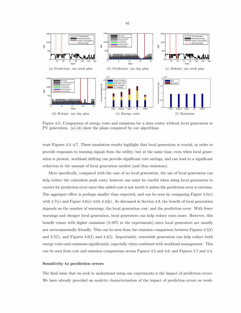
81

24 48 72 96 120 144 1680

500

1000

1500

hour

kW



0 6 12 18 240

500

1000

1500

hour

kW



24 48 72 96 120 144 1680

500

1000

1500

hour

kW



0 6 12 18 240

500

1000

1500

hour

kW




5

10

15

x 104

annu

al e

xpen

ditu

re (

$)


(e) Energy costs


0.5

1

1.5

2x 10

6

annu

al C

O2e

em

issi

on (

kg)

gridgenerator

(f) Emissions

Figure 4.5: Comparison of energy costs and emissions for a data center without local generation orPV generation. (a)-(d) show the plans computed by our algorithms.

trast Figures 4.4–4.7. These simulation results highlight that local generation is crucial, in order to

provide responses to warning signals from the utility; but at the same time, even when local gener-

ation is present, workload shifting can provide significant cost savings, and can lead to a significant

reduction in the amount of local generation needed (and thus emissions).

More specifically, compared with the case of no local generation, the use of local generation can

help reduce the coincident peak costs; however one must be careful when using local generation to

correct for prediction error since this added cost is not worth it unless the prediction error is extreme.

The aggregate effect is perhaps smaller than expected, and can be seen by comparing Figure 4.5(e)

with 4.7(e) and Figure 4.6(e) with 4.4(k). As discussed in Section 4.3, the benefit of local generation

depends on the number of warnings, the local generation cost, and the prediction error. With fewer

warnings and cheaper local generation, local generators can help reduce costs more. However, this

benefit comes with higher emissions (5-10% in the experiments) since local generators are usually

not environmentally friendly. This can be seen from the emission comparison between Figures 4.5(f)

and 4.7(f), and Figures 4.6(f) and 4.4(l). Importantly, renewable generation can help reduce both

energy costs and emissions significantly, especially when combined with workload management. This

can be seen from cost and emission comparisons across Figures 4.5 and 4.6, and Figures 4.7 and 4.4.

Sensitivity to prediction errors

The final issue that we seek to understand using our experiments is the impact of prediction errors.

We have already provided an analytic characterization of the impact of prediction errors on work-

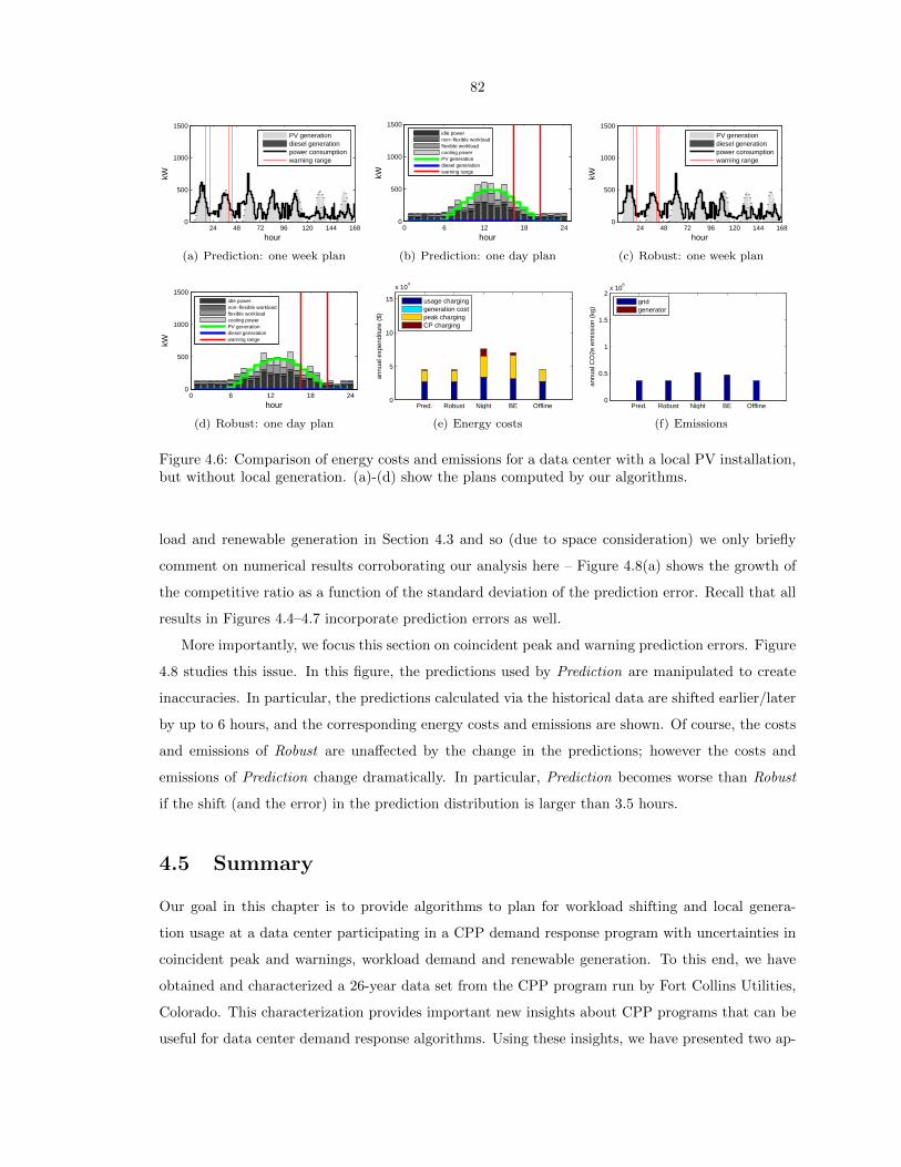
82

24 48 72 96 120 144 1680

500

1000

1500

hour

kW



0 6 12 18 240

500

1000

1500

hour

kW



24 48 72 96 120 144 1680

500

1000

1500

hour

kW



0 6 12 18 240

500

1000

1500

hour

kW




5

10

15

x 104

annu

al e

xpen

ditu

re (

$)


(e) Energy costs


0.5

1

1.5

2x 10

6

annu

al C

O2e

em

issi

on (

kg)

gridgenerator

(f) Emissions

Figure 4.6: Comparison of energy costs and emissions for a data center with a local PV installation,but without local generation. (a)-(d) show the plans computed by our algorithms.

load and renewable generation in Section 4.3 and so (due to space consideration) we only briefly

comment on numerical results corroborating our analysis here – Figure 4.8(a) shows the growth of

the competitive ratio as a function of the standard deviation of the prediction error. Recall that all

results in Figures 4.4–4.7 incorporate prediction errors as well.

More importantly, we focus this section on coincident peak and warning prediction errors. Figure

4.8 studies this issue. In this figure, the predictions used by Prediction are manipulated to create

inaccuracies. In particular, the predictions calculated via the historical data are shifted earlier/later

by up to 6 hours, and the corresponding energy costs and emissions are shown. Of course, the costs

and emissions of Robust are unaffected by the change in the predictions; however the costs and

emissions of Prediction change dramatically. In particular, Prediction becomes worse than Robust

if the shift (and the error) in the prediction distribution is larger than 3.5 hours.

4.5 Summary

Our goal in this chapter is to provide algorithms to plan for workload shifting and local genera-

tion usage at a data center participating in a CPP demand response program with uncertainties in

coincident peak and warnings, workload demand and renewable generation. To this end, we have

obtained and characterized a 26-year data set from the CPP program run by Fort Collins Utilities,

Colorado. This characterization provides important new insights about CPP programs that can be

useful for data center demand response algorithms. Using these insights, we have presented two ap-

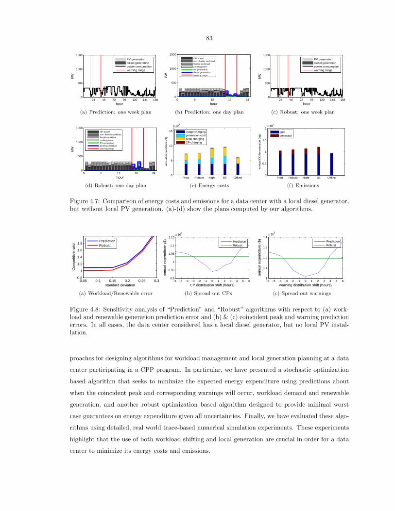
83

24 48 72 96 120 144 1680

500

1000

1500

hour

kW



0 6 12 18 240

500

1000

1500

hour

kW



24 48 72 96 120 144 1680

500

1000

1500

hour

kW



0 6 12 18 240

500

1000

1500

hour

kW




5

10

15

x 104

annu

al e

xpen

ditu

re (

$)


(e) Energy costs


0.5

1

1.5

2x 10

6

annu

al C

O2e

em

issi

on (

kg)

gridgenerator

(f) Emissions

Figure 4.7: Comparison of energy costs and emissions for a data center with a local diesel generator,but without local PV generation. (a)-(d) show the plans computed by our algorithms.

0.05 0.1 0.15 0.2 0.25 0.30.8

1

1.2

1.4

1.6

1.8

Com

petit

ive

ratio

standard deviation

PredictionRobust

(a) Workload/Renewable error

−6 −5 −4 −3 −2 −1 0 1 2 3 4 5 60.9

0.95

1

1.05

1.1

1.15x 10

5

CP distribution shift (hours)

annu

al e

xpen

ditu

re (

$)

PredictionRobust

(b) Spread out CPs

−6 −5 −4 −3 −2 −1 0 1 2 3 4 5 61

1.1

1.2

1.3

1.4x 10

5

warning distribution shift (hours)

annu

al e

xpen

ditu

re (

$)

PredictionRobust

(c) Spread out warnings

Figure 4.8: Sensitivity analysis of “Prediction” and “Robust” algorithms with respect to (a) work-load and renewable generation prediction error and (b) & (c) coincident peak and warning predictionerrors. In all cases, the data center considered has a local diesel generator, but no local PV instal-lation.

proaches for designing algorithms for workload management and local generation planning at a data

center participating in a CPP program. In particular, we have presented a stochastic optimization

based algorithm that seeks to minimize the expected energy expenditure using predictions about

when the coincident peak and corresponding warnings will occur, workload demand and renewable

generation, and another robust optimization based algorithm designed to provide minimal worst

case guarantees on energy expenditure given all uncertainties. Finally, we have evaluated these algo-

rithms using detailed, real world trace-based numerical simulation experiments. These experiments

highlight that the use of both workload shifting and local generation are crucial in order for a data

center to minimize its energy costs and emissions.

84

Chapter 5

IT for Sustainability: Pricing DataCenter Demand Response

Demand response is widely recognized as a crucial tool for incorporating renewables into the grid,

e.g., see recent reports from the National Institute of Standards and Technology (NIST) and the

Department of Energy (DoE) [140, 57]. Demand response programs provide incentives for customers

to adapt their electricity demand to supply availability, for example, reducing their consumption in

response to a peak load warning signal or request from the utility. Thus, demand response programs

can help the grid transition from the paradigm of “generation follows demand” to one where, at least

partially, “demand follows generation.” Such a transition is fundamental to the integration of re-

newable energy because generation is becoming more intermittent and less controllable as renewable

penetration increases.

In this chapter, we consider a promising demand response resource: data centers. Data centers

are particularly well-suited for demand response. First, data centers represent large loads for the grid.

In 2011, they consumed approximately 1.5% of all electricity worldwide and individual data centers

can be 50 MW, or more [79, 78, 160]. Further, the energy consumption of data centers is growing

quickly, by approximately 10-12% per year [78, 160, 110]. This growth is crucial for keeping pace

with the growth of renewable adoption predicted for the coming years. Third, and most importantly,

data centers are extremely flexible loads. Data centers are highly automated and monitored, e.g.,

the power load and state of IT equipment and cooling facilities can be continuously monitored

and panoramically adjusted. For example, a recent empirical study by LBNL has quantified the

flexibility in power usage of four data centers under different management approaches [78]. They

find that 5% of the load can typically be shed in 5 minutes and 10% of the load can be shed in

15 minutes; and that these can be achieved without changes to how the IT workload is handled,

i.e., via temperature adjustment and other building management approaches. Further, if workload

management approaches are considered, the degree of flexibility can be larger, without additional

time needed to shed the load. Significant research has recently gone into the design of such workload

85

management, e.g., [70, 44, 120, 86, 132, 197, 188, 193].

Data center demand response today

Despite wide recognition of the demand response potential of data centers, the current reality is that

data centers perform little, if any, demand response [79, 78].

In particular, the most common demand response program available for data centers is Coincident

Peak Pricing (CPP), which is required for medium and large industrial consumers in many regions.

These programs work by charging a very high price for usage during the coincident peak hour,

often over 200 times higher than the base rate.1 It is common for the coincident peak charges to

account for 23% or more of a customer’s electric bill according to Fort Collins Utilities [67]. Hence,

a customer has a strong incentive to reduce usage during the peak hour. Although it is impossible

to accurately predict exactly when the peak hour will occur, many utilities identify potential peak

hours and send warning signals to customers (5-10 per month), which helps customers manage their

loads and make decisions about their energy usage. For more details about CPP see [67].

Unfortunately, CPP programs are poorly designed from the perspective of data center demand

response. Not providing response may incur a very large charge and providing a response may not

actually result in any savings if the coincident peak does not occur during the warning period. As a

result, even when they are forced to participate in such programs, data centers tend not to actively

respond to signals. Further, even if they do respond, such programs extract very little flexibility

from data centers. At best they obtain curtailment of usage a few times per month. This wastes

the potential responsiveness of data centers.

Demand response market design

Although researchers have begun to focus on new market designs for data center demand response,

e.g., [174, 103, 78, 67, 171], a clear vision remains elusive.

This is also true outside of the domain of data centers. Recently, the design of demand response

programs has received considerable attention in a variety of settings, e.g., electric vehicles, pool

pumps, and air conditioner cycling. Broadly speaking, the demand response programs that have

emerged can be classified into two categories based on the interaction with users: either (i) users bid

some degree of flexibility (supply) into the market, usually via a parameterized supply function, or (ii)

users respond to a posted price, which was chosen using predictions about the available flexibility

(e.g., supply functions). We term these approaches “supply function bidding” and “prediction-

based pricing”, respectively. Examples of proposed designs that use supply function bidding include

[105, 191], and examples of prediction-based pricing designs include [48, 136, 118].

1The coincident peak hour is defined as the hour when the most electricity is demanded from the load servingentity (LSE).

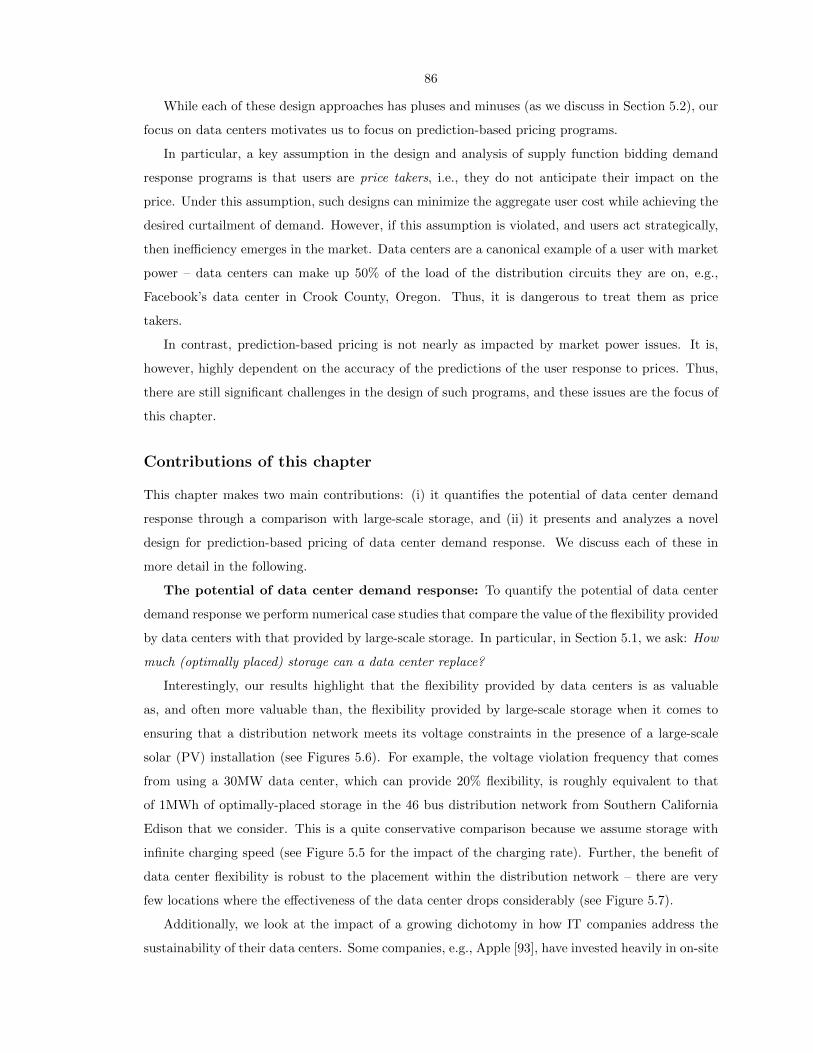
86

While each of these design approaches has pluses and minuses (as we discuss in Section 5.2), our

focus on data centers motivates us to focus on prediction-based pricing programs.

In particular, a key assumption in the design and analysis of supply function bidding demand

response programs is that users are price takers, i.e., they do not anticipate their impact on the

price. Under this assumption, such designs can minimize the aggregate user cost while achieving the

desired curtailment of demand. However, if this assumption is violated, and users act strategically,

then inefficiency emerges in the market. Data centers are a canonical example of a user with market

power – data centers can make up 50% of the load of the distribution circuits they are on, e.g.,

Facebook’s data center in Crook County, Oregon. Thus, it is dangerous to treat them as price

takers.

In contrast, prediction-based pricing is not nearly as impacted by market power issues. It is,

however, highly dependent on the accuracy of the predictions of the user response to prices. Thus,

there are still significant challenges in the design of such programs, and these issues are the focus of

this chapter.

Contributions of this chapter

This chapter makes two main contributions: (i) it quantifies the potential of data center demand

response through a comparison with large-scale storage, and (ii) it presents and analyzes a novel

design for prediction-based pricing of data center demand response. We discuss each of these in

more detail in the following.

The potential of data center demand response: To quantify the potential of data center

demand response we perform numerical case studies that compare the value of the flexibility provided

by data centers with that provided by large-scale storage. In particular, in Section 5.1, we ask: How

much (optimally placed) storage can a data center replace?

Interestingly, our results highlight that the flexibility provided by data centers is as valuable

as, and often more valuable than, the flexibility provided by large-scale storage when it comes to

ensuring that a distribution network meets its voltage constraints in the presence of a large-scale

solar (PV) installation (see Figures 5.6). For example, the voltage violation frequency that comes

from using a 30MW data center, which can provide 20% flexibility, is roughly equivalent to that

of 1MWh of optimally-placed storage in the 46 bus distribution network from Southern California

Edison that we consider. This is a quite conservative comparison because we assume storage with

infinite charging speed (see Figure 5.5 for the impact of the charging rate). Further, the benefit of

data center flexibility is robust to the placement within the distribution network – there are very

few locations where the effectiveness of the data center drops considerably (see Figure 5.7).

Additionally, we look at the impact of a growing dichotomy in how IT companies address the

sustainability of their data centers. Some companies, e.g., Apple [93], have invested heavily in on-site

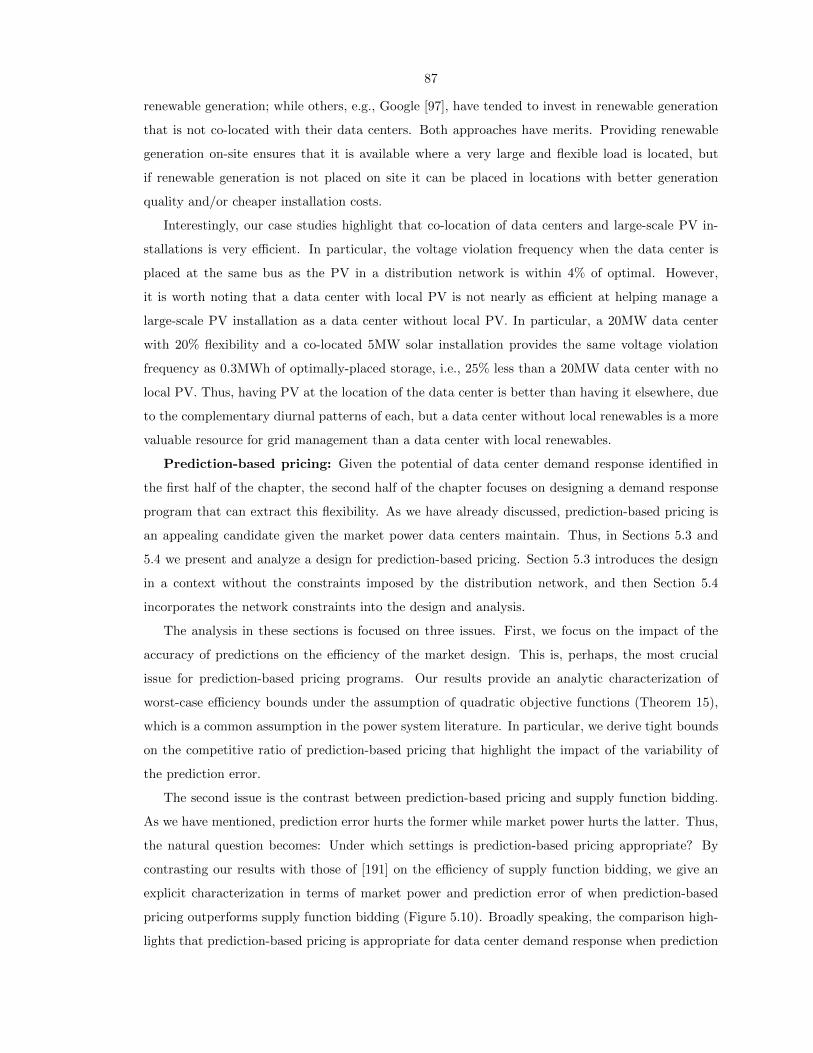
87

renewable generation; while others, e.g., Google [97], have tended to invest in renewable generation

that is not co-located with their data centers. Both approaches have merits. Providing renewable

generation on-site ensures that it is available where a very large and flexible load is located, but

if renewable generation is not placed on site it can be placed in locations with better generation

quality and/or cheaper installation costs.

Interestingly, our case studies highlight that co-location of data centers and large-scale PV in-

stallations is very efficient. In particular, the voltage violation frequency when the data center is

placed at the same bus as the PV in a distribution network is within 4% of optimal. However,

it is worth noting that a data center with local PV is not nearly as efficient at helping manage a

large-scale PV installation as a data center without local PV. In particular, a 20MW data center

with 20% flexibility and a co-located 5MW solar installation provides the same voltage violation

frequency as 0.3MWh of optimally-placed storage, i.e., 25% less than a 20MW data center with no

local PV. Thus, having PV at the location of the data center is better than having it elsewhere, due

to the complementary diurnal patterns of each, but a data center without local renewables is a more

valuable resource for grid management than a data center with local renewables.

Prediction-based pricing: Given the potential of data center demand response identified in

the first half of the chapter, the second half of the chapter focuses on designing a demand response

program that can extract this flexibility. As we have already discussed, prediction-based pricing is

an appealing candidate given the market power data centers maintain. Thus, in Sections 5.3 and

5.4 we present and analyze a design for prediction-based pricing. Section 5.3 introduces the design

in a context without the constraints imposed by the distribution network, and then Section 5.4

incorporates the network constraints into the design and analysis.

The analysis in these sections is focused on three issues. First, we focus on the impact of the

accuracy of predictions on the efficiency of the market design. This is, perhaps, the most crucial

issue for prediction-based pricing programs. Our results provide an analytic characterization of

worst-case efficiency bounds under the assumption of quadratic objective functions (Theorem 15),

which is a common assumption in the power system literature. In particular, we derive tight bounds

on the competitive ratio of prediction-based pricing that highlight the impact of the variability of

the prediction error.

The second issue is the contrast between prediction-based pricing and supply function bidding.

As we have mentioned, prediction error hurts the former while market power hurts the latter. Thus,

the natural question becomes: Under which settings is prediction-based pricing appropriate? By

contrasting our results with those of [191] on the efficiency of supply function bidding, we give an

explicit characterization in terms of market power and prediction error of when prediction-based

pricing outperforms supply function bidding (Figure 5.10). Broadly speaking, the comparison high-

lights that prediction-based pricing is appropriate for data center demand response when prediction

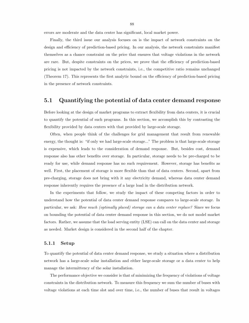
88

errors are moderate and the data center has significant, local market power.

Finally, the third issue our analysis focuses on is the impact of network constraints on the

design and efficiency of prediction-based pricing. In our analysis, the network constraints manifest

themselves as a chance constraint on the price that ensures that voltage violations in the network

are rare. But, despite constraints on the prices, we prove that the efficiency of prediction-based

pricing is not impacted by the network constraints, i.e., the competitive ratio remains unchanged

(Theorem 17). This represents the first analytic bound on the efficiency of prediction-based pricing

in the presence of network constraints.

5.1 Quantifying the potential of data center demand response

Before looking at the design of market programs to extract flexibility from data centers, it is crucial

to quantify the potential of such programs. In this section, we accomplish this by contrasting the

flexibility provided by data centers with that provided by large-scale storage.

Often, when people think of the challenges for grid management that result from renewable

energy, the thought is: “if only we had large-scale storage...” The problem is that large-scale storage

is expensive, which leads to the consideration of demand response. But, besides cost, demand

response also has other benefits over storage. In particular, storage needs to be pre-charged to be

ready for use, while demand response has no such requirement. However, storage has benefits as

well. First, the placement of storage is more flexible than that of data centers. Second, apart from

pre-charging, storage does not bring with it any electricity demand, whereas data center demand

response inherently requires the presence of a large load in the distribution network.

In the experiments that follow, we study the impact of these competing factors in order to

understand how the potential of data center demand response compares to large-scale storage. In

particular, we ask: How much (optimally placed) storage can a data center replace? Since we focus

on bounding the potential of data center demand response in this section, we do not model market

factors. Rather, we assume that the load serving entity (LSE) can call on the data center and storage

as needed. Market design is considered in the second half of the chapter.

5.1.1 Setup

To quantify the potential of data center demand response, we study a situation where a distribution

network has a large-scale solar installation and either large-scale storage or a data center to help

manage the intermittency of the solar installation.

The performance objective we consider is that of minimizing the frequency of violations of voltage

constraints in the distribution network. To measure this frequency we sum the number of buses with

voltage violations at each time slot and over time, i.e., the number of buses that result in voltages

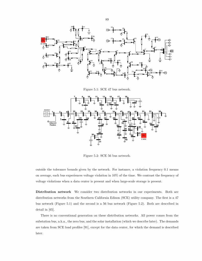
89

Figure 5.1: SCE 47 bus network.

Figure 5.2: SCE 56 bus network.

outside the tolerance bounds given by the network. For instance, a violation frequency 0.1 means

on average, each bus experiences voltage violation in 10% of the time. We contrast the frequency of

voltage violations when a data center is present and when large-scale storage is present.

Distribution network We consider two distribution networks in our experiments. Both are

distribution networks from the Southern California Edison (SCE) utility company. The first is a 47

bus network (Figure 5.1) and the second is a 56 bus network (Figure 5.2). Both are described in

detail in [65].

There is no conventional generation on these distribution networks. All power comes from the

substation bus, a.k.a., the zero bus, and the solar installation (which we describe later). The demands

are taken from SCE load profiles [91], except for the data center, for which the demand is described

later.

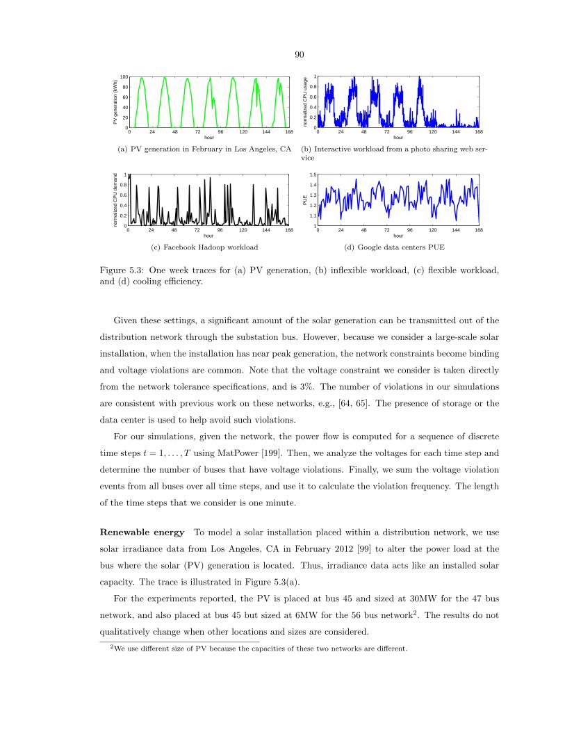
90

0 24 48 72 96 120 144 1680

20

40

60

80

100

hour

PV

gen

erat

ion

(kW

h)

(a) PV generation in February in Los Angeles, CA

0 24 48 72 96 120 144 1680

0.2

0.4

0.6

0.8

1

hour

norm

aliz

ed C

PU

usa

ge

(b) Interactive workload from a photo sharing web ser-vice

0 24 48 72 96 120 144 1680

0.2

0.4

0.6

0.8

1

hour

norm

aliz

ed C

PU

dem

and

(c) Facebook Hadoop workload

0 24 48 72 96 120 144 1681

1.1

1.2

1.3

1.4

1.5

hour

PU

E

(d) Google data centers PUE

Figure 5.3: One week traces for (a) PV generation, (b) inflexible workload, (c) flexible workload,and (d) cooling efficiency.

Given these settings, a significant amount of the solar generation can be transmitted out of the

distribution network through the substation bus. However, because we consider a large-scale solar

installation, when the installation has near peak generation, the network constraints become binding

and voltage violations are common. Note that the voltage constraint we consider is taken directly

from the network tolerance specifications, and is 3%. The number of violations in our simulations

are consistent with previous work on these networks, e.g., [64, 65]. The presence of storage or the

data center is used to help avoid such violations.

For our simulations, given the network, the power flow is computed for a sequence of discrete

time steps t = 1, . . . , T using MatPower [199]. Then, we analyze the voltages for each time step and

determine the number of buses that have voltage violations. Finally, we sum the voltage violation

events from all buses over all time steps, and use it to calculate the violation frequency. The length

of the time steps that we consider is one minute.

Renewable energy To model a solar installation placed within a distribution network, we use

solar irradiance data from Los Angeles, CA in February 2012 [99] to alter the power load at the

bus where the solar (PV) generation is located. Thus, irradiance data acts like an installed solar

capacity. The trace is illustrated in Figure 5.3(a).

For the experiments reported, the PV is placed at bus 45 and sized at 30MW for the 47 bus

network, and also placed at bus 45 but sized at 6MW for the 56 bus network2. The results do not

qualitatively change when other locations and sizes are considered.

2We use different size of PV because the capacities of these two networks are different.

91

Data center model To incorporate a data center into the experiments, we need to model two

aspects: the power usage of the data center over time and the flexibility in the power usage of the

data center.

To model the power usage of a data center, we adopt the model used in [120, 119, 130, 14], which

provides a simple but representative characterization. In particular, we model the power demand of

the data center as a function of the workload, including interactive (inflexible) and delay-tolerant

(flexible) workloads, and the cooling efficiency, as measured by the Power Usage Effectiveness (PUE).

To model the workload we use two traces. The interactive workload trace is from a popular web

service application with more than 85 million registered users in 22 countries (see Figure 5.3(b)).

The trace contains average CPU utilization and memory usage as recorded every 5 minutes. The

peak-to-mean ratio of the interactive workload is about 4. The delay-tolerant workload information

comes from a Facebook Hadoop trace (see Figure 5.3(c)). The total demand ratio between the

interactive workload and batch jobs is 1:1. This ratio can vary widely across data centers, but we

choose this ratio as representative based on discussions in [121].

To model the data center power efficiency including cooling efficiency, we use a trace of the PUE

from Google data centers. As shown in the figure, the PUE varies between 1.05 to 1.45, and has

strong diurnal pattern, i.e., higher around noon because outside air temperature is higher.

To combine the workload traces and the PUE to obtain a model of the total power demand of

the data center, we use the following relationship.

v(t) = PUE(t)(a(t) + b(t)),

where a(t) is the power demand from the inflexible workload and b(t) is power demand from the

flexible workload demand. Note that the data center power demand has the same average value as

the PV generation with the same capacity in the distribution network.

The second aspect of the data center model that we must include is the flexibility of the power

demand. For this, our model is informed by the recent empirical study [78], which we have discussed

in the introduction.

To model the range of flexibility in our experiments, we denote the demand flexibility of the data

center by e and allow the data center to have demand within

[(1− e)v(t),min(1 + e)v(t), Cd],

where Cd is the capacity of the data center and v(t) is the data center power demand at time t if no

demand response is called upon. Thus, e = 0.10 could be achieved without workload management,

and e = 0.20 can be achieved with some workload management, e.g., quality degradation or load

deferral. When demand response is required from the data center, the load that minimizes the

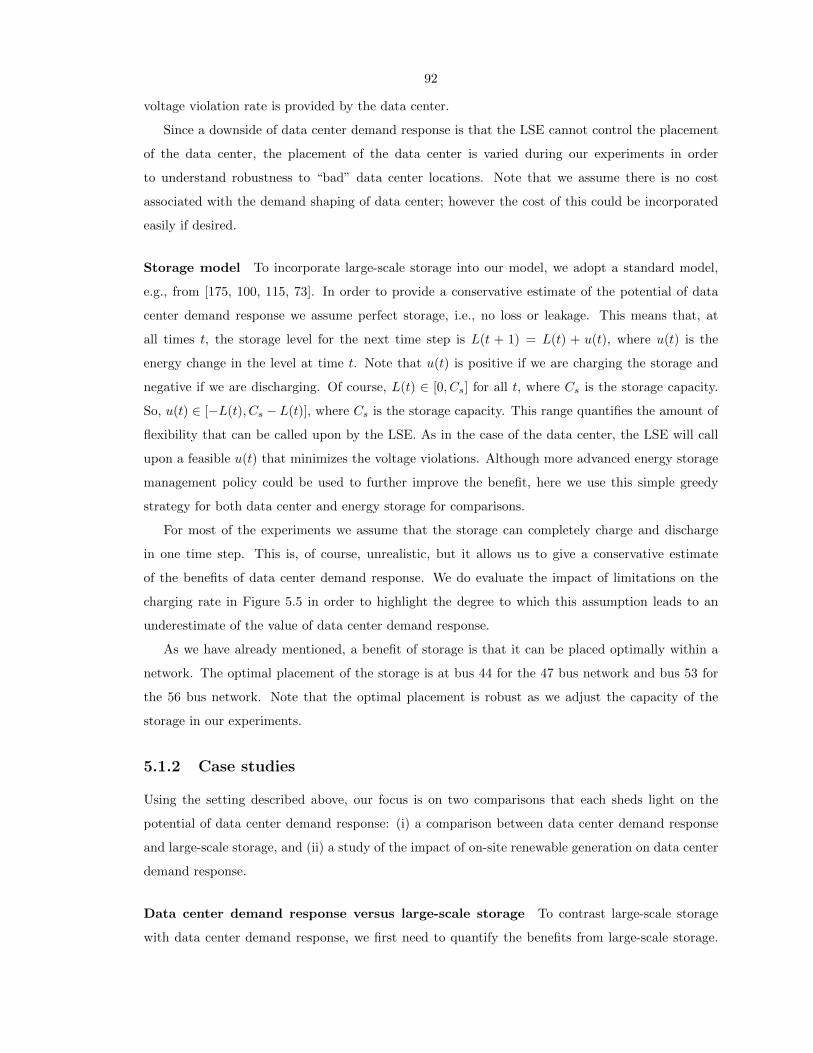
92

voltage violation rate is provided by the data center.

Since a downside of data center demand response is that the LSE cannot control the placement

of the data center, the placement of the data center is varied during our experiments in order

to understand robustness to “bad” data center locations. Note that we assume there is no cost

associated with the demand shaping of data center; however the cost of this could be incorporated

easily if desired.

Storage model To incorporate large-scale storage into our model, we adopt a standard model,

e.g., from [175, 100, 115, 73]. In order to provide a conservative estimate of the potential of data

center demand response we assume perfect storage, i.e., no loss or leakage. This means that, at

all times t, the storage level for the next time step is L(t + 1) = L(t) + u(t), where u(t) is the

energy change in the level at time t. Note that u(t) is positive if we are charging the storage and

negative if we are discharging. Of course, L(t) ∈ [0, Cs] for all t, where Cs is the storage capacity.

So, u(t) ∈ [−L(t), Cs − L(t)], where Cs is the storage capacity. This range quantifies the amount of

flexibility that can be called upon by the LSE. As in the case of the data center, the LSE will call

upon a feasible u(t) that minimizes the voltage violations. Although more advanced energy storage

management policy could be used to further improve the benefit, here we use this simple greedy

strategy for both data center and energy storage for comparisons.

For most of the experiments we assume that the storage can completely charge and discharge

in one time step. This is, of course, unrealistic, but it allows us to give a conservative estimate

of the benefits of data center demand response. We do evaluate the impact of limitations on the

charging rate in Figure 5.5 in order to highlight the degree to which this assumption leads to an

underestimate of the value of data center demand response.

As we have already mentioned, a benefit of storage is that it can be placed optimally within a

network. The optimal placement of the storage is at bus 44 for the 47 bus network and bus 53 for

the 56 bus network. Note that the optimal placement is robust as we adjust the capacity of the

storage in our experiments.

5.1.2 Case studies

Using the setting described above, our focus is on two comparisons that each sheds light on the

potential of data center demand response: (i) a comparison between data center demand response

and large-scale storage, and (ii) a study of the impact of on-site renewable generation on data center

demand response.

Data center demand response versus large-scale storage To contrast large-scale storage

with data center demand response, we first need to quantify the benefits from large-scale storage.

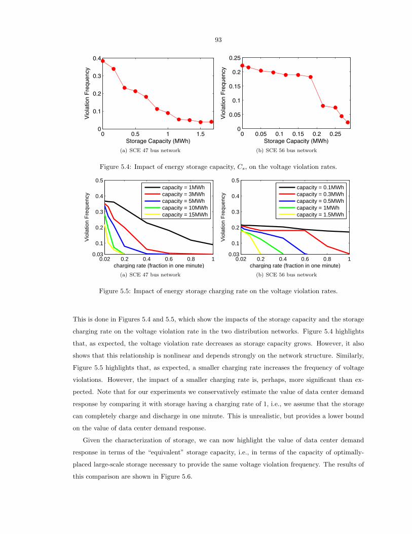
93

0 0.5 1 1.50

0.1

0.2

0.3

0.4

Storage Capacity (MWh)

Viol

atio

n Fr

eque

ncy

(a) SCE 47 bus network

0 0.05 0.1 0.15 0.2 0.250

0.05

0.1

0.15

0.2

0.25

Storage Capacity (MWh)

Viol

atio

n Fr

eque

ncy

(b) SCE 56 bus network

Figure 5.4: Impact of energy storage capacity, Cs, on the voltage violation rates.

0.02 0.2 0.4 0.6 0.8 10.03

0.1

0.2

0.3

0.4

0.5

charging rate (fraction in one minute)

Vio

latio

n F

requ

ency

capacity = 1MWhcapacity = 3MWhcapacity = 5MWhcapacity = 10MWhcapacity = 15MWh


0.02 0.2 0.4 0.6 0.8 10.03

0.1

0.2

0.3

0.4

0.5

charging rate (fraction in one minute)

Vio

latio

n F

requ

ency

capacity = 0.1MWhcapacity = 0.3MWhcapacity = 0.5MWhcapacity = 1MWhcapacity = 1.5MWh


Figure 5.5: Impact of energy storage charging rate on the voltage violation rates.

This is done in Figures 5.4 and 5.5, which show the impacts of the storage capacity and the storage

charging rate on the voltage violation rate in the two distribution networks. Figure 5.4 highlights

that, as expected, the voltage violation rate decreases as storage capacity grows. However, it also

shows that this relationship is nonlinear and depends strongly on the network structure. Similarly,

Figure 5.5 highlights that, as expected, a smaller charging rate increases the frequency of voltage

violations. However, the impact of a smaller charging rate is, perhaps, more significant than ex-

pected. Note that for our experiments we conservatively estimate the value of data center demand

response by comparing it with storage having a charging rate of 1, i.e., we assume that the storage

can completely charge and discharge in one minute. This is unrealistic, but provides a lower bound

on the value of data center demand response.

Given the characterization of storage, we can now highlight the value of data center demand

response in terms of the “equivalent” storage capacity, i.e., in terms of the capacity of optimally-

placed large-scale storage necessary to provide the same voltage violation frequency. The results of

this comparison are shown in Figure 5.6.

94

Naturally, the amount of storage equivalent to data center demand response grows with the

size of the data center. However, the capacity plateaus after the data center size grows beyond

35MW for the SCE 47 bus network and beyond 6MW for the SCE 56 bus network. Note that this

is a consequence of two differences between the networks – the structure and the size of the PV

installation (30MW vs. 6MW).

But, in both networks, Figure 5.6 highlights that data center demand response has a signifi-

cant potential. In particular, recall that the comparison in this plot assumes storage with infinite

charging speed, i.e., a charging rate of 1, and is thus quite conservative (as illustrated in Figure

5.5). Additionally, the cost of storage is upwards of $500/kWh for lithium-ion batteries (which have

small charging rates) and upwards of $5000/kWh for technologies with fast charging rates, such as

flywheels. Thus, the flexibility provided by one 30MW data center is worth upwards of $500,000 -

$5,000,000. These numbers are conservative estimates, and grow considerably if a slower charging

rate is used in the simulations or if the flexibility of the data center, e, is increased.

Figures 5.7 and 5.8 delve into the comparison of data center demand response and large-scale

storage in more detail for each of the networks. In Figure 5.7, we fix the capacity of the data

center to 20MW, which is a representative size for today’s IT companies, and then investigate the

impact of the degree of data center flexibility, e, and the placement of the data center. For example,

Figures 5.7(a)-5.7(c) highlight that the voltage violation rates decrease as data center power demand

becomes more flexible. In particular, a 20MW data center with 20% power demand flexibility placed

at the PV location is equivalent to 0.67MWh of optimally-placed storage in the 47 bus distribution

network. Further, Figure 5.7(d) shows that the benefit of data center flexibility is robust to the

placement of the network in the distribution network, i.e., there are very few locations where the

effectiveness of the data center drops considerably and many locations that are near-optimal, e.g.,

placing the data center at the location of the PV (Figure 5.7(b)). Figure 5.7(d) also illustrates that

a 20MW data center is better than 0.33MWh of storage pretty much uniformly. The results in a

SCE 56 bus network are similar, as shown in Figure 5.8.

Should data centers invest in co-located renewables? There is a dichotomy right now in

how IT companies address the sustainability of their data centers. Some companies, e.g., Apple [93],

have invested heavily in on-site renewable generation; while others, e.g., Google [97], have tended to

invest in renewable generation that is not co-located with their data centers.

Both approaches have merits, as we have discussed in the introduction. For the purpose of

this chapter, the key distinction is how on-site renewable generation impacts data center demand

response. This context highlights another benefit of on site renewable generation – it ensures that

the data center is placed close to the renewables, which is very often a near-optimal placement for

demand response purposes.

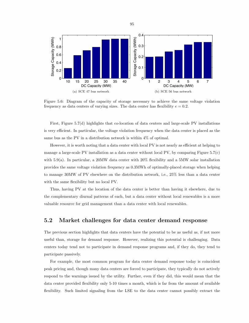
95

10 15 20 25 30 35 400

0.2

0.4

0.6

0.8

1

DC Capacity (MW)

Stor

age

Cap

acity

(MW

h)


1 2 3 4 5 6 70

0.1

0.2

0.3

0.4

DC Capacity (MW)

Stor

age

Cap

acity

(MW

h)


Figure 5.6: Diagram of the capacity of storage necessary to achieve the same voltage violationfrequency as data centers of varying sizes. The data center has flexibility e = 0.2.

First, Figure 5.7(d) highlights that co-location of data centers and large-scale PV installations

is very efficient. In particular, the voltage violation frequency when the data center is placed as the

same bus as the PV in a distribution network is within 4% of optimal.

However, it is worth noting that a data center with local PV is not nearly as efficient at helping to

manage a large-scale PV installation as a data center without local PV, by comparing Figure 5.7(c)

with 5.9(a). In particular, a 20MW data center with 20% flexibility and a 5MW solar installation

provides the same voltage violation frequency as 0.3MWh of optimally-placed storage when helping

to manage 30MW of PV elsewhere on the distribution network, i.e., 25% less than a data center

with the same flexibility but no local PV.

Thus, having PV at the location of the data center is better than having it elsewhere, due to

the complementary diurnal patterns of each, but a data center without local renewables is a more

valuable resource for grid management than a data center with local renewables.

5.2 Market challenges for data center demand response

The previous section highlights that data centers have the potential to be as useful as, if not more

useful than, storage for demand response. However, realizing this potential is challenging. Data

centers today tend not to participate in demand response programs and, if they do, they tend to

participate passively.

For example, the most common program for data center demand response today is coincident

peak pricing and, though many data centers are forced to participate, they typically do not actively

respond to the warnings issued by the utility. Further, even if they did, this would mean that the

data center provided flexibility only 5-10 times a month, which is far from the amount of available

flexibility. Such limited signaling from the LSE to the data center cannot possibly extract the

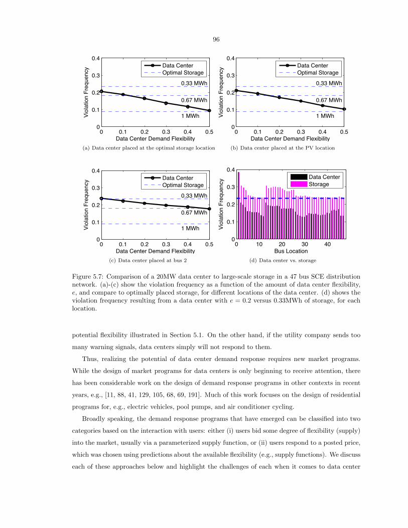
96

0 0.1 0.2 0.3 0.4 0.50

0.1

0.2

0.3

0.4

0.33 MWh

0.67 MWh

1 MWh

Data Center Demand Flexibility

Viol

atio

n Fr

eque

ncy

Data CenterOptimal Storage

(a) Data center placed at the optimal storage location

0 0.1 0.2 0.3 0.4 0.50

0.1

0.2

0.3

0.4

0.33 MWh

0.67 MWh

1 MWh


Viol

atio

n Fr

eque

ncy


(b) Data center placed at the PV location

0 0.1 0.2 0.3 0.4 0.50

0.1

0.2

0.3

0.4

0.33 MWh

0.67 MWh

1 MWh


Viol

atio

n Fr

eque

ncy


(c) Data center placed at bus 2

0 10 20 30 400

0.1

0.2

0.3

0.4

Bus Location

Viol

atio

n Fr

eque

ncy

Data CenterStorage

(d) Data center vs. storage

Figure 5.7: Comparison of a 20MW data center to large-scale storage in a 47 bus SCE distributionnetwork. (a)-(c) show the violation frequency as a function of the amount of data center flexibility,e, and compare to optimally placed storage, for different locations of the data center. (d) shows theviolation frequency resulting from a data center with e = 0.2 versus 0.33MWh of storage, for eachlocation.

potential flexibility illustrated in Section 5.1. On the other hand, if the utility company sends too

many warning signals, data centers simply will not respond to them.

Thus, realizing the potential of data center demand response requires new market programs.

While the design of market programs for data centers is only beginning to receive attention, there

has been considerable work on the design of demand response programs in other contexts in recent

years, e.g., [11, 88, 41, 129, 105, 68, 69, 191]. Much of this work focuses on the design of residential

programs for, e.g., electric vehicles, pool pumps, and air conditioner cycling.

Broadly speaking, the demand response programs that have emerged can be classified into two

categories based on the interaction with users: either (i) users bid some degree of flexibility (supply)

into the market, usually via a parameterized supply function, or (ii) users respond to a posted price,

which was chosen using predictions about the available flexibility (e.g., supply functions). We discuss

each of these approaches below and highlight the challenges of each when it comes to data center

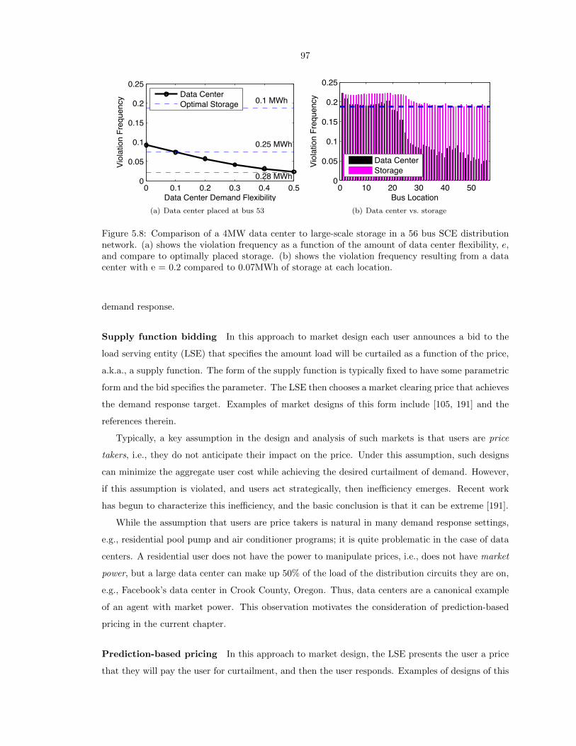
97

0 0.1 0.2 0.3 0.4 0.50

0.05

0.1

0.15

0.2

0.25

0.1 MWh

0.25 MWh

0.28 MWh


Viol

atio

n Fr

eque

ncy


(a) Data center placed at bus 53

0 10 20 30 40 500

0.05

0.1

0.15

0.2

0.25

Bus Location

Viol

atio

n Fr

eque

ncy

Data CenterStorage

(b) Data center vs. storage

Figure 5.8: Comparison of a 4MW data center to large-scale storage in a 56 bus SCE distributionnetwork. (a) shows the violation frequency as a function of the amount of data center flexibility, e,and compare to optimally placed storage. (b) shows the violation frequency resulting from a datacenter with e = 0.2 compared to 0.07MWh of storage at each location.

demand response.

Supply function bidding In this approach to market design each user announces a bid to the

load serving entity (LSE) that specifies the amount load will be curtailed as a function of the price,

a.k.a., a supply function. The form of the supply function is typically fixed to have some parametric

form and the bid specifies the parameter. The LSE then chooses a market clearing price that achieves

the demand response target. Examples of market designs of this form include [105, 191] and the

references therein.

Typically, a key assumption in the design and analysis of such markets is that users are price

takers, i.e., they do not anticipate their impact on the price. Under this assumption, such designs

can minimize the aggregate user cost while achieving the desired curtailment of demand. However,

if this assumption is violated, and users act strategically, then inefficiency emerges. Recent work

has begun to characterize this inefficiency, and the basic conclusion is that it can be extreme [191].

While the assumption that users are price takers is natural in many demand response settings,

e.g., residential pool pump and air conditioner programs; it is quite problematic in the case of data

centers. A residential user does not have the power to manipulate prices, i.e., does not have market

power, but a large data center can make up 50% of the load of the distribution circuits they are on,

e.g., Facebook’s data center in Crook County, Oregon. Thus, data centers are a canonical example

of an agent with market power. This observation motivates the consideration of prediction-based

pricing in the current chapter.

Prediction-based pricing In this approach to market design, the LSE presents the user a price

that they will pay the user for curtailment, and then the user responds. Examples of designs of this

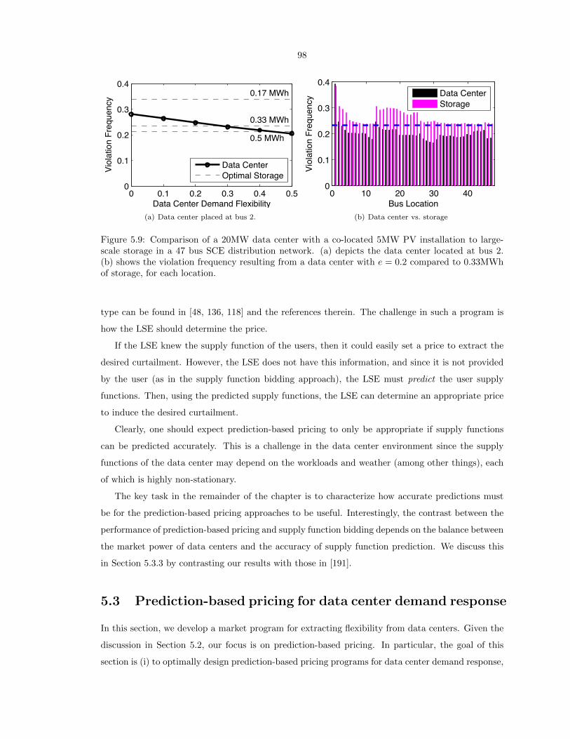
98

0 0.1 0.2 0.3 0.4 0.50

0.1

0.2

0.3

0.40.17 MWh

0.33 MWh

0.5 MWh


Viol

atio

n Fr

eque

ncy


(a) Data center placed at bus 2.

0 10 20 30 400

0.1

0.2

0.3

0.4

Bus Location

Viol

atio

n Fr

eque

ncy

Data CenterStorage

(b) Data center vs. storage

Figure 5.9: Comparison of a 20MW data center with a co-located 5MW PV installation to large-scale storage in a 47 bus SCE distribution network. (a) depicts the data center located at bus 2.(b) shows the violation frequency resulting from a data center with e = 0.2 compared to 0.33MWhof storage, for each location.

type can be found in [48, 136, 118] and the references therein. The challenge in such a program is

how the LSE should determine the price.

If the LSE knew the supply function of the users, then it could easily set a price to extract the

desired curtailment. However, the LSE does not have this information, and since it is not provided

by the user (as in the supply function bidding approach), the LSE must predict the user supply

functions. Then, using the predicted supply functions, the LSE can determine an appropriate price

to induce the desired curtailment.

Clearly, one should expect prediction-based pricing to only be appropriate if supply functions

can be predicted accurately. This is a challenge in the data center environment since the supply

functions of the data center may depend on the workloads and weather (among other things), each

of which is highly non-stationary.

The key task in the remainder of the chapter is to characterize how accurate predictions must

be for the prediction-based pricing approaches to be useful. Interestingly, the contrast between the

performance of prediction-based pricing and supply function bidding depends on the balance between

the market power of data centers and the accuracy of supply function prediction. We discuss this

in Section 5.3.3 by contrasting our results with those in [191].

5.3 Prediction-based pricing for data center demand response

In this section, we develop a market program for extracting flexibility from data centers. Given the

discussion in Section 5.2, our focus is on prediction-based pricing. In particular, the goal of this

section is (i) to optimally design prediction-based pricing programs for data center demand response,

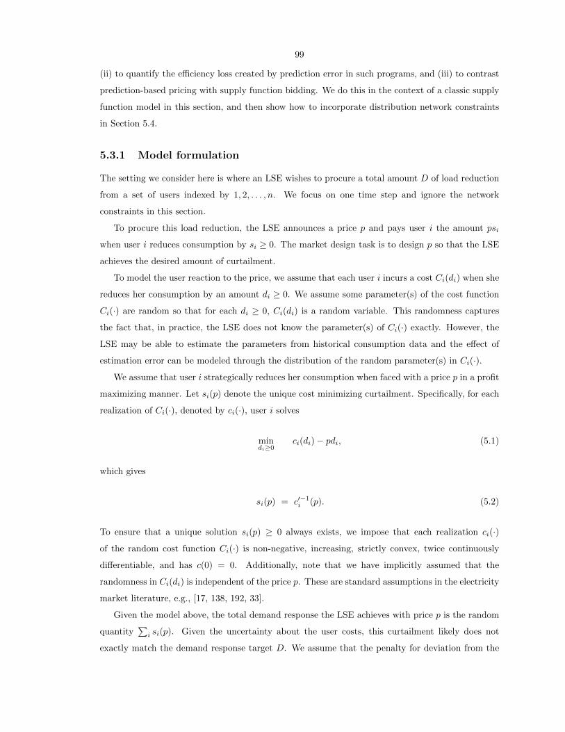
99

(ii) to quantify the efficiency loss created by prediction error in such programs, and (iii) to contrast

prediction-based pricing with supply function bidding. We do this in the context of a classic supply

function model in this section, and then show how to incorporate distribution network constraints

in Section 5.4.

5.3.1 Model formulation

The setting we consider here is where an LSE wishes to procure a total amount D of load reduction

from a set of users indexed by 1, 2, . . . , n. We focus on one time step and ignore the network

constraints in this section.

To procure this load reduction, the LSE announces a price p and pays user i the amount psi

when user i reduces consumption by si ≥ 0. The market design task is to design p so that the LSE

achieves the desired amount of curtailment.

To model the user reaction to the price, we assume that each user i incurs a cost Ci(di) when she

reduces her consumption by an amount di ≥ 0. We assume some parameter(s) of the cost function

Ci(·) are random so that for each di ≥ 0, Ci(di) is a random variable. This randomness captures

the fact that, in practice, the LSE does not know the parameter(s) of Ci(·) exactly. However, the

LSE may be able to estimate the parameters from historical consumption data and the effect of

estimation error can be modeled through the distribution of the random parameter(s) in Ci(·).

We assume that user i strategically reduces her consumption when faced with a price p in a profit

maximizing manner. Let si(p) denote the unique cost minimizing curtailment. Specifically, for each

realization of Ci(·), denoted by ci(·), user i solves

mindi≥0

ci(di)− pdi, (5.1)

which gives

si(p) = c′−1i (p). (5.2)

To ensure that a unique solution si(p) ≥ 0 always exists, we impose that each realization ci(·)

of the random cost function Ci(·) is non-negative, increasing, strictly convex, twice continuously

differentiable, and has c(0) = 0. Additionally, note that we have implicitly assumed that the

randomness in Ci(di) is independent of the price p. These are standard assumptions in the electricity

market literature, e.g., [17, 138, 192, 33].

Given the model above, the total demand response the LSE achieves with price p is the random

quantity∑i si(p). Given the uncertainty about the user costs, this curtailment likely does not

exactly match the demand response target D. We assume that the penalty for deviation from the

100

target is captured through a penalty function h(·). In particular, the penalty is h (D −∑i si(p)).

We assume this penalty function h(·) is convex, non-negative, has a global minimum h(0) = 0, and

is continuously differentiable with h′(0) = 0. These assumptions ensure that the optimal price is

well-defined, see Theorem 14.

5.3.2 The efficiency of prediction-based pricing

Given the setting described above, our task is to first understand how to price, and then to under-

stand the efficiency loss due to prediction error. We start with the case where the LSE has perfect

predictions of the data center supply functions, i.e., with perfect foresight. Then, we move to the

case where the LSE has only predictions of the data center supply functions. Finally, we quantify

the efficiency loss that results from this uncertainty.

Throughout, to evaluate the efficiency of the LSE’s choice of p we use a notion of social cost

defined as the sum of the penalty of deviation from the demand response target D and the total

user costs, i.e.,

G(p) := h (D −∑i si(p)) +

∑i Ci(si(p)). (5.3)

Note that the social cost G(p) is random from the LSE’s perspective for two reasons: both Ci(di)

and the user responses si(p) are random. But, the randomness in both of these originates from the

randomness of the user cost functions Ci(·).

Pricing with perfect foresight Before looking at the design of prediction-based pricing, it is

informative to consider how an LSE with perfect foresight would price. In particular, consider an

LSE that is clairvoyant, i.e., has perfect knowledge about the cost function, and can choose p(ω) to

minimize G(p) for the realization on instance ω. We use ω here to highlight this price is for each

realization ω. In this situation, the price chosen by the LSE is summarized in the following theorem,

which is proven in Appendix D.1.

Theorem 14. For each realization ω, there exists a unique minimizer p∗ such that

p∗(ω) = h′

(D −

∑i

si(p∗(ω))

), (5.4)

and 0 ≤ p∗ < p, where p satisfies∑i si(p) = D.

An interesting aspect of this theorem is that the optimal price is strictly lower than any price p

that would exactly satisfy the demand response target.

Of course, using p∗ in practice is infeasible. However, it provides an important benchmark for the

performance of prediction-based pricing without perfect foresight. Note p∗ is random from LSE’s

101

perspective, since the cost function realizations are random. Thus, the strategy yields an expected

cost which we denote as follows

E [G(p∗)] = E[minp≥0

G(p)

]. (5.5)

Prediction-based pricing In practice, the LSE does not know the exact realization of the user

cost function, thus it can only use predictions of the cost functions in order to choose a price p.

Here, we focus on the case where the LSE chooses p in order to minimize the expected cost that

results, i.e.,

p ∈ arg minp≥0

E [G(p)] . (5.6)

This yields the following

E [G(p)] = minp≥0

E [G(p)] . (5.7)

Of course, other objectives that include some form of risk management may also be interesting to

consider in future work. Note that we assume that users know their own cost function, and can

therefore choose their curtailment amount si(p) based on the true cost function ci(·) (cf. (5.2)).

This means the random events that determine the Ci(·) are revealed only to individual users, but

not to the LSE (or other users).

The efficiency of prediction-based pricing Clearly the cost when pricing with perfect foresight

is no larger than the cost when using prediction-based pricing. Here, our goal is to understand how

much is lost because of uncertainty about the cost function.

To quantify this efficiency loss, we study the worst-case ratio between the cost of prediction-based

pricing and the cost of pricing with perfect foresight. This is a competitive ratio. In particular, let

F be the joint distribution of all random variables in the model, and F be a set of permissible

distributions. Then the competitive ratio we consider is formally defined as CR = maxF∈FE[G(p)]E[G(p∗)] .

To evaluate the competitive ratio, we need to restrict ourselves to the quadratic penalty function

and cost functions, i.e.,

h

(D −

∑i

si(p)

):=

q

2

(D −

∑i

si(p)

)2

and (5.8)

Ci(di) :=1

2Xid2i , (5.9)

where q > 0 is known, but Xi > 0 are random variables to the LSE. Note that this may seem

restrictive, but this form is standard within the electricity markets literature, e.g., [17, 138, 192, 33].

102

Then, for each realization, we can explicitly compute the curtailments of the users. Specifically,

from (5.2):

si(p) = Xip and Ci(si(p)) =1

2Xip

2 (5.10)

Now, we can state the main theorems of this section, which bound the competitive ratio of

prediction-based pricing in terms of the variability of prediction errors (Theorem 15 proven in

Appendix D.2) and show that the bound is tight (Theorem 16 proven in Appendix D.3). Let

X :=∑iXi, denote the variance of X by V [X], and denote the squared coefficient of variation of

X by C2[X] = V[X]/(E[X])2.

Theorem 15. Suppose the penalty function and cost functions are given by (5.8) and (5.9), respec-

tively. Then the competitive ratio is upper bounded by

E [G(p)]

E [G(p∗(ω))]≤ 1 +

(qE[X])2C2[X]

1 + (qE[X])(C2[X] + 1). (5.11)

Moreover p ≤ E [p∗] , with equality if and only if V[X] = 0.

Theorem 16. Under the conditions of Theorem 15 the bound in (5.11) is asymptotically tight, i.e.,

for all ε > 0, there exists a probability density function f(X) such that

E [G(p)]

E [G(p∗(ω))]≥ 1 +

(qE[X])2C2[X]

1 + (qE[X])(C2[X] + 1)− ε. (5.12)

Before moving on, it is worth making a few remarks about these theorems.

First, the results apply both when the prediction errors from users are independent and when

they are correlated.

Second, the competitive ratio decreases as the variability of X decreases. This means that a

better prediction can provide better performance. In the extreme case, when there is no randomness

in X, i.e., perfect foresight, then Theorem 15 guarantees that the competitive ratio is 1. Moreover

p = p∗(ω) and G(p) = G(p∗). In contrast, when there is prediction error, the LSE tends to have

a lower price to prevent over provisioning. This is because the attained curtailment∑i si(p) is an

increasing function of the price p. Specifically, we have

p =qE [X]D

qE [X2] + E [X]and p∗ =

qD

qX + 1, (5.13)

which both increase with q.

Third, it is interesting to note that the competitive ratio does not depend on the particular

distributional form beyond the first and second moments of an aggregated value. This is due to the

quadratic nature of both the user cost functions Ci(·) and the penalty function h(·). One should

103

expect that if these functions were polynomials with higher order then higher order moments would

show up in the competitive ratio.

Finally, it is important to consider the impact of the number of users, n, on the competitive

ratio, i.e., on the efficiency of prediction-based pricing. This does not show up explicitly in Theorem

15, but it is possible to extract the information via a slightly more detailed analysis.

Consider a simple case where all Xi are i.i.d. with mean E [Xi] = α and variance V [Xi] = σ2.

Then, the mean and variance of the random variable X(n) :=∑ni=1Xi are given by:

E [X(n)] = nα and V [X(n)] = nσ2. (5.14)

As n increases, the central limit theorem guarantees that X(n)−nα√nσ

tends to a Gaussian random

variable with zero mean and unit variance. Hence, informally, X(n) tends to a Gaussian random

variable with its mean and variance growing linearly in n as in (5.14).

Note, however, that (5.14) only imposes conditions on the first two moments of X(n) and does

not require X(n) to be Gaussian nor their distributions to depend on just the first two moments.

To highlight the dependence on n, let Gn, gn, p∗(n), p(n), X(n), X(n), etc. denote the corresponding

quantities when there are n users. Then, we have the following corollary of Theorem 15, which

shows that the competitive ratio exceeds 1 by an amount upper bounded by the normalized variance

qσ2/α and proven in Appendix D.4.

Corollary 1. Suppose the first two moments of X(n) are given by (5.14). Under the conditions of

Theorem 15, the bound on the competitive ratio is increasing in n. Moreover

E [Gn(p(n))]

E [Gn (p∗(n))]≤ 1 +

q2α2

qα3

σ2 +(α2

σ2 + qα)/n

→ 1 +qσ2

αas n→∞.

Note that the competitive ratio increases as the number of users increases. That is because the

cost h(·) is based on the sum, not mean, of the users’ elasticities. A system with a small number

of users is identical to a system with a larger number of users in which some are entirely inelastic,

which has lower uncertainty than the large system in which all users have random elasticity.

However, the analysis above should be taken with a grain of salt because, in practice, users are

correlated. For example, on a hot day, many users will be more reluctant to turn their cooling

systems off. We can illustrate the impact of such correlations with the following simple model.

Xi = εX0 +X ′i,

where X ′i are i.i.d. and independent of the common random variable X0. In this case, given ε > 0,

104

E[X] = Θ(n), V[X] = Θ(n2), so C2[X] = Θ(1), and

E [Gn(p(n))]

E [Gn (p∗(n))]= Θ(n).

This highlights that correlation among users can magnify the impact of prediction errors compared to

the uncorrelated case, which has a negative impact on the performance of prediction-based pricing.

Such effects are not too worrying in the case of data center demand response, since it is unlikely

for there to be a large number of data centers on any given distribution network. However, we

have included the discussion in order to highlight a danger of using prediction-based pricing in other

demand response contexts.

5.3.3 Prediction-based pricing versus supply function bidding

The previous results highlight that if predictions are accurate, then prediction-based pricing can

be an effective market design; however, if predictions are poor the market is highly inefficient. We

now contrast the efficiency of prediction-based pricing with the supply function bidding approach

discussed in Section 5.2.

Recall that previous work has concluded that supply function bidding is an efficient market design

when agents have limited market power [105, 191]. Thus, which design is appropriate depends on

the degree to which participants have market power and the accuracy of the predictions of supply

functions made by the LSE.

To concretely illustrate the comparison between these two approaches, we contrast the competi-

tive ratio derived above with the parallel results in [191]. Formally, Theorem 5.1 in [191] bounds the

efficiency loss from strategic behavior of customers, i.e., price of anarchy (PoA), by 1+ minDm,D−D+

∑i6=mDi

,

where Di is the exogenous limit on consumer is load reduction and Dm is the largest one, i.e.,

m ∈ argmaxDi. This result is tight when the number of customers is no smaller than 2. There-

fore, if there is only two large customers such as data centers or one large customer and some small

customers considered together, then the efficiency loss can be very high. Generally, the loss decreases

when more customers enter the market.3

The results of the comparison are shown in Figure 5.10. Specifically, Figure 5.10(a) shows

the efficiency loss of both prediction-based pricing and supply function bidding. The impact of

prediction error (in terms of the standard deviation σ of Xi when fixing E[Xi] = 1) can be seen in

the figure, where we assume the prediction errors of customers are independent. In particular, the

figure highlights that the efficiency loss increases as the prediction error increase. When the number

of users is small (5 in the figure), and thus market power is an issue, even with large prediction

3When this is only one customer, the approach in [191] does apply. Roughly speaking, in this case, the customeris a monopoly, so it can force the utility company to pay as much as possible if meeting the total demand reductionis enforced.

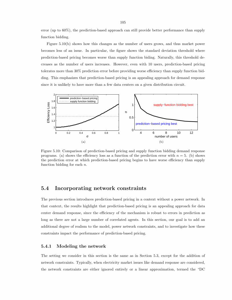
105

error (up to 60%), the prediction-based approach can still provide better performance than supply

function bidding.

Figure 5.10(b) shows how this changes as the number of users grows, and thus market power

becomes less of an issue. In particular, the figure shows the standard deviation threshold where

prediction-based pricing becomes worse than supply function biding. Naturally, this threshold de-

creases as the number of users increases. However, even with 10 users, prediction-based pricing

tolerates more than 30% prediction error before providing worse efficiency than supply function bid-

ding. This emphasizes that prediction-based pricing is an appealing approach for demand response

since it is unlikely to have more than a few data centers on a given distribution circuit.

0 0.2 0.4 0.6 0.8 1

1

1.2

1.4

1.6

1.8

2

σ

Effi

cien

cy L

oss

prediction−based pricingsupply function bidding

(a)

4 6 8 10 120

0.5

1

number of users

σprediction−based pricing best

supply−function bidding best

(b)

Figure 5.10: Comparison of prediction-based pricing and supply function bidding demand responseprograms. (a) shows the efficiency loss as a function of the prediction error with n = 5. (b) showsthe prediction error at which prediction-based pricing begins to have worse efficiency than supplyfunction bidding for each n.

5.4 Incorporating network constraints

The previous section introduces prediction-based pricing in a context without a power network. In

that context, the results highlight that prediction-based pricing is an appealing approach for data

center demand response, since the efficiency of the mechanism is robust to errors in prediction as

long as there are not a large number of correlated agents. In this section, our goal is to add an

additional degree of realism to the model, power network constraints, and to investigate how these

constraints impact the performance of prediction-based pricing.

5.4.1 Modeling the network

The setting we consider in this section is the same as in Section 5.3, except for the addition of

network constraints. Typically, when electricity market issues like demand response are considered,

the network constraints are either ignored entirely or a linear approximation, termed the “DC

106

model,” is used. See [155] for an introduction. However, due to our focus on reducing voltage

violations with data center demand response, the DC model is not appropriate; it assumes the

voltages at all buses are fixed at the reference value, which is seldom true in distribution networks.

As a result, we adopt a different model, called the “branch flow” model, which is commonly used

for modeling distribution systems, e.g., [21, 45]. This model still uses a linear approximation of the

power constraints, but now voltage variations are allowed at all buses except the root bus.

The branch flow model is defined as follows. The power network is represented by a directed,

connected tree G = (N,E), where each node in N := 0, 1, ..., n represent a bus with the root at

bus 0, each edge in E represents a line. Denote an edge by (i, j) or i→ j if it points from bus i to

bus j. The orientation of edges is fixed to be from the root to the leaves for G.

For each edge (i, j) ∈ E, let zij := rij + ixij be the complex impedance on the line, and let

Sij := Pij + iQij be the sending-end complex power from bus i to bus j. This is the same as the

receiving end power since lines are assumed to be lossless.

Let sj = Pj + iQj be the complex net load (load minus generation) on bus j. Here Pj is the

real power consumption, which can be further written as P 0j − sj(p), where P 0

j is the real power

consumption without demand response and sj(p) is the demand reduction given price p. Under our

model, si(p) = Xip,∀i. Qj is the reactive power consumption on bus j and we assume Qj = βjPj ,∀j.

The branch flow model is defined by the following set of power flow equations.

Sij − sj =∑k:j→k

Sjk,∀j, (5.15)

vi − vj = 2Re(z∗ijSij),∀i, j, (5.16)

where Re(·) is the real part of a given complex number. Here (5.15) balances the power on each

bus, and (5.16) characterizes the voltages across line (i, j) according to Ohm’s law.

The constraint for the voltage on each bus is

vi ≤ vi ≤ vi,∀i. (5.17)

5.4.2 Prediction-based pricing in networks

The incorporation of the network has a significant consequence for the design of prediction-based

pricing. Due to the randomness of the cost functions, it is impossible for the voltage constraints

to be always satisfied. This motivates a chance constraint where the goal of the LSE when setting

107

price p is now

E [G(p)] = minp

E [G(p)] (5.18)

s.t. p ≥ 0

Pvoltage violation|p ≤ ε.

To determine more concretely what the set of feasible prices is for the chance constraint above,

we first need to transform the power network constraints into constraints on feasible prices. To

accomplish this, note that (5.15) gives that Sij =∑k∈Tj sk, where Tj is the tree rooted at bus j

(including bus j). Then, we can rewrite (5.16) as

vi − vj = 2Re(z∗ijSij)

= 2Re

(rij − ixij)∑k∈Tj

sk

= 2

rij ∑k∈Tj

Pk + xij∑k∈Tj

Qk

= 2

rij ∑k∈Tj

(P 0k −Xkp

)+ xij

∑k∈Tj

βk(P 0k −Xkp

)= 2

∑k∈Tj

(rij + xijβk)P 0k − 2

∑k∈Tj

(rij + xijβk)Xkp

:= Mij −Nijp.

Note that Mij is a constant here, while Nij is a random variable due to the uncertainties in Xk.

Next, assuming that Ek is the set of edges from root to bus k, we have (using v0 = 1)

vk = 1−∑

(i,j)∈Ek

(Mij −Nijp)

= 1−∑

(i,j)∈Ek

Mij +∑

(i,j)∈Ek

Nijp.

Therefore vk ≤ vk ≤ vk becomes

vk ≤ 1−∑

(i,j)∈Ek

Mij +∑

(i,j)∈Ek

Nijp ≤ vk,

which further implies

vk − 1 +∑

(i,j)∈EkMij∑(i,j)∈Ek Nij

≤ p ≤vk − 1 +

∑(i,j)∈EkMij∑

(i,j)∈Ek Nij.

108

This condition should hold for all buses, and therefore the feasible set is

maxk

vk − 1 +∑

(i,j)∈EkMij∑

(i,j)∈EkNij

≤ p ≤ mink

vk − 1 +∑

(i,j)∈EkMij∑

(i,j)∈EkNij

. (5.19)

We can simplify the feasible set further by assuming that the voltage constraints (5.17) are

satisfied when there is no demand response, i.e.,

vk ≤ 1−∑

(i,j)∈Ek

Mij ≤ vk,∀k. (5.20)

This implies that the feasible range in (5.19) is nonempty.

Additionally, since we only consider demand reduction with p ≥ 0,4 and vk−1+∑

(i,j)∈EkMij ≤

0,∀k, and we assume Xk ≥ 0, we can further simplify the feasible set to

p ≤ mink

vk − 1 +∑

(i,j)∈EkMij∑(i,j)∈Ek Nij

. (5.21)

Again, recall that Nij is random. Therefore, the constraint above is on realizations. Importantly,

for each realization, the constraints are linear, and therefore we can translate the constraints into a

bound on the fraction of violation for each bus as follows.

P

∑(i,j)∈Ek

Nijp ≥ vk − 1 +∑

(i,j)∈Ek

Mij

≤ ε, ∀k. (5.22)

The above equation can be viewed as a concrete specialization of the voltage violation constraint

in (5.18). Note that it has a number of interesting properties. In particular, the violation probability

is a strictly increasing function of p that equals 0 when p = 0 and approaches P∑

(i,j)∈Ek Nij > 0

as p → ∞. Therefore, if P∑

(i,j)∈Ek Nij > 0

is smaller than ε, the chance constraint is satisfied

for all p ≥ 05. Otherwise there is a threshold pε at which point the violation probability exceeds ε.

In this case, the feasible pricing space is [0, pε], and the optimizing price becomes the projection of

the unconstrained price derived in Section 5.3 onto this interval.

5.4.3 The efficiency of prediction-based pricing in networks

The previous analysis highlights that the necessary adjustment in the price used by the LSE due to

network constraints can be achieved via a projection onto a feasible space of prices, which we have

characterized in (5.22). The goal of this section is to understand the impact of network constraints,

i.e., the projection into the feasible space of prices, have on the efficiency of the resulting price.

4Note that all the results here can be easily extended to the case where we allow p to be negative.5This does not happen in our case because we assume Xi’s are positive, therefore P

∑(i,j)∈Ek Nij > 0

= 1

109

The main message of what follows is that network effects do not reduce the efficiency of prediction-

based pricing, when efficiency is measured by the competitive ratio.

In particular, let us compare our algorithm with the clairvoyant algorithm that uses the same fea-

sible set [0, pε] for each realization. This makes the offline algorithm weaker than the one considered

in Section 5.3, i.e., the performance is strictly worse.

Recall that we denote by G(p) and G(p∗(ω)) the cost of our algorithm and the clairvoyant

algorithm in Section 5.3 where network constraints are not considered. Let us now denote by G(pε)

and G(p∗ε (ω)) the cost of our algorithm and the clairvoyant algorithm with the same feasible set

[0, pε], defined as a function of the network constraints.

Our goal is to compare the competitive ratio without network constraints, i.e., E[G(p)]E[G(p∗(ω))] , to the

competitive ratio under network constraints, i.e., E[G(pε)]E[G(p∗ε (ω))] .

The following theorem highlights that constraints on the pricing space actually reduce the ef-

ficiency loss from uncertainty, and so the competitive ratio of prediction-based pricing remains

unchanged when network constraints are considered. In the statement, we consider the feasible

price set R := [p, p] and denote by g(pR) and g(p∗R) the cost of our algorithm and the clairvoyant

algorithm with the same feasible set for a convex function g(·), e.g., a realization of the random

function G(·). Proof is given in Appendix D.5.

Theorem 17. Consider any positive, convex function g(·) that is a realization of the random func-

tion G(·) and any non-empty feasible set R := [p, p]. Then,

g(p)

g(p∗)≥ g(pR)

g(p∗R), (5.23)

and thus

E [G(p)]

E [G(p∗(ω))]≥ E [G(pε)]

E [G(p∗ε (ω))]. (5.24)

A key distinction between this theorem and Theorem 15 is that the feasible price set of both the

optimal and the algorithm are fixed to R := [p, p]. This implies that we are not comparing with the

“true” offline optimal, which may have different feasible sets for the price for different realizations.

Instead, we are comparing with the weaker offline optimal that, because of uncertainty, optimizes

over the same feasible price set as our online algorithm, but then has the foresight necessary to choose

optimally given these price constraints. This is a common choice for comparison when studying the

competitive ratio of online algorithms in situations where clairvoyance yields different feasible action

spaces.

110

5.5 Summary

In this chapter we have highlighted two main points. First, that data center demand response

has significant potential and, second, that prediction-based pricing is an appealing mechanism with

which to extract this potential.

More concretely, we have illustrated that, not only are data centers large loads to target with

demand response programs, they can provide nearly the same degree of flexibility for LSEs as large-

scale storage if properly incentivized. However, this last caveat is crucial – it is much harder to

extract flexibility from data centers than from storage.

To that end, this chapter has argued that prediction-based pricing is a promising market design

for this context. While, in general, prediction-based pricing may be less efficient than supply function

bidding (due to prediction errors), because data centers typically have significant market power on

their distribution networks, supply function bidding can be very inefficient whereas prediction-based

pricing is less influenced.

In particular, the analytic results in Sections 5.3 and 5.4 highlight that the efficiency of prediction-

based pricing is favorable to that of supply function bidding when market power is an issue – even

when predictions are error prone. These analytic results are the first, to our knowledge, that provide

bounds on the competitive ratio of prediction-based pricing programs, and also the first to provide an

analysis of prediction-based pricing programs in a context where network constraints are considered.

111

Chapter 6

Concluding remarks

The coming decades promise explosive growth in the use of renewable energy. For example, while

the current installed capacity of wind power in the U.S. is less than 5% of total generation [58], the

Department of Energy has set a goal to procure 20% of the total generation from wind power by

2030 [56]. This degree of renewable penetration brings with it major challenges for management and

control of the electricity grid as a result of the unpredictable, highly variable nature of renewable

energy sources.

Often, when people think of the challenges for grid management that result from increasing

adoption of renewable energy, the thought is: “if only we had large-scale energy storage...” Large-

scale energy storage, indeed, would solve many of the challenges associated with the unpredictability

and intermittency of wind and solar energy. However, the problem is that large-scale storage is too

expensive, at least for now.

It is this expense that leads to the consideration of demand response as the next-best option.

Demand response (DR) programs seek to provide incentives to induce dynamic management of

customers’ electricity load in response to power supply conditions, for example, reducing their power

consumption in response to a peak load warning signal or request from the utility. The National

Institute of Standards and Technology (NIST) and the Department of Energy (DoE) have both

identified demand response as one of the priority areas for the future smart grid [140, 57]. Further,

the National Assessment of Demand Response Potential report has identified that demand response

has the potential to reduce up to 20% of the total peak electricity demand in the U.S. [66].

In this thesis, we study the dual view of IT and sustainability based on the flexibility of cloud

workloads. The flexibility can come from capacity right-sizing (speed-scaling [185, 165, 19, 40, 163,

59], power-capping [70, 39], moving servers into and out of power saving modes [120, 86, 132, 197,

128]), load shifting (over time [80, 44, 121, 193], geographic load balancing [150, 153, 184, 123, 122,

119, 34, 75, 135]), and even quality degradation [20, 85, 180, 189, 76, 77]. In addition to flexibility

in the workloads, data centers typically have large scale energy storage on-site in order to provide

backup power for their servers [174, 83]. Moreover, they typically also have a backup generator on

112

site in case of extreme failures [125, 79]. Both of these can provide additional opportunities for data

centers to have flexibility in the amount of energy that is drawn from the grid.

Based upon this, we first study how to efficiently incorporate renewable energy into these IT

systems in Chapter 2 and Chapter 3. In order to make broader impacts, our focus switches to data

center demand response in Chapter 4 and Chapter 5 because data centers are particularly well-

suited for participation in demand response programs. To see this, note that, first and foremost,

data centers represent very large loads for the grid. In 2011, they consumed approximately 1.5%

of all electricity worldwide. Some individual data centers can consume up to 50 MW, or more

[79, 78, 160]. Further, the energy consumption of data centers is growing quickly, by approximately

10-12% per year [78, 160, 110]. This growth is crucial for keeping pace with the growth of renewable

adoption predicted for the coming years.

6.1 Opportunities for data center participation in demand

response programs

When illustrating the potential of data center participation in demand response programs in the pre-

vious chapters, we assumed that data centers would adjust their usage (within bounds on flexibility)

exactly the way that the grid operator desired. Of course, this is not what happens in practice.

However, there are many demand response programs available today that allow the grid operator to

extract flexibility from participants through either price signals or direct control signals.

In this section, we summarize some of the most promising opportunities for data center partici-

pation in electricity market and demand response programs that are available today. We divide the

programs into two categories: programs that allow for either “passive” or “active” participation.

By passive participation programs, we mean those where participation does not seek to have direct

impact on the electricity market, as opposed to active participation programs where participation

aims to directly affect the market, e.g., through bidding.

6.1.1 Opportunities for passive participation

Passive programs typically use some sort of “smart” pricing approach. That is, consumers are

encouraged to individually and voluntarily manage their loads through the use of pricing signals.

These programs come in a variety of forms. The following list shows some of the most common in

the U.S.:

1. Time-of-Use Pricing : Certain times during the day are identified as peak, mid-peak, and off-

peak hours, each group having distinct rates for electricity. For example, Portland General

113

Electric Utility has identified 3:00-8:00 PM as peak hours, with peak prices being three times

higher than off-peak prices [149].

2. Inclining Block Rates: Beyond a threshold in the consumer’s monthly, daily, or hourly load,

the price increases to a higher value [156]. This encourages consumers to keep their load below

a certain level at certain times. Inclining block rates are practiced, e.g., by Clatskanie Public

Utility for residential users [47] and by Alabama Power for industrial consumers [15].

3. Peak Pricing : Many utilities also use peak pricing (PP) for large industrial loads, based on

their maximum demand. The maximum demand might be calculated separately for on-peak,

off-peak, or mid-peak hours. For example, Riverside Public Utility calculates the maximum

demand for each on-peak, off-peak, and mid-peak period based on the maximum average

kilowatt input recorded by metering instruments during any 15-minute metered interval in

each month [159].

4. Coincident Peak Pricing : Under coincident peak pricing (CPP), industrial consumers are

charged a very high price (often over 200 times higher than the base rate) for usage during the

coincident peak hour, i.e., the hour when the most electricity is requested from the utility’s

wholesale power supplier. These coincident peaks may typically be accompanied by advance

but short (e.g., 5 minutes) notice, and are often limited to a maximum number of hours per

year. In case of Fort Collins Utilities in Colorado [67, 125], it is common to have about 10 to

12 critical peak warning notices every month.

5. Day-Ahead Pricing : While time-of-use prices are fixed for several months and limited to only

two or three price levels, it is becoming common for many utilities to also offer day-ahead prices

(DAPs) that are calculated based on the clearing market prices in the day-ahead market and

carry a separate price for each hour of the next day. For example, Ameren Illinois Utilities

offer day-ahead prices that are updated daily at 4:30 PM and provide a full table of electricity

prices for each hour during the next day [18].

6. Real-Time Pricing : It some regions, e.g., in Electric Reliability Council of Texas (ERCOT), for

consumers to be charged at real-time prices (RTPs) [60]. Such prices are established every 15

minutes based on the clearing market prices in real-time market. Thus, RTPs are not known

at the time of usage as they are calculated only after-the-fact. This can cause uncertainties to

consumers; however, since RTP charging eliminates the large “insurance premium” that paid

for the luxury of purchasing power at flat or pre-determined rates, it can lead to big savings

for certain consumers.

114

6.1.2 Opportunities for active participation

In contrast to the opportunities for passive participation, which primarily involve responses to price

signals, the market programs we discuss here require active participation in a market via the sub-

mission of bids or negotiation. Programs of this type that are appropriate for data centers fall

into three categories: wholesale electricity markets, ancillary services markets, and load reduction

markets. Each one has multiple participation opportunities, as we explain below.

Wholesale markets

While it is typical for consumers to buy electricity from regional retailers, some independent system

operators (ISOs), such as ERCOT and California ISO, have recently developed a market that allows

consumers to purchase electricity directly from power suppliers by actively participating in one or

both of the following markets. These options offer tremendous flexibility to purchase traditional

and/or green energy to larger costumers, such as data centers.

1. Bilateral markets: A medium or large data center can enter a bilateral contract with a power

supplier to buy electricity or generation rights under mutual agreements. Bilateral contracts

are confidential and flexible. Therefore, data centers can negotiate purchase contracts that

can best fit their energy needs given their load characteristics and load control capabilities.

2. Power markets: A data center may also participate in the wholesale market. A common option

for major load entities is to submit “limit order” bids to the day-ahead market. For each hour

of the day h, such bids indicate that the data center is willing to buy Lh MW electricity at a

price no higher than ph. Once the day-ahead auction is processed, if the market clearing price

at hour h stays below ph, then the data center purchases the rights to the Lh MW of electricity

at hour h and pays the market clearing price. Otherwise, it does not receive the rights to the

Lh MW of electricity at hour h and must purchase needed energy in the real-time market at

“unknown prices”.

Ancillary Service markets

Another opportunity that is well-suited to data centers is to participate in ancillary service markets

as a “load resource”. In fact, many of the existing ancillary service markets, e.g., PJM and ERCOT,

allow providing a portion (e.g., 20%, in case of PJM) of their ancillary services from load resources.

Ancillary services are defined as the services necessary to support the transmission of energy to loads

while maintaining reliable operation and security of the electricity transmission system.

Balancing supply and demand can be achieved by either adjusting generation or adjusting con-

sumption. Therefore, payments for load reductions to load resources are equal, dollar for dollar, to

that which suppliers are paid for increasing generation. In fact, similar to generators, the “value” of

115

a load resource (e.g., a large data center) depends on three factors: (i) how quickly it can respond

to change (reduce or increase) its load; (ii) the cost at which a load resource is willing to adjust its

load; and (iii) the market condition at which the service was offered. Accordingly, there are different

ancillary services that could be offered by load resources based on their capabilities. In PJM and

ERCOT, such services differ in response time and are as follows [60, 147]:

1. Spinning reserves: In this service, a command to interrupt or reduce the load comes either

from an on-site under-frequency relay (UFR) or through a (10 minutes-ahead or shorter)

notice signal from the ISO. The load resource is then required to provide holding service for

at least 15 minutes and up to multiple hours. The spinning reserve service is also referred to

as “responsive reserve service”.

2. Non-spinning reserves: Non-spinning reserves provide the same service as spinning reserves,

but are not required to respond to notices as quickly, i.e., signals arrive with 30-minutes notice

typically.

3. Regulation services: When offering regulation service, a flexible load (such as data center) needs

to respond to up/down signals that arrive, e.g., every 4 or 10 seconds, by decreasing/increasing

the load accordingly, while meeting rigorous performance monitoring criteria. Regulation can

be done at different resolutions. For example, in PJM, there are two, Reg A (traditional) and

Reg D (dynamic), regulation signals [147]. Reg D command signals fluctuate more severely.

Accordingly, there is a higher payment for offering dynamic regulation.

In general, making decisions to offer ancillary service is very difficult. However, if it is done properly,

it has the potential to bring major financial benefits to data centers, in addition to helping the grid.

To be qualified as a load resource, a data center must (i) meet a minimum flexible load capacity

(e.g., 1 MW in ERCOT), (ii) install real-time telemetry systems, and (iii) pass and maintain high

scores in “performance tests”.

The payments for participation in such programs are quite complicated. We give a brief overview

in the following.

1. Load resource payments: Load resources that offer ancillary services typically receive two

types of payments. The first payment is the “capacity payment”, which is made simply for

being available. The second payment is the “operation payment”, which is made only if the

service was actually called. For the responsive and non-spinning reserves, this payment is

typically calculated based on the locational marginal price (LMP) at the power grid bus where

the load resource is located. For regulation services, additional payments are made based

on “mileage” for each regulation signal type [147], which is combined with several factors

such as LMP, “benefit factor” (that indicates the scarcity of load and generation resources

116

to perform regulation), “historical performance score” of the load resource, and the total

regulation capacity that is offered by the load resource.

2. Performance evaluation: While assessing the performance of reserve services is typically simple,

the performance evaluation for regulation services requires advanced monitoring and analysis.

For example, PJM evaluates regulation performance based on scores on “delay”, “correlation”,

and “precision” [148]. The Delay Score quantifies the delay between the regulation signal and

changes in demand. The Correlation Score measures the accuracy in matching the regulation

signal, using the correlation between regulation and response signals. The Precision Score is

calculated as an hourly average of the difference between the regulation and response signals

over 10 seconds sampling intervals. The final performance score is calculated as a weighted

summation of all three scores. Maintaining a minimum (e.g., 75%) score is needed to stay

qualified to offer regulation services.

3. Bidding process: The bids for offering ancillary services are submitted to ancillary service mar-

kets. Various information must be included in the bid. For example, for regulation services,

the capacity and the regulation type (traditional or dynamic) should be indicated. The finan-

cial element of the bid could be “cost-based” or “price-based”. The former parameterizes the

service cost function, e.g., in terms of start-up and incremental costs for local generators. The

latter is in the form of price schedules that indicate the price of offering the service at each

time of operation.

Voluntary Load Reduction

A third option well-suited for data centers is to offer some voluntary services to regional grid oper-

ators. For example, in ERCOT, industrial consumers can offer “voluntary load reduction” services

to regional operators, called Qualified Scheduling Entities (QSEs). There are at least two key dis-

tinctions between offering load reduction to QSEs and offering ancillary services to ISOs that lead

to important differences for data center management. First, such services are voluntary and usually

guarantee only best-effort services, thus participation carries little or no risk. In turn, they typically

have lower payments. Second, they do not require bidding and have flexible contracts. Thus, a

potential load resource such as data center will need to negotiate with its corresponding QSE to

settle down the terms of the contract.

117

6.2 Challenges that limit data center participation in de-

mand response

The previous sections have highlighted the potential for data center demand response and the op-

portunities data centers have for participation. It is important to emphasize that data center par-

ticipation in demand response programs truly has the potential to be a “win-win”: data centers

provide a significant service to grid operators and demand response programs provide a significant

revenue source for data centers.

However, despite this potential “win-win” opportunity, data centers today are largely non-

participants in the demand response programs we discuss above. The reasons for this are not

mysterious. There are a number of significant challenges that lead to this unfortunate fact. Below,

we outline some of these biggest reasons. Then, in the next section, we discuss recent research

progress in the academic and industrial research communities that is beginning to alleviate these

challenges.

Challenge 1: Regulation and market maturity

First and foremost, it is important to emphasize that, though we have outlined a large number of

participation opportunities for data centers in demand response programs, many of these programs

are not available to data centers in markets today. While some utilities have been quick to move to

adjust regulations to allow greater participation in market programs, many have been quite slow.

As a result, in any given area, the opportunities for data center demand response participation may

be limited to simple, traditional smart pricing programs such as coincident peak pricing which, as

we discuss next, are not well-suited for the risk tolerance of data centers.

Challenge 2: Risk management

Data centers are typically in the business of maximizing uptime and performance, and energy issues

are certainly secondary to maintaining strong guarantees about these primary measures. However,

participation in demand response programs always comes with some risk. This risk may be purely fi-

nancial, e.g., in passive participation programs, or it may have the possibility of uptime/performance

degradations, e.g., in active participation programs. As a result, risk management is a crucial issue

for data center participation in demand response programs. Taking a huge financial/performance

hit because the grid sends a price/control signal at the same point when the data center is heavily

loaded is a serious concern that limits data center participation in current market programs. In fact,

for exactly this reason, data centers prefer to negotiate long term energy contracts with fixed usage

prices.

118

Challenge 3: Who has control?

An active debate within the demand response field is that of who should have control? Grid operators

would like to have a guaranteed response when they ask for it; which leads to “direct load control”

programs for which the grid sends a signal to a controller of the program participant. However, of

course, this is not always acceptable to participants. In particular, such programs are inappropriate

for data centers given the risk management issues discussed above. The other extreme alternative

is “prices-to-devices” where real-time prices are conveyed to participants; however such programs

typically require huge price variation in order to extract desired responses. Again, this volatility is

not acceptable given the risk tolerance of data centers. Thus, other programs must be developed in

order to facilitate data center participation.

Challenge 4: Market complexity

Financially, the active participation programs we have described have a huge potential for data

centers. However, as we have discussed, participation in these programs is highly regulated and

the bidding necessary to extract profits is something that is typically difficult to automate and

incorporate into a data center management system. This complexity has, to this point, prevented

data centers from entering these markets despite the financial opportunities.

Challenge 5: Market power

The challenges that we have outlined so far relate to data center participation. However, there are

also significant challenges on the grid operator side. One that is particularly salient is the potential

for data centers to manipulate market prices. In particular, as we have discussed, data centers

are very large loads. They can make up 20-50% of the load on their distribution circuit. In such

situations, if they participate aggressively in some of these market programs there is a significant

potential for them to wield market power to manipulate prices in their favor. Given that many of

these markets have been designed for situations in which many small loads all act as price-takers,

grid operators are rightfully nervous about loosening regulations to allow data center participation.

6.3 Recent progress in data center demand response

Given the challenges that remain before data center demand response participation can realize its

potential, there are clearly many important research questions to address. To that end, a new

field is emerging at the intersection of data center management and power systems that focuses

on facilitating the interaction of data centers in demand response programs. In the following, we

summarize some of the progress that has been made toward addressing the challenges we outlined

119

in the previous section. Note that, though progress has been made, it is clear that many, significant

challenges are yet to be addressed.

We organize the progress made to this point into two categories: (i) progress toward the im-

proved management of data centers to facilitate participation in demand response programs; and

(ii) progress toward the design of new market programs that are appropriate for data center partic-

ipation.

6.3.1 Managing data center participation in demand response

The task of managing data center participation in a demand response program is clearly a difficult

one; however, because of the large literature on energy-efficient data centers that has emerged

over the past decade, there are many tools that have already been well-developed at this point.

In particular, techniques for right-sizing, load shifting, quality degradation, etc., are developed

and, sometimes, used in practice already. However, the challenge of how to use them to optimize

participation in demand response programs is still unsolved.

In particular, different demand response markets require very different strategies. Classically,

much of the academic work on energy-efficient data centers has focused on time-of-use pricing, and

so there are many strategies available for such programs, e.g., [103, 108, 130, 117, 70, 44, 120, 86,

132, 197, 193, 121]. The algorithmic challenges in such designs often stem from the unpredictability

of workload and the costs associated with switching the state of servers.

More generally though, there are many other options for demand response programs which can

provide significantly larger financial incentives for data centers. For example, it is often beneficial for

data centers to hedge long-term energy contracts with participation in spot-markets, thus creating

a challenging online, multi-time scale optimization problem. Designs have started to emerge for

optimizing such contracts [154, 139, 152, 54, 55, 195].

Another popular option for demand response is coincident peak pricing programs. Such programs

provide a challenge for data center management since there is significant uncertainty about when

coincident peak warnings will be sent to the data center, thus signaling a reduction. Recent work has

looked at using online, robust optimization as a tool for managing participation in such programs

[109, 164, 35, 125, 178].

The programs we have discussed so far are all passive. Participation in active demand response

programs is much more challenging, and has only recently begun to be studied. For example, recent

papers have looked at managing data center participation in regulation markets and ancillary service

markets [37, 74, 38, 39, 12, 12, 13].

In addition to the details of the particular program, there are key challenges that demand response

can create within data centers. For example, many data centers are multi-tenant, i.e., they rent space

to many different tenants. In such situations, the data center operator does not have control over

120

the computing resources and so when a demand response signal is received, it cannot manage the

response directly and must find a way to encourage the tenants to respond appropriately. Some

recent work has looked at designing mechanisms for this setting [158].

Another level of complexity on top of all the issues we have discussed so far is the fact that

data centers often have local resources such as energy storage, renewable energy, and/or backup

generators on-site. Each of these adds additional uncertainty and complexity to the participation

decisions discussed above, and each has been studied by recent work [125, 169, 127, 75, 76, 174].

6.3.2 Design of market programs appropriate for data centers

While significant progress has been made on developing tools and algorithms to facilitate data centers

participation in demand response programs, it is clear that, in the long term, the development of

new market programs are crucial to efficiently extract data centers flexibility. However, it is not at

all clear yet what form these new market programs should take.

There are multiple tradeoffs at play in the design of new market programs. Should the new

programs be passive or active? How much control should the load serving entity wield versus the

data center? What time-scale should data centers be encouraged to provide flexibility over? These

and many other questions are at the heart of the emerging research on market designs for data center

demand response.

One key issue that has emerged as crucial in the design of new market programs is the market

power that data centers wield. As we have already highlighted, data centers can make up a significant

proportion of the load on a given distribution circuit, and thus they have the potential to significantly

manipulate prices if care is not taken in design.

This worry is particularly salient given the typical “price-taker” assumption that goes into the

design of most demand response programs. Clearly data centers need not be price-takers. However,

quantifying the potential for market power is a difficult task, and only recently have market power

metrics that incorporate transmission constraints begun to emerge [33, 186, 116, 190]. Noticeably,

none of these metrics are designed for assessing market power on distribution networks.

Thus, there seems to be a tradeoff between pricing approaches and bid-based approaches in

terms of market power versus prediction error. Specifically, bid-based approaches generally suffer if a

participant has market power, e.g., [181, 105, 191], while pricing-based approaches require predicting

the flexibility of participants in order to set prices efficiently, e.g., [182, 48, 136, 84, 118]. To this

point, it is not yet clear which is more appropriate for data center demand response programs.

Finally, the above discussion has focused entirely on a single data center. To this point, there

are no existing demand response programs that are designed to extract geographic flexibility. Such

programs could be of crucial importance in areas where large-scale solar installations stress circuits

across different regions in a load serving entity [134, 179].

121

6.4 Future directions

Regarding geographical load balancing, while we have more recent results about online algorithms

for geographical load balancing [119], there are a number of interesting directions for future work.

With respect to the design of distributed algorithms, one aspect that our model has ignored is the

switching cost (in terms of delay and wear-and-tear) associated with switching servers into and out

of power-saving modes. Our model also ignores issues related to reliability and availability, which

are quite important in practice. With respect to the social impact of geographical load balancing,

our results highlight the opportunity provided by geographical load balancing for demand response;

however, there are many issues left to be considered. For example, which demand response market

should Internet-scale systems participate in to minimize costs? How can policy decisions such as

cap-and-trade be used to provide the proper incentives for Internet-scale systems, such as [114]?

Can Internet-scale systems use energy storage at data centers in order to magnify cost reductions

when participating in demand response markets? Answering these questions will pave the way for

greener geographic load balancing.

For data center demand response, in particular, an interesting direction is to adapt the algorithms

presented in Chapter 4 in order to incorporate energy storage at the data center. More generally,

Internet-scale systems are typically provided by a geographically distributed data centers, and so it

would be interesting to understand how the “geographical load balancing” performed by such sys-

tems interacts with coincident peak pricing. This “moving bits, not watts” scheme can significantly

reduce local power network pressure without adding further load to the (possibly already) congested

transmission network. Additionally, CPP programs are just one example of demand response pro-

grams. Though CPP programs are currently the most common form of demand response program,

a number of new programs are emerging. It is important to understand how each of these programs,

e.g., [12], interact with data center planning.

Much work still remains before prediction-based pricing studied in Chapter 5 can be used in

practice. In particular, in this chapter we have adopted quadratic objectives, and it is important to

understand the impact of this. For example, in the context of internet congestion management, [126]

has studied the impact of convexity of costs on the contrast between time-of-use pricing and fixed-

budget rebates. A similar study in the context of predictive pricing and supply function bidding is

crucial.

Further, it is important to do an empirical study to understand how predictable the response

of data centers will be in demand response programs. Initial pilot studies along these lines are

proceeding in some demand response markets, but these have yet to focus on data centers specifically.

Depending on the result of such studies, it may be natural to consider hybrid mechanisms that

combine predictions and bidding in order to extract supply function information from data centers.

122

Additionally, many practical aspects of prediction-based pricing programs still require careful

thought. For example, what is the appropriate time-scale at which prices should be adjusted? The

time-scale chosen allows for a balance between the responsiveness desired by the LSE and the risk-

aversion of the data center. Further, in this chapter we have assumed a scalar price. One could

also investigate location dependent prices in distribution networks, similar to locational marginal

prices (LMPs) for transmission networks. While these are not currently used, the extra geographical

flexibility they provide could be valuable. Finally, there are interesting exploration-exploitation

tradeoffs that come up when setting prices in prediction-based pricing programs. We have not

addressed this issue in this thesis due to the complexities of the power network, but work in the

operations research community has begun to study this in other contexts [27, 28], using “regret” as

the performance measure. It would be interesting for future work to incorporate this issue into the

demand response context.

123

Bibliography

[1] www.enernoc.com.

[2] http://perspectives.mvdirona.com/2009/10/31/TheCostOfLatency.aspx.

[3] Kvm kernel based virtual machine. http://www.redhat.com/f/pdf/rhev/DOC-KVM.pdf.

[4] Sysbench: a system performance benchmark. http://sysbench.sourceforge.net/.

[5] US Census Bureau, http://www.census.gov.

[6] Webair and enernoc turn data centers into virtual power plants through de-

mand response. http://blog.webair.com/webair-and-enernoc-turn-data-centers-into-virtual-

power-plants-through-demand-response/93/.

[7] Electricity Energy Storage Technology Options: A White Paper Primer on Applications, Costs

and Benefits. 2010.

[8] Server and data center energy efficiency, Final Report to Congress, U.S. Environmental Pro-

tection Agency, 2007.

[9] Clean urban energy: Turn buildings into batteries. http://www.cleanurbanenergy.com/assets/documents/Turning

Buildings into Batteries.pdf, 2011.

[10] V. K. Adhikari, S. Jain, and Z.-L. Zhang. YouTube traffic dynamics and its interplay with a

tier-1 ISP: An ISP perspective. In Proc. ACM IMC, pages 431–443, 2010.

[11] D. J. Aigner and J. G. Hirschberg. Commercial/industrial customer response to time-of-use

electricity prices: Some experimental results. The RAND Journal of Economics, 16(3):341–

355, 1985.

[12] D. Aikema, R. Simmonds, and H. Zareipour. Data centres in the ancillary services market. In

Green Computing Conference (IGCC), 2012 International, pages 1–10. IEEE, 2012.

[13] B. Aksanli and T. Rosing. Providing regulation services and managing data center peak

power budgets. In Proc. of the IEEE Design, Automation and Test in Europe Conference and

Exhibition, Dresden, Germany, March 2014.

124

[14] B. Aksanli, J. Venkatesh, L. Zhang, and T. Rosing. Utilizing green energy prediction to

schedule mixed batch and service jobs in data centers. ACM SIGOPS Operating Systems

Review, 45(3):53–57, 2012.

[15] Alabama Power - A Southern Company. Incemental Load Pricing.

http://www.alabamapower.com/business/pricing-rates/pdf/ILD.pdf, April 2011.

[16] S. Albers. Energy-efficient algorithms. Comm. of the ACM, 53(5):86–96, 2010.

[17] B. Allaz and J. Vila. Cournot competition, forward markets and efficiency. Journal of Eco-

nomic Theory, 59(1):1–16, 1993.

[18] Ameren Energy. Day-ahead and Real Time Electricity Prices.

https://www2.ameren.com/RetailEnergy/realtimeprices.aspx, December 2012.

[19] L. L. H. Andrew, M. Lin, and A. Wierman. Optimality, fairness and robustness in speed

scaling designs. In Proc. ACM SIGMETRICS, 2010.

[20] W. Baek and T. M. Chilimbi. Green: a framework for supporting energy-conscious program-

ming using controlled approximation. In ACM Sigplan Notices, volume 45, pages 198–209.

ACM, 2010.

[21] M. Baran and F. F. Wu. Optimal sizing of capacitors placed on a radial distribution system.

IEEE Transactions on Power Delivery, 4(1):735–743, 1989.

[22] L. Barroso and U. Holzle. The datacenter as a computer: An introduction to the design of

warehouse-scale machines. Synthesis Lectures on Computer Architecture, 4(1):1–108, 2009.

[23] C. E. Bash, C. D. Patel, , and R. K. Sharma. Dynamic thermal management of aircooled data

centers. In Proc. of ITHERM, 2006.

[24] A. Beloglazov, R. Buyya, Y. C. Lee, A. Zomaya, et al. A taxonomy and survey of energy-

efficient data centers and cloud computing systems. Advances in Computers, 82(2):47–111,

2011.

[25] D. P. Bertsekas. Nonlinear Programming. Athena Scientific, 1999.

[26] D. P. Bertsekas and J. N. Tsitsiklis. Parallel and Distributed Computation: Numerical Methods.

Athena Scientific, 1989.

[27] O. Besbes and A. Zeevi. Dynamic pricing without knowing the demand function: Risk bounds

and near-optimal algorithms. Operations Research, 57(6):1407–1420, 2009.

[28] O. Besbes and A. Zeevi. On the minimax complexity of pricing in a changing environment.

Operations research, 59(1):66–79, 2011.

125

[29] S. Blagodurov, D. Gmach, M. Arlitt, Y. Chen, C. Hyser, and A. Fedorova. Maximizing server

utilization while meeting critical slas via weight-based collocation management. In Proc. of

IM, 2013.

[30] F. Bleier. Fan Handbook: Selection, Application and Design. New York: McGraw-Hill, 1997.

[31] S. Boyd and L. Vandenberghe. Convex Optimization. Cambridge University Press, 2004.

[32] T. Breen, E. Walsh, J. Punch, C. Bash, and A. Shah. From chip to cooling tower data center

modeling: Influence of server inlet temperature and temperature rise across cabinet. Journal

of Electronic Packaging, 133.

[33] D. W. Cai and A. Wierman. Inefficiency in forward markets with supply friction. In Proc. of

IEEE CDC, 2013.

[34] J. Camacho, Y. Zhang, M. Chen, and D. Chiu. Balance your bids before your bits: The

economics of geographic load-balancing. In Proc. of ACM e-Energy, 2014.

[35] P. Cappers, C. Goldman, and D. Kathan. Demand response in us electricity markets: Empirical

evidence. Energy, 35(4):1526–1535, 2010.

[36] S. Carley. State renewable energy electricity policies: An empirical evaluation of effectiveness.

Energy Policy, 37(8):3071–3081, Aug 2009.

[37] H. Chen, M. Caramanis, and A. K. Coskun. The data center as a grid load stabilizer. Pro-

ceedings of the Asia and South Pacific Design Automation Conference (ASP-DAC), 2014.

[38] H. Chen, A. K. Coskun, and M. C. Caramanis. Real-time power control of data centers for

providing regulation service. Proc. 52nd CDC, 2013.

[39] H. Chen, C. Hankendi, M. C. Caramanis, and A. K. Coskun. Dynamic server power capping

for enabling data center participation in power markets. In Proceedings of the International

Conference on Computer-Aided Design, pages 122–129. IEEE Press, 2013.

[40] L. Chen, N. Li, and S. H. Low. On the interaction between load balancing and speed scaling.

In ITA Workshop, 2011.

[41] L. Chen, N. Li, S. H. Low, and J. C. Doyle. Two market models for demand response in power

networks. In IEEE SmartGridComm, pages 397–402, 2010.

[42] Y. Chen, S. Alspaugh, and R. Katz. Interactive analytical processing in big data systems: a

cross-industry study of mapreduce workloads. Proc. of VLDB, 2012.

[43] Y. Chen, A. Das, W. Qin, A. Sivasubramaniam, Q. Wang, and N. Gautam. Managing server

energy and operational costs in hosting centers. In Proc. ACM SIGMETRICS, 2005.

126

[44] Y. Chen, D. Gmach, C. Hyser, Z. Wang, C. Bash, C. Hoover, and S. Singhal. Integrated

management of application performance, power and cooling in data centers. In Proc. of NOMS,

2010.

[45] H.-D. Chiang and M. E. Baran. On the existence and uniqueness of load flow solution for

radial distribution power networks. IEEE Transactions on Circuits and Systems, 37(3):410–

416, 1990.

[46] J. Choi, S. Govindan, B. Urgaonkar, and A. Sivasubramaniam. Profiling, prediction, and

capping of power consumption in consolidated environments. In MASCOTS, 2008.

[47] Clatskanie People Utility District. Rate Schedules Summary.

http://www.clatskaniepud.com/Rate Schedules.htm, June 2012.

[48] A. J. Conejo, J. M. Morales, and L. Baringo. Real-time demand response model. IEEE

Transactions on Smart Grid, 1(3):236–242, 2010.

[49] M. Conti and C. Nazionale. Load distribution among replicated web servers: A QoS-based

approach. In Proc. ACM WISP, pages 12–19, 1999.

[50] G. Cook. How clean is your cloud, 2012.

[51] D. R. Cox. Prediction by exponentially weighted moving averages and related methods, 1961.

[52] A. Croll and S. Power. How web speed affects online business KPIs.

http://www.watchingwebsites.com, 2009.

[53] N. Deng, C. Stewart, J. Kelley, D. Gmach, and M. Arlitt. Adaptive green hosting. In Pro-

ceedings of ICAC, 2012.

[54] W. Deng, F. Liu, H. Jin, and C. Wu. Smartdpss: cost-minimizing multi-source power supply

for datacenters with arbitrary demand. In Distributed Computing Systems (ICDCS), 2013

IEEE 33rd International Conference on, pages 420–429. IEEE, 2013.

[55] W. Deng, F. Liu, H. Jin, C. Wu, and X. Liu. Multigreen: cost-minimizing multi-source data-

center power supply with online control. In Proceedings of the fourth international conference

on Future energy systems, pages 149–160. ACM, 2013.

[56] Department of Energy. 20% wind energy by 2030. http://www.20percentwind.org/.

[57] Department of Energy. The smart grid: an introduction, 2008. http://energy.gov.

[58] Department of Energy. Installed wind capacity. http://www.windpoweringamerica.gov/wind installed

capacity.asp, June 2012.

127

[59] M. Elahi, C. Williamson, and P. Woelfel. Decoupled speed scaling: Analysis and evaluation.

Performance Evaluation, 2013.

[60] Electric Reliability Council of Texas. Load Participation in the ERCOT Nodal Market. Pre-

pared by the Demand-Side Working Group of the ERCOT Wholesale Market Subcommittee,

Version N 1.0, June 2007.

[61] EPA. US Emission Standards for Nonroad Diesel Engines.

www.dieselnet.com/standards/us/nonroad.php.

[62] X. Fan, W.-D. Weber, and L. A. Barroso. Power provisioning for a warehouse-sized computer.

In Proc. ISCA, 2007.

[63] X. Fang, S. Misra, G. Xue, and D. Yang. Smart grid: the new and improved power grid: a

survey. Communications Surveys & Tutorials, IEEE, 14(4):944–980, 2012.

[64] M. Farivar, C. R. Clarke, S. H. Low, and K. M. Chandy. Inverter var control for distribution

systems with renewables. In IEEE SmartGridComm, pages 457–462, 2011.

[65] M. Farivar, R. Neal, C. Clarke, and S. Low. Optimal inverter var control in distribution

systems with high pv penetration. In IEEE Power and Energy Society General Meeting, pages

1–7, 2012.

[66] Federal Energy Regulatory Commission. National assessment of demand response potential.

http://www.ferc.gov/legal/staff-reports/06-09-demand-response.pdf, June 2009.

[67] Fort Collins Utilities. Coincident Peak. http://www.fcgov.com/utilities/business/rates/electric/coincident-

peak, 2012.

[68] L. Gan, U. Topcu, and S. H. Low. Optimal decentralized protocol for electric vehicle charging.

In IEEE CDC, pages 5798–5804, 2011.

[69] L. Gan, A. Wierman, U. Topcu, N. Chen, and S. H. Low. Real-time deferrable load control:

handling the uncertainties of renewable generation. In Proc. of ACM eEnergy, pages 113–124,

2013.

[70] A. Gandhi, Y. Chen, D. Gmach, M. Arlitt, and M. Marwah. Minimizing data center SLA

violations and power consumption via hybrid resource provisioning. In Proc. of IGCC, 2011.

[71] A. Gandhi, M. Harchol-Balter, and C. L. R. Das. Optimal power allocation in server farms.

In Proc. of ACM Sigmetrics, 2009.

[72] P. X. Gao, A. R. Curtis, B. Wong, and S. Keshav. It’s not easy being green. In Proc. of ACM

SIGCOMM 2012.

128

[73] N. Gast, J.-Y. Le Boudec, A. Proutiere, and D.-C. Tomozei. Impact of storage on the efficiency

and prices in real-time electricity markets. In Proceedings of the fourth international conference

on Future energy systems, pages 15–26. ACM, 2013.

[74] M. Ghamkhari and H. Mohsenian-Rad. Data centers to offer ancillary services. In Proc. of the

IEEE International Conference on Smart Grid Communications (SmartGridComm), 2012.

[75] M. Ghamkhari and H. Mohsenian-Rad. Optimal integration of renewable energy resources

in data centers with behind-the-meter renewable generator. In Proc. of IEEE International

Conference on Communications (ICC), 2012.

[76] M. Ghamkhari and H. Mohsenian-Rad. Energy and performance management of green data

centers: a profit maximization approach. IEEE Trans. on Smart Grid, 4(2):1017–1025, 2013.

[77] M. Ghamkhari and H. Mohsenian-Rad. Profit maximization and power management of green

data centers supporting multiple slas. In Proc. of IEEE International Conference on Comput-

ing, Networking and Communications (ICNC), 2013.

[78] G. Ghatikar, V. Ganti, N. Matson, and M. Piette. Demand response opportunities and enabling

technologies for data centers: Findings from field studies. 2012.

[79] J. Glanz. Power, pollution and the internet. New York Times, 2012.

[80] D. Gmach, J. Rolia, C. Bash, Y. Chen, T. Christian, A. Shah, R. Sharma, and Z. Wang.

Capacity planning and power management to exploit sustainable energy. In Proc. of CNSM,

2010.

[81] I. Goiri, K. Le, T. D. Nguyen, J. Guitart, J. Torres, and R. Bianchini. Greenhadoop: Lever-

aging green energy in data-processing frameworks. In Eurosys, 2012.

[82] S. Govindan, J. Choi, B. Urgaonkar, A. Sivasubramaniam, and A. Baldini. Statistical profiling-

based techniques for effective power provisioning in data centers. In Proc. of EuroSys, 2009.

[83] S. Govindan, D. Wang, A. Sivasubramaniam, and B. Urgaonkar. Aggressive datacenter power

provisioning with batteries. ACM Transactions on Computer Systems (TOCS), 31(1):2, 2013.

[84] H. Mohsenian-Rad, V. Wong, J. Jatskevich, R. Schober, and A. Leon-Garcia. Autonomous

Demand Side Management Based on Game-Theoretic Energy Consumption Scheduling for the

Future Smart Grid. IEEE Transactions on Smart Grid, 1(3):320–331, December 2010.

[85] Y. He, S. Elnikety, J. Larus, and C. Yan. Zeta: scheduling interactive services with partial

execution. In Proceedings of the Third ACM Symposium on Cloud Computing, page 12. ACM,

2012.

129

[86] J. Heo, P. Jayachandran, I. Shin, D. Wang, T. Abdelzaher, and X. Liu. Optituner: On perfor-

mance composition and server farm energy minimization application. Parallel and Distributed

Systems, IEEE Transactions on, 22(11):1871–1878, 2011.

[87] J. Holman. Heat Transfer. 8th ed. New York: McGraw-Hill, 1997.

[88] Y.-Y. Hsu and C.-C. Su. Dispatch of direct load control using dynamic programming. IEEE

Transactions on Power Systems, 6(3):1056–1061, 1991.

[89] http://cvxr.com/cvx/.

[90] http://rredc.nrel.gov. 2010.

[91] https://www.sce.com/wps/portal/home/regulatory/load-profiles.

[92] http://wind.nrel.gov. 2010.

[93] http://www.apple.com/environment/renewable-energy.

[94] http://www.datacenterknowledge.com, 2008.

[95] http://www.eia.doe.gov.

[96] http://www.ferc.gov/market-oversight/mkt electric.

[97] http://www.google.com/green/energy/.

[98] http://www.hpl.hp.com/research/linux/httperf/.

[99] http://www.nrel.gov/midc/lmu/.

[100] L. Huang, J. Walrand, and K. Ramchandran. Optimal demand response with energy storage

management. In IEEE SmartGridComm, pages 61–66, 2012.

[101] W. Huang, M. Allen-Ware, J. Carter, E. Elnozahy, H. Hamann, T. Keller, C. Lefurgy, J. Li,

and J. R. Karthick Rajamani. Tapo: Thermal-aware power optimization techniques for servers

and data centers. In Proc. of IGCC, 2011.

[102] S. Irani and K. R. Pruhs. Algorithmic problems in power management. SIGACT News,

36(2):63–76, 2005.

[103] D. Irwin, N. Sharma, and P. Shenoy. Towards continuous policy-driven demand response in

data centers. Computer Communication Review, 41(4), 2011.

[104] B. U. Jeonghwan Choi, Sriram Govindan and A. Sivasubramaniam. Power consumption pre-

diction and power-aware packing in consolidated environments. IEEE Transactions on Com-

puters, 59(12), 2010.

130

[105] R. Johari and J. N. Tsitsiklis. Parameterized supply function bidding: Equilibrium and effi-

ciency. Operations research, 59(5):1079–1089, 2011.

[106] A. Kansal, J. Hsu, S. Zahedi, and M. B. Srivastava. Power management in energy harvesting

sensor networks, 2007.

[107] S. Kaxiras and M. Martonosi. Computer Architecture Techniques for Power-Efficiency. Morgan

& Claypool, 2008.

[108] C. Kelly, A. Ruzzelli, and E. Mangina. Using electricity market analytics to reduce cost and

environmental impact. In Green Technologies Conference, 2013 IEEE, pages 414–421. IEEE,

2013.

[109] S. Kiliccote, M. A. Piette, and D. Hansen. Advanced controls and communications for demand

response and energy efficiency in commercial buildings. 2006.

[110] J. Koomey. Growth in data center electricity use 2005 to 2010. Oakland, CA, Analytics Press,

http://www.analyticspress.com/datacenters.html.

[111] R. Krishnan, H. V. Madhyastha, S. Srinivasan, S. Jain, A. Krishnamurthy, T. Anderson, and

J. Gao. Moving beyond end-to-end path information to optimize CDN performance. In Proc.

ACM Sigcomm, 2009.

[112] K. Le, R. Bianchini, M. Martonosi, and T. Nguyen. Cost-and energy-aware load distribution

across data centers. Proceedings of HotPower, 2009.

[113] K. Le, R. Bianchini, J. Zhang, Y. Jaluria, J. Meng, and T. D. Nguyen. Reducing electricity

cost through virtual machine placement in high performance computing clouds. In Proceedings

of 2011 International Conference for High Performance Computing, Networking, Storage and

Analysis, page 22. ACM, 2011.

[114] K. Le, O. Bilgir, R. Bianchini, M. Martonosi, and T. D. Nguyen. Capping the brown energy

consumption of internet services at low cost. In Proc. IGCC, 2010.

[115] J.-Y. Le Boudec and D.-C. Tomozei. A demand-response calculus with perfect batteries. In

Measurement, Modelling, and Evaluation of Computing Systems and Dependability and Fault

Tolerance, pages 273–287. Springer Berlin Heidelberg, 2012.

[116] Y. Y. Lee, R. Baldick, and J. Hur. Firm-based measurements of market power in transmission-

constrained electricity markets. IEEE Transactions on Power Systems, 26(4):1962–1970, Nov.

2011.

131

[117] J. Li, Z. Li, K. Ren, and X. Liu. Towards optimal electric demand management for internet

data centers. Smart Grid, IEEE Transactions on, 3(1):183–192, 2012.

[118] N. Li, L. Chen, and S. H. Low. Optimal demand response based on utility maximization in

power networks. In IEEE Power and Energy Society General Meeting, pages 1–8, 2011.

[119] M. Lin, Z. Liu, A. Wierman, and L. L. Andrew. Online algorithms for geographical load

balancing. In Proc. of IGCC, 2012.

[120] M. Lin, A. Wierman, L. L. H. Andrew, and E. Thereska. Dynamic right-sizing for power-

proportional data centers. In Proc. IEEE INFOCOM, 2011.

[121] Z. Liu, Y. Chen, C. Bash, A. Wierman, D. Gmach, Z. Wang, M. Marwah, and C. Hyser.

Renewable and cooling aware workload management for sustainable data centers. In Proc.

ACM SIGMETRICS 2012, volume 40, pages 175–186. ACM, 2012.

[122] Z. Liu, M. Lin, A. Wierman, S. Low, and L. Andrew. Geographical load balancing with

renewables. ACM SIGMETRICS Performance Evaluation Review, 39(3):62–66, 2011.

[123] Z. Liu, M. Lin, A. Wierman, S. H. Low, and L. L. H. Andrew. Greening geographical load

balancing. In Proc. ACM Sigmetrics, 2011.

[124] Z. Liu, I. Liu, S. Low, and A. Wierman. Pricing data center demand response. In Proc. ACM

Sigmetrics, 2014.

[125] Z. Liu, A. Wierman, Y. Chen, B. Razon, and N. Chen. Data center demand response: Avoid-

ing the coincident peak via workload shifting and local generation. Performance Evaluation,

70(10):770–791, 2013.

[126] P. Loiseau, G. Schwartz, J. Musacchio, S. Amin, and S. S. Sastry. Incentive mechanisms for

internet congestion management: Fixed-budget rebate versus time-of-day pricing. 2013.

[127] L. Lu, J. Tu, C.-K. Chau, M. Chen, and X. Lin. Online energy generation scheduling for

microgrids with intermittent energy sources and co-generation. In Proceedings of the ACM

SIGMETRICS/international conference on Measurement and modeling of computer systems,

pages 53–66. ACM, 2013.

[128] T. Lu, M. Chen, and L. L. Andrew. Simple and effective dynamic provisioning for

power-proportional data centers. Parallel and Distributed Systems, IEEE Transactions on,

24(6):1161–1171, 2013.

[129] Z. Ma, D. Callaway, and I. Hiskens. Decentralized charging control for large populations of

plug-in electric vehicles. In IEEE CDC, pages 206–212, 2010.

132

[130] A. H. Mahmud and S. Ren. Online capacity provisioning for carbon-neutral data center with

demand-responsive electricity prices. ACM SIGMETRICS Performance Evaluation Review,

41(2):26–37, 2013.

[131] Z. M. Mao, C. D. Cranor, F. Bouglis, M. Rabinovich, O. Spatscheck, and J. Wang. A precise

and efficient evaluation of the proximity between web clients and their local DNS servers. In

USENIX, pages 229–242, 2002.

[132] D. Meisner, C. Sadler, L. Barroso, W. Weber, and T. Wenisch. Power management of online

data-intensive services. In Proc. of ISCA, 2011.

[133] D. Meisner, J. Wu, and T. Wenisch. Bighouse: A simulation infrastructure for data center

systems. In Proc. of ISPASS, pages 35–45, 2012.

[134] A.-H. Mohsenian-Rad and A. Leon-Garcia. Coordination of cloud computing and smart power

grids. In Smart Grid Communications (SmartGridComm), 2010 First IEEE International

Conference on, pages 368–372. IEEE, 2010.

[135] A.-H. Mohsenian-Rad and A. Leon-Garcia. Energy-information transmission tradeoff in green

cloud computing. In Proc. of IEEE Conference on Global Communications (GLOBECOM10),

Miami, FL, December 2010.

[136] A.-H. Mohsenian-Rad and A. Leon-Garcia. Optimal residential load control with price predic-

tion in real-time electricity pricing environments. IEEE Transactions on Smart Grid, 1(2):120–

133, 2010.

[137] J. Moore, J. Chase, P. Ranganathan, , and R. Sharma. Making scheduling cool: Temperature-

aware workload placement in data centers. In Proc. of USENIX Annual Technical Conference,

2005.

[138] F. Murphy and Y. Smeers. On the impact of forward markets on investments in oligopolistic

markets with reference to electricity. Operations research, 58(3):515–528, 2010.

[139] J. Nair, S. Adlakha, and A. Wierman. Energy procurement strategies in the presence of

intermittent sources. In Proceedings of ACM Sigmetrics, 2014.

[140] National Institute of Standards and Technology. Nist framework and roadmap for smart

grid interoperability standards, 2010. http://www.nist.gov/public_affairs/releases/

upload/smartgrid_interoperability_final.pdf.

[141] E. Ng and H. Zhang. Predicting internet network distance with coordinates-based approaches.

In Proc. IEEE INFOCOM, 2002.

http://www.nist.gov/public_affairs/releases/upload/smartgrid_interoperability_final.pdf

http://www.nist.gov/public_affairs/releases/upload/smartgrid_interoperability_final.pdf

133

[142] S. Ong, P. Denholm, and E. Doris. The impacts of commercial electric utility rate structure

elements on the economics of photovoltaic systems. Technical Report NREL/TP-6A2-46782,

National Renewable Energy Laboratory, 2010.

[143] E. Pakbaznia and M. Pedram. Minimizing data center cooling and server power costs. In Proc.

ISLPED, 2009.

[144] J. Pang, A. Akella, A. Shaikh, B. Krishnamurthy, and S. Seshan. On the responsiveness of

DNS-based network control. In Proc. IMC, 2004.

[145] C. Patel, R. Sharma, C. Bash, and A. Beitelmal. Energy flow in the information technology

stack. In Proc. of IMECE, 2006.

[146] M. Pathan, C. Vecchiola, and R. Buyya. Load and proximity aware request-redirection for

dynamic load distribution in peering CDNs. In Proc. OTM, 2008.

[147] Pennsylvania Jersey Maryland Interconnect. PJM Manual 11: Energy and Ancillary Services

Market Operations, Oct. 2012.

[148] Pennsylvania Jersey Maryland Interconnect. PJM Manual 12: Balancing Operations, July

2012.

[149] Portland General Electric. Time of Use Pricing. http://www.portlandgeneral.com, December

2012.

[150] A. Qureshi, R. Weber, H. Balakrishnan, J. Guttag, and B. Maggs. Cutting the electric bill for

internet-scale systems. In Proc. of ACM Sigcomm, 2009.

[151] R. Raghavendra, P. Ranganathan, V. Talwar, Z. Wang, and X. Zhu. No ”power” struggles:

Coordinated multi-level power management for the data center. In Proc. of ASPLOS, 2008.

[152] R. Rajagopal, E. Bitar, P. Varaiya, and F. Wu. Risk-limiting dispatch for integrating renewable

power. International Journal of Electrical Power & Energy Systems, 44(1):615–628, 2013.

[153] L. Rao, X. Liu, L. Xie, and W. Liu. Minimizing electricity cost: Optimization of distributed

internet data centers in a multi-electricity-market environment. In INFOCOM, 2010.

[154] L. Rao, X. Liu, L. Xie, and Z. Pang. Hedging against uncertainty: A tale of internet data center

operations under smart grid environment. Smart Grid, IEEE Transactions on, 2(3):555–563,

2011.

[155] N. S. Rau. Optimization principles: practical applications to the operation and markets of the

electric power industry. John Wiley & Sons, Inc., 2003.

134

[156] P. Reiss and M. White. Household electricity demand, revisited. Review of Economic Studies,

72(3):853–883, July 2005.

[157] C. Ren, D. Wang, B. Urgaonkar, and A. Sivasubramaniam. Carbon-aware energy capacity

planning for datacenters. In MASCOTS, pages 391–400. IEEE, 2012.

[158] S. Ren and M. A. Islam. A first look at colocation demand response. In Proc. of ACM

GreenMetrics, 2014.

[159] Riverside Public Utility. Large General and Industrial Service. City of Riverside - Public

Utilities Department, Council Resolution No. 22277, 2011.

[160] Server and D. C. E. Efficiency. Final Report to Congress, U.S. Environmental Protection

Agency, 2007.

[161] A. Shah, C. Bash, M. Arlitt, Y. Chen, D. Gmach, R. Sharma, and C. Patel. Thermal manage-

ment considerations for geographically distributed computing infrastructures. Proc. of ASME,

2010.

[162] N. Sharma, P. Sharma, D. Irwin, and P. Shenoy. Predicting solar generation from weather

forecasts using machine learning. In Proc. of Second IEEE International Conference on Smart

Grid Communications(SmartGridComm), 2011.

[163] K. Son and B. Krishnamachari. Speedbalance: speed-scaling-aware optimal load balancing for

green cellular networks. In INFOCOM, 2012 Proceedings IEEE, pages 2816–2820. IEEE, 2012.

[164] K. Spees and L. B. Lave. Demand response and electricity market efficiency. The Electricity

Journal, 20(3):69–85, 2007.

[165] R. Stanojevic and R. Shorten. Distributed dynamic speed scaling. In INFOCOM, 2010 Pro-

ceedings IEEE, pages 1–5. IEEE, 2010.

[166] C. Stewart and K. Shen. Some joules are more precious than others: Managing renewable

energy in the datacenter. In Proc. of HotPower, 2009.

[167] W. Theilmann and K. Rothermel. Dynamic distance maps of the internet. In Proc. IEEE

INFOCOM, 2001.

[168] E. Thereska, A. Donnelly, and D. Narayanan. Sierra: a power-proportional, distributed storage

system. Technical Report MSR-TR-2009-153, Microsoft Research, 2009.

[169] J. Tu, L. Lu, M. Chen, and R. Sitaraman. Dynamic provisioning in next-generation data

centers with on-site power production. 2013.

135

[170] O. S. Unsal and I. Koren. System-level power-aware deisgn techniques in real-time systems.

Proc. IEEE, 91(7):1055–1069, 2003.

[171] B. Urgaonkar, G. Kesidis, U. V. Shanbhag, and C. Wang. Pricing of service in clouds: Optimal

response and strategic interactions. 2013.

[172] B. Urgaonkar, G. Pacifici, P. Shenoy, M. Spreitzer, and A. Tantawi. An analytical model for

multi-tier internet services and its applications. In Proc. of ACM Sigmetrics, 2005.

[173] R. Urgaonkar, U. C. Kozat, K. Igarashi, and M. J. Neely. Dynamic resource allocation and

power management in virtualized data centers. In IEEE NOMS, April 2010.

[174] R. Urgaonkar, B. Urgaonkar, M. Neely, and A. Sivasubramaniam. Optimal power cost man-

agement using stored energy in data centers. In Proc. of the ACM Sigmetrics, 2011.

[175] P. Van de Ven, N. Hegde, L. Massoulie, and T. Salonidis. Optimal control of residential energy

storage under price fluctuations. In Proc. of ENERGY, pages 159–162, 2011.

[176] V. Vazirani. Approximation Algorithms. Springer, 2003.

[177] A. Verma, G. Dasgupta, T. Nayak, P. De, and R. Kothari. Server workload analysis for power

minimization using consolidation. In USENIX ATC, 2009.

[178] C. Wang, B. Urgaonkar, Q. Wang, and G. Kesidis. A hierarchical demand response framework

for data center power cost optimization under real-world electricity pricing.

[179] H. Wang, J. Huang, X. Lin, and H. Mohsenian-Rad. Exploring smart grid and data center

interactions for electric power load balancing. ACM SIGMETRICS Performance Evaluation

Review, 41(3):89–94, 2014.

[180] K. Wang, M. Lin, F. Ciucua, A. Wierman, and C. Lin. Characterizing the impact of the

workload on the value of dynamic resizing in data centers. In INFOCOM, 2013 Proceedings

IEEE, pages 515–519. IEEE, 2013.

[181] P. Wang, L. Rao, X. Liu, and Y. Qi. D-pro: dynamic data center operations with demand-

responsive electricity prices in smart grid. Smart Grid, IEEE Transactions on, 3(4):1743–1754,

2012.

[182] R. Wang, N. Kandasamy, and C. Nwankpa. Data centers as demand response resources in the

electricity market: Some preliminary results. In Intl. Workshop on Feedback Computing, 2012.

[183] Z. Wang, A. McReynolds, C. Felix, C. Bash, and C. Hoover. Kratos: Automated management

of cooling capacity in data centers with adaptive vent tiles. In Proc. of IMECE 2009.

136

[184] P. Wendell, J. W. Jiang, M. J. Freedman, and J. Rexford. Donar: decentralized server selection

for cloud services. In Proc. ACM Sigcomm, pages 231–242, 2010.

[185] A. Wierman, L. L. H. Andrew, and A. Tang. Power-aware speed scaling in processor sharing

systems. In Proc. IEEE INFOCOM, 2009.

[186] C. Wu, S. Bose, A. Wierman, and H. Mohsenian-Rad. A unifying approach to assess market

power in deregulated electricity markets. In IEEE Power and Energy Society General Meeting,

July 2013.

[187] www.ge-energy.com.

[188] H. Xu and B. Li. Cost efficient datacenter selection for cloud services. In Proc. of ICCC, 2012.

[189] H. Xu and B. Li. Reducing electricity demand charge for data centers with partial execution.

In Proceedings of ACM e-Energy, 2014.

[190] L. Xu and R. Baldick. Transmission-constrained residual demand derivative in electricity

markets. IEEE Transactions on Power Systems, 22(4):1563–1573, Nov. 2007.

[191] Y. Xu, N. Li, and S. Low. Demand response with parameterized supply function bidding.

[192] J. Yao, S. S. Oren, and I. Adler. Two-settlement electricity markets with price caps and

cournot generation firms. European Journal of Operational Research, 181(3):1279–1296, 2007.

[193] Y. Yao, L. Huang, A. Sharma, L. Golubchik, and M. Neely. Data centers power reduction: A

two time scale approach for delay tolerant workloads. In Proc. of INFOCOM, pages 1431–1439,

2012.

[194] E. A. Yolanda Becerra, D. Carrera. Batch job profiling and adaptive profile enforcement for

virtualized environments. In Proc. of International Conference on Parallel, Distributed and

Network-based Processing, 2009.

[195] L. Yu, T. Jiang, Y. Cao, and Q. Zhang. Risk-constrained operation for internet data centers

in deregulated electricity markets. Parallel and Distributed Systems, IEEE Transactions on,

25(5):1306–1316, 2014.

[196] M. Zaharia, D. Borthakur, J. Sarma, K. Elmeleegy, S. Shenker, and I. Stoica. Job scheduling

for multi-user mapreduce clusters. UCB/EECS-2009-55, 2009.

[197] Q. Zhang, M. Zhani, Q. Zhu, S. Zhang, R. Boutaba, and J. Hellerstein. Dynamic energy-aware

capacity provisioning for cloud computing environments. In ICAC, 2012.

[198] R. Zhou, Z. Wang, A. McReynolds, C. Bash, T. Christian, and R. Shih. Optimization and

control of cooling microgrids for data centers. In Proc. of ITherm, 2012.

137

[199] R. D. Zimmerman, C. E. Murillo-Sanchez, and D. Gan. A matlab power system simulation

package, 2005.

138

Appendices

139

Appendix A

Appendix: Proofs for Chapter 2

We now prove the results from Section 2.2 of Chapter 2, beginning with the illuminating Karush-

Kuhn-Tucker (KKT) conditions.

A.1 Optimality conditions

As GLB-Q is convex and satisfies Slater’s condition, the KKT conditions are necessary and sufficient

for optimality [31]; for the other models they are merely necessary.

GLB-Q: Let ωi ≥ 0 and ωi ≥ 0 be Lagrange multipliers corresponding to (2.4d), and δij ≥ 0,

νj and σi be those for (2.4c), (2.4b) and (2.6b). The Lagrangian is then

L =∑i∈N

mipi + β∑j∈J

∑i∈N

(λij

µi − λi/mi+ λijdij

)

−∑i∈N

∑j∈J

δijλij +∑j∈J

νj

(Lj −

∑i∈N

λij

)

+∑i∈N

(ωi(mi −Mi)− ωimi) +∑i∈N

σi (miµi − λi)

The KKT conditions of stationarity, primal and dual feasibility and complementary slackness

140

are:

β

(µi

(µi − λi/mi)2+ dij

)− νj − δij − σi = 0, ∀i, j (A.1)

δijλij = 0; δij ≥ 0, λij ≥ 0, ∀i, j (A.2)

σi (miµi−λi) = 0; σi ≥ 0, miµi−λi ≥ 0, ∀i (A.3)∑i∈N

λij = Lj , ∀j (A.4)

pi − β(

λi/mi

µi − λi/mi

)2

+ ωi − ωi + σiµi = 0, ∀i (A.5)

ωi(mi −Mi) = 0; ωi ≥ 0, mi ≤Mi, ∀i (A.6)

ωimi = 0; ωi ≥ 0, mi ≥ 0, ∀i. (A.7)

The conditions (A.1)–(A.4) determine the sources’ choice of λij , and we claim they imply that

source j will only send data to those data centers i which have minimum marginal cost dij + (1 +√p∗i /β)2/µi, where p∗i = pi −ωi + ωi. To see this, let λi = λi/mi. By (A.5), the marginal queueing

delay of data centre i with respect to load λij is µi/(µi − λi)2 = (1 +√p∗i /β)2/µi. Thus, from (A.1),

at the optimal point,

dij +(1 +

√p∗i /β)2

µi= dij +

µi

(µi − λi)2=νj + δij

β≥ νj

β(A.8)

with equality if λij > 0 by (A.2), establishing the claim.

Note that the solution to (A.1)–(A.4) for source j depends on λik, k 6= j, only through mi. Given

λi, data center i findsmi as the projection onto [0,Mi] of the solution mi = λi(1+√pi/β)/(µi

√pi/β)

with ωi = ωi = σi = 0.

GLB-LIN again decouples into data centers finding mi given λi, and sources finding λij given

the mi. Feasibility and complementary slackness conditions (A.2), (A.4), (A.6) and (A.7) are as for

GLB-Q; the stationarity conditions are:

∂gi(mi, λi)

∂λi+β

(∂ (λifi(mi, λi))

∂λi+ dij

)−νj−δij =0, ∀i, j (A.9)

∂gi(mi, λi)

∂mi+ βλi

∂fi(mi, λi)

∂mi+ ωi − ωi =0,∀i. (A.10)

Note the feasibility constraint (2.6b) of GLB-Q is no longer explicitly required to ensure stability.

In GLB-LIN, it is instead assumed that f is infinite when the load exceeds capacity.

The objective function is strictly convex in data center i’s decision variable mi, and so there is a

unique solution mi(λi) to (A.10) for ωi = ωi = 0, and the optimal mi given λi is the projection of

this onto the interval [0,Mi].

GLB in its general form has the same KKT conditions as GLB-LIN, with the stationary condi-

141

tions replaced by

∂gi∂λi

+ r(fi + dij) +∑k∈J

λikr′(fi + dik)

∂fi∂λi− νj − δij = 0, ∀i, j

∂gi∂mi

+∑j∈J

λijr′(fi + dij)

∂fi∂mi

+ ωi − ωi = 0, ∀i

where r′ denotes the derivative of r(·).

GLB again decouples, since it is convex because r(·) is convex and increasing. However, now

data center i’s problem depends on all λij , rather than simply λi.

A.2 Characterizing the optima

Lemma 1 will help prove the results of Section 2.2.

Lemma 1. Consider the GLB-LIN formulation. Suppose that for all i, Fi(mi, λi) is jointly convex

in λi and mi, and differentiable in λi where it is finite. If, for some i, the dual variable ωi > 0 for

an optimal solution, then mi = Mi for all optimal solutions. Conversely, if mi < Mi for an optimal

solution, then ωi = 0 for all optimal solutions.

Proof. Consider an optimal solution S with i ∈ N such that ωi > 0 and hence mi = Mi. Assume

there exists another optimal solution S′ such that mi < Mi. Since the cost function is jointly

convex in λij and mi, any convex combination of S and S′ must also be optimal. However, since

Fi(mi, λi) is strictly convex in mi, the linear combination of S and S′ strictly decreases the cost,

which contradicts with the fact that S and S′ are optimal solutions.

Proof of Theorem 1. Consider first the case where there exists an optimal solution with mi < Mi.

By Lemma 1, ωi = 0 for all optimal solutions. Recall that mi(λi), which defines the optimal mi,

is strictly convex. Thus, if different optimal solutions have different values of λi, then a convex

combination of the two yielding (m′i, λ′i) would have mi(λ

′i) < m′i, which contradicts the optimality

of m′i.

Next, consider the case where all optimal solutions have mi = Mi. In this case, consider two

solutions S and S′ that both have mi = Mi. If λi is the same under both S and S′, we are done.

Otherwise, since Fi(mi, λi) is strictly convex in λi, the linear combination of S and S′ strictly

decreases the cost, which contradicts with the fact that S and S′ are optimal solutions.

Proof of Theorem 2. The proof when mi = Mi for all optimal solutions is parallel to that of

Theorem 1. Otherwise, when mi < Mi in an optimal solution, the definition of m gives λimi

=

µi/(√βi/pi + 1) for all optimal solutions.

142

Proof of Theorem 3. For each optimal solution S, consider an undirected bipartite graph G with a

vertex representing each source and each data center and with an edge connecting i and j when

λij > 0. We will show that at least one of these graphs is acyclic. The theorem then follows since

an acyclic graph with X nodes has at most X − 1 edges.

To prove that there exists one optimal solution with acyclic graph we will inductively reroute

requests in a way that removes cycles while preserving optimality. Suppose G contains a cycle. Let

C be a minimal cycle, i.e., no strict subset of C is a cycle, and let C be directed.

Construct a new solution S(ξ) from S by adding ξ to λij if (i, j) ∈ C, and subtracting ξ from

λij if (j, i) ∈ C. Note that this does not change the λi. To see that S(ξ) maintains the optimal cost,

first note that the change in the objective function of the GLB between S and S(ξ) is equal to

ξ∑

(j,i)∈C

(r(dij + fi(mi, λi))− r(dji + fj(mj , λj))

)(A.11)

Next, note that the multiplier δij = 0 since λij > 0 at S. Further, the condition for stationarity in

λij can be written as Xi + r(dij + fi(mi, λi))− νj = 0, where Xi does not depend on the choice of j.

Since C is minimal, for each (i, j) ∈ C where i ∈ I and j ∈ J there is exactly one (j′, i) with j′ ∈ J ,

and vice versa. Thus,

0 =∑

(j,i)∈C

(Xi + r(dij + fi(mi, λi))− νj)

−∑

(i,j)∈C

(Xi + r(dij + fi(mi, λi))− νj)

=∑

(j,i)∈C

r(dij + fi(mi, λi))−∑

(i,j)∈C

r(dij + fi(mi, λi)).

Hence, by (A.11) the objective of S(ξ) and S are the same.

To complete the proof, we let (i∗, j∗) = arg min(i,j)∈C λij . Then S(λi∗,j∗) has λi∗,j∗ = 0. Thus,

S(λi∗,j∗) has at least one fewer cycle, since it has broken C. Further, by construction, it is still

optimal.

Proof of Theorem 4. It is sufficient to show that, if λkjλk′j > 0 then either mk = Mk or mk′ = Mk′ .

Consider a case when λkjλk′j > 0.

For a generic i, define ci = (1 +√pi/β)2/µi as the marginal cost (A.8) when the Lagrange

multipliers ωi = ωi = 0. Since the pi are chosen from a continuous distribution, we have that with

probability 1

ck − ck′ 6= dk′j − dkj . (A.12)

However, (A.8) holds with equality if λij > 0, and so dkj + (1 +√p∗k/β)2/µk = dk′j + (1 +√

p∗k′/β)2/µk′ . By the definition of ci and (A.12), this implies either p∗k 6= pk or p∗k′ 6= pk. Hence at

143

least one of the Lagrange multipliers ωk, ωk, ωk′ or ωk′ must be non-zero. However, ωi > 0 would

imply mi = 0 whence λij = 0 by (A.3), which is false by hypothesis, and so either ωk or ωk′ is

non-zero, giving the result by (A.6).

A.3 Proofs for Algorithm 1

To prove Theorem 5 we apply a variant of Proposition 3.9 of Chapter 3 in [26], which gives that if

(i) F (m,λ) is continuously differentiable and convex in the convex feasible region (2.4b)–(2.4d);

(ii) Every limit point of the sequence is feasible;

(iii) Given the values of λ−j and m, there is a unique minimizer of F with respect to λj , and given

λ there is a unique minimizer of F with respect to m.

Then, every limit point of (m(τ),λ(τ))τ=1,2,... is an optimal solution of GLB-Q.

This differs slightly from [26] in that the requirement that the feasible region be closed is replaced

by the feasibility of all limit points, and the requirement of strict convexity with respect to each

component is replaced by the existence of a unique minimizer. However, the proof is unchanged.

Proof of Theorem 5. To apply the above to prove Theorem 5, we need to show that F (m,λ) satisfies

the differentiability and continuity constraints under the GLB-Q model.

GLB-Q is continuously differentiable and, as noted in Appendix A.1, a convex problem. To see

that every limit point is feasible, note that the only infeasible points in the closure of the feasible

region are those with miµi = λi. Since the objective approaches∞ approaching that boundary, and

Gauss-Seidel iterations always reduce the objective [26], these points cannot be limit points.

It remains to show the uniqueness of the minimum in m and each λj . Since the cost is separable

in the mi, it is sufficient to show that this applies with respect to each mi individually. If λi = 0,

then the unique minimizer is mi = 0. Otherwise

∂2F (m,λ)

∂m2i

= 2βµiλ2i

(miµi − λi)3

which by (2.6b) is strictly positive. The Hessian of F (m,λ) with respect to λj is diagonal with ith

element

2βµim2i

(miµi − λi)3> 0

which is positive definite except the points where some mi = 0. However, if mi = 0, the unique

minimum is λij = 0. Note we cannot have all mi = 0. Except these points, F (m,λ) is strictly

convex in λj given m and λ−j . Therefore λj is unique given m.

144

Part (ii) of Theorem 5 follows from part (i) and the continuity of F (m,λ). Part (iii) follows

from part (i) and Theorem 2, which provides the uniqueness of optimal per-server arrival rates

(λi(τ)/mi(τ), i ∈ N).


As discussed in the section on Algorithm 2, we will prove Theorem 6 in three steps. First, we will

show that, starting from an initial feasible point λ(0), Algorithm 2 generates a sequence λ(τ) that

lies in the set Λ := Λ(φ) defined in (2.15), for τ = 0, 1, . . . . Moreover, ∇F (λ) is Lipschitz over Λ.

Finally, this implies that F (λ(τ)) moves in a descent direction that guarantees convergence.

Lemma 2. Given an initial point λ(0) ∈∏j Λj, let φ := F (λ(0)). Then

1. λ(0) ∈ Λ := Λ(φ);

2. If λ∗ is optimal then λ∗ ∈ Λ;

3. If λ(τ) ∈ Λ, then λ(τ + 1) ∈ Λ.

Proof. We claim F (λ) ≤ φ implies λ ∈ Λ. This is true because φ ≥ F (λ) ≥∑k

βλkµk−λk/mk(λk) ≥

βλiµi−λi/mi(λi) ≥

βλiµi−λi/Mi

,∀i. Therefore λi ≤ φφ+βMi

Miµi,∀i. Consequently, the intial point λ(0) ∈ Λ

and the optimal point λ∗ ∈ Λ because F (λ∗) ≤ F (λ).

Next we show that λ(τ) ∈ Λ implies Zj(τ + 1) ∈ Λ, where Zj(τ + 1) is λ(τ) except λj(τ) is

replaced by zj(τ). This holds because Zjik(τ + 1) = λik(τ) ≥ 0,∀k 6= j,∀i and∑i Z

jik(τ + 1) =∑

i λik(τ) = Lk,∀k 6= j. From the definiition of the projection on Λj(τ), Zjij(τ + 1) ≥ 0,∀i,∑i Z

jij(τ + 1) = Lj , and

∑k Z

jik(τ + 1) ≤ φ

φ+βMiMiµi,∀i. These together ensure Zj(τ + 1) ∈ Λ.

The update λj(τ + 1) = |J|−1|J| λj(τ) + 1

|J|zj(τ),∀j is equivalent to λ(τ + 1) =∑j Z

j(τ+1)

|J| . Then

from the convexity of Λ, we have λ(τ + 1) ∈ Λ.

Let F (M,λ) be the total cost when all data centers use all servers, and ∇F (M,λ) be the

derivatives with respect to λ. To prove that ∇F (λ) is Lipschitz over Λ, we need the following

intermediate result. We omit the proof due to space consideration.

Lemma 3. For all λa,λb ∈ Λ, we have

∥∥∥∇F (λb)−∇F (λa)∥∥∥

2≤∥∥∥∇F (M,λb)−∇F (M,λa)

∥∥∥2.

Lemma 4.∥∥∥∇F (λb)−∇F (λa)

∥∥∥2≤ K

∥∥∥λb − λa∥∥∥

2,

∀λa,λb ∈ Λ, where K = |J |maxi 2(φ+ βMi)3/(β2M4

i µ2i ).

145

Proof. Following Lemma 3, here we continue to show∥∥∥∇F (M,λb)−∇F (M,λa)

∥∥∥2≤ K

∥∥∥λb − λa∥∥∥

2.

The Hessian ∇2F (M,λ) of F (M,λ) is given by

∇2Fij,kl(M,λ) =

2βµi/Mi

(µi−λi/Mi)3if i = k

0 otherwise.

Then, by the matrix form of Holder’s inequality and the symmetry of ∇2F (M,λ), we have∥∥∇2F∥∥2

2≤∥∥∇2F

∥∥1

∥∥∇2F∥∥∞ =

∥∥∇2F∥∥2

∞. Finally, we have

∥∥∇2F (M,λ)∥∥∞ = max

ij

∑kl

∇2Fij,kl(M,λ)

= maxi

|J | 2βµi/Mi

(µi − λi/Mi)3

≤ |J |max

i

2(φ+ βMi)3

β2M4i µ

2i

.

In the last step we substitute λi by φMiµiφ+βMi

because λi ≤ φφ+βMi

Miµi,∀i and 2µi/Mi

(µi−λi/Mi)3is

increasing in λi.

Lemma 5. When applying Algorithm 2 to GLB-Q,

(a) F (λ(τ+1)) ≤ F (λ(τ))−( 1γm−K2 ) ‖λ(τ + 1)− λ(τ)‖22, where K = |J |maxi 2(φ+ βMi)

3/(β2M4i µ

2i ),

γm = maxj γj. Therefore F (λ(τ + 1)) < F (λ(τ)) if 0 < γm < 2/K.

(b) λ(τ + 1) = λ(τ) if and only if λ(τ) minimizes F (λ) over the set Λ.

(c) The mapping T (λ(τ)) = λ(τ + 1) is continuous.

Proof. From the Lemma 4, we know

∥∥∥∇F (λb)−∇F (λa)∥∥∥

2≤ K

∥∥∥λb − λa∥∥∥

2,∀λa ∈ Λ,∀λb ∈ Λ

where K = |J |maxi 2(φ+ βMi)3/(β2M4

i µ2i ).

Here Zj(τ + 1) ∈ Λ,λ(τ) ∈ Λ, therefore we have

∥∥∇F (Zj(τ + 1))−∇F (λ(τ))∥∥

2≤ K

∥∥Zj(τ + 1)− λ(τ)∥∥

2.

146

From the convexity of F (λ), we have

F (λ(τ + 1)) = F

(∑j Zj(τ + 1)

|J |

)

≤ 1

|J |∑j

F (Zj(τ + 1))

≤ 1

|J |∑j

(F (λ(τ))−

(1

γj− K

2

)∥∥Zj(τ + 1)− λ(τ)∥∥2

2

)

= F (λ(τ))−∑j

(1

γj− K

2

) ∥∥Zj(τ + 1)− λ(τ)∥∥2

2

|J |

≤ F (λ(τ))−(

1

γm− K

2

) ∑j

∥∥Zj(τ + 1)− λ(τ)∥∥2

2

|J |

where K = |J |maxi 2(φ+ βMi)3/(β2M4

i µ2i ).

The first line is from the update rule of λ(τ). The second line is from the convexity of F (λ).

The third line is from the property of gradient projection. The last line is from the definition of γm.

Then from the convexity of ‖·‖22, we have

∑j

∥∥Zj(τ + 1)− λ(τ)∥∥2

2

|J |≥

∥∥∥∥∥∑j

(Zj(τ + 1)− λ(τ)

)|J |

∥∥∥∥∥2

2

=

∥∥∥∥∥∑j Zj(τ + 1)

|J |− λ(τ)

∥∥∥∥∥2

2

= ‖λ(τ + 1)− λ(τ)‖22 .

Therefore we have

F (λ(τ + 1)) ≤ F (λ(τ))−(

1

γm− K

2

)‖λ(τ + 1)− λ(τ)‖22 .

(b) λ(τ + 1) = λ(τ) is equivalent to Zj(τ + 1) = λj(τ),∀j. Moreover, if Zj(τ + 1) = λj(τ),∀j,

then from the definition of each gradient projection, we know it is optimal. Conversely, if λ(τ)

minimizes F (λ(τ)) over the set Λ, then the gradient projection always projects to the original point,

hence Zj(τ + 1) = λj(τ),∀j. See also [26, Chapter 3 Proposition 3.3(b)] for reference.

(c) Since F (λ) is continuously differentiable, the gradient mapping is continuous. The projection

mapping is also continuous. T is the composition of the two and is therefore continuous.

Proof of Theorem 6. Lemma 5 is parallel to that of Proposition 3.3 in Chapter 3 of [26], and Theorem

6 here is parallel to Proposition 3.4 in Chapter 3 of [26]. Therefore, the proof for Proposition 3.4

immediately applies to Theorem 6. We also have F (λ) is convex in λ, which completes the proof.

147


We use the following additional lemmas to prove the convergence result of Algorithm 3.

Lemma 6. Under Algorithm 3, λ(τ) ∈ Λ′, ∀τ = 0, 1, 2, . . .

Proof. Since Λ ⊂ Λ′, we know the intial point λ(0) ∈ Λ′ and the optimal solution λ∗ ∈ Λ′.

If λ(τ) ∈ Λ′, then the choice of γ↓j ensures λij(τ + 1) ≥ 0. Moreover, the choice of θj(τ) and the

update rule (2.20) give

∑i∈Ωj(τ)

λij(τ + 1)

=∑

i∈Ωj(τ)

λij(τ)− γj(τ)(∑

i∈Ωj(τ)

(∇ijF (τ)− θj(τ))

=∑

i∈Ωj(τ)

λij(τ).

Since λij(τ + 1) = λij(τ) for i 6∈ Ωj(τ), we have∑i λij(τ + 1) =

∑i λij(τ) = Lj .

Finally, the definition of γ↑j ensures

λi(τ + 1) =∑

j:i∈Γ↑j (τ)

λij(τ + 1) +∑

j:i/∈Γ↑j (τ)

λij(τ + 1)

≤∑

j:i∈Γ↑j (τ)

(λij(τ)− γ↑j (τ)(∇ijF (τ)− θj(τ))

)+∑

j:i/∈Γ↑j (τ)

λij(τ)

≤∑j

λij(τ) +φ+ βMi/2

φ+ βMiMiµi −

∑j

λij(τ)

=φ+ βMi/2

φ+ βMiMiµi

Lemma 7. For all λa ∈ Λ′, and all λb ∈ Λ′,

∥∥∥∇F (λb)−∇F (λa)∥∥∥

2≤ K ′

∥∥∥λb − λa∥∥∥

2.

where K ′ is defined in Algorithm 3.

The proof of this lemma is similar to that of Lemma 4 except that the constraint λi ≤ φφ+βMi

Miµi

is replaced by λi ≤ φ+βMi/2φ+βMi

Miµi, resulting in different Lipschitz modulus.

Lemma 8. Let γ(τ) = maxj γj(τ). Then under Algorithm 3, F (λ(τ + 1)) ≤ F (λ(τ)) − ( 1γ(τ) −

K′

2 ) ‖λ(τ + 1)− λ(τ)‖22.

148

Although this result seems similar to a standard one proved by the projection argument, here

we do not have a projection. Therefore we devise a different proof technique.

Proof. From Lemma 7 and Proposition A.32 in [26],

F (λ(τ + 1)) ≤F (λ(τ)) + (λ(τ + 1)− λ(τ))′∇F (τ)

+K ′

2‖λ(τ + 1)− λ(τ)‖22 ,

where we take λ(τ) as a |N ||J |-dimension vector. The proof is completed by expanding the second

term as

(λ(τ + 1)− λ(τ))′∇F (τ)

=∑j

∑i∈Ωj(τ)

(−γj(τ)(∇ijF (τ)− θj(τ))∇ijF (τ)

= −∑j

γj(τ)∑

i∈Ωj(τ)

(∇ijF (τ)− θj(τ))(∇ijF (τ)− θj(τ))

= −∑j

1

γj(τ)(λij(τ + 1)− λij(τ))2

≤ − 1

γ(τ)‖λ(τ + 1)− λ(τ)‖22 ,

where the second step uses the definition in (2.18).

With the lemmas above, we now prove Theorem 7.

Proof of Theorem 7. Let J ε ≡ (i, j) : 0 < λij ≤ ε and ∇ijF (λ(τ)) > θj(τ) be those loads

prevented from decreasing in (2.20). We first show that Algorithm 3 has an accumulation point λa

satisfying the KKT conditions except for (A.2) for (i, j) ∈ J ε. We then construct an optimization

GLB′ solved by λa whose KKT conditions match GLB-Q except for (A.2) for (i, j) ∈ J ε, and bound

the difference between its optimum and that of GLB-Q.

(1) Note γ↓j (τ) is bounded below since λij(τ) > ε for any i ∈ Γ↓j (τ) and ∇ijF (λ(τ)) − θj(τ)

is bounded above; γ↑j (τ) is also bounded below since φ+βMi/2φ+βMi

Miµi − λi(τ) ≥ βMi/2φ+βMi

Miµi and

∇ijF (λ(τ)) − θj(τ) is bounded above. Since the third case in (2.19) is constant, γj(τ) is bounded

below. Hence ‖λ(τ + 1)− λ(τ)‖22 converges to 0 only if the corresponding KKT conditions hold

except for the complementary slackness conditions in (A.2) for the (i, j) ∈ J ε. Since there is an

ε > 0 such that γ(τ) < 2/K ′ − ε, Lemma 8 ensures Algorithm 3 makes a substantial decrease each

step until the KKT conditions hold except for (A.2) for (i, j) ∈ J ε.

(2) Algorithm 3 has an accumulation point, λa, since F (λ) converges due to being bounded below,

and λ comes from a compact set. Next, we construct GLB′ solved by λa whose KKT conditions

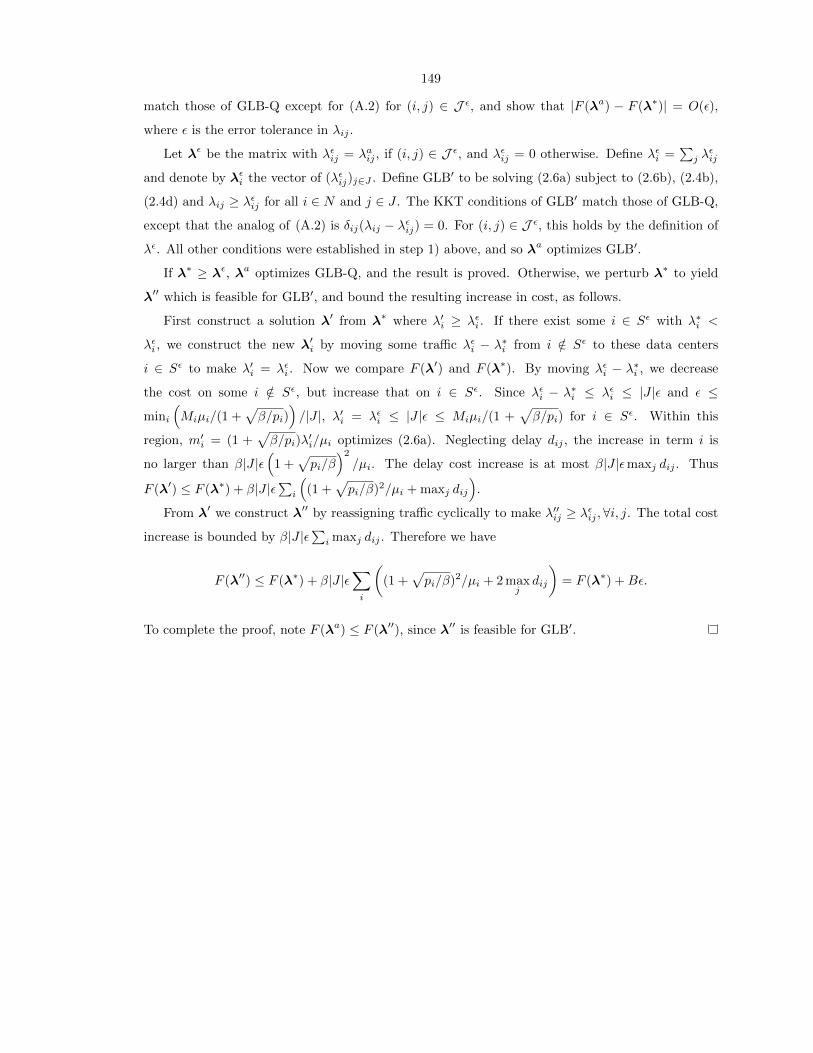
149

match those of GLB-Q except for (A.2) for (i, j) ∈ J ε, and show that |F (λa) − F (λ∗)| = O(ε),

where ε is the error tolerance in λij .

Let λε be the matrix with λεij = λaij , if (i, j) ∈ J ε, and λεij = 0 otherwise. Define λεi =∑j λ

εij

and denote by λεi the vector of (λεij)j∈J . Define GLB′ to be solving (2.6a) subject to (2.6b), (2.4b),

(2.4d) and λij ≥ λεij for all i ∈ N and j ∈ J . The KKT conditions of GLB′ match those of GLB-Q,

except that the analog of (A.2) is δij(λij − λεij) = 0. For (i, j) ∈ J ε, this holds by the definition of

λε. All other conditions were established in step 1) above, and so λa optimizes GLB′.

If λ∗ ≥ λε, λa optimizes GLB-Q, and the result is proved. Otherwise, we perturb λ∗ to yield

λ′′ which is feasible for GLB′, and bound the resulting increase in cost, as follows.

First construct a solution λ′ from λ∗ where λ′i ≥ λεi . If there exist some i ∈ Sε with λ∗i <

λεi , we construct the new λ′i by moving some traffic λεi − λ∗i from i /∈ Sε to these data centers

i ∈ Sε to make λ′i = λεi . Now we compare F (λ′) and F (λ∗). By moving λεi − λ∗i , we decrease

the cost on some i /∈ Sε, but increase that on i ∈ Sε. Since λεi − λ∗i ≤ λεi ≤ |J |ε and ε ≤

mini

(Miµi/(1 +

√β/pi)

)/|J |, λ′i = λεi ≤ |J |ε ≤ Miµi/(1 +

√β/pi) for i ∈ Sε. Within this

region, m′i = (1 +√β/pi)λ

′i/µi optimizes (2.6a). Neglecting delay dij , the increase in term i is

no larger than β|J |ε(

1 +√pi/β

)2

/µi. The delay cost increase is at most β|J |εmaxj dij . Thus

F (λ′) ≤ F (λ∗) + β|J |ε∑i

((1 +

√pi/β)2/µi + maxj dij

).

From λ′ we construct λ′′ by reassigning traffic cyclically to make λ′′ij ≥ λεij ,∀i, j. The total cost

increase is bounded by β|J |ε∑i maxj dij . Therefore we have

F (λ′′) ≤ F (λ∗) + β|J |ε∑i

((1 +

√pi/β)2/µi + 2 max

jdij

)= F (λ∗) +Bε.

To complete the proof, note F (λa) ≤ F (λ′′), since λ′′ is feasible for GLB′.

150

Appendix B


B.1 Proof of Theorem 8

By the definition of convexity, we need to prove ∀da, db ∈ [0, D],∀θ ∈ [0, 1], c(θda + (1 − θ)db) ≤

θc(da) + (1 − θ)c(db). Denote by da1 and da2 the optimal cooling capacities of chiller cooling and

outside air cooling for the total IT heat load da, respectively. This optimal solution exists because

the feasible set is compact. Then we have da1 +da2 = da and c(da) = fc(da1)+fo(d

a2) by the optimality

of da1 and da2 . Similarly, we denote the optimal solution for db by db1 and db2, and we know db1 +db2 = db

and c(db) = fc(db1) + fo(d

b2). Then we have

c(θda + (1− θ)db)

= c(θda1 + θda2 + (1− θ)db1 + (1− θ)db2)

≤ fc(θda1 + (1− θ)db1) + fo(θda2 + (1− θ)db2)

≤ θfc(da1) + (1− θ)fc(db1) + θfo(da2) + (1− θ)fo(db2)

= θc(da) + (1− θ)c(db).

Here the first inequality is from the fact that c(d) is the optimal allocation of cooling capacities and

the expression in the third line is just one possible allocation, and the feasible set is convex. The

second inequality is from the convexity of both fc(d) and fo(d).


We prove this by contradiction. Assume there exist two optimal solutions (d1, e1) and (d2, e2)

with different (d(t) + c(d(t))− r(t)− e(t))+for time t. Then the linear combination (dc, ec) :=

(θd1 + (1− θ)d2, θe1 + (1− θ)e2) , 0 < θ < 1 is also an optimal solution. Then, the energy cost at

151

time t of (dc, ec) is:

p(t)(θd1(t) + (1− θ)d2(t) + c(θd1(t) + (1− θ)d2(t))

− r(t)− θe1(t)− (1− θ)e2(t))+

< p(t)(θd1(t) + (1− θ)d2(t) + θc(d1(t)) + (1− θ)c(d2(t))

− r(t)− θe1(t)− (1− θ)e2(t))+

≤ p(t)(θ (d1(t) + c(d1(t))− r(t)− e1(t))+

+ (1− θ) (d2(t) + c(d2(t))− r(t)− e2(t))+)

= θp(t) (d1(t) + c(d1(t))− r(t)− e1(t))+

+ (1− θ)p(t) (d2(t) + c(d2(t))− r(t)− e2(t))+

Here the first inequality is from the strictly convexity of c(d) and p(t) > 0, the second inequality is

from the convexity of the (·)+ function and p(t) > 0.

All the other parts of the objective function do not increase because of convexity, so the value

of the objective function of (dc, ec) is strictly lower than that of (d1, e1), which contradicts the fact

that (d1, e1) is an optimal solution.


Begin by defining D := ∂(d(t) + c(d(t))− e(t)− r(t))+/∂d(t).

Next, notice that (d(t) + c(d(t)) − e(t) − r(t))+ can be divided into three parts: (i) It is 0 for

d ≤ ds1, where ds1 is the switching point of (d(t) + c(d(t))− e(t)− r(t))+ from 0 to strictly positive.

(ii) It is strictly positive and strictly convex for ds1 < d < ds2, where ds2 is the switching point

between using outside air and using the chiller. (iii) It is constant for d ≥ ds2 due to the linear

chiller power function.

If there exist two optimal solutions (d1, e1) and (d2, e2) with different D at time t, then there

are seven cases based on which of the above sections d1 and d2 are in. By combining the redundant

cases, we need only consider the following four cases:

(a) d1(t) ≤ ds1, ds1 < d2(t) < ds2

(b) d1(t) ≤ ds1, d2(t) ≥ ds2

(c) ds1 < d1(t) < ds2, ds1 < d2(t) < ds2, but d1(t) 6= d2(t)

(d) ds1 < d1(t) < ds2, d2(t) ≥ ds2

For each case, it is straightforward to show that taking a linear combination of the two solutions

decreases the objective, which contradicts the fact that (d1, e1) is an optimal solution. The proof is

similar to the proof of Theorem 8.

152


For each optimal solution S, consider an undirected bipartite graph G with a vertex representing each

class of batch jobs and each time slot and with an edge connecting i and j when 0 < bj(t) < MPj .

We will show that at least one of these graphs is acyclic. The theorem then follows since an

acyclic graph with K nodes has at most K − 1 edges. To prove that there exists an optimal

solution whose graph is acyclic, we will inductively reschedule batch jobs in a way that removes

cycles while preserving optimality. Suppose there exists an optimal solution S whose graph G

contains a cycle. Let C be a minimal cycle, i.e., no strict subset of C is a cycle. Let (t∗, j∗) =

arg min(t,j)∈C (minbj(t),MPj − bj(t)).

Then let C be directed so that (j∗, t∗) ∈ C if (t∗, j∗) = arg min(t,j)∈C bj(t) and (t∗, j∗) ∈ C

if (t∗, j∗) = arg min(t,j)∈CMPj − bj(t). Form a new solution S(ξ) from S by adding ξ to bj(t) if

(t, j) ∈ C, and subtracting ξ from bj(t) if (j, t) ∈ C. Note that this does not change the∑j bj(t)

and∑t bj(t), therefore it does not change the cost.

If (t∗, j∗) = arg min(t,j)∈C bj(t), then S(bj∗(t∗)) has bj∗(t

∗) = 0. If (t∗, j∗) = arg min(t,j)∈CMPj−

bj(t), then S(MPj − bj∗(t∗)) has bj∗(t∗) = MPj . In either case, the new solution has at least one

fewer cycle, since it has broken C. Further, by construction, it is still optimal.

153

Appendix C


In this appendix we include proofs for bounds on the competitive ratio of our both algorithms in

Section 4.3. Because the proof of Theorem 12 uses simplified versions of many parts of the proof of

Theorem 13, we start with the proof of Theorem 13 and then describe how to specialize the approach

to Theorem 12.

C.1 Proofs of Theorem 12 and 13

To prove Theorem 13, we start with some notation and simple observations. First, in this context,

the offline optimal is defined as follows: (b∗,g∗) ∈ argminb,gf∗(e,g), where f∗(e,g) ≡ Σtp(t)e(t)+

ppmaxte(t) + pcpe(tcp) + pgΣtg(t). Here b stands for the workload management, and g denotes the

local backup generator usage, e(t) = (d(t) − r(t) − g(t))+ is the grid power usage, we assume the

offline optimal have perfect knowledge of d(t), r(t), and when coincidental peak occurs.

In contrast, the plan derived from Algorithm 5, denoted by (ew1 ,gw1 ), minimizes

fw(e,g) ≡ Σtp(t)e(t) +(pp + W (pg −mintp(t))

)maxte(t) + pgΣtg(t)

using prediction of workload d(t) and prediction of renewable generation r(t) without any knowledge

of coincidental peak (CP) or warnings except W . Here e(t) = (d(t) − r(t) − g(t))+. In addition,

Algorithm 5 uses minimal local generation to remove harmful prediction error when (4.4) occurs,

i.e., gwε (t) = max0,minew(t), εddw(t)−εr r(t). Also, Algorithm 5 uses local generation whenever

warnings are received, i.e., gw2 (t) = It∈Wew1 (t),∀t, where It∈W is the indicator function, which

equals to 1 if t is a time when warning is received and 0 otherwise and ew1 (t) = (dw1 (t) − r(t) −

gw1 (t) − gwε (t))+. Therefore the real grid power usage at time t is ew(t) ≤ ew1 (t) − gw2 (t), and local

power generation is gw(t) = gw1 (t) + gwε (t) + gw2 (t),∀t. Note here (ew1 ,gw1 ) is the day-ahead plan,

while (ew,gw) is the real grid power consumption and local generation after using local generation

to compensate for underestimation and during warning periods.

154

Proof of Theorem 13. Note that f∗ and fw are optimizations using different data (f∗ uses perfect

knowledge of d(t) and r(t), while fw uses prediction d(t) and r(t)), to bridge this gap, we first

observe the following:

f∗(e∗,g∗) ≥ f∗(e∗,g∗ + g∗ε)− pgΣtg∗ε (t) (C.1)

where e∗ is the optimizer of f∗ using prediction d(t) and r(t), and g∗ε is defined in a similar way to

gwε , g∗ε (t) = max0,mine∗(t), εdd(t)−εr r(t) which removes all the harmful prediction errors. The

right hand side of the inequality is essentially evaluating the same objective using prediction, but

is given g∗ε of local power for free. As g∗ε removes all harmful effects of prediction, using prediction

will not increase the objective.

The key step is to bound Eξd,ξr [fw(ew1 ,g

w1 )] in terms of Eξd,ξr [f

∗(e∗,g∗ + g∗ε)]

Eξd,ξr [f∗(e∗,g∗ + g∗ε)]

= Eξd,ξr [fw(e∗,g∗ + g∗ε))]− W (pg −mintp(t))Eξd,ξr [maxte

∗(t)] + pcpEξd,ξr [e∗(tcp)]

≥ Eξd,ξr [fw(e∗,g∗ + g∗ε))]− W (pg −mintp(t))Eξd,ξr [maxte

∗(t)]

≥ Eξd,ξr [fw(ew1 ,g

w1 )]− W (pg −mintp(t))Eξd,ξr [maxte

∗(t)]

≥ Eξd,ξr [fw(ew1 ,g

w1 + gwε )]− pgΣtEξd,ξr [g

wε (t)]− W (pg −mintp(t))Eξd,ξr [maxte

∗(t)]

≥ Eξd,ξr [f∗(ew,gw)]− pgΣtEξd,ξr [g

wε (t)]− W (pg −mintp(t))Eξd,ξr [maxte

∗(t)] (C.2)

Here the first inequality holds because pcpEξd,ξr [e∗(tcp)] ≥ 0. The second inequality is from the

optimality of (ew1 ,gw1 ) in minimizing fw(e,g). However, the last inequality is more involved.

We show the last step of (C.2) by first writing out the day-ahead plan ew1 (t) =(dw1 (t)− r(t)− gw1 (t)

)+

,

and the actual power demand ew(t) = (dw1 (t)− r(t)− gw1 (t)− gwε (t)− gw2 (t))+

. Furthermore, denote

ew2 (t) as the electricity demand of Algorithm 5 without using local generation to respond to CP warn-

ing. Then ew(t) = ew2 (t)− gw2 (t), and gw2 (t) = ew2 (t)It∈W, so we have

ew2 (t) = (dw1 − r(t)− gw1 (t)− gwε (t))+ ≤

(dw1 (t)− r(t)− gw1 (t)

)+

= ew1 (t)

155

Hence ew(t) = ew2 (t)− gw2 (t) ≤ ew1 (t)− gw2 (t). Next, we bound f∗(ew,gw) as follows.

f∗(ew,gw) = f∗(ew,gw1 + gwε + gw2 )

= Σtp(t)ew(t) + ppmaxte

w(t) + pcpew(tcp) + pgΣtg

w(t)

= Σt/∈W p(t)ew2 (t) + ppmaxt/∈W e

w2 (t) + pg (Σt(g

w1 (t) + gwε (t)) + Σt∈W e

w2 (t))

≤ Σtp(t)ew1 (t) + ppmaxte

w1 (t) + pgΣt(g

w1 (t) + gwε (t)) + Σt∈W (pg − p(t))ew1 (t)

≤ Σtp(t)ew1 (t) + ppmaxte

w1 (t) + pgΣt(g

w1 (t) + gwε (t)) + W (pg −mintp(t))maxte

w1 (t)

= fw(ew1 ,gw1 + gwε ) (C.3)

The second equality is because gw2 (t) = It∈Wew2 (t),∀t. The first inequality is from maxt/∈W e

w2 (t) ≤

maxtew2 (t) and ew2 (t) ≤ ew1 (t). The second inequality holds because Σt∈W (pg − p(t))ew1 (t) ≤

Σt∈W (pg −mintp(t))ew1 (t)

= (pg −mintp(t)) Σt∈W ew1 (t) ≤ (pg −mintp(t)) Σt∈Wmaxte

w1 (t) ≤ W (pg −mintp(t))maxte

w1 (t).

Finally, we can combine (C.1) and (C.2) to obtain

Eξd,ξr [f∗(e∗,g∗)]

≥ Eξd,ξr [f∗(e∗,g∗ + g∗ε)]− pgΣtEξd,ξr [g

∗ε (t)]

≥ Eξd,ξrf∗(ew,gw)− pgΣtEξd,ξr [g

wε (t) + g∗ε (t)]− W (pg −mintp(t))Eξd,ξr [maxte

∗(t)]

≥ Eξd,ξr [f∗(ew,gw)]− pgσΣt

(dw(t) + d∗(t)

2+ r(t)

)− W (pg −mintp(t))Eξd,ξrmaxte

∗(t),

(C.4)

where (C.4) derives from the following

Eξd,ξr [gwε (t) + g∗ε (t)]

= Eξd,ξr [max0,minew(t), εddw(t)− εr r(t)+ max0,mine∗(t), εdd∗(t)− εr r(t)]

≤ Eξd,ξr [(εddw(t)− εr r(t))+] + Eξd,ξr [(εdd

∗(t)− εr r(t))+]

= E[εw(t)+] + E[ε∗(t)+](

let εw(t) = εddw(t)− εr r(t), ε∗(t) = εdd

∗(t)− εr r(t))

≤ 1

2σεw(t) +

1

2σε∗(t)

=1

2

(√dw(t)2σ2

d + r(t)2σ2r +

√d∗(t)2σ2

d + r(t)2σ2r

)≤ 1

2

((dw(t) + r(t)) max(σd, σr) + (d∗(t) + r(t)) max(σd, σr)

)=

(dw(t) + d∗(t)

2+ r(t)

)σ (C.5)

The second last equality holds because εd and εr are independent, and the last inequality holds

156

because d(t) and r(t) are nonnegative.

The key is the second inequality, as the cases for εw(t) and ε∗(t) are the same, we just need to

show this inequality holds for any ε(t) has zero mean and fixed variance σ2ε(t). Note that ε(t) =

ε(t)+ − ε(t)−, hence E[ε(t)] = 0⇒ E[ε(t)+] = E[ε(t)−]. It follows that

σ2ε(t) = E[ε(t)2]

= E[(ε(t)+)2] + E[(ε(t)−)2]− 2E[ε(t)+ε(t)−]

= E[(ε(t)+)2] + E[(ε(t)−)2]

≥ E[ε(t)+]2

P(ε(t) ≥ 0)+

E[ε(t)−]2

P(ε(t) < 0)

= E[ε(t)+]2(

1

P(ε(t) ≥ 0)+

1

1− P(ε(t) ≥ 0)

)= E[ε(t)+]2

(1

(P(ε(t) ≥ 0))(1− P(ε(t) ≤ 0))

)≥ 4E[ε(t)+]2

Rearranging, we have E[ε(t)+] ≤ 12σε(t). The last inequality attains equality when P(ε(t)+ ≥ 0) =

P(ε(t)− < 0) = 1/2. The third equality follows because ε(t)+ and ε(t)− cannot be simultaneously

non-zero. The first inequality follows because

E[(ε(t)+)2]P(ε(t) ≥ 0)

=

ˆ ∞0

x2dFε(t)(x)

ˆ ∞0

1dFε(t)(x)

≥(ˆ ∞

0

x · 1dFε(t)(x)

)2

= E[ε(t)+]2

⇒ E[(ε(t)+)2] ≥ E[ε(t)+]2

P(ε(t) ≥ 0)

The first inequality follows from Cauchy-Schwarz inequality, and the inequality attains equality when

the distribution of ε(t)+ is a point mass. By similar argument we can show that E[ε(t)−]2 ≥ E[ε(t)−]2

P(ε(t)<0) ,

and equality is attained when the distribution of ε(t)− is a point mass.

Using the observation above and the previous observation that P(ε(t)+ ≥ 0) = P(ε(t)− < 0) =

1/2, we can see that E[ε(t)+] = 12σε(t) when the distribution of ε(t) is two equal point masses located

at σε(t) and σε(t) respectively.

Finally, combining the above, we can compute the competitive ratio as follows

157

12

0−σε(t) σε(t)x

P(ε(t) = x)

Figure C.1: Illustration of pdf of ε(t) that attains E[ε(t)+] = 12σε(t) for E[ε(t)] = 0 and V [ε(t)] =

σ2ε(t).

Eξd,ξr [f∗(ew,gw)]


≤ 1 +W (pg −mintp(t))Eξd,ξr [maxte

∗(t)] + pgσΣt

(dw(t)+d∗(t)

2 + r(t)))

Σtp(t)Eξd,ξr [e∗(t)] + ppEξd,ξr [maxte∗(t)] + pcpEξd,ξr [e

∗(tcp)] + pgΣtg∗(t)

≤ 1 +W (pg −mintp(t))

Σtp(t)Eξd,ξr [e∗(t)]/Eξd,ξr [maxte∗(t)] + pp

+Bσ,

(B =

pgΣt(dw(t)+d∗(t)

2 + r(t))


)(C.6)


mintp(t)ΣtEξd,ξr [e∗(t)]/Eξd,ξr [maxte∗(t)] + pp

+Bσ

= 1 +W (pg −mintp(t))

Tmintp(t)/PMR∗ + pp+Bσ


pp+Bσ

It remains to show that no online algorithm can have competitive ratio smaller than (1 +

W (pg−mintp(t))pp

) even with perfect information of workload and renewable generation. To prove

this, we use the instance summarized in Figure C.2.

In this instance, PUE is the same across all time slots and small. There is no local renewable

supply or interactive workload. The total flexible workload demand is D. The (discrete) time

horizon is [1,T], where twi, i = 1, ...,W are the time slots with warnings (three warnings are shown

in the figure) and the total number of warnings is W with bound W ≥ W known to the online

algorithm. The final coincident peak hour is tcp and it is among the warnings (tw3 in the figure).

The usage-based electricity price p(t) = p,∀t and is much smaller than pp and pcp. Also, in this

instance,ppT−1 ≤ pg (using local generation is more expensive than demand shifting and paying

(slightly) increased peak demand charging) and pg ≤ pcp, which are common in practice.

In this setting, the offline optimal solution plans according to the green curve: it does not use

the coincident peak time slot but spreads the demand evenly across the other T − 1 time slots. The

cost of the offline optimal solution is therefore f∗(e∗,g∗) = pD + ppDT−1 .

158

T time

demand

D/(T-1)

tw3 (tcp)

OPT

ALG D/T

tw1 tw2

Local generation

Figure C.2: Instance for lower bounding the competitive ratio for setting with local generation.

In contrast, any online algorithm can at best plan according to the red curve: spreading the

workload evenly among all T time slots and using local generation when warnings are received. To

see this, note that there is no benefit to spreading the workload unevenly since that increases local

generation usage for the worst-case instance and possibly the peak charging, while not saving any

usage based cost. The cost of the best online non-adaptive solution is therefore f∗(eALG,gALG) =

pD + ppDT +W (pg − p) DT . The best competitive ratio is therefore:

f∗(eALG,gALG)

f∗(e∗,g∗)=pD + pp

DT

+W (pg − p) DTpD + pp

DT−1

= 1 +−pp D

T (T−1)+W (pg − p) DT

pD + ppDT−1

= 1 +W (pg − p)− pp

T−1

pT + ppTT−1

As T → ∞, taking the usage cost pT as the same or smaller order of magnitude as the peak cost

pp, this becomes

1 +W (pg − p)pT + pp

The above matches the bound in equation (C.6) when W = W , which completes the proof.

Proof Sketch of Theorem 12. The proof of Theorem 12 is similar in structure to that of Theorem 13,

only simpler. Thus, we outline only the main steps and highlight the similarities with the proof of

Theorem 13. In particular, the following provides the major steps needed to bridge the expected cost

of Algorithm 4 and the cost of the offline algorithm with exact IT demand and renewable generation

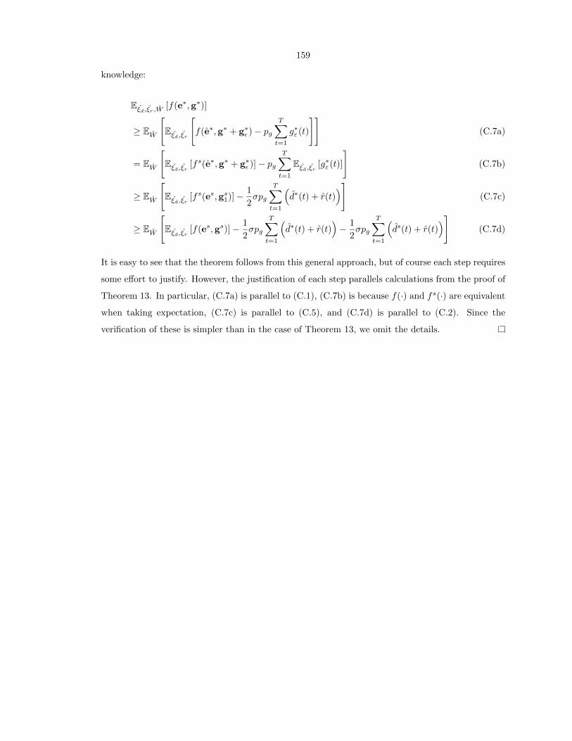
159

knowledge:

Eξd,ξr,W [f(e∗,g∗)]

≥ EW

[Eξd,ξr

[f(e∗,g∗ + g∗ε )− pg

T∑t=1

g∗ε (t)

]](C.7a)

= EW

[Eξd,ξr [fs(e∗,g∗ + g∗ε )]− pg

T∑t=1

Eξd,ξr [g∗ε (t)]

](C.7b)

≥ EW

[Eξd,ξr [fs(es,gs1)]− 1

2σpg

T∑t=1

(d∗(t) + r(t)

)](C.7c)

≥ EW

[Eξd,ξr [f(es,gs)]− 1

2σpg

T∑t=1

(d∗(t) + r(t)

)− 1

2σpg

T∑t=1

(ds(t) + r(t)

)](C.7d)

It is easy to see that the theorem follows from this general approach, but of course each step requires

some effort to justify. However, the justification of each step parallels calculations from the proof of

Theorem 13. In particular, (C.7a) is parallel to (C.1), (C.7b) is because f(·) and fs(·) are equivalent

when taking expectation, (C.7c) is parallel to (C.5), and (C.7d) is parallel to (C.2). Since the

verification of these is simpler than in the case of Theorem 13, we omit the details.

160

Appendix D

Appendix: Proofs of Chapter 5

D.1 Proof of Theorem 14

To begin, we compute as follows:

g′(p) = −h′(D −

∑i

si(p)

)∑i

s′i(p) +∑i

c′i(si(p))s′i(p)

=∑i

s′i(p)

(c′i(si(p))− h′

(D −

∑i

si(p)

))

=

(p− h′

(D −

∑i

si(p)

)) ∑i

s′i(p),

where the last equality follows from c′i(si(p)) = p for all i. Our assumptions imply that s′i(p) =

(c′′i (si(p)))−1

> 0, and hence g′(p) = 0 if and only if

v(p) := p− h′(D −

∑i

si(p)

)= 0.

Now, v(0) = −h′(D) ≤ 0, v(p) = p > 0, and v(p) is strictly increasing. Hence a unique 0 ≤ p∗ < p

satisfies v(p∗) = 0. Moreover g′(p) < 0 for p < p∗ and g′(p) > 0 for p > p∗ implying that p∗ is the

unique minimizer of g(p).

161


We first evaluate E [G(p∗)]. From Theorem 14

p∗ = h′

(D −

∑i

si(p∗)

)

= q

(D − p∗

∑i

Xi

)= qD − qXp∗.

Hence

p∗ =q

1 + qXD, (D.1)

which is a random (optimal) price.

Next, from (5.10) and (D.1) we have

E [G(p∗)] =qD2

2E[

1

1 + qX

], (D.2)

where the expectation is taken over X.

To evaluate (5.7) we have, using (5.10),

E [G(p)] = minp≥0

E[q

2(D −Xp)2 +

1

2Xp2

]= min

p≥0

1

2

((qE[X2]

+ E [X])p2 − 2qDE [X] p+ qD2

).

Consequently, the unique minimizer p and the optimal value of (5.7) are

p =qE [X]

qE [X2] + E [X]D, (D.3)

E [G(p)] =qD2

2

E [X] + qV [X]

E [X] + qE [X2]. (D.4)

We can now quantify the competitive ratio using (D.2) and (5.18). Jensen’s inequality implies

E [G(p∗)] ≥ qD2

21

1+qE[X] . Thus,

E [G(p)]

E [G(p∗)]≤ E [X] + qV [X]

E [X] + qE [X2](1 + qE [X])

= 1 +q2E [X]

E [X] + qE [X2]V [X] .

162

Rewriting the above in terms of the square coefficient of variation C2[X] gives:

E [G(p)]

E [G(p∗)]≤ 1 +

(qE[X])2C2[X]

1 + (qE[X])(C2[X] + 1).

Finally, to compare p in (D.3) with p∗ in (D.1) we can rewrite p as

p =qD

1 + qE[X](C2[X] + 1).

Hence

E [p∗] = E[

qD

1 + qX

]≥ qD

1 + qE [X]≥ qD

1 + qE[X](C2[X] + 1)= p,

where the first inequality follows from the Jensen’s inequality and the second inequality follows from

C2[X] ≥ 0. Both of these are equalities if and only if X has zero variance.


To show tightness we focus on the only inequality used in the proof of Theorem 15, which is

E [G(p∗)] ≥ qD2

2(1 + E [X]).

We need to show that, for any ε > 0, there exists a probability distribution f(X) with mean E [X]

and variance V [X] such that

E [G(p∗)] ≤ qD2

2(1 + E [X])+ ε.

We define such a probability distribution as follows. For any 0 < x < 1, let d1 := E [X] −√V [X] (1− x)/x and d2 := E [X]+

√V [X]x/(1− x). Then define the following probability density

function:

fx(X) = xδ(E [X]− d1) + (1− x)δ(E [X]− d2), (D.5)

where

δ(a) :=

∞ if a = 0

0 otherwise

163

and´δ(a)da = 1.

Note that for any 0 < x < 1, the probability distribution defined in (D.5) has mean E [X] and

variance V [X] and

limx→1

E [G(p∗)] =qD2

2(1 + E [X]).

Thus, the bound is tight.

D.4 Proof of Corollary 1

Given E [X(n)] = nα and V [X(n)] = nσ2, we have C2[X] = σ2

nα2 . Thus, we can compute as follows.

E [G(p)]

E [G(p∗)]≤ 1 +

(qE[X])2C2[X]

1 + (qE[X])(C2[X] + 1)

= 1 +q2n2α2 σ2

nα2

1 + qnα(σ2

nα2 + 1)

= 1 +q2α2

qα3

σ2 +(α2

σ2 + qα)/n

→ 1 +qσ2

αas n→∞.


To prove that the competitive ratio of prediction-based pricing does not become larger when there

are constraints on the space of prices, i.e., p ∈ [p, p], we consider two cases. The cases are diagramed

in Figure D.1.

Case 1 Case 2

Figure D.1: Diagram of cases for proof of Theorem 17.

Case 1: The price p∗ picked by the clairvoyant algorithm is within the feasible set [p, p], i.e.,

164

p∗ ∈ [p, p]. We have p∗R = p∗ and therefore g(p∗R) = g(p∗). If the price picked by our algorithm

p ∈ [p, p], then we have pR = p and therefore g(pR) = g(p). Hence g(p)g(p∗) = g(pR)

g(p∗R) .

Otherwise p /∈ [p, p]. We have pR = p if p < p and pR = p if p > p. In either case g(pR) ≤ g(p),

and therefore g(p)g(p∗) ≥

g(pR)g(p∗R) .

Case 2: The price p∗ picked by th clairvoyant algorithm is outside the feasible set [p, p]. Without

loss of generality, we assume p∗ < p, as shown in the figure. We have p∗R = p and g(p∗R) ≥ g(p∗). If

the price picked by our algorithm p ∈ [p, p], then we have pR = p and therefore g(pR) = g(p). Hence

g(p)g(p∗) ≥

g(pR)g(p∗R) .

Otherwise p /∈ [p, p]. We have pR = p if p < p and pR = p if p > p. In the first case we have

pR = p∗R = p and therefore g(pR) = g(p∗R), hence g(p)g(p∗) ≥

g(pR)g(p∗R) = 1. In the second case we have

g(pR) ≤ g(p), and therefore g(p)g(p∗) ≥

g(pR)g(p∗R) .

Education

Sustainable it and it for sustainability