The Linkages of Financial Liberalization and Currency Stability: What do we learn from Pre and Post Asian Financial Crisis?

a

IBIMA PublishingJournal of Economics Studies and Research.http://www.ibimapublishing.com/journals/JESR/jesr.htmlVol. 2013 (2013), Article ID 235134, 9 pagesDOI: 10.5171/2013.235134

The Linkages of Financial Liberalization andCurrency Stability: What do we learn from

Pre and Post Asian Financial Crisis?

Wahyu Ario Pratomo1, Suwandi2 and Ari Warokka1

1Economic Development Department, Faculty of Economics – North Sumatera University, Indonesia

2Faculty of Economics – Cenderawasih University, Indonesia

Abstract

The tendency of repeating history has made any financial crisis a valuable source to be exploredand studied. It will make people be more prepared and ready to anticipate. This paperexamined the nature of linkages between exchange rate and macroeconomic fundamentals over1997-2004. It investigated the evidence on both the short- and long-run effects of exchange ratedeterminant factors using co-integration theory. It also explored the stability of rupiah duringthe pre and post economic crisis, seeking whether the Indonesian currency was overshooting ornot. To test the stability of rupiah after monetary and fiscal liberalization, we employed theChow test. The results revealed that the rupiah was overshooting during the crisis' period andthere was a structural change of rupiah after 1998. Due to the significant effects of interest rateand exchange rate on the currency stability, it is important to the Indonesia’s monetaryinstitution to be aware of these two variables, especially in stabilizing the economicperformance after the financial liberalization. The elasticity obtained for relative money supply(m) is greater than unity indicating that this result consistent with overshooting hypothesis.

Keywords: Financial liberation, currency stability, cointegration theory, economic crisis.

Introduction

Indonesia's economic reforms began in themid 1980s, when government made amonetary and fiscal deregulation in 1983.Over the next decade, reforms wereexpected at opening the real economy bypromoting direct investment flows andliberalizing the financial sector, increasingcompetition, and promoting growth.

The government aimed to support thesereforms with improved macroeconomicmanagement, including through an attemptto maintain a competitive and stableexchange rate. The exchange rate policywas first changed in December 1978 from apegged regime to a managed floatingexchange rate system. The rupiah was

linked to a basket of currencies consistingof Indonesia’s main trading partners.

The crude petroleum and natural gasdominated the Indonesia’s export tradeuntil the mid 1980s. Hence, the oil pricelargely influenced and determined thegovernment‘s earnings. The collapse of oilprice in 1986 led to a devaluation, andgovernment was pushed to boost non-oil/gas exports.

After the two major devaluations in 1983and 1986, Bank Indonesia strived tointervene against the foreign exchangemarket in order to stabilize the exchangerate, country’s foreign exchange reservesand monetary system.

Copyright © 2013 Wahyu Ario Pratomo, Suwandi and Ari Warokka. This is an open access article distributed under the Creative Commons Attribution License unported 3.0, which permitsunrestricted use, distribution, and reproduction in any medium, provided that original work is properlycited. Contact author: Wahyu Ario Pratomo E-mail: [email protected]

Journal of Economics Studies and Research

When the financial crises occurred in 1997,rupiah depreciated and continued to slideand exceeded the upper limit of theintervention band. Bank Indonesia decidedto float the rupiah on August 14, 1997.Indonesia was the worst sufferer in theAsian crisis. The nominal exchange ratejumped from Rp2400 per US dollar toalmost Rp17000 per US dollar in mid 1998.

This paper attempts to analyze and test themonetary approach and the overshootinghypothesis in Indonesia. It emphasizes theeffect of financial liberalization to theexchange rate of Indonesia in the period ofbefore and after the economic crisis. Themodel of exchange rate determination isexpressed as a function of the relativemoney supply, relative income level, thenominal interest differential and theexpected long-run inflation differential. Weuse the ordinary least square (OLS) methodin the analysis and applying the Chow testin order to explore the stability of rupiahbefore and after the economic crisis.

Literature Review

As the fixed exchange rate system hadterminated, many of the literatures beganto explain the exchange rate changes.These literatures are laid on monetary orasset view. The older theories of exchangerate are focused more on trade of accountof the balance of payments, while newtheories; that are called “asset view,"focused on a stock approach.

Frankel (1979) suggests that there are twovery different approaches in new theories.The first approach might be called theChicago theory. It assumes that prices areperfectly flexible. If there is a change innominal interest rate, it will reflect changesin the expected inflation rate. When thedomestic interest rate rises relative to theforeign interest rate, there will be adecrease in home currency throughinflation and depreciation. So there will bea positive relationship between theexchange rate and the nominal interest ratedifferential.

The second approach might be called theKeynesian theory. It assumes prices are

sticky, at least in the short run. If there is achange in the nominal interest rate, it willreflect changes in the tightness ofmonetary policy. When the domesticinterest rate rises relative to the foreignrate, it will attract a capital inflow, whichcauses the home currency to appreciate. Sothere will be a negative relationshipbetween exchange rate and the nominalinterest differential.

The monetary approach to exchange ratedetermination focuses on the moneymarket. The interaction between moneydemand and money supply results in anequilibrium exchange rate. Thus, theexchange rate is seen as the equilibriumprice between two stocks of money.

In the monetary model, there are someassumptions applied. Firstly, the moneysupply is assumed to be stable andexogenous. Secondly, assets are perfectlysubstitutable; therefore, UIP (UncoveredInterest Parity) holds continuously.Thirdly, the demand for money is a stablefunction of fundamental variables such asincome and interest rate. Fourthly, incomeis assumed to be at its full-employmentlevel. Finally, PPP is assumed to holdcontinuously.

The exchange rate of a monetary model isdetermined by relative money demandsand money supplies. If domestic incomeincreases fairly to foreign income, then thedemand of money for domestic willincrease relatively to the supply.Consequently, this causes the exchangerate appreciates. By contrast, an increase inthe domestic money supply causes toaugment in the exchange rate. The excesssupply of money results in depreciating theexchange rate respectively. Similarly, ifexpected domestic inflation rises about theexpected in the foreign country, then thedemand for money falls and the exchangerate will depreciate.

Dornbusch (1976) introduced his sticky-price monetary model, which contained anovershooting hypothesis. The main featureof his model is that since prices are stickyin the short-run, an increase in the moneysupply will result in lower interest rate and


thus capital outflow, will cause currencydepreciation. In the short run, the currencywill overshoot itself. However, over time,commodity prices will rise and result in adecrease in real money supply and higherinterest rate. In the end, the currency willappreciate.

The empirical researches about theexchange rate determinants are varied. Theworks of Frankel (1979), Driskill (1981),and Papel (1998) provide the overshootingmodel, while Backus (1981) and Flood andTaylor (1996) do not. Hairault et al. (2004)finds that an expansionary monetary policyimplies an increase in interest rate and adepreciation of the exchange rate.

Obstfeld and Rogoff (2000) have recentlyunderlined the difficulty in estimating theexchange rate volatility. Any models areunderlying fundamentals such as interestrates, outputs and money supplies but nomodel seems to be very good at explainingexchange rates even ex-post.

Model

The theory of monetary approach beginswith two fundamental assumptions. Thefirst is the interest rate parity. The marketis efficient which bonds of differentcountries are substitutable.

d= r – r* (1)

Where r is defined as the log of one plus thedomestic rate of interest and r* is definedas the log of one plus the foreign rate ofinterest. If d is considered to be theforward discount, defined as the log of theforward rate minus the log of the currentspot rate, subsequently equation (1) is astatement of covered (or closed) interestparity. However, d will be defined as theexpected rate of depreciation; then

equation (1) represents the strongercondition of uncovered interest rate parity.

The second is that the expected rate ofdepreciation is a function of the gapbetween the current spot and anequilibrium rate, and of the expected long-run inflation differential between thedomestic and foreign countries:

d = - (e - e ) + - * (2)

Where e is the log of the spot rate andand * are the expected inflation home andforeign country. The log of the equilibriumexchange rate e is defined to increase atthe rate of - *. Equation (2) says that inthe short run the exchange rate is expectedto return to its equilibrium value at a ratewhich is proportional to the current gap,

and in the long run when e = e , it isexpected to change at the long-run rate -

*. The rational value of will be seen to beclosely to the speed of adjustment in thegood market.

Combining equation (1) and (2) gives:

e e1

[(r ) (r * *)] (3)

The equation in the bracket shows the realinterest rate differential. When a tightmonetary policy in one country causes thenominal interest differential to rise aboveits long-run level, an incipient capitalinflow causes the value of the currency to

rise proportionally above its equilibriumlevel.

Assuming that in the long run, purchasingpower parity holds:

e p p * (4)


Where p and p* are defined as the logs ofthe equilibrium price level at home andforeign country.

Assume that the function of money demandequation:

m = p + y - r (5)

Where m, p and y are defined as the logs ofthe domestic money demand, price leveland output. Assume also money demandequals to the money supply. A similar

equation holds abroad, and the differentbetween the two equations for home andforeign are:

m – m* = p – p* + (y-y*) - (r-r*) (6)

Considering that in the long run,e e , r r*, * , we get

e p p * (7)

e m m * (y y*) (r r*) ( *) (8)

This equation illustrates the exchange rateof monetary theory is determined by therelative supply of and demand for twocurrencies. The equation (8) shows thatexchange rate will increase if rising in thedomestic money supply, falling in incomeand increasing in inflation.

With Dornbusch-Frankel sticky-pricemonetary model and modified moneydemand function, this paper specifies thefundamentals for nominal exchange ratedetermination model:

e (m m*) (y y*) (r r*) ( *) (9)

where , , 0; and 0 ; (*) After that, this paper implements a co-

denotes a variable of the foreign country, sis the logarithm of the spot exchange rate(rupiah per US$), m is the logarithm of themoney supply (M2), y is the logarithm ofreal income, r is the short-term interestrate, rate, is the expected inflation rate,and is the disturbance term. Indeed,monetarist would predict the estimate of= 1, while in overshooting hypothesis, > 1.

Methodology

This paper uses the ordinary least squaremethod in order to see the factors thatinfluence the exchange rate of Indonesia.Some tests have been set up to give thebest estimation. Before estimating theregression, the data will be tested to makesure that the data is valid and reliable, byusing such as the normality test, linearitytest, and stationarity.

integration technique to detect whether astable long-run relationship betweenexchange rates and fundamental variablesexists. Co-integration methodology allowsresearchers to test for the presence ofequilibrium relationships betweeneconomic variables.

Prior to testing for co-integration, we needto examine the time-series properties ofthe variables. They should be integrated ofthe same order to be co-integrated. In otherwords, variables should be stationary afterdifferencing each time series the equivalentnumber of times. Therefore, at the firststep, we develop unit root test to find thenon-stationary level.


Unit Root Test

Ganger and Newbold (1974) suggested thatin the presence of non-stationary variables,there might be a spurious regression. Aspurious regression has a high R2 and t-statistics that appear to be significant, but

the results are without any economicmeaning.

The time series of m, y, r, and are in factnon-stationary time series, that isgenerated by random process and can bewritten as follow:

Zt Zt 1 t (10)

Where t is the stochastic error term thatfollows the classical assumptions, whichmeans, it has zero mean, constant varianceand is non-auto correlated (such an errorterm is also known as the white-noise errorterm) and Z is the time series. Since we

need to use the stationary time series forthe next co-integration test, and we alsoneed to solve this unit root problem,therefore, we will run the regression of unitroot test based on the following equation:

Zt a bZt 1 c Zt 1 t (11)

Where we add the lagged difference termsof dependent variable Z to the right-hand

side of equation (2). This augmentedspecification is then used to test:

Ho: b= 0 H1: b < 0

Therefore, both the Augmented Dickey-Fuller (ADF) and Phillips-Perron (PP)statistics are used to test the unit root asthe null hypothesis.

Co-integration Test

Engle and Granger suggested that co-integration refer to variables that areintegrated of the same order. If twovariables are integrated of different orders,they cannot be co-integrated.

Under the unit root test, the results showthat the variables of exchange rate, moneysupply, output, interest rate and inflationare stationary at the first difference [I(1)].Continuously, all the variables will betested in co-integration test, by using theJohansen test statistics, imply that ifexchange rate and macroeconomicfundamental are co-integrated, so there is along term equilibrium relationshipbetween these variables.

At the end of the analysis, we use ChowBreakpoint Test in order to check thestability of rupiah after governmentimplemented the free floating exchangerate in the third quarter of 1998.

The Data Set and Test Results

The data used in this paper aimed to testthe relationship between the exchange rateof rupiah per U.S. dollar and the Indonesiaand U.S. fundamental macroeconomicvariables. The sample of this research isquarterly data taken from InternationalFinancial Statistics from 1997 until 2004.The study employed the quarterly marketexchange rate to measure the exchangerate. To measure income, we used thethree-monthly Gross Domestic Product.The quarterly M2 was used to measuremoney supply. Then the three-monthdeposit rate was used to compute theinterest rate variable. Last not but least, tomeasure the CPI variable was a quarterlyconsumer price index. All of data isexpressed in logarithm except the interestrate.

Stationarity Test

The estimated regression will be moreprecisely if using stationary data. In orderto check the stationary data, this paperuses the unit root test.


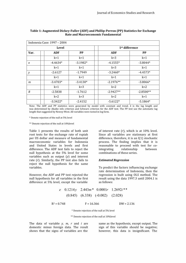
Table 1: Augmented Dickey-Fuller (ADF) and Phillip-Perron (PP) Statistics for ExchangeRate and Macroeconomic Fundamental

Indonesia Case: 1997 – 2004

Level 1st difference

Var. ADF PP ADF PP

k=1 k=1 k=3 k=1

e -4.4634* -3.1982* -4.1555* -3.8044*

k=1 k=1 k=3 k=1

y -2.6127 -1.7949 -3.2460* -4.4573*

k=1 k=1 k=1 k=1

m -3.4703* -3.4130* -2.1976** -3.8066*

k=1 k=3 k=2 k=2

R -2.5838 -1.7612 -2.9427** -2.8500**

k=2 k=3 k=2 k=1

-3.3422* -2.4152 -5.6122* -5.1864*Note: The ADF and PP statistics were generated by model with constant and trend. k is the lag length andwas determined by Akaike info criterion and Schwarz criterion for the ADF test. The PP test use the automatic laglength that suggested by Newey-West. All variables were tested in log form.

* Denote rejection of the null at 5% level

** Denote rejection of the null at 10%level

Table 1 presents the results of both unitroot tests for the exchange rate of rupiahper US dollar and measure of fundamentalmacroeconomic variables for Indonesiaand United States in levels and firstdifference. The ADF test fails to reject thenull hypothesis at the 5% level for somevariables such as output (y) and interestrate (r). Similarly, the PP test also fails toreject the null hypothesis for the samevariables.

However, the ADF and PP test rejected thenull hypothesis for all variables in the firstdifference at 5% level, except the variable

of interest rate (r), which is at 10% level.Since all variables are stationary at firstdifference, therefore, it is an I(1) stochasticprocess. The finding implies that it isreasonable to proceed with test for co-integrating relationship betweencombinations of these series.

Estimated Regression

To predict the factors influencing exchangerate determination of Indonesia, then theregression is built using OLS method. Theresult using the data 1997.3 until 2004.1 isas follows:

e 0.1214y

(0.845)

2.443m *

(6.338)

0.0001r

(-0.002)

1.2692i **

(2.028)

R2 = 0.748 F = 16.366 DW = 2.136

* Denote rejection of the null at 5% level

** Denote rejection of the null at 10%level

The data of variable y, m, r and i aredomestic minus foreign data. The resultshows that the signs of variables are the

same as the hypothesis, except output. Thesign of this variable should be negative;however, this data is insignificant. The


other variable that is insignificant isinterest rate, but it has the right sign. Theimplication of this finding is the interestrate is not a proper instrument in order toinfluence the exchange rate. When thecentral bank of Indonesia increases theinterest rate will only make the exchangerate appreciate a little bit, and it isinsignificant.

Money supply and price are significant ininfluencing the exchange rate of Indonesia.The increase of money supply and interestrate makes the exchange rate depreciate.An increase 1.0 percent of the moneysupply in Indonesia will depreciatebetween rupiah to 2.4 percent. This meansrupiah is very sensitive to the moneysupply. The implication of this finding isthe central bank has to control theexchange rate in order to stabilize therupiah.

The results reveal that the elasticityobtained for relative money supply m isgreater than unity (2.443). It indicates thatone-percent increase in Indonesia’srelative money supply will cause a long-rundepreciation of the rupiah by 2.443%, a

result consistent with overshootinghypothesis.

Price is also significant influencing theexchange rate. Indonesia’s inflation in 1998has been worsening the exchange rate. Anincrease 1.0 percent of inflation willstimulate depreciation of rupiah about 1.2percent.

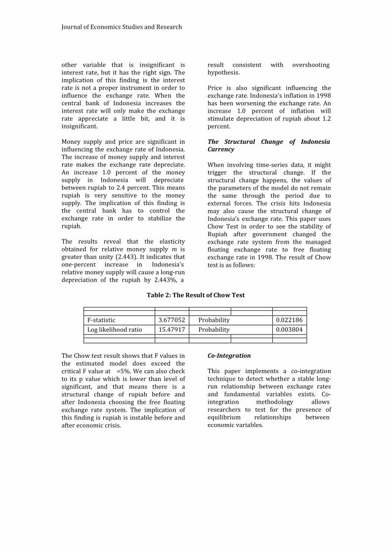
The Structural Change of IndonesiaCurrency

When involving time-series data, it mighttrigger the structural change. If thestructural change happens, the values ofthe parameters of the model do not remainthe same through the period due toexternal forces. The crisis hits Indonesiamay also cause the structural change ofIndonesia’s exchange rate. This paper usesChow Test in order to see the stability ofRupiah after government changed theexchange rate system from the managedfloating exchange rate to free floatingexchange rate in 1998. The result of Chowtest is as follows:

Table 2: The Result of Chow Test

F-statistic 3.677052 Probability 0.022186

Log likelihood ratio 15.47917 Probability 0.003804

The Chow test result shows that F values inthe estimated model does exceed thecritical F value at =5%. We can also checkto its p value which is lower than level ofsignificant, and that means there is astructural change of rupiah before andafter Indonesia choosing the free floatingexchange rate system. The implication ofthis finding is rupiah is instable before andafter economic crisis.

Co-Integration

This paper implements a co-integrationtechnique to detect whether a stable long-run relationship between exchange ratesand fundamental variables exists. Co-integration methodology allowsresearchers to test for the presence ofequilibrium relationships betweeneconomic variables.


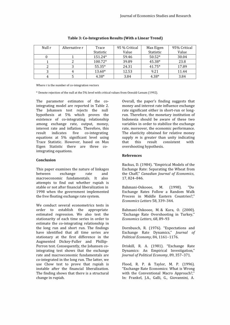
Table 3: Co-Integration Results (With a Linear Trend)

Null r Alternative r TraceStatistic

95 % CriticalValue

Max EigenStatistic

95% CriticalValue

0 1 151.24* 59.46 50.52* 30.041 2 100.72* 39.89 45.38* 23.82 3 55.35* 24.31 41.75* 17.893 4 13.60* 12.53 9.21 11.444 5 4.38* 3.84 4.38* 3.84

Where r is the number of co-integration vectors

* Denote rejection of the null at the 5% level with critical values from Oswald-Lenum (1992).

The parameter estimates of the co-integrating model are reported in Table 2.The Johansen test rejects the nullhypothesis at 5% which proves theexistence of co-integrating relationshipamong exchange rate, output, money,interest rate and inflation. Therefore, thisresult indicates five co-integratingequations at 5% significant level usingTrace Statistic. However, based on MaxEigen Statistic there are three co-integrating equations.

Conclusion

This paper examines the nature of linkagesbetween exchange rate andmacroeconomic fundamentals. It alsoattempts to find out whether rupiah isstable or not after financial liberalization in1998 when the government implementedthe free floating exchange rate system.

We conduct several econometrics tests inorder to establish the appropriateestimated regression. We also test thestationarity of each time series in order toestimate the co-integrating relationship inthe long run and short run. The findingshave identified that all time series arestationary at the first difference in theAugmented Dickey-Fuller and Phillip-Perron test. Consequently, the Johansen co-integrating test shows that the exchangerate and macroeconomic fundamentals areco-integrated in the long run. The latter, weuse Chow test to prove that rupiah isinstable after the financial liberalization.The finding shows that there is a structuralchange in rupiah.

Overall, the paper’s finding suggests thatmoney and interest rate influence exchangerate significant either in short-run or long-run. Therefore, the monetary institution ofIndonesia should be aware of these twovariables in order to stabilize the exchangerate, moreover, the economic performance.The elasticity obtained for relative moneysupply m is greater than unity indicatingthat this result consistent withovershooting hypothesis.

References

Backus, D. (1984). “Empirical Models of theExchange Rate: Separating the Wheat fromthe Chaff,” Canadian Journal of Economics,17, 824–846.

Bahmani-Oskooee, M. (1998). “DoExchange Rates Follow a Random WalkProcess in Middle Eastern Countries?,”Economics Letters 58, 339–344.

Bahmani-Oskooee, M. & Kara, O. (2000).“Exchange Rate Overshooting in Turkey,”Economics Letters, 68, 89–93

Dornbusch, R. (1976). “Expectations andExchange Rate Dynamics,” Journal ofPolitical Economy, 84, 1161–1176.

Driskill, R. A. (1981). “Exchange RateDynamics: An Empirical Investigation,”Journal of Political Economy, 89, 357–371.

Flood, R. P. & Taylor, M. P. (1996).“Exchange Rate Economics: What is Wrongwith the Conventional Macro Approach?,”In: Frankel, J.A., Galli, G., Giovannini, A.


(Eds.), Micro Structure of Foreign ExchangeMarkets, The University of Chicago Press.

Frankel, J. A. (1979). “On the Mark: ATheory of Floating Exchange Rate Based onReal Interest Differentials,” AmericanEconomic Review, 69, 610–627.

Hairault, J. O., Patureau, L. & Sopraseuth, T.(2004). “Overshooting and the ExchangeRate Disconnect Puzzle: A Reappraisal,”Journal of International Money and Finance,23, 615–643

Kim, S. & Roubini, N. (2000). “ExchangeRate Anomalies in the Industrial Countries:A Solution with a Structural VARApproach,” Journal of Monetary Economics,45, 561–586.

MacDonald, R. & Taylor, M. P. (1993). “TheMonetary Approach to the Exchange Rate,”IMF Stafff Papers, 40, 89–107.

Obstfeld, M. & Rogoff, K. (2000). “The SixMajor Puzzles in InternationalMacroeconomics: Is there a CommonCause?,” In: Bernanke, B., Rogoff, K. (Eds.),N.B.E.R Macroeconomic Annual 2000. MITPress, Cambridge, MA, 339–390.

Papel, D. H. (1988). “Expectations andExchange Rate Dynamics after a Decade ofFloating,” Journal of InternationalEconomics, 25, 303–317.

Education

The Linkages of Financial Liberalization and Currency Stability: What do we learn from Pre and Post Asian Financial Crisis?