Embed Size (px)
Citation preview

THE LINEAR PROGRAMMING APPROACH TO
APPROXIMATE DYNAMIC PROGRAMMING:
THEORY AND APPLICATION
a dissertation
submitted to the department of management science and engineering
and the committee on graduate studies
of stanford university
in partial fulfillment of the requirements
for the degree of
doctor of philosophy
Daniela Pucci de Farias
June 2002

c© Copyright by Daniela Pucci de Farias 2002
All Rights Reserved
ii

I certify that I have read this dissertation and that, in
my opinion, it is fully adequate in scope and quality as a
dissertation for the degree of Doctor of Philosophy.
Benjamin Van Roy(Principal Adviser)
I certify that I have read this dissertation and that, in
my opinion, it is fully adequate in scope and quality as a
dissertation for the degree of Doctor of Philosophy.
Peter Glynn
I certify that I have read this dissertation and that, in
my opinion, it is fully adequate in scope and quality as a
dissertation for the degree of Doctor of Philosophy.
Arthur Veinott, Jr.
Approved for the University Committee on Graduate
Studies:
iii

iv
Abstract
Dynamic programming offers a unified approach to solving problems of stochastic
control. Central to the methodology is the optimal value function, which can be
obtained via solving Bellman’s equation. The domain of the optimal value function is
the state space of the system to be controlled, and dynamic programming algorithms
compute and store a table consisting of the optimal value function evaluated at each
state. Unfortunately, the size of a state space typically grows exponentially in the
number of state variables. Known as the curse of dimensionality, this phenomenon
renders dynamic programming intractable in the face of problems of practical scale.
Approximate dynamic programming aims to alleviate the curse of dimensionality
by considering approximations to the optimal value function — scoring functions —
that can be computed and stored efficiently. For instance, one might consider gener-
ating an approximation within a parameterized class of functions, in a spirit similar
to that of statistical regression. The focus of this dissertation is on an algorithm for
computing parameters for linearly parameterized function classes. We study approx-
imate linear programming, an algorithm based on a linear programming formulation
that generalizes the linear programming approach to exact dynamic programming.
Over the years, interest in approximate dynamic programming has been fueled by
stories of empirical success in application areas spannning from games to dynamic re-
source allocation to finance . Nevertheless, practical use of the methodology remains
limited by a lack of systematic guidelines for implementation and theoretical guaran-
tees, which reflects on the amount of trial and error involved in each of the success
stories found in the literature and on the difficulty of duplicating the same success
in other applications. The research presented in this dissertation addresses some of
v

these issues. In particular, our analysis leads to theoretically motivated guidelines for
implementation of approximate linear programming.
Specific contributions of this dissertation can be described as follows:
• We offer bounds that characterize the quality of approximations produced by
the linear programming approach and the quality of the policy ultimately gen-
erated. In addition to providing performance guarantees, the error bounds and
associated analysis offer new interpretations and insights pertaining to the lin-
ear programming approach. Among other things, this understanding to some
extent guides selection of basis functions and “state-relevance weights” that
influence quality of the approximation.
• Approximate linear programming involves solution of linear programs with rel-
atively few variables but an intractable number of constraints. We propose a
constraint sampling scheme that retains and uses only a tractable subset of the
constraints. We show that, under certain assumptions, the resulting approxi-
mation is comparable to the solution that would be generated if all constraints
were taken into consideration.
• Some of the theoretical results are illustrated in applications to queueing prob-
lems. We also devote a chapter to case studies that demonstrate practical as-
pects of implementation of approximate linear programming to queueing prob-
lems and web server farm management and demonstrate effectiveness of the
methodology in problems of relevance to industry.
vi

Preface
Few problems are more universal than that of sequential decision-making under un-
certainty. To shape one’s actions to balance present and future consequences is life’s
ever-standing challenge, and the ability to successfully navigate through the over-
whelmingly large tree of possibilities what might be regarded as the art of the wise.
What, then, constitutes wisdom? How does one not become paralyzed in the
analysis of all possible scenarios, but make good moves with limited consideration
instead? What does good even mean in this setting?
In life, the ability to make good decisions lies to a large extent in the ability to
see the forest through the trees. When the mapping from actions to consequences is
nontrivial and exhaustive search through all possible scenarios is prohibitively expen-
sive, clarity of thought allows one to filter out unnecessary details and identify the
main factors at play, reducing the problem complexity.
Although not quite as fascinating as life’s most pressing issues, many problems in
engineering, science and business pose similar challenges: a large number of scenar-
ios and options, uncertainty about the future, and nontrivial mapping from actions
to consequences. This dissertation is part of an effort toward the understanding of
decision-making in such problems; toward the development of a unified theory of con-
trol of complex systems. In other words, toward the development of the mathematical
and algorithmic equivalent of wisdom.
vii

viii

Acknowledgments
My thesis advisor Prof. Ben Van Roy had immense impact on my research philosophy
and style. I am grateful to him for passing on to me strong ethical values, appreciation
for elegant work and the willingness to set ambitious research goals. The research
presented in this dissertation is the fruit of a close collaboration and would certainly
not have been the same without his invaluable contribution.
I am also thankful to my dissertation readers Professors Peter Glynn and Arthur
Veinott Jr. and defense committee members Professors Daphne Koller and David
Luenberger for valuable comments and suggestions.
Section 6.2 represents joint work with Drs. Alan King and Mark Squillante, as
well as Dave Mulford. The fluid model approximation for the problems of scheduling
and routing is due to Drs. Zhen Liu, Mark Squillante and Joel Wolf. The model for
arrival rate processes was based on discussions with Dr. Ta-Hsin Lee.
My education at Stanford was enriched by interaction with fellow students. I
would like to thank David Choi, Eric Cope, Kahn Mason, Dave Mulford, Shikhar
Ranjan, Paat Rusmevichientong and Peter Salzman for great discussions on various
research subjects.
I thank my family for unconditional support throughout the years. They provided
everything I needed to succeed. Eduardo Cheng was also a fundamental source of
support in my early years at Stanford. Discussions with my master’s thesis advisor
Prof. Jose Claudio Geromel in my early undergraduate and master’s years played a
fundamental role in shaping my career path. He has also been a permanent source of
support and encouragement.
Through the days and through the nights, little Francisca was there for me. She
ix

never uttered a word of discouragement, and was always cheerful and willing to endure
long hours of work with me. Life as a researcher would not be the same without the
lovely sight of her lying in the corner of the room, walking on the keyboard, or happily
eating my papers.
This research was supported by a Stanford School of Engineering Fellowship, a
Wells Fargo Bank Fellowship, a Stoloroff Fellowship, an IBM Research Fellowship,
the NSF CAREER Grant ECS-9985229, and the ONR under Grant MURI N00014-
00-1-0637.
x

To the loving memory of Sissi,
and to adorable Francisca.
xi

xii
Contents
Abstract v
Preface vii
Acknowledgments ix
1 Introduction 1
1.1 Complex Systems . . . . . . . . . . . . . . . . . . . . . . . . . . . . . 1
1.2 Approximate Dynamic Programming . . . . . . . . . . . . . . . . . . 3
1.3 Approximation Architectures . . . . . . . . . . . . . . . . . . . . . . . 4
1.4 Approximate Linear Programming . . . . . . . . . . . . . . . . . . . . 6
1.5 Some History . . . . . . . . . . . . . . . . . . . . . . . . . . . . . . . 8
1.6 Chapter Organization and Contributions . . . . . . . . . . . . . . . . 9
2 Approximate Linear Programming 13
2.1 Markov Decision Processes . . . . . . . . . . . . . . . . . . . . . . . . 13
2.2 Approximate Dynamic Programming . . . . . . . . . . . . . . . . . . 17
2.3 Approximate Linear Programming . . . . . . . . . . . . . . . . . . . . 20
3 State-Relevance Weights 23
3.1 State-Relevance Weights in the Approximate LP . . . . . . . . . . . . 24
3.2 On The Quality of Policies Generated by ALP . . . . . . . . . . . . . 25
3.3 Heuristic Choices of State-Relevance Weights . . . . . . . . . . . . . . 28
3.3.1 States with Very Large Costs . . . . . . . . . . . . . . . . . . 29
xiii
3.3.2 Weights Induced by Steady-State Probabilities . . . . . . . . . 32
3.4 Closing Remarks . . . . . . . . . . . . . . . . . . . . . . . . . . . . . 35
4 Approximation Error Analysis 37
4.1 A Graphical Interpretation of ALP . . . . . . . . . . . . . . . . . . . 38
4.2 A Simple Bound . . . . . . . . . . . . . . . . . . . . . . . . . . . . . . 39
4.3 An Improved Bound . . . . . . . . . . . . . . . . . . . . . . . . . . . 41
4.4 On the Choice of Lyapunov Function . . . . . . . . . . . . . . . . . . 47
4.4.1 An Autonomous Queue . . . . . . . . . . . . . . . . . . . . . . 47
4.4.2 A Controlled Queue . . . . . . . . . . . . . . . . . . . . . . . 51
4.4.3 A Queueing Network . . . . . . . . . . . . . . . . . . . . . . . 54
4.5 At the Heart of Lyapunov Functions . . . . . . . . . . . . . . . . . . 57
5 Constraint Sampling 65
5.1 Relaxing the Approximate LP Constraints . . . . . . . . . . . . . . . 66
5.2 High-Confidence Sampling for Linear Constraints . . . . . . . . . . . 71
5.2.1 Uniform Convergence of Empirical Probabilities . . . . . . . . 74
5.3 High-Confidence Sampling and ALP . . . . . . . . . . . . . . . . . . 77
5.3.1 Bounding Constraint Violations . . . . . . . . . . . . . . . . . 83
5.3.2 Choosing the Constraint Sampling Distribution . . . . . . . . 88
5.3.3 Dealing with Large Action Spaces . . . . . . . . . . . . . . . . 89
5.4 Closing Remarks . . . . . . . . . . . . . . . . . . . . . . . . . . . . . 91
6 Case Studies 93
6.1 Queueing Problems . . . . . . . . . . . . . . . . . . . . . . . . . . . . 93
6.1.1 Single Queue with Controlled Service Rate . . . . . . . . . . . 94
6.1.2 A Four-Dimensional Queueing Network . . . . . . . . . . . . . 97
6.1.3 An Eight-Dimensional Queueing Network . . . . . . . . . . . . 98
6.2 Web Server Farm Management . . . . . . . . . . . . . . . . . . . . . 101
6.2.1 Problem Formulation . . . . . . . . . . . . . . . . . . . . . . . 102
6.2.2 Solving the Scheduling and Routing Problems . . . . . . . . . 104
6.2.3 The Arrival Rate Process . . . . . . . . . . . . . . . . . . . . . 108
xiv
6.2.4 An MDP Model for the Web Server Allocation Problem . . . . 108
6.2.5 Dealing with State Space Complexity . . . . . . . . . . . . . . 109
6.2.6 Dealing with Action Space Complexity . . . . . . . . . . . . . 114
6.2.7 Experimental Results . . . . . . . . . . . . . . . . . . . . . . . 115
6.2.8 Closing Remarks . . . . . . . . . . . . . . . . . . . . . . . . . 117
7 Conclusions 121
Bibliography 125
xv

xvi
Chapter 1
Introduction
Problems of sequential decision-making in complex systems are a recurrent theme in
engineering, science and business. Optimal control of such systems typically requires
consideration of a large number of scenarios and options and treatment of uncertainty
surrounding future events. Some problems exhibit special structure that allows one
to circumvent the apparent complexity and achieve optimality efficiently; however,
for the vast majority of applications, optimality remains an impossible goal in face of
current computing power limitations. How to make good decisions efficiently in such
applications is the subject of this dissertation.
1.1 Complex Systems
We defer a formal characterization of complex systems to Chapter 2. Loosely de-
scribed, the complexity of a system is determined by certain features that may in-
fluence how difficult it is to design optimal control strategies. Features that have an
impact include the complexity of the system dynamics (linear/nonlinear); the pres-
ence or absence of uncertainty; the number of scenarios and options being considered.
We now present instances of control problems involving complex systems, illustrating
the impact of some of these features on the decision-making process.
Example 1.1 Scheduling in manufacturing systems
Consider a plant used for the manufacturing of several different types of products.
1
2 CHAPTER 1. INTRODUCTION
Each product is characterized by a sequence of processing steps. Machines in this
plant may perform multiple functions, such as several processing steps for a given
product, or processing steps for several different products. Managing such systems
requires scheduling each machine to share its time among the several jobs waiting in
queue for service. This is done with some objective in mind; common choices are to
maximize production rates (throughput) or minimize the number of unfinished units
in the system. Since jobs travel from machine to machine, there is usually a high
degree of interconnectivity in manufacturing systems, and optimality requires joint
consideration of the status of all queues in the system and of the decisions being made
for all machines, leading to difficulties as the system dimensions increase.
Example 1.2 Zero-sum games
Zero-sum games involve two agents playing with completely opposed objectives: the
gain of one agent is the loss of the other. An example of a zero-sum game is chess.
An optimal strategy for playing chess requires investigation of all possible moves for
the current step, investigation of all subsequent moves for the adversary, and so on,
until completion of the game, so that one can choose the move that maximizes the
chance of victory. Given the large number of moves available for each player and the
large number of configurations the chess board can take, this approach is infeasible:
consideration of even four or five moves into the future leads to a huge number of
possibilities.
Example 1.3 Dynamic portfolio allocation
Consider the problem of deciding what fraction of current capital to invest in each
of multiple stocks available in the market. A fraction of the money is devoted to
consumption, and the objective is to maximize the sum of a utility of consumption
over time. Stock prices follow particularly complicated dynamics, being affected by
uncertainty and by a large number of factors in the market. Optimality in the long
run would require consideration of the joint evolution of all these factors, as they
are generally interdependent. This is intractable unless only a very small number of
factors is considered in the stock price model.
1.2. APPROXIMATE DYNAMIC PROGRAMMING 3
1.2 Approximate Dynamic Programming
A common approach to decision-making in complex systems is the heuristic approach.
Much like what one would do in life, when confronted with such systems one tries
to identify ways of simplifying the problem to make it solvable while still capturing
its essence. Heuristics exploit the best of human capacity — creativity — and work
surprisingly well at times. However, they also have to be reinvented with each new
application, as in general little knowledge is reused when one switches between appli-
cations which are far apart in scope, for example, from scheduling in manufacturing
systems to chess. A strong focus on deriving simple rules of thumb, which is common
in problem-specific approaches, may also lead to inefficient use of a valuable resource:
computers’ power to perform a large number of operations fast and accurately.
Dynamic programming offers a unified treatment of a wide variety of problems
involving sequential decision-making in systems with nonlinear, stochastic dynamics.
Systems in this setting are described by a collection of variables evolving over time —
the state variables. State variables take values in the state space of the system, the set
of all possible states the system can be in. The central idea in dynamic programming is
that, for a variety of optimality criteria, optimal decisions can be derived from a score
assigned to each of the different states in the system. The optimal scoring function
prescribed by dynamic programming is referred to as the optimal value function, and
it captures the advantage of being in a given state relative to being in others.
Unfortunately, the applicability of dynamic programming is severely limited by
the curse of dimensionality: computing and storing the optimal value function over
the entire state space requires time and space exponential in the number of state vari-
ables. Hence for most problems of practical interest, dynamic programming remains
computationally infeasible.
Approximate dynamic programming tries to combine the best elements of the
heuristic and the dynamic programming approaches. It draws on traditional dynamic
programming concepts and techniques to derive appropriate scoring functions. How-
ever, differently from dynamic programming, the emphasis is not on global optimality,
but rather on doing well given computational limitations. In approximate dynamic
4 CHAPTER 1. INTRODUCTION
programming, this translates into finding scoring functions that can be computed and
stored efficiently. The underlying assumption is that many problems of practical in-
terest exhibit some structure leading to the existence of reasonable scoring functions
that can be represented compactly. Algorithms drawing on dynamic programming
concepts and simultaneously exploiting problem-specific structure would hopefully
combine the generality of dynamic programming and the efficiency of heuristics.
We refer to the general structure one assumes for the scoring function as the
approximation architecture. Approximation architectures are one of the two central
themes of research in approximate dynamic programming. The other central theme
relates to algorithms for finding a good scoring function within the architecture under
consideration.
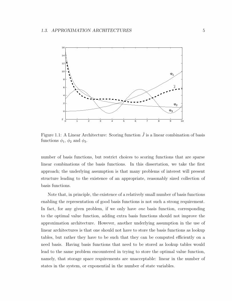
1.3 Approximation Architectures
An appropriate choice of approximation architecture is essential for successful use
of approximate dynamic programming: a scoring function can only be as good as
the approximation architecture that defines its structure. In this dissertation, we
consider the use of linear architectures. In a spirit reminiscent of linear regression,
one chooses a collection of functions mapping the system state space to real numbers
— the basis functions — and generates a scoring function by finding an appropriate
linear combination of these basis functions. Note that the architecture is called linear
because we look for scoring functions that are linear in the basis functions; in principle,
the basis functions are arbitrary functions of the system state. Figure 1.1 illustrates
the use of basis functions in generating a scoring function.
A scoring function representable as a linear combination of basis functions is fully
characterized by the weights assigned to each of the basis functions in this linear
combination. Hence it suffices to store these weights (one per basis function) as an
encoding of the scoring function. In contrast, the optimal value function typically
requires representation as a lookup table, with one value per state in the system. The
use of a linear approximation architecture will therefore be feasible and advantageous
if either we have only a manageable number of basis functions or we have a large
1.3. APPROXIMATION ARCHITECTURES 5
0 1 2 3 4 5 6 7 8 9 102
0
2
4
6
8
10
12
14
16
φ1
φ2
φ3
J~
Figure 1.1: A Linear Architecture: Scoring function J is a linear combination of basisfunctions φ1, φ2 and φ3.
number of basis functions, but restrict choices to scoring functions that are sparse
linear combinations of the basis functions. In this dissertation, we take the first
approach; the underlying assumption is that many problems of interest will present
structure leading to the existence of an appropriate, reasonably sized collection of
basis functions.
Note that, in principle, the existence of a relatively small number of basis functions
enabling the representation of good basis functions is not such a strong requirement.
In fact, for any given problem, if we only have one basis function, corresponding
to the optimal value function, adding extra basis functions should not improve the
approximation architecture. However, another underlying assumption in the use of
linear architectures is that one should not have to store the basis functions as lookup
tables, but rather they have to be such that they can be computed efficiently on a
need basis. Having basis functions that need to be stored as lookup tables would
lead to the same problem encountered in trying to store the optimal value function,
namely, that storage space requirements are unacceptable: linear in the number of
states in the system, or exponential in the number of state variables.
6 CHAPTER 1. INTRODUCTION
The practical limitations on the complexity of the basis functions also imply that,
although in principle linear architectures are rich enough, in practice it may be worth
exploring different approximation architectures as well. Common choices are neural
networks [7, 25], or splines [50, 11]. A potential drawback in the use of nonlinear
architectures is that algorithms for finding appropriate scoring functions with such a
structure are usually more complicated.
1.4 Approximate Linear Programming
Given a prespecified linear architecture, we must be able to identify an appropriate
scoring function among all functions that are representable as linear combinations of
the basis functions. In approximate dynamic programming, it is natural to define the
quality of the scoring function in terms of its closeness to the optimal value function.
Therefore an ideal algorithm might try to choose the linear combination of basis
functions that minimizes some distance to the optimal value function. Note that this
is the main idea in traditional regression problems, where one tries to fit a curve based
on noisy observations by minimizing, for example, the sum of the squared errors over
the samples. Unfortunately, the same idea cannot be applied in the approximate
dynamic programming setting because we cannot sample the optimal value function.
Alternatively, we seek inspiration in standard dynamic programming algorithms
to derive scoring functions that will hopefully serve as good substitutes to the optimal
value function. Approximate dynamic programming algorithms are typically adap-
tations of standard dynamic programming algorithms that are changed to account
for the use of an approximation architecture. Approximate linear programming, the
method studied here, falls in that category.
Approximate linear programming is inspired by the more traditional linear pro-
gramming approach to exact dynamic programming [9, 17, 18, 19, 26, 34]. Perhaps
quite surprisingly, even though dynamic programming problems involve optimization
of fairly arbitrary functionals, they can be recast as linear programs (LP’s). However,
these LP’s are not immune the curse of dimensionality: they have as many variables
as the number of states in the system, and at least the same number of constraints.
1.4. APPROXIMATE LINEAR PROGRAMMING 7
Combining the linear programming approach to exact dynamic programming with
linear approximation architectures leads to the approximate linear programming al-
gorithm (ALP), originally proposed by Schweitzer and Seidmann [43]. ALP involves
the use of an LP with reduced dimensions to generate a scoring function. We call
this LP the approximate LP. Compared with the exact LP that computes the optimal
value function, the approximate LP will typically have a much smaller number of vari-
ables: it has as many variables as the number of basis functions. A potential source of
concern is that the approximate LP still has a huge number of constraints, in fact as
many as those present in the exact LP. However, LP’s presenting few variables and a
large number of constraints are good candidates to constraint generation techniques.
Specifically, we show in the approximate linear programming case how an efficient
constraint sampling mechanism can be designed for achieving good approximations
to the approximate LP solution in reasonable time.
Compared to other approximate dynamic programming algorithms, approximate
linear programming offers some advantages:
• Approximate linear programming capitalizes on decades of research on linear
programming. Heavy use of such a standard methodology implies that imple-
mentation of the approximate LP may be easier to non-experts than implemen-
tation of other methods would be. Combined with the fact that one can take
advantage of the several large-scale linear programming algorithms available,
this leads to a higher likelihood of approximate linear programming effectively
becoming a useful method in industry.
• In the case of minimizing costs (maximizing rewards), approximate linear pro-
gramming offers a lower (upper) bound on the optimal long-run costs (rewards).
Upper (lower) bounds can be generated fairly easily by simulation of any pol-
icy. Therefore, there is a possibility of identifying from the approximate linear
programming solution whether the chosen linear architecture is satisfactory or
further refinements may lead to substantial improvement in performance.
• The inherent simplicity of linear programming implies that approximate lin-
ear programming is relatively easier to analyze than some other approximate
8 CHAPTER 1. INTRODUCTION
dynamic programming algorithms. A great obstacle in making approximate dy-
namic programming popular is that, apart from anecdotal success, it has been
difficult to demonstrate strong guarantees for such methods, and to fully un-
derstand their behavior. A characteristic common to all approximate dynamic
programming methods is that their behavior depends on many different algo-
rithm parameters. With little understanding of how each of the parameters
affects the overall quality of the method, appropriately setting them typically
requires a large amount of trial and error, and there is a high probability of
failure in identifying adequate values. While this problem is not fully solved in
approximate linear programming, there is a deeper understanding of the impact
of its parameters in the ultimate scoring function being generated. Analysis such
as that presented in this dissertation provides valuable guidance in the choice of
algorithm parameters and increases the probability of successful implementation
of the method.
1.5 Some History
Perhaps one of the earliest developments in the area of automated decision-making
in complex systems is due to Shannon, in a paper that proposes an algorithm for
playing chess [44]. The paper suggests the use of scoring functions for assessing the
many different board configurations a move can lead to. The scoring function should
represent an assessment of long-run rewards associated with each board configuration.
Scores were based on a linear combination of certain features of the board configura-
tion empirically known to be relevant to the game. Both the features and the linear
combination thereof used as a scoring function were chosen heuristically. The idea of
using scoring functions for assessing board configuration forms the basis for modern
chess playing projects.
Concern with the curse of dimensionality and research on approximate dynamic
programming was a part of early research on dynamic programming. Belmann re-
ferred to such algorithms, aiming to the design of scoring functions to serve as ap-
proximations to the optimal value function, as approximations in the value space [3].
1.6. CHAPTER ORGANIZATION AND CONTRIBUTIONS 9
However, despite early efforts, relatively modest progress was made until the recent
renaissance of the field in the artificial intelligence domain. Successful implementation
of reinforcement learning algorithms, most notably the development of a world-class
automatic backgammon player [48], generated great interest in the methodology and
inspired further research in the area. Later analysis of reinforcement learning re-
vealed strong connections with dynamic programming: the algorithm corresponds to
a stochastic, approximate version of value and policy iteration, traditional dynamic
programming algorithms. Unfortunately, reinforcement learning algorithms such as
temporal-difference learning remain largely unexplained, with the strongest guaran-
tees being limited to the cases of autonomous systems and optimal stopping problems
[51, 53, 52].
An alternative to approximate dynamic programming algorithms such as temporal-
difference learning or approximate linear programming is what are called approxima-
tions in the policy space. In such algorithms, instead of trying to derive a good policy
indirectly via generation of a scoring function, one aims to generating a sequence of
improving policies. Searching directly in the policy space typically requires consid-
eration of parametric policies. If the dependence of the optimality criterion (e.g.,
average cost) on the policy parameter is differentiable, one may be able to use gra-
dient descent methods to identify a policy corresponding to a local optimum within
the parametric class under consideration [1, 2, 35, 37, 58].
A more recent development combines approximation in the state space with ap-
proximation in the policy space. Actor-critic algorithms involve the use of both
parametric policies and value function approximation to generate a stochastic version
of policy iteration [46, 28, 27].
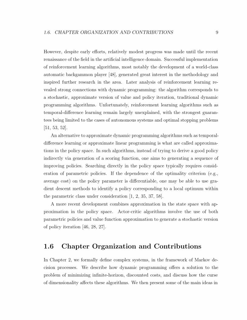
1.6 Chapter Organization and Contributions
In Chapter 2, we formally define complex systems, in the framework of Markov de-
cision processes. We describe how dynamic programming offers a solution to the
problem of minimizing infinite-horizon, discounted costs, and discuss how the curse
of dimensionality affects these algorithms. We then present some of the main ideas in
10 CHAPTER 1. INTRODUCTION
approximate dynamic programming and introduce approximate linear programming,
the algorithm studied in the remaining chapters.
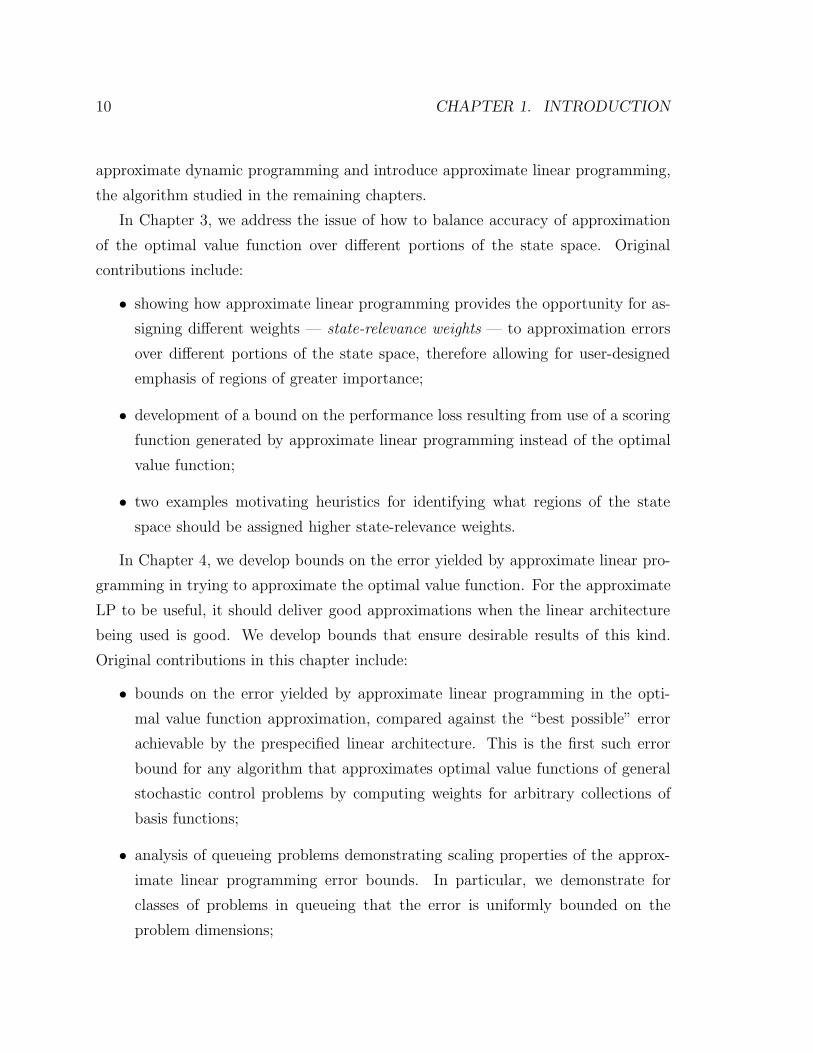
In Chapter 3, we address the issue of how to balance accuracy of approximation
of the optimal value function over different portions of the state space. Original
contributions include:
• showing how approximate linear programming provides the opportunity for as-
signing different weights — state-relevance weights — to approximation errors
over different portions of the state space, therefore allowing for user-designed
emphasis of regions of greater importance;
• development of a bound on the performance loss resulting from use of a scoring
function generated by approximate linear programming instead of the optimal
value function;
• two examples motivating heuristics for identifying what regions of the state
space should be assigned higher state-relevance weights.
In Chapter 4, we develop bounds on the error yielded by approximate linear pro-
gramming in trying to approximate the optimal value function. For the approximate
LP to be useful, it should deliver good approximations when the linear architecture
being used is good. We develop bounds that ensure desirable results of this kind.
Original contributions in this chapter include:
• bounds on the error yielded by approximate linear programming in the opti-
mal value function approximation, compared against the “best possible” error
achievable by the prespecified linear architecture. This is the first such error
bound for any algorithm that approximates optimal value functions of general
stochastic control problems by computing weights for arbitrary collections of
basis functions;
• analysis of queueing problems demonstrating scaling properties of the approx-
imate linear programming error bounds. In particular, we demonstrate for
classes of problems in queueing that the error is uniformly bounded on the
problem dimensions;
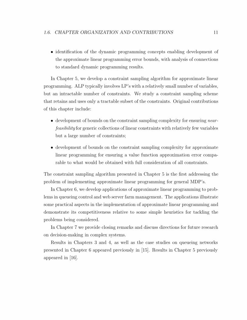
1.6. CHAPTER ORGANIZATION AND CONTRIBUTIONS 11
• identification of the dynamic programming concepts enabling development of
the approximate linear programming error bounds, with analysis of connections
to standard dynamic programming results.
In Chapter 5, we develop a constraint sampling algorithm for approximate linear
programming. ALP typically involves LP’s with a relatively small number of variables,
but an intractable number of constraints. We study a constraint sampling scheme
that retains and uses only a tractable subset of the constraints. Original contributions
of this chapter include:
• development of bounds on the constraint sampling complexity for ensuring near-
feasibility for generic collections of linear constraints with relatively few variables
but a large number of constraints;
• development of bounds on the constraint sampling complexity for approximate
linear programming for ensuring a value function approximation error compa-
rable to what would be obtained with full consideration of all constraints.
The constraint sampling algorithm presented in Chapter 5 is the first addressing the
problem of implementing approximate linear programming for general MDP’s.
In Chapter 6, we develop applications of approximate linear programming to prob-
lems in queueing control and web server farm management. The applications illustrate
some practical aspects in the implementation of approximate linear programming and
demonstrate its competitiveness relative to some simple heuristics for tackling the
problems being considered.
In Chapter 7 we provide closing remarks and discuss directions for future research
on decision-making in complex systems.
Results in Chapters 3 and 4, as well as the case studies on queueing networks
presented in Chapter 6 appeared previously in [15]. Results in Chapter 5 previously
appeared in [16].

12 CHAPTER 1. INTRODUCTION
Chapter 2
Approximate Linear Programming
Markov decision processes (MDP’s) provide a unified framework for the treatment of
problems of sequential decision-making under uncertainty. For a variety of optimality
criteria, these problems can be solved by dynamic programming. The main strength of
this approach is that fairly general stochastic and nonlinear dynamics can be consid-
ered. However, the same generality leads to poor use of problem-specific information
to guide the derivation of optimal policies, leading to efficiencies that are ultimately
unbearable — dynamic programming algorithms are computationally infeasible for
all but very small problems, or problems exhibiting very special structure.
In this chapter, we formally define complex systems, in the MDP framework. We
describe how dynamic programming offers a solution to the problem of minimizing
discounted costs over an infinite horizon, and discuss how the curse of dimensionality
affects dynamic programming algorithms. We then present some of the main ideas in
approximate dynamic programming and introduce approximate linear programming,
the algorithm studied in the remaining chapters.
2.1 Markov Decision Processes
In the MDP framework, systems are characterized by collections of variables evolving
over time — the state variables. State variables summarize the history of the system,
containing all information that is relevant to predicting future events. In formulating a
13
14 CHAPTER 2. APPROXIMATE LINEAR PROGRAMMING
problem as an MDP, state variables must be designed to satisfy the Markov property:
conditioned on the current state of the system being known, its future is independent
from its past. The Markov property has important implications in the search for
optimal policies, as we shall later see.
The evolution of state variables is partially dependent on decisions or controls
exogenous to the system. We consider the problem of determining such decisions so
as to minimize a discounted sum of costs incurred as the system runs ad infinitum.
We consider systems running in discrete time. Costs accrue at each time step and
depend on the state of the system and action being taken at that time.
We now provide a formal description of Markov decision processes. A Markov
decision process in discrete-time is characterized by a tuple
(S,A·, P·(·, ·), g·(·), α),
with the following interpretation. We consider stochastic control problems involving
a finite state space S of cardinality |S| = N . For each state x ∈ S, there is a finite
set of available actions Ax. When the current state is x and action a ∈ Ax is taken,
a cost ga(x) is incurred. State transition probabilities Pa(x, y) represent, for each
pair (x, y) of states and each action a ∈ Ax, the probability that the next state will
be y conditioned on the current state being x and the current action being a ∈ Ax.
The discount factor α is a scalar between zero and one and represents inter-temporal
preferences, indicating how costs incurred at different time steps are combined in a
single optimality criterion.
A policy is a mapping from states to actions. Given a policy u, the dynamics of
the system follow a Markov chain with transition probabilities Pu(x)(x, y). For each
policy u, we define a transition matrix Pu whose (x, y)th entry is Pu(x)(x, y).
For concreteness, let us consider an example.
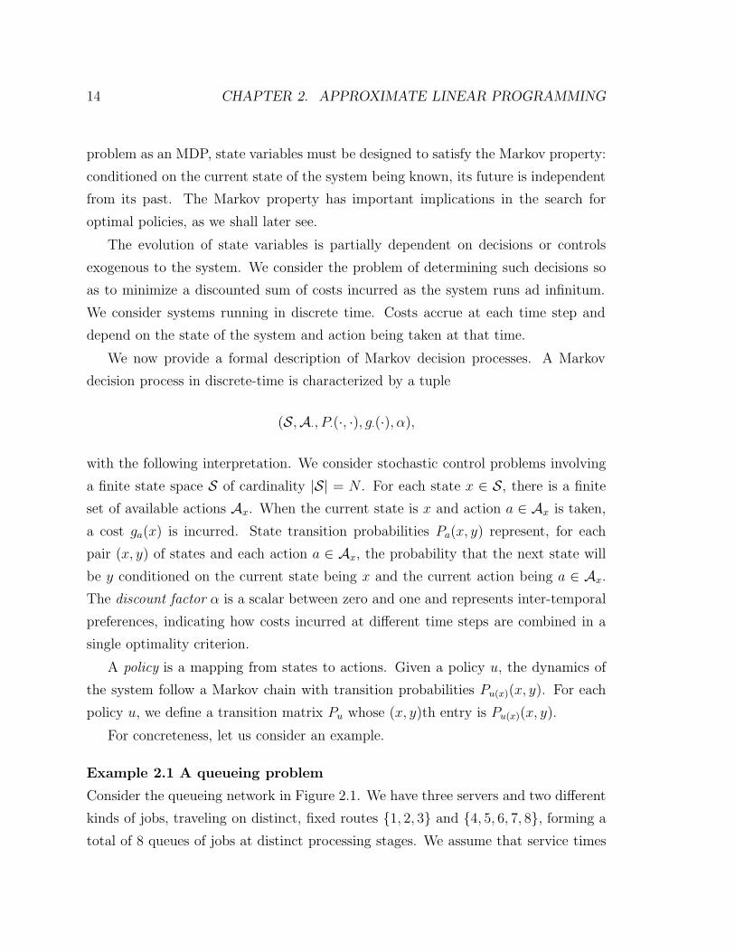
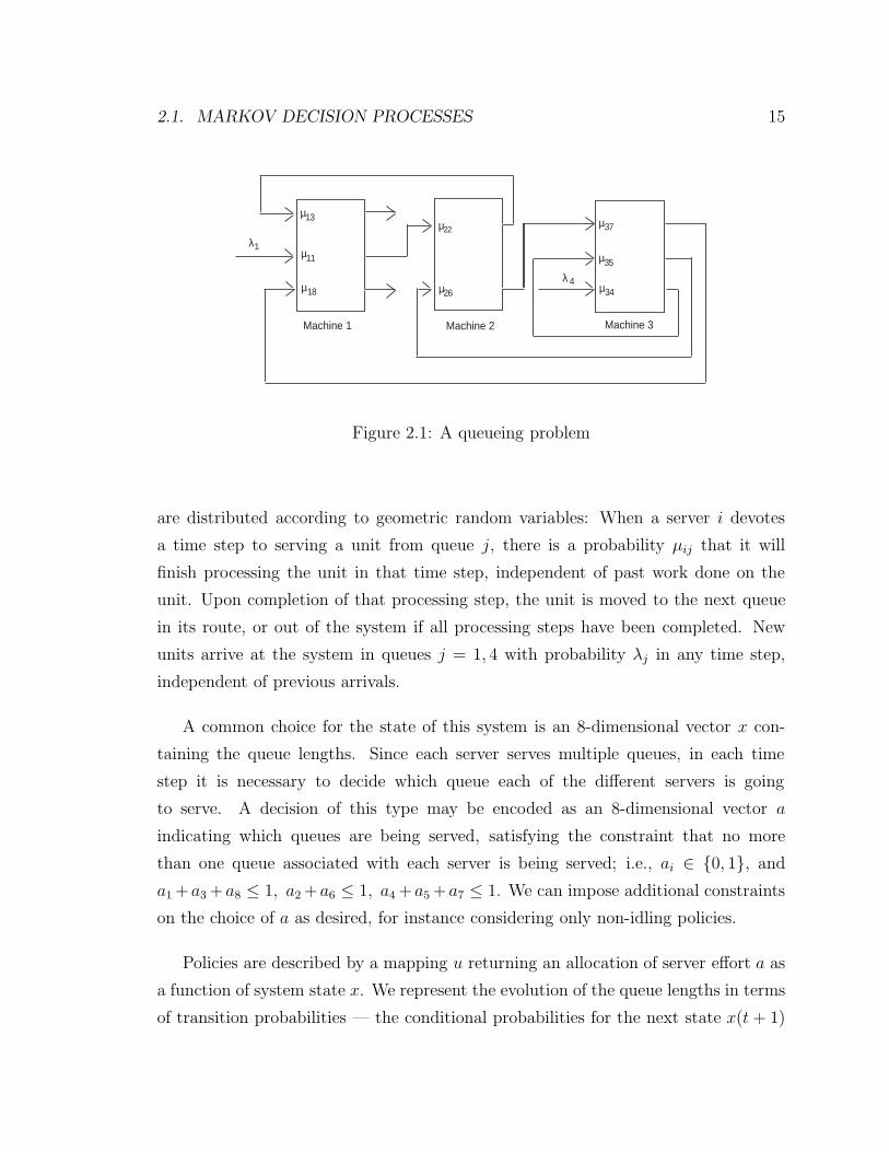
Example 2.1 A queueing problem
Consider the queueing network in Figure 2.1. We have three servers and two different
kinds of jobs, traveling on distinct, fixed routes {1, 2, 3} and {4, 5, 6, 7, 8}, forming a
total of 8 queues of jobs at distinct processing stages. We assume that service times
2.1. MARKOV DECISION PROCESSES 15
λ1
λ 4
µ11
µ18
µ13µ22
µ26 µ34
µ35
µ37
Machine 1 Machine 2 Machine 3
Figure 2.1: A queueing problem
are distributed according to geometric random variables: When a server i devotes
a time step to serving a unit from queue j, there is a probability µij that it will
finish processing the unit in that time step, independent of past work done on the
unit. Upon completion of that processing step, the unit is moved to the next queue
in its route, or out of the system if all processing steps have been completed. New
units arrive at the system in queues j = 1, 4 with probability λj in any time step,
independent of previous arrivals.
A common choice for the state of this system is an 8-dimensional vector x con-
taining the queue lengths. Since each server serves multiple queues, in each time
step it is necessary to decide which queue each of the different servers is going
to serve. A decision of this type may be encoded as an 8-dimensional vector a
indicating which queues are being served, satisfying the constraint that no more
than one queue associated with each server is being served; i.e., ai ∈ {0, 1}, and
a1 +a3 +a8 ≤ 1, a2 +a6 ≤ 1, a4 +a5 +a7 ≤ 1. We can impose additional constraints
on the choice of a as desired, for instance considering only non-idling policies.
Policies are described by a mapping u returning an allocation of server effort a as
a function of system state x. We represent the evolution of the queue lengths in terms
of transition probabilities — the conditional probabilities for the next state x(t+ 1)
16 CHAPTER 2. APPROXIMATE LINEAR PROGRAMMING
given that the current state is x(t) and the current action is a(t). For instance:
Prob (x1(t+ 1) = x1(t) + 1|x(t), a(t)) = λ1,
P rob (x3(t+ 1) = x3(t) + 1, x2(t+ 1) = x2(t)− 1|x(t), a(t))= µ22I(x2(t) > 0, a2(t) = 1),
P rob (x3(t+ 1) = x3(t)− 1, |x(t), a(t)) = µ13I(x3(t) > 0, a3(t) = 1),
corresponding to an arrival to queue 1, a departure from queue 2 and an arrival to
queue 3, and a departure from queue 3. I(.) is the indicator function. Transition
probabilities related to other events are defined similarly.
We consider costs of the form g(x) =∑
i xi, the total number of unfinished units in
the system. For instance, this is a reasonably common choice of cost for manufacturing
systems, which are often modeled as queueing networks.
The problem of stochastic control amounts to selection of a policy that optimizes
a given criterion. We employ as an optimality criterion infinite-horizon discounted
cost of the form
Ju(x) = E
[ ∞∑t=0
αtgu(xt)∣∣∣x0 = x
], (2.1)
where gu(x) is used as shorthand for gu(x)(x) and the discount factor α ∈ (0, 1) reflects
inter-temporal preferences. In finance problems, α has a concrete interpretation: the
same nominal value is worth less in the future than in the present, since in the latter
case it can be invested for a risk-free return. Discount factors are also useful in
problems where the system parameters are slowly changing over time, so that costs
predicted for the near future are more certain. Note that using a discount factor close
to one yields an approximation to the problem of minimizing average costs; in fact,
for any MDP with finite state and action spaces, there is a large enough discount
factor strictly less than one such that any discount factor larger than that is optimal
for the average-cost criterion [4, 8, 55].
It is well known that there exists a single policy u that minimizes Ju(x) simul-
taneously for all x, and the goal is to identify that policy. The Markov property,
2.2. APPROXIMATE DYNAMIC PROGRAMMING 17
establishing that, conditioned on the current state, the future of an MDP is indepen-
dent of its past, implies that it suffices to consider policies of the type being used here
— mapping from states to actions; extending consideration to policies depending on
the history of the system does not improve performance.
In the next section, we describe how an optimal policy may be found via dynamic
programming, how the curse of dimensionality makes application of DP algorithms
intractable, and how approximate dynamic programming addresses the issue.
2.2 Approximate Dynamic Programming
For any given scoring function, an associated policy can be generated as follows. Let
J : S 7→ < be a scoring function. Then we generate a policy uJ by taking
uJ(x) = argmina
ga(x) + α
∑y∈S
Pa(x, y)J(y)
.
Policy uJ is called greedy with respect to J . Consider the scoring function J∗, given
by
J∗ = minuJu.
This function is denominated the optimal value function, and maps each state x to the
minimal expected discounted cost attainable by any policy, conditioned on the initial
state being x. A standard result in dynamic programming is that a policy is optimal
if and only if it is greedy with respect to the optimal value function. Hence the
problem of finding an optimal policy can be converted into the problem of computing
the optimal value function.
Let us define dynamic programming operators Tu and T by
TuJ = gu + αPuJ and TJ = minu
(gu + αPuJ) ,
18 CHAPTER 2. APPROXIMATE LINEAR PROGRAMMING
where the minimization is carried out component-wise. A standard dynamic pro-
gramming result establishes that J∗ is the unique solution to Bellman’s equation
J = TJ.
For any function v, let the maximum norm ‖ · ‖∞ be given by
‖v‖∞ = maxi|v(i)|.
The dynamic programming operator T satisfies the following properties.
Theorem 2.1. [4] Let J and J be arbitrary functions on the state space. Then
1. [Maximum-Norm Contraction] ‖TJ − T J‖∞ ≤ α‖J − J‖∞.
2. [Monotonicity] If J ≥ J , we have TJ ≥ T J.
A number of key results in dynamic programming follow from the maximum-norm
contraction and monotonicity properties. Of particular relevance to the present study
are the results listed in the following corollary.
Corollary 2.1. [4]
1. The operator T has a unique fixed point (given by J∗).
2. For any J , T∞J = J∗.
3. For any J , if TJ ≥ J , then J∗ ≥ T tJ , for all t ∈ {0, 1, 2, ...}.
Remark 2.1 Since Tu corresponds to the dynamic operator T for a system with a
single policy, Theorem 2.1 and Corollary 2.1 also hold for Tu, with Ju replacing J∗.
There are several approaches to solving Bellman’s equation. However, dynamic
programming techniques suffer from the curse of dimensionality: the number of states
in the system grows exponentially in the number of state variables, rendering compu-
tation and storage of the optimal value function intractable in the face of problems
of practical scale.
2.2. APPROXIMATE DYNAMIC PROGRAMMING 19
One approach to dealing with the curse of dimensionality is to generate scoring
functions within a parameterized class of functions, in a spirit similar to that of
statistical regression. In particular, to approximate the optimal value function J∗,
one would design a parameterized class of functions J : S × <K 7→ <, and then
compute a parameter vector r ∈ <K to “fit” the optimal value function; i.e., so that
J(·, r) ≈ J∗.
We consider a parameterized class of functions known as a linear architecture.
Given a collection of basis functions φi : S 7→ <, i = 1, . . . , K, we consider scoring
functions representable as linear combinations of the basis functions:
J(x, r) =K∑
i=1
φi(x)ri.
We define a matrix Φ ∈ <|S|×K given by
Φ =
| |φ1
... φK
| |
,
i.e., the basis functions are stored as columns of matrix Φ, and each row corresponds
to the basis functions evaluated at a different state x. In matrix notation, we would
like to find r such that J∗ ≈ Φr.
It is clear that the choice of basis functions imposes an upper bound on how good
an approximation to the optimal value function we can get. Unfortunately, choosing
basis functions remains an empirical task. A suitable choice requires some practical
experience or theoretical analysis that provides rough information on the shape of
the function to be approximated. “Regularities” associated with the function, for
example, can guide the choice of representation.
The focus of this dissertation is on an algorithm for computing an appropriate
parameter vector r ∈ <k, given a pre-specified collection of basis functions. Despite
the similarities with statistical regression, approximating the optimal value function
20 CHAPTER 2. APPROXIMATE LINEAR PROGRAMMING
poses extra difficulties, as one cannot simply sample pairs (x, J∗(x)) and choose r to
minimize, for instance, the squared error over the samples. Instead, approximate dy-
namic programming algorithms are generally inspired by exact dynamic programming
algorithms, which are adapted to account for the use of approximation architectures.
In the next section, we introduce approximate linear programming, the approximate
dynamic programming algorithm that is the main focus of this dissertation.
2.3 Approximate Linear Programming
Approximate dynamic programming algorithms are typically inspired by exact dy-
namic programming algorithms. An algorithm of particular relevance to this work
makes use of linear programming, as we will now discuss.
Consider the problem
maxJ∈<|S| cTJ (2.2)
s.t. TJ ≥ J,
where c is a vector with positive components, which we will refer to as state-relevance
weights. It can be shown that any feasible J satisfies J ≤ J∗. It follows that, for any
set of positive weights c, J∗ is the unique solution to (2.2). This linear programming
approach to exact dynamic programming has been extensively studied in the literature
[9, 17, 18, 19, 26, 34].
Note that T is a nonlinear operator, and therefore the constrained optimization
problem written above is not a linear program. However, it is easy to reformulate
the constraints to transform the problem into a linear program. In particular, noting
that each constraint
(TJ)(x) ≥ J(x)
is equivalent to a set of constraints
ga(x) + α∑y∈S
Pa(x, y)J(y) ≥ J(x), ∀a ∈ Ax,
2.3. APPROXIMATE LINEAR PROGRAMMING 21
we can rewrite the problem as
max cTJ
s.t. ga(x) + α∑y∈S
Pa(x, y)J(y) ≥ J(x), ∀x ∈ S, a ∈ Ax.
We will refer to this problem as the exact LP.
The curse of dimensionality has tremendous impact on the exact LP. This problem
involves prohibitively large numbers of variables and constraints: as many variables
as the number of states in the system, and as many constraints as the number of
state-action pairs. The approximation algorithm we study reduces dramatically the
number of variables.
With an aim of computing a weight vector r ∈ <K such that Φr is a close approx-
imation to J∗, one might pose the following optimization problem
maxr∈<K cT Φr (2.3)
s.t. TΦr ≥ Φr.
Given a solution r, one might then hope to generate near-optimal decisions according
to the scoring function Φr.
As with the case of exact dynamic programming, the optimization problem (2.3)
can be recast as a linear program
max cT Φr
s.t. ga(x) + α∑y∈S
Pa(x, y)(Φr)(y) ≥ (Φr)(x), ∀x ∈ S, a ∈ Ax.
We will refer to this problem as the approximate LP. Note that, although the num-
ber of variables is reduced to K, the number of constraints remains as large as in
the exact LP. Fortunately, most of the constraints become inactive, and solutions
to the approximate LP can be approximated efficiently. Linear programs involving
few variables and a large number of constraints are often tractable via constraint
generation. In the specific case of the approximate LP, we show in Chapter 5 how
22 CHAPTER 2. APPROXIMATE LINEAR PROGRAMMING
J*
J = Φr
Φr~
J(1)
J(2)
TJ J>
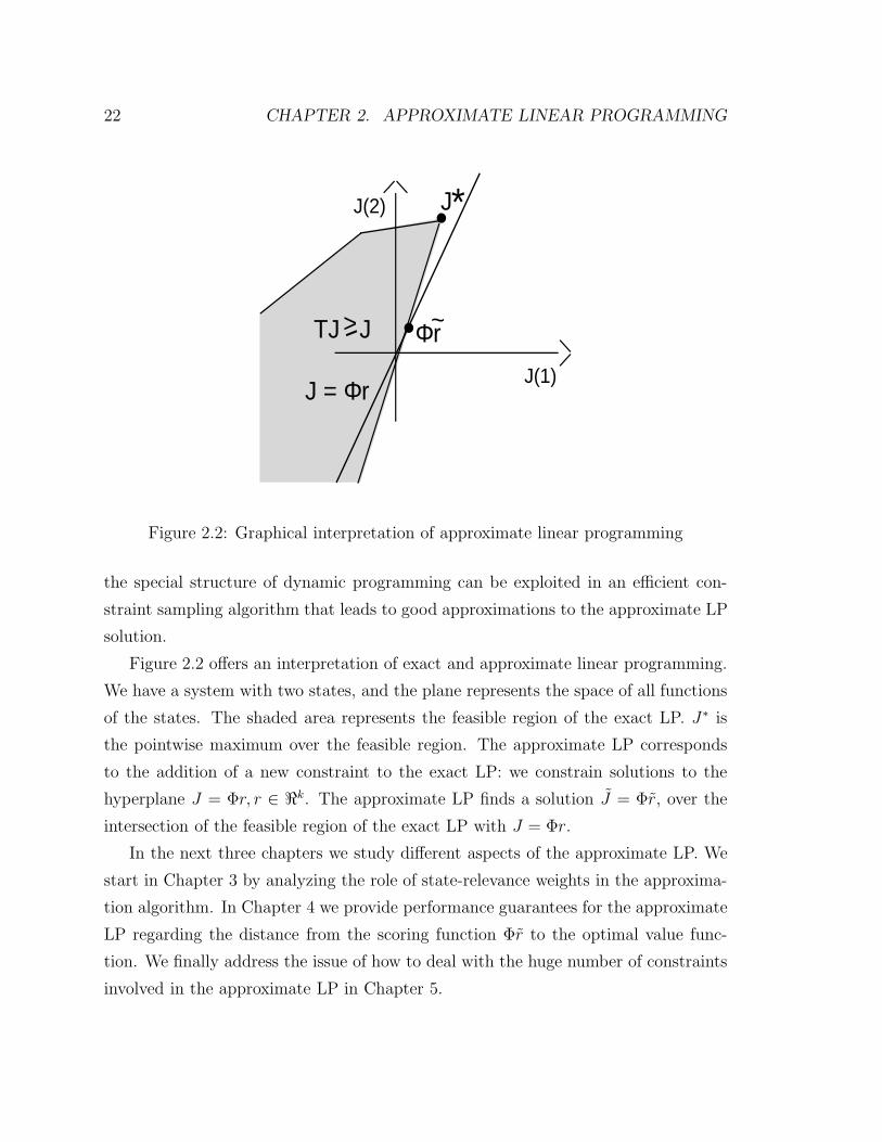
Figure 2.2: Graphical interpretation of approximate linear programming
the special structure of dynamic programming can be exploited in an efficient con-
straint sampling algorithm that leads to good approximations to the approximate LP
solution.
Figure 2.2 offers an interpretation of exact and approximate linear programming.
We have a system with two states, and the plane represents the space of all functions
of the states. The shaded area represents the feasible region of the exact LP. J∗ is
the pointwise maximum over the feasible region. The approximate LP corresponds
to the addition of a new constraint to the exact LP: we constrain solutions to the
hyperplane J = Φr, r ∈ <k. The approximate LP finds a solution J = Φr, over the
intersection of the feasible region of the exact LP with J = Φr.
In the next three chapters we study different aspects of the approximate LP. We
start in Chapter 3 by analyzing the role of state-relevance weights in the approxima-
tion algorithm. In Chapter 4 we provide performance guarantees for the approximate
LP regarding the distance from the scoring function Φr to the optimal value func-
tion. We finally address the issue of how to deal with the huge number of constraints
involved in the approximate LP in Chapter 5.
Chapter 3
State-Relevance Weights
Optimizing multiple objectives simultaneously imposes that certain tradeoffs must
be made: unless all objectives are completely aligned, there will be conflict and the
need to compromise on some of them. Approximating the optimal value function
over a large domain such as the state space poses the same problem. With only
limited approximation capacity, we cannot expect to obtain an approximation that is
uniformly good throughout the state space; in particular, the maximum error over all
states can become arbitrarily large as the problem dimensions increase. Therefore we
face the question of how to balance the accuracy of the approximation over different
portions of the state space. This chapter is dedicated to addressing this issue.
We first show how approximate linear programming provides the opportunity for
assigning different weights — state-relevance weights — to approximation errors over
different portions of the state space, therefore allowing for emphasis regions of greater
importance. We then develop a bound on the performance losses resulting from use
of a scoring function generated by approximate linear programming instead of the
optimal value function. We finally provide two examples motivating heuristics for
identifying what regions of the state space should be assigned higher state-relevance
weights.
23
24 CHAPTER 3. STATE-RELEVANCE WEIGHTS
3.1 State-Relevance Weights in the Approximate
LP
In the exact LP, for any vector c with positive components, maximizing cTJ yields
J∗. In other words, the choice of state-relevance weights does not influence the solu-
tion. The same statement does not hold for the approximate LP. In fact, as we will
demonstrate in this chapter, the choice of state-relevance weights bears a significant
impact on the quality of the resulting approximation.
To motivate the role of state-relevance weights, let us start with a lemma that
offers an interpretation of their function in the approximate LP. This lemma makes
use of a norm ‖ · ‖1,c, defined by
‖J‖1,c =∑x∈S
c(x)|J(x)|.
Lemma 3.1. A vector r solves
max cT Φr
s.t. TΦr ≥ Φr,
if and only if it solves
min ‖J∗ − Φr‖1,c
s.t. TΦr ≥ Φr.
Proof: It is well known that the dynamic programming operator T is monotonic.
From this and the fact that T is a contraction with fixed point J∗, it follows that, for
any J with J ≤ TJ , we have
J ≤ TJ ≤ T 2J ≤ ... ≤ J∗.
3.2. ON THE QUALITY OF POLICIES GENERATED BY ALP 25
Hence, any r that is a feasible solution to the optimization problems under consider-
ation satisfies Φr ≤ J∗. It follows that
‖J∗ − Φr‖1,c =∑x∈S
c(x)|J∗(x)− (Φr)(x)| = cTJ∗ − cT Φr,
and maximizing cT Φr is therefore equivalent to minimizing ‖J∗ − Φr‖1,c.
The preceding lemma points to an interpretation of the approximate LP as the
minimization of a certain weighted norm of the approximation error, with weights
equal to the state-relevance weights. This suggests that c specifies the tradeoff in the
quality of the approximation across different states, and we can lead the algorithm to
generate better approximations in a region of the state space by assigning relatively
larger weight to that region. In the next sections, we identify states that should be
weighted heavily to improve performance of the policy generated by the approximate
LP.
3.2 On The Quality of Policies Generated by ALP
In deriving a scoring function as a substitute to the optimal value function, a central
question is how to compare different scoring functions. A possible measure of quality
is the distance to the optimal value function; intuitively, we expect that the better
the scoring function captures the real long-run advantage of being in a given state,
the better the policy it generates. A more direct measure is a comparison between the
actual costs incurred by using the greedy policy associated with the scoring function
and those incurred by an optimal policy. In this section, we provide a bound on the
cost increase incurred by using scoring functions generated by approximated linear
programming.
Recall that we are interested in minimizing discounted costs over infinite horizon.
Complete information about the costs associated with a policy u is provided the func-
tion Ju (2.1), which provides the expected infinite-horizon discounted cost incurred
by using policy u as a function of the initial state in the system.
Comparing costs associated with two different policies requires comparison of two
26 CHAPTER 3. STATE-RELEVANCE WEIGHTS
functions on the state space. In turn, comparison of functions involves choice of a
metric defined on the space of these functions. We consider as a measure of the
quality of policy u the expected increase in the infinite-horizon discounted cost, con-
ditioned on the initial state of the system being distributed according to a probability
distribution ν; i.e.,
EX∼ν [Ju(X)− J∗(X)] = ‖Ju − J∗‖1,ν .
It will be useful to define a measure µu,ν over the state space associated with each
policy u and probability distribution ν, given by
µTu,ν = (1− α)νT
∞∑t=0
αtP tu. (3.1)
Note that, since∑∞
t=0 αtP t
u = (I − αPu)−1, we also have
µTu,ν = (1− α)νT (I − αPu)
−1.
The measure µu,ν captures the expected frequency of visits to each state when
the system runs under policy u, conditioned on the initial state being distributed
according to ν. Future visits are discounted according to the discount factor α.
Lemma 3.2. µu,ν is a probability distribution.
Proof: Let e be the vector of all ones. Then we have
∑x∈S
µu,ν(x) = (1− α)νT∞∑
t=0
αtP tue
= (1− α)νT∞∑
t=0
αte
= (1− α)νT (1− α)−1e
= 1,
and the claim follows.
3.2. ON THE QUALITY OF POLICIES GENERATED BY ALP 27
We are now poised to prove the following bound on the expected cost increase
associated with policies generated by approximate linear programming.
Theorem 3.1. Let J : S 7→ < be such that TJ ≥ J . Then
‖JuJ− J∗‖1,ν ≤ 1
1− α‖J − J∗‖1,µuJ,ν . (3.2)
Proof: We have
‖JuJ− J‖1,µuJ ,ν ≤ ‖JuJ
− TuJJ‖1,µuJ ,ν + ‖TuJ
J − J‖1,µuJ ,ν
= ‖TuJJuJ
− TuJJ‖1,µuJ ,ν + ‖TuJ
J − J‖1,µuJ ,ν
= α‖Pu(JuJ− J)‖1,µuJ,ν + ‖TuJ
J − J‖1,µuJ ,ν . (3.3)
where we first applied the triangle inequality and then JuJ= TuJ
JuJ.
By Corollary 2.1, since J ≤ TJ , we have J ≤ J∗ ≤ JuJ. It follows that
‖Pu(JuJ− J)‖1,µuJ,ν = µT
uJ ,νPu(JuJ− J). (3.4)
Combining (3.3) and (3.4), we get
‖JuJ− J‖1,µuJ ,ν ≤ αµT
uJ ,νPu(JuJ− J) + ‖TuJ
J − J‖1,µuJ ,ν
µTuJ ,ν(JuJ
− J) ≤ αµTuJ ,νPu(JuJ
− J) + ‖TuJJ − J‖1,µuJ ,ν
µTuJ ,ν(I − αPu)(JuJ
− J) ≤ ‖TuJJ − J‖1,µuJ,ν
(1− α)νT (I − αPu)−1(I − αPu)(JuJ
− J) ≤ ‖TuJJ − J‖1,µuJ,ν
(1− α)νT (JuJ− J) ≤ ‖TuJ
J − J‖1,µuJ,ν
(1− α)‖JuJ− J‖1,ν ≤ ‖TuJ
J − J‖1,µuJ,ν . (3.5)
Finally, we have J ≤ TJ = TuJJ ≤ J∗, so that
‖TuJJ − J‖1,µuJ ,ν ≤ ‖J∗ − J‖1,µuJ,ν , (3.6)
28 CHAPTER 3. STATE-RELEVANCE WEIGHTS
and
‖JuJ− J∗‖1,ν ≤ ‖JuJ
− J‖1,ν . (3.7)
Combining (3.5), (3.6) and (3.7), we get
‖JuJ− J∗‖1,ν ≤ ‖JuJ
− J‖1,ν
≤ 1
1− α‖TuJ
J − J‖1,µuJ ,ν
≤ 1
1− α‖J∗ − J‖1,µuJ ,ν ,
and the claim follows.
Theorem 3.1 has some interesting implications. Recall from Lemma 3.1 that the
approximate LP generates a scoring function Φr minimizing ‖Φr − J∗‖1,c over the
feasible region; contrasting this result with the bound on the increase in costs (3.2),
we might want to choose state-relevance weights c that capture the (discounted)
frequency with which different states are expected to be visited. The theorem also
sheds light on how beliefs about the initial state of the system can be factored into
the approximate LP.
Note that the frequency with which different states are visited in general depends
on the policy being used. One possibility is to have an iterative scheme, where
the approximate LP is solved multiple times with state-relevance weights adjusted
according to the intermediate policies being generated. The next section explores a
different approach geared towards problems exhibiting special structure.
3.3 Heuristic Choices of State-Relevance Weights
Theorem 3.1 suggests the use of state-relevance weights that emphasize states visited
often by reasonable policies. A plausible conjecture is that some problems will exhibit
structure making it relatively easy to take guesses about which states are desirable
and therefore more likely to be visited often by reasonable policies, and which ones
are typically avoided and rarely visited. We present two examples illustrating these
ideas.
3.3. HEURISTIC CHOICES OF STATE-RELEVANCE WEIGHTS 29
1
g(1) g(2) g(3)
2 3
1−δ,δ
δ,1−δ
δ
1−2δ 1−δ
δ
δ
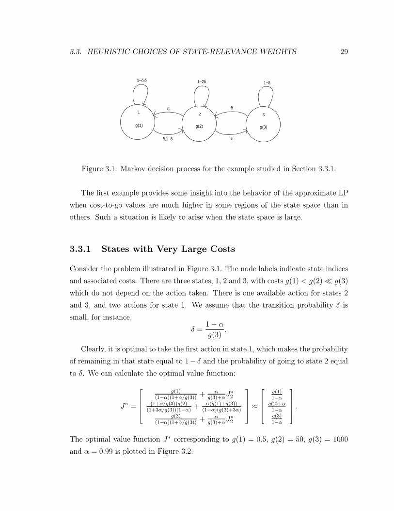
Figure 3.1: Markov decision process for the example studied in Section 3.3.1.
The first example provides some insight into the behavior of the approximate LP
when cost-to-go values are much higher in some regions of the state space than in
others. Such a situation is likely to arise when the state space is large.
3.3.1 States with Very Large Costs
Consider the problem illustrated in Figure 3.1. The node labels indicate state indices
and associated costs. There are three states, 1, 2 and 3, with costs g(1) < g(2) � g(3)
which do not depend on the action taken. There is one available action for states 2
and 3, and two actions for state 1. We assume that the transition probability δ is
small, for instance,
δ =1− α
g(3).
Clearly, it is optimal to take the first action in state 1, which makes the probability
of remaining in that state equal to 1− δ and the probability of going to state 2 equal
to δ. We can calculate the optimal value function:
J∗ =
g(1)(1−α)(1+α/g(3))
+ αg(3)+α
J∗2(1+α/g(3))g(2)
(1+3α/g(3))(1−α)+ α(g(1)+g(3))
(1−α)(g(3)+3α)g(3)
(1−α)(1+α/g(3))+ α
g(3)+αJ∗2
≈
g(1)1−α
g(2)+α1−αg(3)1−α
.
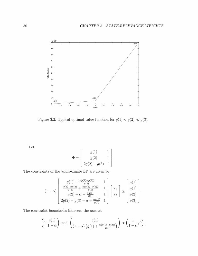
The optimal value function J∗ corresponding to g(1) = 0.5, g(2) = 50, g(3) = 1000
and α = 0.99 is plotted in Figure 3.2.
30 CHAPTER 3. STATE-RELEVANCE WEIGHTS
1 1.2 1.4 1.6 1.8 2 2.2 2.4 2.6 2.8 30
1
2
3
4
5
6
7
8
9
10x 10
4
state
valu
e fu
nctio
n
J(1)
J(2)
J(3)
Figure 3.2: Typical optimal value function for g(1) < g(2) � g(3).
Let
Φ =
g(1) 1
g(2) 1
2g(2)− g(3) 1
.
The constraints of the approximate LP are given by
(1− α)
g(1) + α(g(1)−g(2))g(3)
1g(1)−αg(2)
1−α+ α(g(2)−g(1))
g(3)1
g(2) + α− αg(1)g(3)
1
2g(2)− g(3)− α + αg(2)g(3)
1
r1
r2
≤
g(1)
g(1)
g(2)
g(3)
.
The constraint boundaries intersect the axes at
(0,
g(1)
1− α
)and
g(1)
(1− α)(g(1) + α(g(1)−g(2))
g(3)
) ≈ (
1
1− α, 0)
;
3.3. HEURISTIC CHOICES OF STATE-RELEVANCE WEIGHTS 31
(0,
g(1)
1− α
)and
g(1)
g(1)− αg(2) + (1− α)α(g(2)−g(1))g(3)
, 0
≈ (−ε, 0);
(0,
g(2)
1− α
)and
1
(1− α)(1 + α
g(2)− αg(1)
g(2)g(3)
) , 0 ≈ (
1− ε
1− α, 0)
;
(0,
g(3)
1− α
)and
g(3)
(1− α)(2g(2)− g(3)− α + αg(2)
g(3)
) , 0 ≈ (−M, 0),
where ε represents a relatively small positive number and M represents a relatively
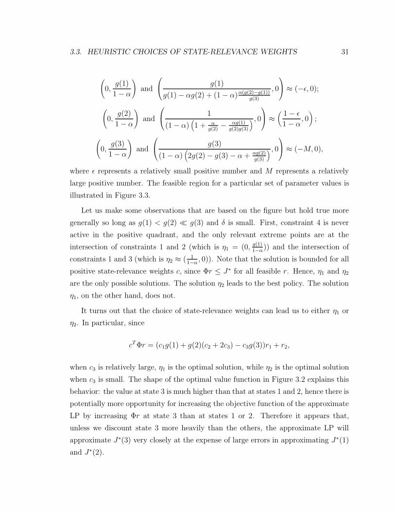
large positive number. The feasible region for a particular set of parameter values is
illustrated in Figure 3.3.
Let us make some observations that are based on the figure but hold true more
generally so long as g(1) < g(2) � g(3) and δ is small. First, constraint 4 is never
active in the positive quadrant, and the only relevant extreme points are at the
intersection of constraints 1 and 2 (which is η1 = (0, g(1)1−α
)) and the intersection of
constraints 1 and 3 (which is η2 ≈ ( 11−α
, 0)). Note that the solution is bounded for all
positive state-relevance weights c, since Φr ≤ J∗ for all feasible r. Hence, η1 and η2
are the only possible solutions. The solution η2 leads to the best policy. The solution
η1, on the other hand, does not.
It turns out that the choice of state-relevance weights can lead us to either η1 or
η2. In particular, since
cT Φr = (c1g(1) + g(2)(c2 + 2c3)− c3g(3))r1 + r2,
when c3 is relatively large, η1 is the optimal solution, while η2 is the optimal solution
when c3 is small. The shape of the optimal value function in Figure 3.2 explains this
behavior: the value at state 3 is much higher than that at states 1 and 2, hence there is
potentially more opportunity for increasing the objective function of the approximate
LP by increasing Φr at state 3 than at states 1 or 2. Therefore it appears that,
unless we discount state 3 more heavily than the others, the approximate LP will
approximate J∗(3) very closely at the expense of large errors in approximating J∗(1)
and J∗(2).
32 CHAPTER 3. STATE-RELEVANCE WEIGHTS
0 10 20 30 40 50 60150
100
50
0
50
100
150
feasible region
constraint 1
constraint 2
constraint 3
constraint 4
η
η
r
r
2
11
2
Figure 3.3: Typical feasible region for g(1) < g(2) << g(3). The arrow representscT Φ for a state-relevance weight c which yields a ”good” solution for the approximateLP.
3.3.2 Weights Induced by Steady-State Probabilities
The preceding example illustrates how the approximate LP is likely to yield poor
approximations for states with relatively low value function unless these states are
emphasized by state-relevance weights. From the theoretical bound develop in Theo-
rem 3.1, we know that state-relevance weights should also be chosen so as to emphasize
frequently visited states. The next example illustrates how in some cases it may be
possible to identify regions of the state space that would be visited often if the system
were to be controlled by a “good” policy, and how reasonably good state-relevance
weights can be found in that case. We expect structures enabling this kind of pro-
cedure to be reasonably common in large-scale problems, in which desirable policies
often exhibit some form of “stability,” guiding the system to a limited region of the
state space and allowing only infrequent excursions from this region.
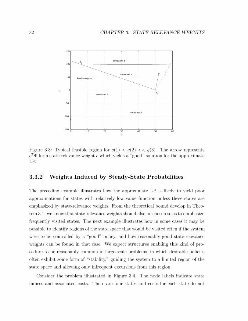
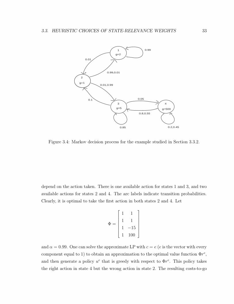
Consider the problem illustrated in Figure 3.4. The node labels indicate state
indices and associated costs. There are four states and costs for each state do not
3.3. HEURISTIC CHOICES OF STATE-RELEVANCE WEIGHTS 33
0.991
g=2
2
g=1
3
g=5
4
g=500
0.01
0.99,0.01
0.01,0.99
0.1
0.85
0.05
0.8,0.55
0.2,0.45
Figure 3.4: Markov decision process for the example studied in Section 3.3.2.
depend on the action taken. There is one available action for states 1 and 3, and two
available actions for states 2 and 4. The arc labels indicate transition probabilities.
Clearly, it is optimal to take the first action in both states 2 and 4. Let
Φ =
1 1
1 1
1 −15
1 100
and α = 0.99. One can solve the approximate LP with c = e (e is the vector with every
component equal to 1) to obtain an approximation to the optimal value function Φre,
and then generate a policy ue that is greedy with respect to Φre. This policy takes
the right action in state 4 but the wrong action in state 2. The resulting costs-to-go
34 CHAPTER 3. STATE-RELEVANCE WEIGHTS
are given by
Jue =
1560.9
2935.5
2978.3
3565.6
.
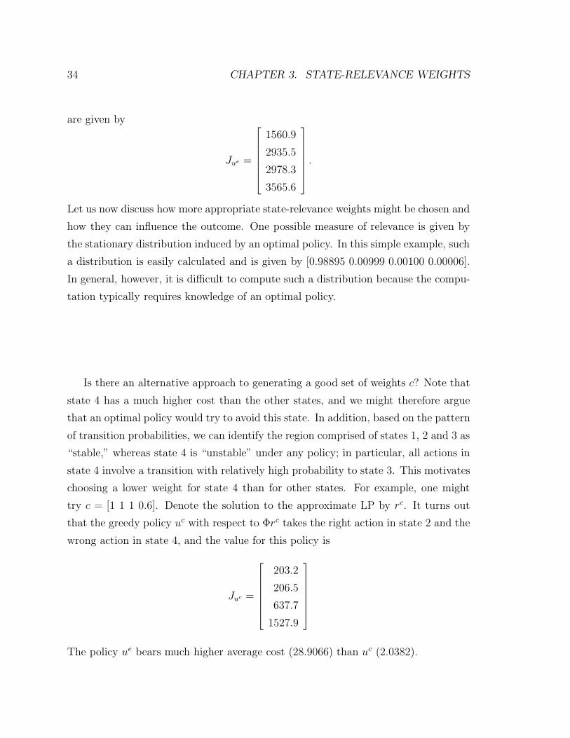
Let us now discuss how more appropriate state-relevance weights might be chosen and
how they can influence the outcome. One possible measure of relevance is given by
the stationary distribution induced by an optimal policy. In this simple example, such
a distribution is easily calculated and is given by [0.98895 0.00999 0.00100 0.00006].
In general, however, it is difficult to compute such a distribution because the compu-
tation typically requires knowledge of an optimal policy.
Is there an alternative approach to generating a good set of weights c? Note that
state 4 has a much higher cost than the other states, and we might therefore argue
that an optimal policy would try to avoid this state. In addition, based on the pattern
of transition probabilities, we can identify the region comprised of states 1, 2 and 3 as
“stable,” whereas state 4 is “unstable” under any policy; in particular, all actions in
state 4 involve a transition with relatively high probability to state 3. This motivates
choosing a lower weight for state 4 than for other states. For example, one might
try c = [1 1 1 0.6]. Denote the solution to the approximate LP by rc. It turns out
that the greedy policy uc with respect to Φrc takes the right action in state 2 and the
wrong action in state 4, and the value for this policy is
Juc =
203.2
206.5
637.7
1527.9
The policy ue bears much higher average cost (28.9066) than uc (2.0382).
3.4. CLOSING REMARKS 35
3.4 Closing Remarks
We have seen that the state-relevance weights can influence the quality of an approx-
imation. It is not clear how to find good weights in an efficient manner for larger
problems. However, our theoretical results and examples do motivate certain heuris-
tics for selecting weights. Theorem 3.1 suggests the use of an iterative scheme for
selection of state-relevance weights, with solution of multiple approximate LP’s and
weights being designed based on intermediate policies being generated. The examples
also suggest that given certain problem structures, certain portions of the state space
should be emphasized. First, it seems important to assign low weights to states with
high costs, as suggested by Example 3.3.1. Second, if the system when operated by
a good policy spends most of its time in a certain subset of the state space, it seems
that this subset should be weighted heavily, as suggested by Theorem 3.1 and illus-
trated by Example 3.3.2. We expect that these heuristics will not generally conflict.
In particular, in realistic large-scale problems, states with high costs should avoided,
and the system should spend most of its time in a low-cost region of the state space.

36 CHAPTER 3. STATE-RELEVANCE WEIGHTS
Chapter 4
Approximation Error Analysis
It is clear that a scoring function can only be as good as the approximation archi-
tecture that defines its representation. Historically, it has been difficult to show the
reverse: even if the approximation architecture includes good approximations to the
optimal value function, it usually remains uncertain whether approximate dynamic
programming algorithms are guaranteed to deliver a reasonable scoring function.
When the optimal value function lies within the span of the basis functions, the
approximate LP yields the optimal value function. Unfortunately, it is difficult in
practice to select a set of basis functions that contains the optimal value function
within its span. Instead, basis functions must be based on heuristics and simplified
analysis. One can only hope that the span comes close to the desired value function.
For the approximate LP to be useful, it should deliver good approximations when
the optimal value function is near the span of selected basis functions. In this chapter,
we develop bounds that ensure desirable results of this kind. We begin in Section 4.2
with a simple bound capturing the fact that, if the vector of all ones is in the span of
the basis functions, the error in the result of the approximate LP is proportional to
the minimal error given the selected basis functions. Though this result is interesting
in its own right, the bound is very loose — perhaps too much so to be useful in
practical contexts. In Section 4.3, however, we remedy this situation by providing a
tighter bound, which constitutes the main result in this chapter.
37
38 CHAPTER 4. APPROXIMATION ERROR ANALYSIS
J*
J = Φr
Φr~
Φr*
J(1)
J(2)
TJ J>
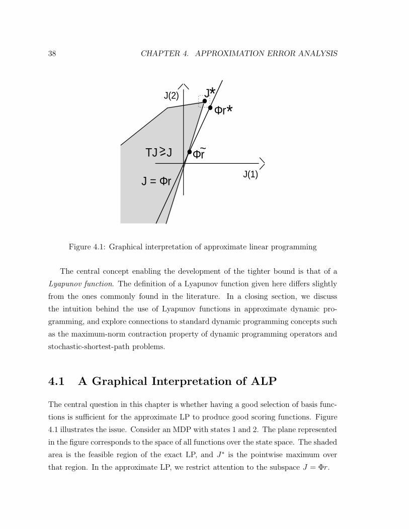
Figure 4.1: Graphical interpretation of approximate linear programming
The central concept enabling the development of the tighter bound is that of a
Lyapunov function. The definition of a Lyapunov function given here differs slightly
from the ones commonly found in the literature. In a closing section, we discuss
the intuition behind the use of Lyapunov functions in approximate dynamic pro-
gramming, and explore connections to standard dynamic programming concepts such
as the maximum-norm contraction property of dynamic programming operators and
stochastic-shortest-path problems.
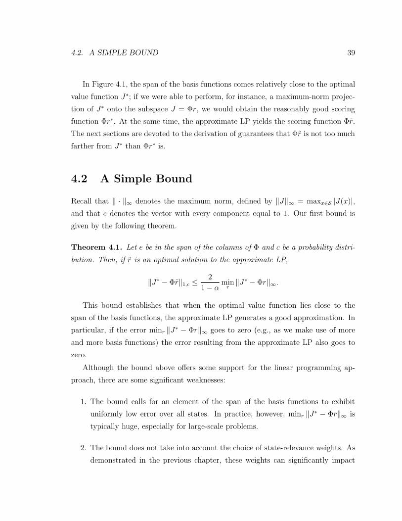
4.1 A Graphical Interpretation of ALP
The central question in this chapter is whether having a good selection of basis func-
tions is sufficient for the approximate LP to produce good scoring functions. Figure
4.1 illustrates the issue. Consider an MDP with states 1 and 2. The plane represented
in the figure corresponds to the space of all functions over the state space. The shaded
area is the feasible region of the exact LP, and J∗ is the pointwise maximum over
that region. In the approximate LP, we restrict attention to the subspace J = Φr.
4.2. A SIMPLE BOUND 39
In Figure 4.1, the span of the basis functions comes relatively close to the optimal
value function J∗; if we were able to perform, for instance, a maximum-norm projec-
tion of J∗ onto the subspace J = Φr, we would obtain the reasonably good scoring
function Φr∗. At the same time, the approximate LP yields the scoring function Φr.
The next sections are devoted to the derivation of guarantees that Φr is not too much
farther from J∗ than Φr∗ is.
4.2 A Simple Bound
Recall that ‖ · ‖∞ denotes the maximum norm, defined by ‖J‖∞ = maxx∈S |J(x)|,and that e denotes the vector with every component equal to 1. Our first bound is
given by the following theorem.
Theorem 4.1. Let e be in the span of the columns of Φ and c be a probability distri-
bution. Then, if r is an optimal solution to the approximate LP,
‖J∗ − Φr‖1,c ≤ 2
1− αmin
r‖J∗ − Φr‖∞.
This bound establishes that when the optimal value function lies close to the
span of the basis functions, the approximate LP generates a good approximation. In
particular, if the error minr ‖J∗ − Φr‖∞ goes to zero (e.g., as we make use of more
and more basis functions) the error resulting from the approximate LP also goes to
zero.
Although the bound above offers some support for the linear programming ap-
proach, there are some significant weaknesses:
1. The bound calls for an element of the span of the basis functions to exhibit
uniformly low error over all states. In practice, however, minr ‖J∗ − Φr‖∞ is
typically huge, especially for large-scale problems.
2. The bound does not take into account the choice of state-relevance weights. As
demonstrated in the previous chapter, these weights can significantly impact
40 CHAPTER 4. APPROXIMATION ERROR ANALYSIS
the quality of the scoring function. A meaningful bound should take them into
account.
In Section 4.3, we will state and prove the main result of this chapter, which provides
an improved bound that aims to alleviate the shortcomings listed above. First, we
prove Theorem 4.1.
Proof of Theorem 4.1
Let r∗ be one of the vectors minimizing ‖J∗ − Φr‖∞ and define ε = ‖J∗ − Φr∗‖∞.
The first step is to find a feasible point r such that Φr is within distance O(ε) of J∗.
Since
‖TΦr∗ − J∗‖∞ ≤ α‖Φr∗ − J∗‖∞,
we have
TΦr∗ ≥ J∗ − αεe. (4.1)
We also recall that for any vector J and any scalar k,
T (J − ke) = minu{gu + αPu(J − ke)}
= minu{gu + αPuJ − αke}
= minu{gu + αPuJ} − αke
= TJ − αke. (4.2)
Combining (4.1) and (4.2), we have
T (Φr∗ − ke) = TΦr∗ − αke
≥ J∗ − αεe− αke
≥ Φr∗ − (1 + α)εe− αke
= Φr∗ − ke+ [(1− α)k − (1 + α)ε] e.
4.3. AN IMPROVED BOUND 41
Since e is within the span of the columns of Φ, there exists a vector r such that
Φr = Φr∗ − (1 + α)ε
1− αe,
and r is a feasible solution to the approximate LP. By the triangle inequality,
‖Φr − J∗‖∞ ≤ ‖J∗ − Φr∗‖∞ + ‖Φr∗ − Φr‖∞ ≤ ε(1 +
1 + α
1− α
)=
2ε
1− α.
If r is an optimal solution to the approximate LP, by Lemma 3.1, we have
‖J∗ − Φr‖1,c ≤ ‖J∗ − Φr‖1,c
≤ ‖J∗ − Φr‖∞≤ 2ε
1− α
where the second inequality holds because c is a probability distribution. The result
follows.
4.3 An Improved Bound
To set the stage for the development of an improved bound, let us establish some
notation. First, we introduce a weighted maximum norm, defined by
‖J‖∞,γ = maxx∈S
γ(x)|J(x)|, (4.3)
for any γ : S 7→ <+. As opposed to the maximum norm employed in Theorem 4.1,
this norm allows for uneven weighting of errors across the state space.
We also introduce an operator H , defined by
(HV )(x) = maxa∈Ax
∑y∈S
Pa(x, y)V (y),
for all V : S 7→ <. For any V , (HV )(x) represents the maximum expected value of
V (Y ) if the current state is x and Y is a random variable representing the next state.
42 CHAPTER 4. APPROXIMATION ERROR ANALYSIS
For each V : S 7→ <, we define a scalar βV given by
βV = maxx
α(HV )(x)
V (x). (4.4)
We can now introduce the notion of a “Lyapunov function,” as follows.
Definition 4.1 (Lyapunov function) We call V : S 7→ <+ a Lyapunov function if
βV < 1.
Our definition of a Lyapunov function translates into the condition that there
exist V > 0 and β < 1 such that
α(HV )(x) ≤ βV (x), ∀x ∈ S. (4.5)
If α were equal to 1, this would look like a Lyapunov stability condition: the maximum
expected value (HV )(x) at the next time step must be less than the current value
V (x). In general, α is less than 1, and this introduces some slack in the condition.
Our error bound for the approximate LP will grow proportionately with 1/(1−βV ),
and we therefore want βV to be small. Note that βV becomes smaller as the (HV )(x)’s
become small relative to the V (x)’s; βV conveys a degree of “stability,” with smaller
values representing stronger stability. Therefore our bound suggests that, the more
stable the system is, the easier it may be for the approximate LP to generate a good
scoring function.
We are now ready to state our main result. For any given function V mapping Sto positive reals, we use 1/V as shorthand for a function x 7→ 1/V (x).
Theorem 4.2. Let r be a solution of the approximate LP. Then, for any v ∈ <K
such that Φv is a Lyapunov function,
‖J∗ − Φr‖1,c ≤ 2cT Φv
1− βΦvmin
r‖J∗ − Φr‖∞,1/Φv. (4.6)
Let us now discuss how this new theorem addresses the shortcomings of The-
orem 4.1 listed in the previous section. We treat in turn the two items from the
aforementioned list.
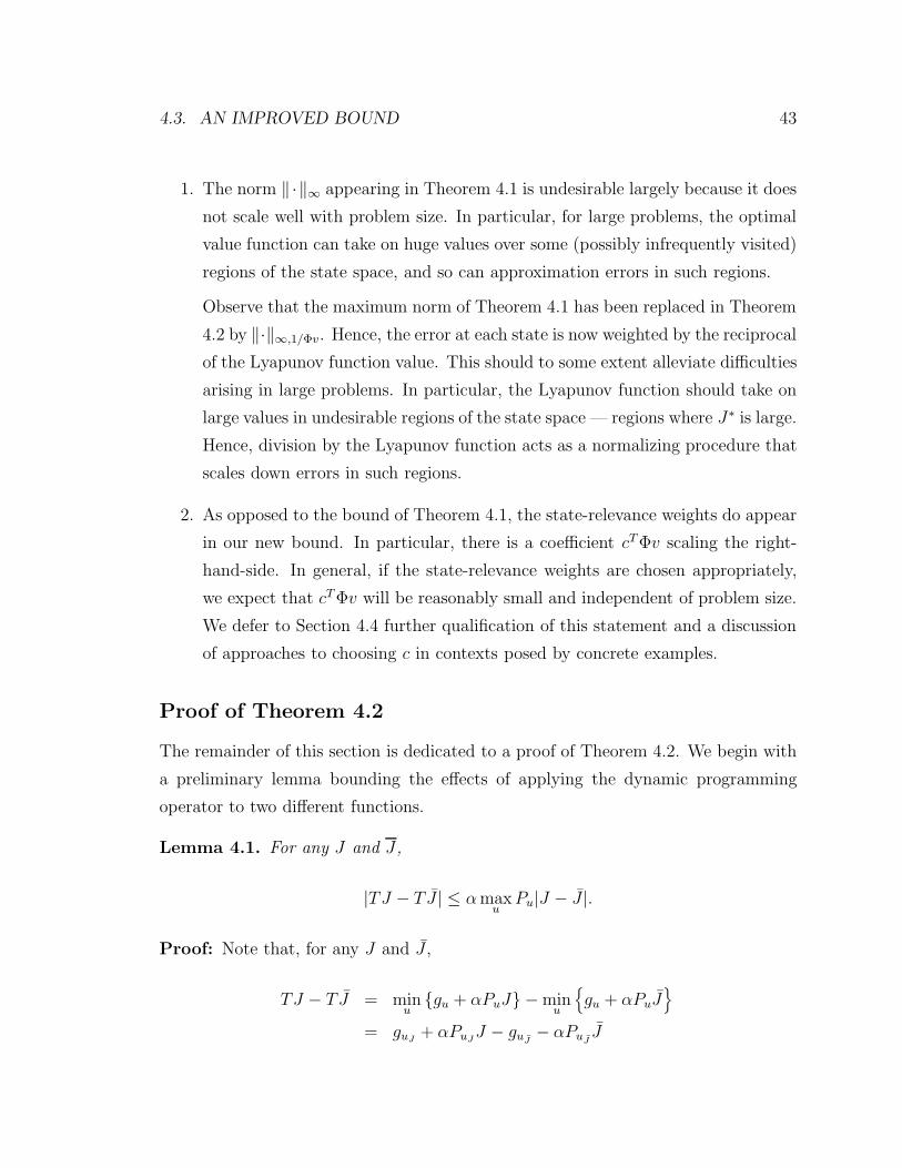
4.3. AN IMPROVED BOUND 43
1. The norm ‖·‖∞ appearing in Theorem 4.1 is undesirable largely because it does
not scale well with problem size. In particular, for large problems, the optimal
value function can take on huge values over some (possibly infrequently visited)
regions of the state space, and so can approximation errors in such regions.
Observe that the maximum norm of Theorem 4.1 has been replaced in Theorem
4.2 by ‖·‖∞,1/Φv. Hence, the error at each state is now weighted by the reciprocal
of the Lyapunov function value. This should to some extent alleviate difficulties
arising in large problems. In particular, the Lyapunov function should take on
large values in undesirable regions of the state space — regions where J∗ is large.
Hence, division by the Lyapunov function acts as a normalizing procedure that
scales down errors in such regions.
2. As opposed to the bound of Theorem 4.1, the state-relevance weights do appear
in our new bound. In particular, there is a coefficient cT Φv scaling the right-
hand-side. In general, if the state-relevance weights are chosen appropriately,
we expect that cT Φv will be reasonably small and independent of problem size.
We defer to Section 4.4 further qualification of this statement and a discussion
of approaches to choosing c in contexts posed by concrete examples.
Proof of Theorem 4.2
The remainder of this section is dedicated to a proof of Theorem 4.2. We begin with
a preliminary lemma bounding the effects of applying the dynamic programming
operator to two different functions.
Lemma 4.1. For any J and J ,
|TJ − T J | ≤ αmaxu
Pu|J − J |.
Proof: Note that, for any J and J ,
TJ − T J = minu{gu + αPuJ} −min
u
{gu + αPuJ
}= guJ
+ αPuJJ − guJ
− αPuJJ

44 CHAPTER 4. APPROXIMATION ERROR ANALYSIS
≤ guJ+ αPuJ
J − guJ− αPuJ
J
≤ αmaxu
Pu(J − J)
≤ αmaxu
Pu|J − J |,
where uJ and uJ denote greedy policies with respect to J and J , respectively. An
entirely analogous argument gives us
T J − TJ ≤ αmaxu
Pu|J − J |,
and the result follows.
Based on the above lemma, we can place the following bound on constraint vio-
lations in the approximate LP.
Lemma 4.2. For any vector V with positive components and any vector J ,
TJ ≥ J − (αHV + V ) ‖J∗ − J‖∞,1/V . (4.7)
Proof: Note that
|J∗(x)− J(x)| ≤ ‖J∗ − J‖∞,1/V V (x).
By Lemma 4.1,
|(TJ∗)(x)− (TJ)(x)| ≤ αmaxa
∑y∈S
Pa(x, y)|J∗(y)− J(y)|
≤ α‖J∗ − J‖∞,1/V maxa∈Ax
∑y∈S
Pa(x, y)V (y)
= α‖J∗ − J‖∞,1/V (HV )(x).
Letting ε = ‖J∗ − J‖∞,1/V , it follows that
(TJ)(x) ≥ J∗(x)− αε(HV )(x)
≥ J(x)− εV (x)− αε(HV )(x).
The result follows.
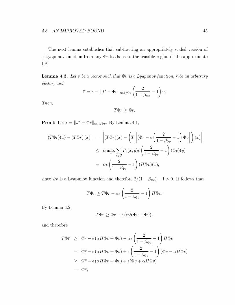
4.3. AN IMPROVED BOUND 45
The next lemma establishes that subtracting an appropriately scaled version of
a Lyapunov function from any Φr leads us to the feasible region of the approximate
LP.
Lemma 4.3. Let v be a vector such that Φv is a Lyapunov function, r be an arbitrary
vector, and
r = r − ‖J∗ − Φr‖∞,1/Φv
(2
1− βΦv− 1
)v.
Then,
TΦr ≥ Φr.
Proof: Let ε = ‖J∗ − Φr‖∞,1/Φv. By Lemma 4.1,
|(TΦr)(x)− (TΦr) (x)| =
∣∣∣∣∣(TΦr)(x)−(T
[(Φr − ε
(2
1− βΦv− 1
)Φv
])(x)
∣∣∣∣∣≤ αmax
a
∑y∈S
Pa(x, y)ε
(2
1− βΦv− 1
)(Φv)(y)
= αε
(2
1− βΦv
− 1
)(HΦv)(x),
since Φv is a Lyapunov function and therefore 2/(1− βΦv)− 1 > 0. It follows that
TΦr ≥ TΦr − αε
(2
1− βΦv− 1
)HΦv.
By Lemma 4.2,
TΦr ≥ Φr − ε (αHΦv + Φv) ,
and therefore
TΦr ≥ Φr − ε (αHΦv + Φv)− αε
(2
1− βΦv
− 1
)HΦv
= Φr − ε (αHΦv + Φv) + ε
(2
1− βΦv− 1
)(Φv − αHΦv)
≥ Φr − ε (αHΦv + Φv) + ε(Φv + αHΦv)
= Φr,

46 CHAPTER 4. APPROXIMATION ERROR ANALYSIS
where the last inequality follows from the fact that Φv − αHΦv > 0 and
2
1− βΦv
− 1 =2
1−maxxα(HΦv)(x)
(Φv)(x)
− 1
= maxx
2(Φv)(x)
(Φv)(x)− α(HΦv)(x)− 1
= maxx
(Φv)(x) + α(HΦv)(x)
(Φv)(x)− α(HΦv)(x).
Proof of Theorem 4.2: Given the preceding lemmas, we are poised to prove Theo-
rem 4.2. From Lemma 4.3, we know that r = r∗ − ‖J∗ − Φr∗‖∞,1/Φv
(2
1−βΦv− 1
)v is
a feasible solution for the approximate LP. It follows that
‖Φr − Φr∗‖∞,1/Φv ≤ ‖J∗ − Φr∗‖∞,1/Φv
(2
1− βΦv− 1
)‖Φv‖∞,1/Φv
= ‖J∗ − Φr∗‖∞,1/Φv
(2
1− βΦv− 1
).
From Lemma 3.1, we have
‖J∗ − Φr‖1,c ≤ ‖J∗ − Φr‖1,c
=∑x
c(x)(Φv)(x)|J∗(x)− (Φr)(x)|
(Φv)(x)
≤(∑
x
c(x)(Φv)(x)
)max
x
|J∗(x)− (Φr)(x)|(Φv)(x)
= cT Φv‖J∗ − Φr‖∞,1/Φv
≤ cT Φv(‖J∗ − Φr∗‖∞,1/Φv + ‖Φr − Φr∗‖∞,1/Φv
)
≤ cT Φv
(‖J∗ − Φr∗‖∞,1/Φv + ‖J∗ − Φr∗‖∞,1/Φv
(2
1− βΦv
− 1
))
≤ 2
1− βΦvcT Φv‖J∗ − Φr∗‖∞,1/Φv.
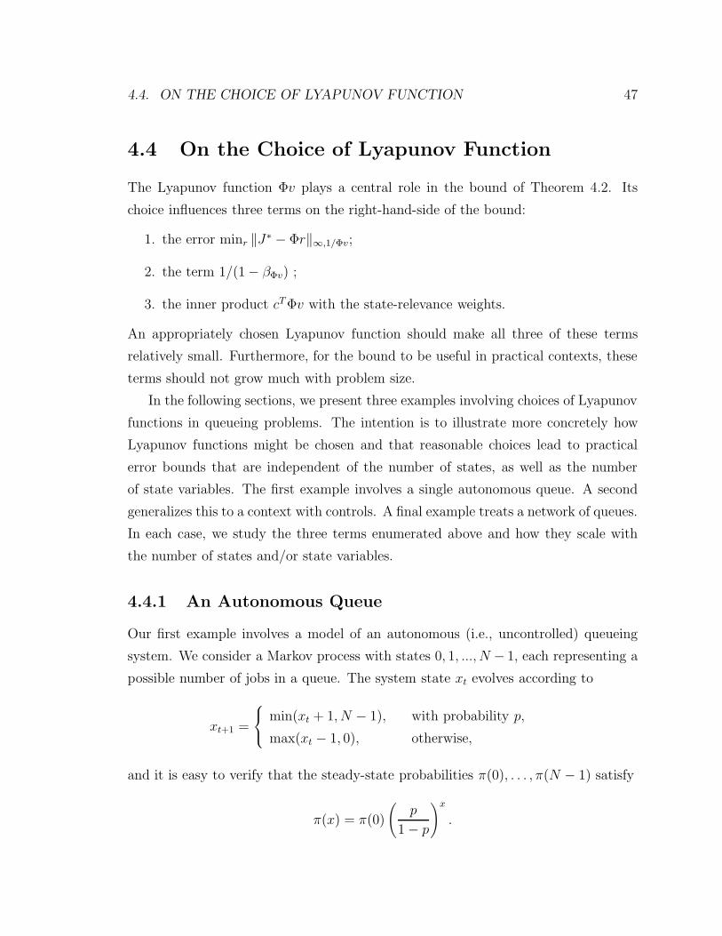
4.4. ON THE CHOICE OF LYAPUNOV FUNCTION 47
4.4 On the Choice of Lyapunov Function
The Lyapunov function Φv plays a central role in the bound of Theorem 4.2. Its
choice influences three terms on the right-hand-side of the bound:
1. the error minr ‖J∗ − Φr‖∞,1/Φv;
2. the term 1/(1− βΦv) ;
3. the inner product cT Φv with the state-relevance weights.
An appropriately chosen Lyapunov function should make all three of these terms
relatively small. Furthermore, for the bound to be useful in practical contexts, these
terms should not grow much with problem size.
In the following sections, we present three examples involving choices of Lyapunov
functions in queueing problems. The intention is to illustrate more concretely how
Lyapunov functions might be chosen and that reasonable choices lead to practical
error bounds that are independent of the number of states, as well as the number
of state variables. The first example involves a single autonomous queue. A second
generalizes this to a context with controls. A final example treats a network of queues.
In each case, we study the three terms enumerated above and how they scale with
the number of states and/or state variables.
4.4.1 An Autonomous Queue
Our first example involves a model of an autonomous (i.e., uncontrolled) queueing
system. We consider a Markov process with states 0, 1, ..., N − 1, each representing a
possible number of jobs in a queue. The system state xt evolves according to
xt+1 =
min(xt + 1, N − 1), with probability p,
max(xt − 1, 0), otherwise,
and it is easy to verify that the steady-state probabilities π(0), . . . , π(N − 1) satisfy
π(x) = π(0)
(p
1− p
)x
.
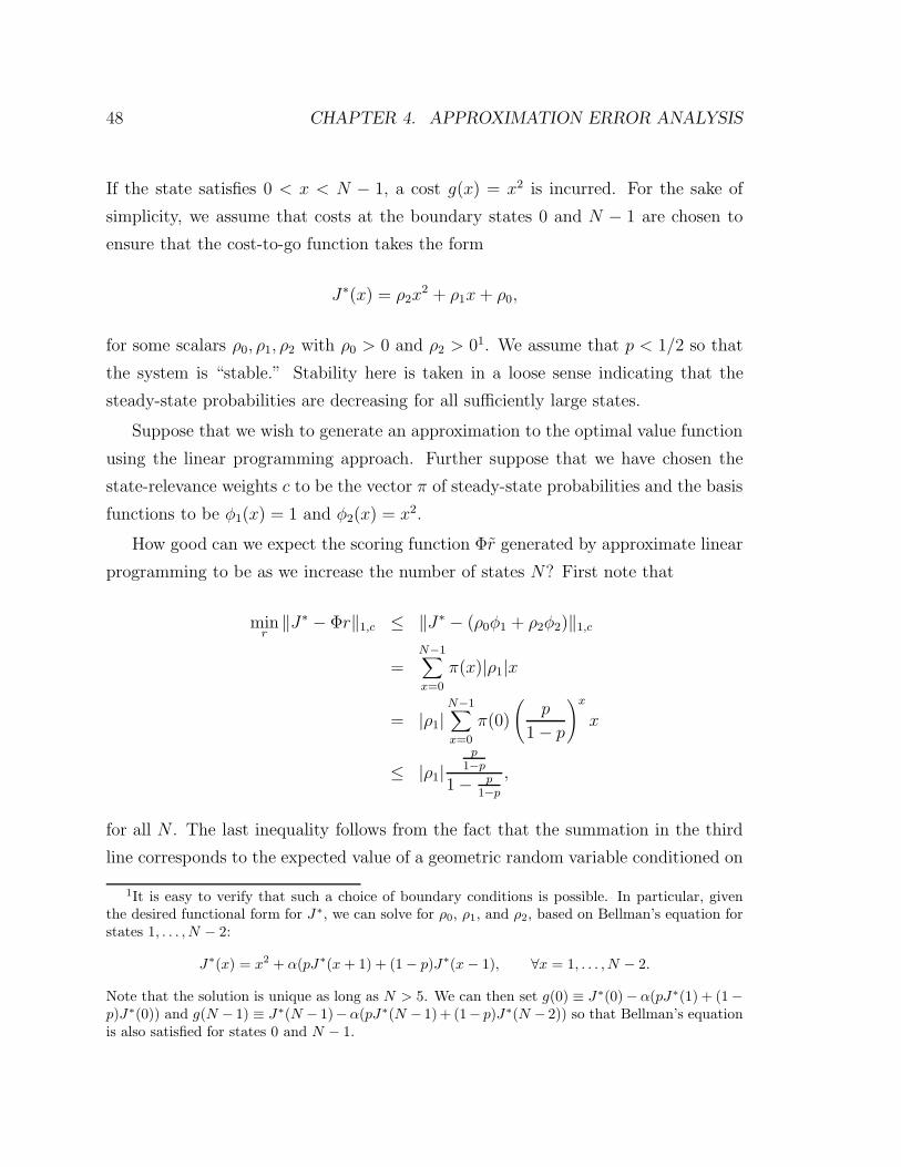
48 CHAPTER 4. APPROXIMATION ERROR ANALYSIS
If the state satisfies 0 < x < N − 1, a cost g(x) = x2 is incurred. For the sake of
simplicity, we assume that costs at the boundary states 0 and N − 1 are chosen to
ensure that the cost-to-go function takes the form
J∗(x) = ρ2x2 + ρ1x+ ρ0,
for some scalars ρ0, ρ1, ρ2 with ρ0 > 0 and ρ2 > 01. We assume that p < 1/2 so that
the system is “stable.” Stability here is taken in a loose sense indicating that the
steady-state probabilities are decreasing for all sufficiently large states.
Suppose that we wish to generate an approximation to the optimal value function
using the linear programming approach. Further suppose that we have chosen the
state-relevance weights c to be the vector π of steady-state probabilities and the basis
functions to be φ1(x) = 1 and φ2(x) = x2.
How good can we expect the scoring function Φr generated by approximate linear
programming to be as we increase the number of states N? First note that
minr‖J∗ − Φr‖1,c ≤ ‖J∗ − (ρ0φ1 + ρ2φ2)‖1,c
=N−1∑x=0
π(x)|ρ1|x
= |ρ1|N−1∑x=0
π(0)
(p
1− p
)x
x
≤ |ρ1|p
1−p
1− p1−p
,
for all N . The last inequality follows from the fact that the summation in the third
line corresponds to the expected value of a geometric random variable conditioned on
1It is easy to verify that such a choice of boundary conditions is possible. In particular, giventhe desired functional form for J∗, we can solve for ρ0, ρ1, and ρ2, based on Bellman’s equation forstates 1, . . . , N − 2:
J∗(x) = x2 + α(pJ∗(x + 1) + (1− p)J∗(x − 1), ∀x = 1, . . . , N − 2.
Note that the solution is unique as long as N > 5. We can then set g(0) ≡ J∗(0)− α(pJ∗(1) + (1−p)J∗(0)) and g(N − 1) ≡ J∗(N − 1)−α(pJ∗(N − 1)+ (1− p)J∗(N − 2)) so that Bellman’s equationis also satisfied for states 0 and N − 1.
4.4. ON THE CHOICE OF LYAPUNOV FUNCTION 49
its being less than N . Hence, minr ‖J∗ − Φr‖1,c is uniformly bounded over N . One
would hope that ‖J∗−Φr‖1,c, with r being an outcome of the approximate LP, would
be similarly uniformly bounded over N . It is clear that Theorem 4.1 does not offer a
uniform bound of this sort. In particular, the term minr ‖J∗−Φr‖∞ on the right-hand-
side grows proportionately with N and is unbounded as N increases. Fortunately,
this situation is remedied by Theorem 4.2, which does provide a uniform bound.
In particular, as we will show in the remainder of this section, for an appropriate
Lyapunov function V = Φv, the values of minr ‖J∗ − Φr‖∞,1/V , 1/(1 − βV ) and
cTV are all uniformly bounded over N , and together these values offer a bound on
‖J∗ − Φr‖1,c that is uniform over N .
We will make use of a Lyapunov function
V (x) = x2 +2
1− α,
which is clearly within the span of our basis functions φ1 and φ2. Given this choice,
we have
minr‖J∗ − Φr‖∞,1/V ≤ max
x≥0
|ρ2x2 + ρ1x+ ρ0 − ρ2x
2 − ρ0|x2 + 2/(1− α)
= maxx≥0
|ρ1|xx2 + 2/(1− α)
≤ |ρ1|2√
2/(1− α).
Hence, minr ‖J∗ − Φr‖∞,1/V is uniformly bounded over N .
We next show that 1/(1− βV ) is uniformly bounded over N . In order to do that,
we find bounds on HV in terms of V . For 0 < x < N − 1, we have
α(HV )(x) = α[p(x2 + 2x+ 1 +
2
1− α
)+ (1− p)
(x2 − 2x+ 1 +
2
1− α
)]
= α[x2 +
2
1− α+ 1 + 2x(2p− 1)
]
≤ α(x2 +
2
1− α+ 1
)
50 CHAPTER 4. APPROXIMATION ERROR ANALYSIS
= V (x)
(α +
α
V (x)
)
≤ V (x)
(α +
1
V (0)
)
= V (x)1 + α
2.
For x = 0, we have
α(HV )(0) = α[p(1 +
2
1− α
)+ (1− p)
2
1− α
]
= αp+ α2
1− α
≤ V (0)(α +
1− α
2
)
= V (0)1 + α
2.
Finally, we clearly have
α(HV )(N − 1) ≤ αV (N − 1) ≤ V (N − 1)1 + α
2,
since the only possible transitions from state N − 1 are to states x ≤ N − 1 and V
is a nondecreasing function. Therefore, βV ≤ (1 + α)/2 and 1/(1− βV ) is uniformly
bounded on N .
We now treat cTV . Note that for N ≥ 1,
cTV =N−1∑x=0
π(0)
(p
1− p
)x (x2 +
2
1− α
)
=1− p/(1− p)
1− [p/(1− p)]N
N−1∑x=0
(p
1− p
)x (x2 +
2
1− α
)
≤ 1− p/(1− p)
1− p/(1− p)
∞∑x=0
(p
1− p
)x (x2 +
2
1− α
)
=1− p
1− 2p
(2
1− α+ 2
p2
(1− 2p)2+
p
1− 2p
),
so cTV is uniformly bounded for all N .
4.4. ON THE CHOICE OF LYAPUNOV FUNCTION 51
4.4.2 A Controlled Queue
In the previous example, we treated the case of an autonomous queue and showed
how the terms involved in the error bound of Theorem 4.2 are uniformly bounded on
the number of states N . We now address a more general case in which we can control
the queue service rate. For any time t and state 0 < xt < N − 1, the next state is
given by
xt+1 =
xt − 1, with probability q(xt),
xt + 1, with probability p,
xt, otherwise.
From state 0, a transition to state 1 or 0 occurs with probabilities p or 1 − p, re-
spectively. From state N − 1, a transition to state N − 2 or N − 1 occurs with
probabilities q(N − 2) or 1− q(N − 2), respectively. The arrival probability p is the
same for all states and we assume that p < 1/2. The action to be chosen in each
state x is the departure probability or service rate q(x), which takes values in a fi-
nite set {qi, i = 1, ..., A}. We assume that qA = 1 − p > p, therefore the queue is
“stabilizable”. The cost incurred at state x if action q is taken is given by
g(x, q) = x2 +m(q),
where m is a nonnegative and increasing function.
As discussed before, our objective is to show that the terms involved in the error
bound of Theorem 4.2 are uniformly bounded over N . We start by finding a suit-
able Lyapunov function based on our knowledge of the problem structure. In the
autonomous case, the choice of the Lyapunov function was motivated by the fact
that the optimal value function was a quadratic. We now proceed to show that in
the controlled case, J∗ can be bounded above by a quadratic
J∗(x) ≤ ρ2x2 + ρ1x+ ρ0
for some ρ0 > 0, ρ1 and ρ2 > 0 that are constant independent of the queue buffer size
N − 1. Note that J∗ is bounded above by the value of a policy µ that takes action
52 CHAPTER 4. APPROXIMATION ERROR ANALYSIS
q(x) = 1− p for all x, hence it suffices to find a quadratic upper bound for the value
of this policy. We will do so by making use of the fact that for any policy µ and any
vector J , TµJ ≤ J implies J ≥ Jµ. Take
ρ2 =1
1− α,
ρ1 =α [2ρ2(2p− 1)]
1− α,
ρ0 = max
(αp(ρ2 + ρ1)
1− α,m(1− p) + α [ρ2 + ρ1(2p− 1)]
1− α
).
For any state x such that 0 < x < N − 1, we can verify that
J(x)− (TµJ)(x) = ρ0(1− α)−m(1− p)− α [ρ2 + ρ1(2p− 1)]
≥ m(1− p) + α [ρ2 + ρ1(2p− 1)]
1− α(1− α)−m(1− p)−
−α [ρ2 + ρ1(2p− 1)]
= 0.
For state x = N − 1, note that if N > 1− ρ1/2ρ2 we have J(N) > J(N − 1) and
J(N − 1)− (TµJ)(N − 1) = J(N − 1)− (N − 1)2 −m(1− p)− (4.8)
−α [(1− p)J(N − 2) + pJ(N − 1)]
≥ J(N − 1)− (N − 1)2 −m(1− p)− (4.9)
−α [(1− p)J(N − 2) + pJ(N)]
= ρ0(1− α)−m(1− p)− α [ρ2 + ρ1(2p− 1)]
≥ 0.
Finally, for state x = 0 we have
J(0)− (TµJ)(0) = (1− α)ρ0 − αp(ρ2 + ρ1)
≥ (1− α)αp(ρ2 + ρ1)
1− α− αp(ρ2 + ρ1)
= 0.
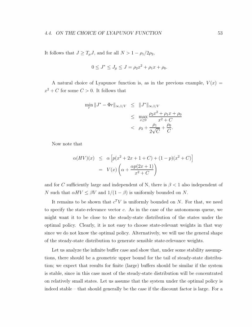
4.4. ON THE CHOICE OF LYAPUNOV FUNCTION 53
It follows that J ≥ TµJ , and for all N > 1− ρ1/2ρ2,
0 ≤ J∗ ≤ Jµ ≤ J = ρ2x2 + ρ1x+ ρ0.
A natural choice of Lyapunov function is, as in the previous example, V (x) =
x2 + C for some C > 0. It follows that
minr‖J∗ − Φr‖∞,1/V ≤ ‖J∗‖∞,1/V
≤ maxx≥0
ρ2x2 + ρ1x+ ρ0
x2 + C
< ρ2 +ρ1
2√C
+ρ0
C.
Now note that
α(HV )(x) ≤ α[p(x2 + 2x+ 1 + C) + (1− p)(x2 + C)
]
= V (x)
(α +
αp(2x+ 1)
x2 + C
)
and for C sufficiently large and independent of N, there is β < 1 also independent of
N such that αHV ≤ βV and 1/(1− β) is uniformly bounded on N .
It remains to be shown that cTV is uniformly bounded on N . For that, we need
to specify the state-relevance vector c. As in the case of the autonomous queue, we
might want it to be close to the steady-state distribution of the states under the
optimal policy. Clearly, it is not easy to choose state-relevant weights in that way
since we do not know the optimal policy. Alternatively, we will use the general shape
of the steady-state distribution to generate sensible state-relevance weights.
Let us analyze the infinite buffer case and show that, under some stability assump-
tions, there should be a geometric upper bound for the tail of steady-state distribu-
tion; we expect that results for finite (large) buffers should be similar if the system
is stable, since in this case most of the steady-state distribution will be concentrated
on relatively small states. Let us assume that the system under the optimal policy is
indeed stable – that should generally be the case if the discount factor is large. For a
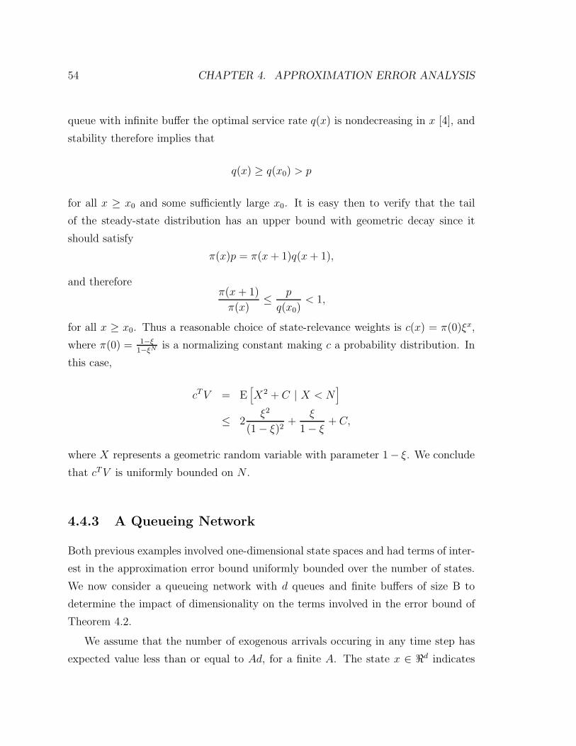
54 CHAPTER 4. APPROXIMATION ERROR ANALYSIS
queue with infinite buffer the optimal service rate q(x) is nondecreasing in x [4], and
stability therefore implies that
q(x) ≥ q(x0) > p
for all x ≥ x0 and some sufficiently large x0. It is easy then to verify that the tail
of the steady-state distribution has an upper bound with geometric decay since it
should satisfy
π(x)p = π(x+ 1)q(x+ 1),
and thereforeπ(x+ 1)
π(x)≤ p
q(x0)< 1,
for all x ≥ x0. Thus a reasonable choice of state-relevance weights is c(x) = π(0)ξx,
where π(0) = 1−ξ1−ξN is a normalizing constant making c a probability distribution. In
this case,
cTV = E[X2 + C | X < N
]
≤ 2ξ2
(1− ξ)2+
ξ
1− ξ+ C,
where X represents a geometric random variable with parameter 1− ξ. We conclude
that cTV is uniformly bounded on N .
4.4.3 A Queueing Network
Both previous examples involved one-dimensional state spaces and had terms of inter-
est in the approximation error bound uniformly bounded over the number of states.
We now consider a queueing network with d queues and finite buffers of size B to
determine the impact of dimensionality on the terms involved in the error bound of
Theorem 4.2.
We assume that the number of exogenous arrivals occuring in any time step has
expected value less than or equal to Ad, for a finite A. The state x ∈ <d indicates
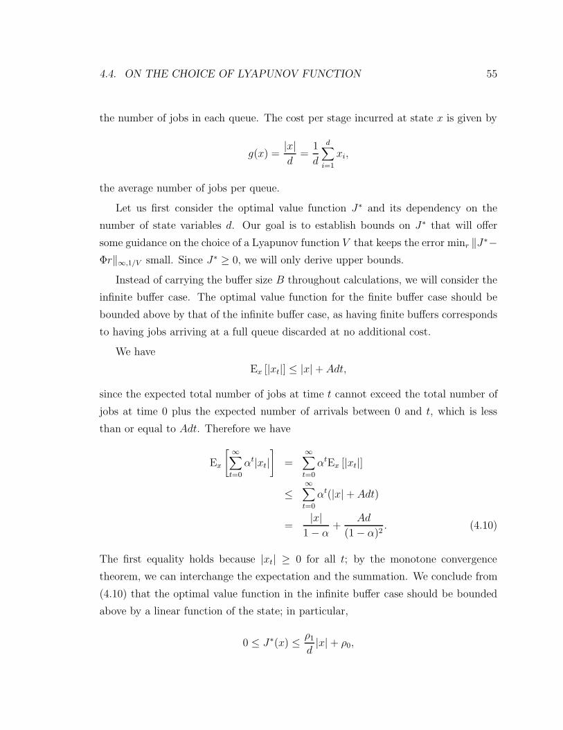
4.4. ON THE CHOICE OF LYAPUNOV FUNCTION 55
the number of jobs in each queue. The cost per stage incurred at state x is given by
g(x) =|x|d
=1
d
d∑i=1
xi,
the average number of jobs per queue.
Let us first consider the optimal value function J∗ and its dependency on the
number of state variables d. Our goal is to establish bounds on J∗ that will offer
some guidance on the choice of a Lyapunov function V that keeps the error minr ‖J∗−Φr‖∞,1/V small. Since J∗ ≥ 0, we will only derive upper bounds.
Instead of carrying the buffer size B throughout calculations, we will consider the
infinite buffer case. The optimal value function for the finite buffer case should be
bounded above by that of the infinite buffer case, as having finite buffers corresponds
to having jobs arriving at a full queue discarded at no additional cost.
We have
Ex [|xt|] ≤ |x|+ Adt,
since the expected total number of jobs at time t cannot exceed the total number of
jobs at time 0 plus the expected number of arrivals between 0 and t, which is less
than or equal to Adt. Therefore we have
Ex
[ ∞∑t=0
αt|xt|]
=∞∑t=0
αtEx [|xt|]
≤∞∑t=0
αt(|x|+ Adt)
=|x|
1− α+
Ad
(1− α)2. (4.10)
The first equality holds because |xt| ≥ 0 for all t; by the monotone convergence
theorem, we can interchange the expectation and the summation. We conclude from
(4.10) that the optimal value function in the infinite buffer case should be bounded
above by a linear function of the state; in particular,
0 ≤ J∗(x) ≤ ρ1
d|x|+ ρ0,
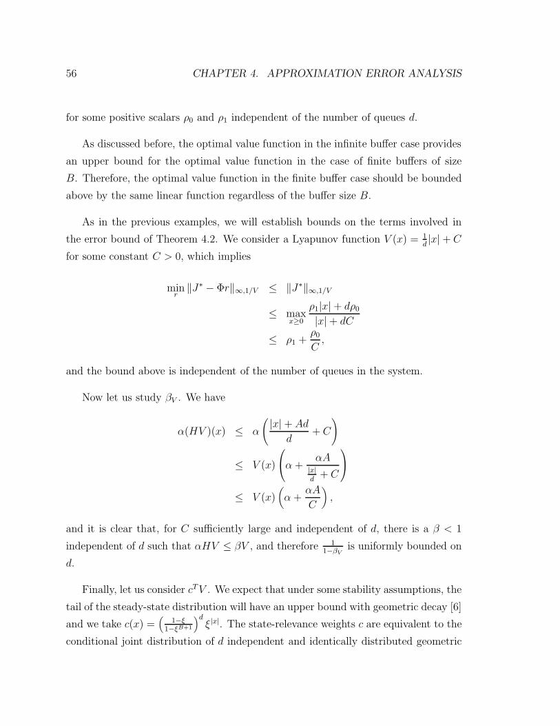
56 CHAPTER 4. APPROXIMATION ERROR ANALYSIS
for some positive scalars ρ0 and ρ1 independent of the number of queues d.
As discussed before, the optimal value function in the infinite buffer case provides
an upper bound for the optimal value function in the case of finite buffers of size
B. Therefore, the optimal value function in the finite buffer case should be bounded
above by the same linear function regardless of the buffer size B.
As in the previous examples, we will establish bounds on the terms involved in
the error bound of Theorem 4.2. We consider a Lyapunov function V (x) = 1d|x|+ C
for some constant C > 0, which implies
minr‖J∗ − Φr‖∞,1/V ≤ ‖J∗‖∞,1/V
≤ maxx≥0
ρ1|x|+ dρ0
|x|+ dC
≤ ρ1 +ρ0
C,
and the bound above is independent of the number of queues in the system.
Now let us study βV . We have
α(HV )(x) ≤ α
( |x|+ Ad
d+ C
)
≤ V (x)
α +
αA|x|d
+ C
≤ V (x)(α +
αA
C
),
and it is clear that, for C sufficiently large and independent of d, there is a β < 1
independent of d such that αHV ≤ βV , and therefore 11−βV
is uniformly bounded on
d.
Finally, let us consider cTV . We expect that under some stability assumptions, the
tail of the steady-state distribution will have an upper bound with geometric decay [6]
and we take c(x) =(
1−ξ1−ξB+1
)dξ|x|. The state-relevance weights c are equivalent to the
conditional joint distribution of d independent and identically distributed geometric
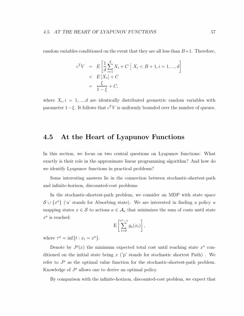
4.5. AT THE HEART OF LYAPUNOV FUNCTIONS 57
random variables conditioned on the event that they are all less than B+1. Therefore,
cTV = E
[1
d
d∑i=1
Xi + C∣∣∣ Xi < B + 1, i = 1, ..., d
]
< E [X1] + C
=ξ
1− ξ+ C,
where Xi, i = 1, ..., d are identically distributed geometric random variables with
parameter 1−ξ. It follows that cTV is uniformly bounded over the number of queues.
4.5 At the Heart of Lyapunov Functions
In this section, we focus on two central questions on Lyapunov functions: What
exactly is their role in the approximate linear programming algorithm? And how do
we identify Lyapunov functions in practical problems?
Some interesting answers lie in the connection between stochastic-shortest-path
and infinite-horizon, discounted-cost problems.
In the stochastic-shortest-path problem, we consider an MDP with state space
S ∪ {xa} (‘a’ stands for Absorbing state). We are interested in finding a policy u
mapping states x ∈ S to actions a ∈ Ax that minimizes the sum of costs until state
xa is reached:
E
[τa−1∑t=0
gu(xt)
],
where τa = inf{t : xt = xa}.Denote by Jp(x) the minimum expected total cost until reaching state xa con-
ditioned on the initial state being x (’p’ stands for stochastic shortest Path) . We
refer to Jp as the optimal value function for the stochastic-shortest-path problem.
Knowledge of Jp allows one to derive an optimal policy.
By comparison with the infinite-horizon, discounted-cost problem, we expect that
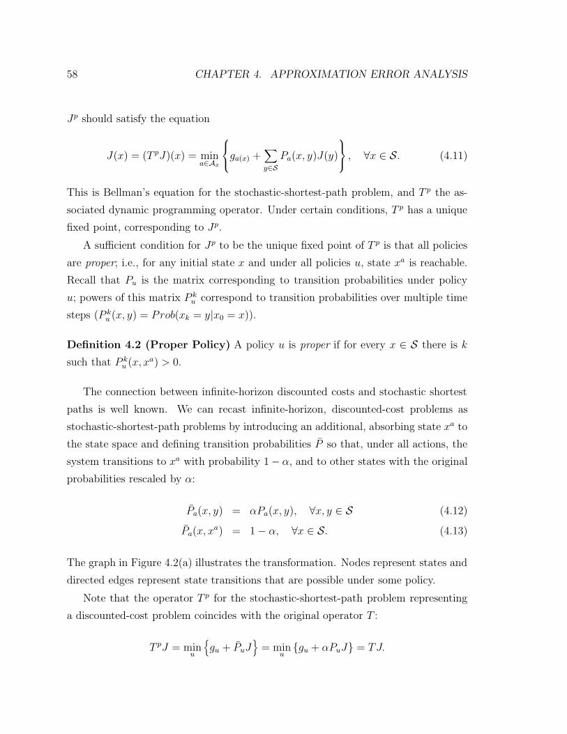
58 CHAPTER 4. APPROXIMATION ERROR ANALYSIS
Jp should satisfy the equation
J(x) = (T pJ)(x) = mina∈Ax
ga(x) +
∑y∈S
Pa(x, y)J(y)
, ∀x ∈ S. (4.11)
This is Bellman’s equation for the stochastic-shortest-path problem, and T p the as-
sociated dynamic programming operator. Under certain conditions, T p has a unique
fixed point, corresponding to Jp.
A sufficient condition for Jp to be the unique fixed point of T p is that all policies
are proper; i.e., for any initial state x and under all policies u, state xa is reachable.
Recall that Pu is the matrix corresponding to transition probabilities under policy
u; powers of this matrix P ku correspond to transition probabilities over multiple time
steps (P ku (x, y) = Prob(xk = y|x0 = x)).
Definition 4.2 (Proper Policy) A policy u is proper if for every x ∈ S there is k
such that P ku (x, xa) > 0.
The connection between infinite-horizon discounted costs and stochastic shortest
paths is well known. We can recast infinite-horizon, discounted-cost problems as
stochastic-shortest-path problems by introducing an additional, absorbing state xa to
the state space and defining transition probabilities P so that, under all actions, the
system transitions to xa with probability 1− α, and to other states with the original
probabilities rescaled by α:
Pa(x, y) = αPa(x, y), ∀x, y ∈ S (4.12)
Pa(x, xa) = 1− α, ∀x ∈ S. (4.13)
The graph in Figure 4.2(a) illustrates the transformation. Nodes represent states and
directed edges represent state transitions that are possible under some policy.
Note that the operator T p for the stochastic-shortest-path problem representing
a discounted-cost problem coincides with the original operator T :
T pJ = minu
{gu + PuJ
}= min
u{gu + αPuJ} = TJ.
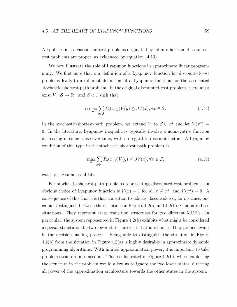
4.5. AT THE HEART OF LYAPUNOV FUNCTIONS 59
All policies in stochastic-shortest-problems originated by infinite-horizon, discounted-
cost problems are proper, as evidenced by equation (4.13).
We now illustrate the role of Lyapunov functions in approximate linear program-
ming. We first note that our definition of a Lyapunov function for discounted-cost
problems leads to a different definition of a Lyapunov function for the associated
stochastic-shortest-path problem. In the original discounted-cost problem, there must
exist V : S 7→ <+ and β < 1 such that
αmaxa
∑y∈S
Pa(x, y)V (y) ≤ βV (x), ∀x ∈ S. (4.14)
In the stochastic-shortest-path problem, we extend V to S ∪ xa and let V (xa) =
0. In the literature, Lyapunov inequalities typically involve a nonnegative function
decreasing in some sense over time, with no regard to discount factors. A Lyapunov
condition of this type in the stochastic-shortest-path problem is
maxa
∑y∈S
Pa(x, y)V (y) ≤ βV (x), ∀x ∈ S, (4.15)
exactly the same as (4.14).
For stochastic-shortest-path problems representing discounted-cost problems, an
obvious choice of Lyapunov function is V (x) = 1 for all x 6= xa, and V (xa) = 0. A
consequence of this choice is that transition trends are disconsidered; for instance, one
cannot distinguish between the situations in Figures 4.2(a) and 4.2(b). Compare these
situations. They represent state transition structures for two different MDP’s. In
particular, the system represented in Figure 4.2(b) exhibits what might be considered
a special structure: the two lower states are visited at most once. They are irrelevant
in the decision-making process. Being able to distinguish the situation in Figure
4.2(b) from the situation in Figure 4.2(a) is highly desirable in approximate dynamic
programming algorithms. With limited approximation power, it is important to take
problem structure into account. This is illustrated in Figure 4.2(b), where exploiting
the structure in the problem would allow us to ignore the two lower states, directing
all power of the approximation architecture towards the other states in the system.
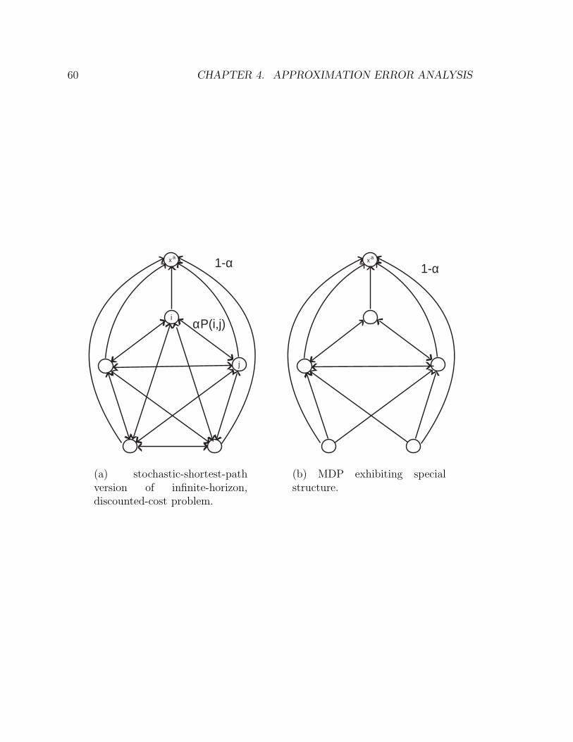
60 CHAPTER 4. APPROXIMATION ERROR ANALYSIS
1-αxa
j
i αP(i,j)
(a) stochastic-shortest-pathversion of infinite-horizon,discounted-cost problem.
1-αxa
(b) MDP exhibiting specialstructure.
4.5. AT THE HEART OF LYAPUNOV FUNCTIONS 61
Using the Lyapunov function as suggested by Theorem 4.2 does exactly that. Con-
sider once again the problem in Figure 4.2(b). Since there are no transitions to the
two lower states, they can be assigned arbitrarily large values in the Lyapunov func-
tion, and approximation errors in those state are highly discounted. Approximation
errors in those states are irrelevant, and this is captured by Theorem 4.2.
We now turn to the question of how to generate Lyapunov functions for practi-
cal problems. Although approximate linear programming does not require that we
explicitly provide Lyapunov functions — the bound in Theorem 4.2 holds as long as
there is a Lyapunov function in the span of the basis functions — knowing how to
generate them may aid in the process of selection of basis functions.
The following result, standard in dynamic programming, is of particular relevance
to our study of Lyapunov functions. It states that for stochastic-shortest-path prob-
lems in which that all policies are proper, the associated operator T p is a weighted-
maximum-norm contraction.
Theorem 4.3. Let T p be the dynamic programming operator for a stochastic-shortest-
path problem such that all policies are proper. Then there is ξ : S 7→ <+ and β < 1
such that for all J : S 7→ < and J : S 7→ <,
‖T pJ − T pJ‖∞,ξ ≤ β‖J − J‖∞,ξ.
The next theorem represents a modified version of an argument commonly used
in proving Theorem 4.3 [4]. It provides insight on the connection between Lyapunov
functions and the maximum-norm-contraction property. It also provides ideas on how
to generate Lyapunov functions.
Theorem 4.4. Let T p be the dynamic programming operator for a stochastic-shortest-
path problem such that all policies are proper. Consider the auxiliary problem of max-
imizing the sum of costs g(x) until state x∗ is reached, for an arbitrary positive cost
function g : S 7→ <+. Denote the maximum expected sum of costs conditioned on the
initial state being x by Jm(x) (‘m’ stands for Maximum costs). Then:
1. Jm is a Lyapunov function, in the sense of inequality (4.15).
62 CHAPTER 4. APPROXIMATION ERROR ANALYSIS
2. Theorem 4.3 holds with
ξ(·) = 1/Jm(·) (4.16)
and
β = maxx
Jm(x)− g(x)
Jm(x). (4.17)
Proof: Since all policies are proper, Jm is well-defined over S and given by equation
J(x) = g(x) + maxa∈Ax
∑y∈S
Pa(x, y)J(y).
It follows that
maxa∈Ax
∑y∈S
Pa(x, y)Jm(y) = Jm(x)− g(x)
≤ βJm(x). (4.18)
and the first claim follows. Recalling the definition of ξ (4.16), we have
(T pJ)(x)− (T pJ)(x) ≤ maxa∈Ax
∑y∈S
Pa(x, y)|J(y)− J(y)|
= maxa∈Ax
∑y∈S
Pa(x, y)Jm(y)ξ(y)|J(y)− J(y)|
≤ ‖J − J‖∞,ξ maxa∈Ax
∑y∈S
Pa(x, y)Jm(y)
≤ ‖J − J‖∞,ξβJm(x).
Since J and J are arbitrary, we conclude that
|(T pJ)(x)− (T pJ)(x)| ≤ ‖J − J‖∞,ξβJm(x), ∀x
ξ(x)|(T pJ)(x)− (T pJ)(x)| ≤ ‖J − J‖∞,ξβ, ∀x‖T pJ − T pJ‖∞,ξ ≤ β‖J − J‖∞,ξ,
and the second claim follows.
4.5. AT THE HEART OF LYAPUNOV FUNCTIONS 63
Theorem 4.4 suggests the following algorithm for automatically generating a Lya-
punov function for infinite-horizon, discounted-cost problems:
1. choose a positive cost function g : S 7→ <+;
2. find the optimal value function Jm for the problem of maximizing the discounted-
cost over infinite horizon. Jm is a Lyapunov function.
At first sight, the algorithm may appear ludicrous: trying to generate approximations
for the optimal value function for a minimum discounted-cost problem because com-
puting the exact function is infeasible, we require exact solution of a similar problem,
with the same intractable dimensions! However, two observations lead us to believe
that identifying Lyapunov functions may be an easier problem. First, the cost func-
tion g is to some extent arbitrary, and we may be able to choose it so that finding the
associated optimal value function becomes easy. Second, and more importantly, it is
easy to verify that scoring functions generated by approximate linear programming
as approximations to the optimal value function Jm are also Lyapunov functions. In
fact, a scoring function Jm generated by approximate linear programming satisfies
Jm ≥ TmJm = maxu{g + αPutildeJ
m} > αHJm.
Note that the inequality Jm ≥ TmJm is reversed relative to the customary inequality
T ≤ TJ in the LP’s involved in cost minimization; the difference is that here we are
considering a problem of cost maximization instead.
It is important to note that using this algorithm does require some thought about
the choice of g, as it influences the scaling properties of the contraction factor β (4.17)
and the quality of the Lyapunov function being generated. For instance, choosing g
to be a constant function immediately yields a Lyapunov function that is a constant;
however, that takes us back to the undesirable bound in Theorem 4.1.
It is not difficult to verify that Theorem 4.1 is a special case of Theorem 4.2;
it corresponds to having a Lyapunov function that is constant over the state space.
From Theorem 4.3, it is not difficult to show how to go in the opposite direction and
generalize Theorem 4.1 to obtain Theorem 4.2. Recall that the operator T associated
64 CHAPTER 4. APPROXIMATION ERROR ANALYSIS
with discounted-cost problems coincides with the operator T p associated with the
corresponding stochastic-shortest-path problem. We conclude that T is a weighted-
maximum-norm contraction. The proof of Theorem 4.1 revolves around the fact that
T is a unweighted-maximum-norm contraction; making the appropriate changes to
use the weighted-maximum-norm-contraction property instead, we obtain Theorem
4.2.
The unweighted-maximum-norm-contraction property of operator T is a key result
in dynamic programming, leading to a number of other important results, such as exis-
tence and uniqueness of the optimal value function, and convergence of value iteration.
It is therefore not surprising that, in the design and analysis of approximate dynamic
programming algorithms, this property has often been a central focus. The discussion
in this section demonstrates that using Lyapunov functions in the approximate lin-
ear programming algorithm corresponds to exploiting the weighted-maximum-norm-
contraction property of operator T , a generalization of the unweighted-maximum-
norm-contraction property, and exposes some of the limitations of the latter. We
expect that this insight will transcend its usefulness in approximate linear program-
ming and potentially guide the design and analysis of other approximate dynamic
programming algorithms.
Chapter 5
Constraint Sampling
The number of variables involved in the approximate LP is relatively small. However,
the number of constraints — one per state-action pair — can be intractable, and this
presents an obstacle. In this chapter, we study a constraint sampling scheme that
selects a tractable subset of constraints. We define an auxiliary LP with the same
variables and objective as the approximate LP, but with only the sampled subset
of constraints. More specifically, we aim at generating a good approximation to the
solution of the approximate LP by solving the problem
maxr cT Φr (5.1)
s.t. (TaΦr)(x) ≥ (Φr)(x) ∀(x, a) ∈ X ,
for some set X of state-action pairs. We refer to problem (5.1) as the reduced LP.
The reduced LP is motivated by the fact that, because there is a relatively small
number of variables in the approximate LP, many of the constraints should have a
minor impact on the feasible region and do not need to be considered. In particular,
we show that, by sampling a tractable number of constraints, we can guarantee that
the solution of the auxiliary LP will be near-feasible, with high probability.
The fact that constraint sampling yields near-feasible solutions is a general prop-
erty of LP’s with a large number of constraints and relatively few variables. Exploiting
65
66 CHAPTER 5. CONSTRAINT SAMPLING
properties specific to approximate linear programming, we will also establish that, un-
der certain conditions, the error in approximating the optimal value function yielded
by reduced LP should be close to that yielded by the approximate LP, with high
probability.
The remainder of the chapter is organized as follows. In Section 5.1, we motivate
the use of sampling in approximate linear programming, studying the possible conse-
quences of discarding some of the constraints. In Section 5.2, we establish bounds on
the number of constraints to be sampled so that the resulting reduced LP yields near-
feasible solutions. We provide bounds that relate the approximation error yielded by
the reduced LP to that yielded by the approximate LP in Section 5.3. Section 5.4
contains closing remarks.
In this chapter we consider certain families of MDP’s and dynamic programming
operators associated with them. We reserve the notation T for the dynamic program-
ming operator associated with the standard MDP (S,A·, P·(·, ·), g(·), α) considered
in previous chapter.
5.1 Relaxing the Approximate LP Constraints
In this section, we offer an interpretation for the optimal solution of the reduced LP.
The key observation is that its solution is also the solution to an approximate LP
related to another MDP. We investigate the differences between this new MDP and
the original one to understand the behavior of the reduced LP and gain insight into
which constraints in the approximate LP are most likely to be important.
We begin by introducing the notion of effective cost.
Definition 5.1 For any r ∈ <k, we define the effective costs associated with r by
gra(x) = max
ga(x), (Φr)(x)− α
∑y∈S
Pa(x, y)(Φr)(y)
.
Based on this definition, it is easy to show that a vector r is always feasible for
the approximate LP associated with the MDP (S,A·, P·(·, ·), gr· (·), α).
5.1. RELAXING THE APPROXIMATE LP CONSTRAINTS 67
We use (·)+ and (·)− to represent the positive and negative part functions:
(x)+ = max(x, 0) and (x)− = (−x)+.
Lemma 5.1. Let r ∈ <k be an arbitrary vector and gr· (·) the associated effective cost.
Then:
1. For any policy u, gru − gu ≤ (Φr − TΦr)+.
2. If T is the dynamic programming operator for the MDP (S,A·, P·(·, ·), gr· (·), α),
we have TΦr ≥ Φr.
Proof:
1. For any state-action pair (x, a), we have
gra(x)− ga(x) = max(ga(x), (Φr)(x)− α
∑y∈S
Pa(x, y)(Φr)(y))− ga(x)
= max((Φr)(x)− ga(x)− α∑y∈S
Pa(x, y)(Φr)(y), 0)
≤ max((Φr)(x)− (TΦr)(x), 0).
2. If a and x are such that
ga(x) + α∑y∈S
Pa(x, y)(Φr)(y) ≥ (Φr)(x),
then we have gra(x) = ga(x) and
gra(x) + α
∑y∈S
Pa(x, y)(Φr)(y) ≥ (Φr)(x).
Otherwise, we have
gra(x) = (Φr)(x)− α
∑y∈S
Pa(x, y)(Φr)(y),
gra(x) + α
∑y∈S
Pa(x, y)(Φr)(y) = (Φr)(x).
68 CHAPTER 5. CONSTRAINT SAMPLING
We can use Lemma 5.1 to interpret the solution of the reduced LP.
Lemma 5.2. Let r be the optimal solution of the reduced LP. Define T to be the dy-
namic programming operator associated with the MDP given by (S,A·, P·(·, ·), gr· (·), α).
Then r is also the optimal solution of
maxr cT Φr (5.2)
s.t. (TΦr)(x) ≥ (Φr)(x) ∀x ∈ S.
Proof: From Lemma 5.1 (ii), the optimal solution r of the reduced LP is feasible
for problem (5.2). Therefore, it suffices to show that the feasible region of (5.2) is
contained in that of the reduced LP. Take any r that is feasible for (5.2). Then, for
all (x, a) ∈ X ,
(Φr)(x) ≤ gra(x) + α
∑y∈S
Pa(x, y)(Φr)(y)
= ga(x) + α∑y∈S
Pa(x, y)(Φr)(y),
and r is feasible for the reduced LP. The equality holds because ga(x) = gra(x) for all
(x, a) ∈ X . We conclude that the feasible region of the reduced LP contains that of
(5.2), completing the proof.
Lemma 5.2 establishes that we can view the reduced LP as effectively trying to
approximate the optimal value function of an MDP with potentially larger costs than
those in the original MDP. We can expect it to be a reasonable approximation to
the approximate LP as long as the optimal value function associated with the MDP
(S,A·, P·(·, gr· (·), ·, α) is close to J∗. The next lemma establishes a bound on the
difference between optimal value functions for problems that are equal except for
their costs.
Lemma 5.3. Let T be the dynamic programming operator associated with an MDP
(S,A·, P·(·, ·), g·(·), α), where gu ≥ gu for all u. Let J∗ and J be the fixed points of T
and T , respectively. Then if u∗ is any optimal policy associated with the MDP related
5.1. RELAXING THE APPROXIMATE LP CONSTRAINTS 69
to T , we have
J(x)− J∗(x) ≤∑y
d(x, y)(gu∗(y)− gu∗(y)), (5.3)
where
d(x, y) =∞∑t=0
αtP tu∗(x, y). (5.4)
Furthermore, if π is a stationary state distribution associated with u∗ (π = πPu∗), we
have
‖J − J∗‖1,π ≤ 1
1− α‖gu∗ − gu∗‖1,π. (5.5)
Proof: Let u be an optimal policy with respect to T . Then
J(x)− J∗(x) =∞∑
t=0
αt∑y∈S
P tu(x, y)gu(y)−
∞∑t=0
αt∑y∈S
P tu∗(x, y)gu∗(y)
≤∞∑
t=0
αt∑y∈S
P tu∗(x, y)gu∗(y)−
∞∑t=0
αt∑y∈S
P tu∗(x, y)gu∗(y)
=∑y∈S
(gu∗(y)− gu∗(y))∞∑
t=0
αtP nu∗(x, y),
and (5.3) follows. Note that the inequality holds because
Ju∗ =∞∑
t=0
αtP tu∗ gu∗ ≥ Ju =
∞∑t=0
αtP tugu,
since u is optimal for the dynamic program with costs g.
From (5.3) we get
‖J − J∗‖1,π = Eπ|J(X0)− J∗(X0)|≤ Eπ
[ ∞∑t=0
αtP tu∗(gu∗ − gu∗)
]
=∞∑
t=0
αtEπ [gu∗(Xt)− gu∗(Xt)]
=∞∑
t=0
αtEπ [gu∗(X0)− gu∗(X0)]
=1
1− α‖gu∗ − gu∗‖1,π,
70 CHAPTER 5. CONSTRAINT SAMPLING
where the second equality holds by the nonnegativity of gu∗ − gu∗ and the monotone
convergence theorem and the third equality holds because π is a stationary distribu-
tion associated with Pu∗ .
As discussed in Chapters 3 and 4, it seems sensible to emphasize approximation
errors in different states according to how often they are visited. The rationale is
that non-optimal actions should typically increase costs more significantly if they are
taken in frequently visited states than in rarely visited ones. Note that the bound
(5.5) involves a norm that weights states according to their relative frequencies under
an optimal policy, therefore it seems to be a reasonable measure for the error incurred
by using the reduced LP instead of the approximate LP.
Together, Lemmas 5.2 and 5.3 provide some intuition for choices of constraints
to be included in the reduced LP. From Lemma 5.2, we see that the reduced LP
can be viewed as the approximate LP for a different problem, with potentially larger
costs in some of the non-sampled states. We expect that, the closer the optimal
value functions associated with the new and the original problems are, the more the
reduced LP’s behavior will resemble that of the approximate LP. Therefore, a sensible
approach might be to design the constraint sampling scheme so as to minimize the
error bounds presented in Lemma 5.3. These bounds suggest that some constraints
are more important than others:
• The error gra(x) − ga(x) is equal to zero for state-action pairs (x, a) such that
ga(x) + α∑
y∈S Pa(x, y)(Φr)(y) ≥ (Φr)(x); in particular, costs remain the same
for state-action pairs whose constraints are included in the reduced LP. There-
fore the expected difference between the optimal value functions (5.5), which
is shown to be proportional to the expected difference between the one-stage
costs, may be reduced by choosing X to include states x with higher stationary
probability.
• The componentwise bound (5.3) establishes that the difference between effective
costs and original costs in a state y does not affect all states equally; its impact
on each state x depends on the metric d(x, y). If we want to minimize errors in
the region of the state space that is visited more frequently, it seems reasonable
5.2. HIGH-CONFIDENCE SAMPLING FOR LINEAR CONSTRAINTS 71
to sample states that are “far” from this region with smaller probability. This
translates into a sampling scheme that emphasizes frequently visited states.
Indeed, the metric d(x, y) can be interpreted as the average number of visits to
state y given that the initial state is x and the system operates under an optimal
policy, and therefore if a state is visited frequently, we expect that states that
are “close” to it should also be visited frequently, and states that are “far” from
it should probably be visited rarely.
We have identified an important property of the approximate LP, namely, that
not all constraints are equally relevant, and their relative relevance depends on how
often their corresponding states are visited. In the next section, we will show how
to draw samples from a set of linear constraints that have an associated measure of
relative importance so as to ensure with high confidence that any vector that satisfies
the sampled constraints is near-feasible — it violates at most a set of constraints
that has small measure. The results of Section 5.2 will then be applied in Section
5.3 to establish a bound on the error associated with the reduced LP, relative to the
approximate LP, when constraints are randomly sampled.
5.2 High-Confidence Sampling for Linear Constraints
We consider a set of linear constraints
Azr + bz ≥ 0, ∀z ∈ Z (5.6)
where r ∈ <k and Z is a generic set of constraint indices. To keep the exposition
simple, we make the following assumption on Z:
Assumption 5.1. The set of constraint indices Z is finite or countable.
This assumption is sufficient for our purposes, since we consider MDP’s with finite
state and action spaces.
We use Ar + b as shorthand notation for the function fr(z) = Azr + bz .
Motivated by the approximate LP setting, we assume that k � |Z|. Hence we
have relatively few variables and a possibly huge number of constraints. In such a
72 CHAPTER 5. CONSTRAINT SAMPLING
situation, we expect that many of the constraints will be irrelevant, either because
they are always inactive or because they have a minor impact on the feasible region.
One might then speculate that the feasible region specified by all constraints can be
well-approximated by a sampled subset of these constraints. In the sequel, we will
show that this is indeed the case, at least with respect to a certain criterion for a
“good” approximation. We will also show that the number of constraints necessary to
guarantee a good approximation does not depend on the total number of constraints,
but rather on the number of variables.
We start by specifying how constraints are sampled. We assume that there is
a probability measure ψ on Z. The distribution ψ will have a dual role in our
approximation scheme: on one hand, constraints will be sampled according to ψ; on
the other hand, the same distribution will be involved in the criterion for assessing
the quality of a particular set of sampled constraints. We have seen that in the
approximate linear programming method certain constraints are more likely to have
a significant impact on the final approximation we are trying to generate than others.
In that context, ψ would be chosen to capture this fact, so that more important
constraints are selected with higher probability.
We now discuss what it means for a certain set of sampled constraints to be good.
Note that in general we cannot guarantee that all constraints will be satisfied over the
feasible region of any subset of constraints. In Figure 5.1, for instance, we exemplify a
worst-case scenario in which it is necessary to include all constraints in order to ensure
that all of them are satisfied. Note however that the impact of any one of them on the
feasible region is minor and might be considered negligible. In this spirit, we consider
a subset of constraints good if we can guarantee that, by satisfying this subset, the
set of constraints that are not satisfied has small measure. In other words, given a
tolerance parameter 0 < ε < 1, we want to have W ⊂ Z satisfying
supr:Azr+bz≥0, ∀z∈W
ψ ({y : Ayr + by < 0}) ≤ ε. (5.7)
Defining a set of constraint indices W to be good if (5.7) holds, we might ask how
many (possibly repeated) constraints have to be sampled in order to ensure that the
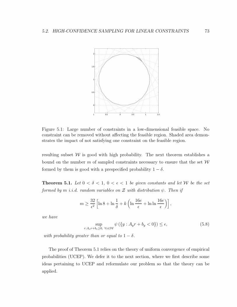
5.2. HIGH-CONFIDENCE SAMPLING FOR LINEAR CONSTRAINTS 73
1 0.5 0 0.5 1 1.5
0
0.5
1
1.5
2
Figure 5.1: Large number of constraints in a low-dimensional feasible space. Noconstraint can be removed without affecting the feasible region. Shaded area demon-strates the impact of not satisfying one constraint on the feasible region.
resulting subset W is good with high probability. The next theorem establishes a
bound on the number m of sampled constraints necessary to ensure that the set Wformed by them is good with a prespecified probability 1− δ.
Theorem 5.1. Let 0 < δ < 1, 0 < ε < 1 be given constants and let W be the set
formed by m i.i.d. random variables on Z with distribution ψ. Then if
m ≥ 32
ε2
[ln 8 + ln
1
δ+ k
(ln
16e
ε+ ln ln
16e
ε
)],
we have
supr:Azr+bz≥0, ∀z∈W
ψ ({y : Ayr + by < 0}) ≤ ε, (5.8)
with probability greater than or equal to 1− δ.
The proof of Theorem 5.1 relies on the theory of uniform convergence of empirical
probabilities (UCEP). We defer it to the next section, where we first describe some
ideas pertaining to UCEP and reformulate our problem so that the theory can be
applied.
74 CHAPTER 5. CONSTRAINT SAMPLING
5.2.1 Uniform Convergence of Empirical Probabilities
Consider a probability space (Z,Z, µ) and a class C = {Ci, i ∈ I} ⊂ Z, where I is
a given set of indices. One would like to estimate µ(Ci) by drawing samples from Zand observing whether they belong to Ci or not. Let z ∈ Zm be a vector containing
m samples. The fraction of samples belonging to a set Ci is called the empirical
probability of Ci and denoted by µ(Ci, z). The class C will have the UCEP property
if the empirical probabilities converge in probability to their true value, uniformly on
I as the number of samples m increases. Results determining when a given class has
this property and the associated convergence rate can be found in [20, 57].
Let us first recast our problem as one of UCEP. Consider the class
C = {Cr : r ∈ <k}, (5.9)
where
Cr = {z ∈ Z : Azr + bz ≥ 0} .
Note that Cr is the set of indices of constraints that are satisfied by r. For any
vector r, we can determine the empirical probability ψ of Cr by drawing a sequence
of m samples of constraint indices collected in a vector z ∈ Zm according to ψ, and
setting
ψ(Cr, z) =1
m
m∑i=1
1Cr(zi),
where 1A is the indicator function of set A and zi is the ith component of z. If Chas the UCEP property, there is a minimum number of samples m0 that guarantees,
with high probability, that the true measure of any set in C is close to the empirical
measure.
To see how UCEP can be applied to the constraint sampling problem, note that,
for any vector r that is feasible for the sampled constraints, we have ψ(Cr) = 1.
Assuming that we have chosen the number of samples to ensure that ψ is close to ψ,
we conclude that for all such vectors, ψ(Cr) is close to 1 with high probability, hence
r is near-feasible.
The weak law of large numbers guarantees that, under certain conditions, the
5.2. HIGH-CONFIDENCE SAMPLING FOR LINEAR CONSTRAINTS 75
empirical probabilities will converge in probability to their true values for each r. The
questions to be asked are: Does ψr converge uniformly on r? What is the convergence
rate? The answers are closely related to a certain measure of the complexity of classes
of sets — the VC dimension [20, 57].
Definition 5.2 (VC dimension) Let (Z,Z) be a measurable space. Let A ⊂ Z be
a class of sets. The VC dimension of A, denoted dim(A), is the maximum integer n
such that there is a set P ⊂ A of cardinality n that is shattered by A, that is, such
that |{B ∩ P : B ∈ A}| = 2n.
The next two lemmas establish that for the class C defined in (5.9), we have
dim(C) ≤ k.
Lemma 5.4. [20] Let F be an m-dimensional vector space of real functions on a set
Z and g be any function on Z. Let C = {Cf : f ∈ F} be the class of sets of the form
Cf = {z ∈ Z : f(z) + g(z) ≥ 0}. Then dim(C) = m.
Lemma 5.5. Let C be as defined in (5.9). Then dim(C) ≤ k.
Proof: It is clear that the set {f : f(z) = Azr, r ∈ <k} forms a real vector space of
dimension at most k. Hence, by Lemma 5.5, dim(C) ≤ k.
The following lemma, adapted from [20, 57], establishes the rate of convergence of
empirical probabilities associated with a class of sets as a function of its VC dimension.
Lemma 5.6. Let (Z,Z, µ) be a probability space. Let A ⊂ Z be a class with finite
VC-dimension. For any vector z ∈ Zm and any set B ∈ A, define
µ(B, z) =1
m
M∑i=1
1B(zi).
Then
µm
({z ∈ Zm : sup
B∈A|µ(B)− µ(B, z)| > ε
})≤ 8
(16e
εln
16e
ε
)dim(A)
e−mε2
32 ,
where µm denotes the joint distribution for m i.i.d. random variables distributed
according to µ.
We are now poised to prove Theorem 5.1.

76 CHAPTER 5. CONSTRAINT SAMPLING
Proof of Theorem 5.1
Let C be as in (5.9). For any z ∈ Zm and any B ∈ C, define
ψ(B, z) =1
m
m∑i=1
1B(zi).
Then from Lemmas 5.5 and 5.6, we have
ψm
({z ∈ Zm : sup
r∈<d
∣∣∣ψ(Cr)− ψ(Cr, z)∣∣∣ > ε
})≤ 8
(16e
εln
16e
ε
)dim(C)
e−mε2
32
≤ 8(
16e
εln
16e
ε
)k
e−mε2
32 ,
where ψm denotes the joint distribution for m i.i.d. random variables distributed
according to ψ. Let W = {z1, ..., zm} and FW = {r : Az + bz ≥ 0, ∀z ∈ W}. We have
8(
16e
εln
16e
ε
)k
e−mε2
32 ≥ ψm
({z ∈ Zm : sup
r∈FW
∣∣∣ψ(Cr)− ψ(Cr, z)∣∣∣ > ε
})
= ψm
({z ∈ Zm : sup
r∈FW|ψ(Cr)− 1| > ε
})
= ψm
({z ∈ Zm : sup
r∈FW1− ψ(Cr) > ε
})
= ψm
({z ∈ Zm : sup
r∈FWψ(Cr) > ε
})
= ψm
({z ∈ Zm : sup
r∈FWψ({y ∈ Z : Ayr + by < 0}) > ε
}),
Hence by setting
m ≥ 32
ε2
[ln 8 + ln
1
δ+ k
(ln
16e
ε+ ln ln
16e
ε
)],
we conclude after some simple algebra that the bound (5.8) on the measure of the set
of the violated constraints holds with probability greater than or equal to 1− δ.
Theorem 5.1 establishes what may be perceived as a puzzling result: as the num-
ber of constraints grows, the number of sampled constraints necessary for a good
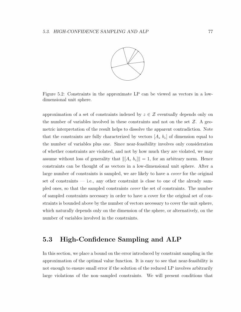
5.3. HIGH-CONFIDENCE SAMPLING AND ALP 77
Figure 5.2: Constraints in the approximate LP can be viewed as vectors in a low-dimensional unit sphere.
approximation of a set of constraints indexed by z ∈ Z eventually depends only on
the number of variables involved in these constraints and not on the set Z. A geo-
metric interpretation of the result helps to dissolve the apparent contradiction. Note
that the constraints are fully characterized by vectors [Az bz ] of dimension equal to
the number of variables plus one. Since near-feasibility involves only consideration
of whether constraints are violated, and not by how much they are violated, we may
assume without loss of generality that ‖[Az bz]‖ = 1, for an arbitrary norm. Hence
constraints can be thought of as vectors in a low-dimensional unit sphere. After a
large number of constraints is sampled, we are likely to have a cover for the original
set of constraints — i.e., any other constraint is close to one of the already sam-
pled ones, so that the sampled constraints cover the set of constraints. The number
of sampled constraints necessary in order to have a cover for the original set of con-
straints is bounded above by the number of vectors necessary to cover the unit sphere,
which naturally depends only on the dimension of the sphere, or alternatively, on the
number of variables involved in the constraints.
5.3 High-Confidence Sampling and ALP
In this section, we place a bound on the error introduced by constraint sampling in the
approximation of the optimal value function. It is easy to see that near-feasibility is
not enough to ensure small error if the solution of the reduced LP involves arbitrarily
large violations of the non–sampled constraints. We will present conditions that
78 CHAPTER 5. CONSTRAINT SAMPLING
enable a graceful error bound.
Our main result is based on the following variant of the reduced LP, which we
refer to as the bounded reduced LP:
max cT Φr (5.10)
s.t. (TaΦr)(x) ≥ (Φr)(x), ∀(x, a) ∈ Xr ∈ N .
The set N is viewed as another algorithm parameter to be chosen, like c and Φ. It
must contain an optimal solution of the approximate LP and is used for controlling
the magnitude of violations of nonsampled constraints. A more comprehensive expla-
nation of the constraint r ∈ N and appropriate selections for N will be discussed in
Section 5.3.1.
Let us introduce certain constants and functions involved in our error bound.
Recall the definition of µu,ν (3.1). We define a family of probability distributions µu
on the state space S, given by
µTu ≡ µT
u,c = (1− α)cT (I − αPu)−1, (5.11)
for each policy u. Note that
(I − αPu)−1 =
∞∑t=0
αtP tu,
and therefore, if c is a probability distribution, µu(x)/(1 − α) is the expected dis-
counted number of visits to state x under policy u, if the initial state is distributed
according to c. Furthermore, limα↑1 µu(x) is the stationary distribution associated
with policy u. We interpret µu as a measure of the relative importance of states
under policy u.
We can prove the following lemma involving µu.
5.3. HIGH-CONFIDENCE SAMPLING AND ALP 79
Lemma 5.7. For all J and p ≥ 1, we have
‖αPuJ‖p,µu ≤ ‖J‖p,µu.
Proof: We have
‖αPuJ‖pp,µu
= αp∑x
µu(x)
∣∣∣∣∣∣∑y∈S
Pu(x, y)J(y)
∣∣∣∣∣∣p
≤ αp∑x
µu(x)
∑
y∈SPu(x, y)|J(y)|
p
≤ αp∑x
µu(x)∑y∈S
Pu(x, y)|J(y)|p
= αpµTuPu|J |p
≤ α(1− α)cT∞∑t=0
αtP tuPu|J |p
= (1− α)cT∞∑t=1
αtP tu|J |p
≤ (1− α)cT∞∑t=0
αtP tu|J |p
= µTu |J |p
= ‖J‖pp,µu
.
The notation |J |p indicates componentwise absolute value and power of the vector J .
We used Jensen’s inequality on the first and second lines with the convex functions
|.| and xp, which is convex on <+ for all p ≥ 1. The third inequality follows from
αp ≤ α.
Define for each policy u and for each p the constant
Mu,p = max(supr∈N
‖Φr‖p,µu , ‖gu‖p,µu) (5.12)
and the distribution
ψu(x, a) =µu∗(x)
|Ax| , ∀a ∈ Ax,
80 CHAPTER 5. CONSTRAINT SAMPLING
and denote by A the maximum number of actions available for any given state:
A = maxx|Ax|.
We now present the main result of the chapter — a bound on the error introduced
by constraint sampling in the approximation of the optimal value function.
Theorem 5.2. Let N ⊂ <k be a set containing an optimal solution of the approx-
imate LP. Let u∗ be an optimal policy and X be a (random) set of m state-action
pairs sampled independently according to the distribution ψu∗(x, a), where
m ≥ 32A2
( (1−α)ε6
)2p
p−1
ln 8 + ln
1
δ+ k
ln
16Ae
( (1−α)ε6
)p
p−1
+ ln ln16Ae
( (1−α)ε6
)p
p−1
, (5.13)
for a given scalar p > 1. Let r be a solution to the approximate LP and r be a solution
to the bounded reduced LP. Then, with probability at least 1− δ, we have
‖J∗ − Φr‖1,c ≤ ‖J∗ − Φr‖1,c +Mu∗,pε. (5.14)
Proof: From Theorem 5.1, we have, with probability no less than 1− δ,
( (1−α)ε6
)p
p−1
A≥ ψu∗ ({(x, a) : (TaΦr)(x) < (Φr)(x)})
=∑x
µu∗(x)1
|Ax|∑a
1(TaΦr)(x)<(Φr)(x)
≥ 1
A
∑x
µu∗(x)1(Tu∗Φr)(x)<(Φr)(x), (5.15)
therefore for all q ≥ 1 we have
∥∥∥1(Tu∗Φr)(·)−(Φr)(·)<0
∥∥∥q
q,µu∗≤(
(1− α)ε
6
) pp−1
. (5.16)
5.3. HIGH-CONFIDENCE SAMPLING AND ALP 81
We also have
‖J∗ − Φr‖1,c = cT∣∣∣(I − αPu∗)
−1(gu∗ − (I − αPu∗)Φr)∣∣∣
≤ cT (I − αPu∗)−1 |gu∗ − (I − αPu∗)Φr|
= cT (I − αPu∗)−1[(gu∗ − (I − αPu∗)Φr)
+ + (gu∗ − (I − αPu∗)Φr)−]
= cT (I − αPu∗)−1[(gu∗ − (I − αPu∗)Φr)
+ − (gu∗ − (I − αPu∗)Φr)− +
+2 (gu∗ − (I − αPu∗)Φr)−]
= cT (I − αPu∗)−1[gu∗ − (I − αPu∗)Φr + 2 (Tu∗Φr − Φr)−
]= cT (J∗ − Φr) + 2cT (I − αPu∗)
−1 (Tu∗Φr − Φr)− . (5.17)
The inequality comes from the fact that c > 0 and
(I − αPu∗)−1 =
∞∑n=0
αnP nu∗ ≥ 0,
where the inequality is componentwise, so that
∣∣∣(I − αPu∗)−1(gu∗ − (I − αPu∗)Φr)
∣∣∣ ≤∣∣∣(I − αPu∗)
−1∣∣∣ |(gu∗ − (I − αPu∗)Φr)|
= (I − αPu∗)−1 |(gu∗ − (I − αPu∗)Φr)| .
We assume without loss of generality that r ∈ N , since by assumption there is
at least one optimal solution of the ALP that satisfies this constraint1. Therefore r
is feasible for the bounded reduced LP. Since r is the optimal solution of the same
problem, we have cT Φr ≥ cT Φr and
cT (J∗ − Φr) ≤ cT (J∗ − Φr)
= ‖J∗ − Φr‖1,c, (5.18)
hence we just need to show that the second term in (5.17) is small to guarantee that
problem (5.10) does not perform much worse than the approximate LP.
1Note that all optimal solutions of the approximate LP yield the same approximation error‖J∗ − Φr‖1,c, hence the error bound (5.14) is independent of the choice of r.
82 CHAPTER 5. CONSTRAINT SAMPLING
Now
2cT (I − αPu∗)−1 (Tu∗Φr − Φr)− = (5.19)
=2
1− αµT
u∗ (Tu∗Φr − Φr)−
=2
1− α
⟨Tu∗Φr − Φr, 1(Tu∗Φr)(·)−(Φr)(·)<0
⟩µu∗
≤ 2
1− α‖Tu∗Φr − Φr‖p,µu∗‖1(Tu∗Φr)(·)−(Φr)(·)<0‖ p
p−1,µu∗ , (5.20)
where the last step is an application of Holder’s inequality.
Applying (5.16) with q = pp−1
yields
‖1(Tu∗Φr)(·)−(Φr)(·)<0‖ pp−1
,µu∗ ≤(1− α)ε
6, (5.21)
with probability at least 1− δ.
Finally, we have
‖Tu∗Φr − Φr‖p,µu∗ ≤ ‖gu∗‖p,µu∗ + ‖Φr‖p,µu∗ + ‖αPu∗Φr‖p,µu∗
≤ ‖gu∗‖p,µu∗ + 2‖Φr‖p,µu∗ (5.22)
≤ 3Mu∗,p. (5.23)
The second inequality follows from Lemma 5.7, and the third one is follows from the
definition of Mu∗,p.
The error bound (5.14) follows from (5.17), (5.18), (5.20), (5.21) and (5.23).
If we think of the quantity Mu∗,p as an indicator of the magnitude of the func-
tions involved in the approximation scheme — the optimal value function and its
approximation, the error bound (5.14) implies that we can make the approximation
error yielded by the bounded reduced LP relatively close to that obtained by the
approximate LP, with a tractable number of sampled constraints.
Some aspects of Theorem 5.2 deserve further discussion. The first of them is the
constraint r ∈ N , which differentiates the bounded reduced LP from the reduced LP.
This constraint is discussed in Section 5.3.1. Another aspect relates to the sampling
5.3. HIGH-CONFIDENCE SAMPLING AND ALP 83
distribution ψu∗ . It is clear that we will not be able to compute and use it in practice.
We discuss in Section 5.3.2 how sampling with a different distribution affects our error
bounds. Finally, some difficulties may arise in problems involving a large number of
actions per state — our bounds require a number of samples on the order ofO(A2 lnA)
on the maximum number of available actions per state A. We address how deal with
large state spaces in Section 5.3.3.
5.3.1 Bounding Constraint Violations
The motivation for the bounded reduced LP is that constraint sampling alone only
guarantees near-feasibility, without regard to the magnitude of the violations of con-
straints that are not sampled. It is reasonable to expect that, the larger these vio-
lations are, the worse the approximation yielded by the reduced LP relative to that
of the approximate LP. Recall that the set N , involved in the bounded reduced LP,
affects the constant Mu∗,p present in the error bound (5.14). The constant Mu∗,p, in
turn, reflects how large vectors Φr involved in the approximation can be. The under-
lying idea is to choose N so as to keep approximations Φr produced by the bounded
reduced LP relatively small, thereby preventing constraint violations from growing
out of control.
Two important issues that affect the significance of the error bounds presented in
Theorem 5.2 are the magnitude of Mu∗,p and the feasibility of choosing an appropriate
set N efficiently. We will begin by investigating Mu∗,p.
Recall that Mu∗,p is defined as the maximum of supr∈N ‖Φr‖p,µu∗ and ‖gu∗‖p,µu∗ .
In our analysis, we focus on the first term; the implicit assumption is that typically
the magnitude of the optimal value function and its approximation is of the order of
1/(1− α) of the magnitude of one-stage costs, so that supr∈N ‖Φr‖p,µu∗ drives Mu∗,p.
The set N must contain an optimal solution of the approximate LP. Hence the
magnitude of the functions involved in the bounded reduced LP is at least in part
dictated by the behavior of the approximate LP. The next lemma provides a bound
on a certain norm of optimal solutions to the approximate LP.
84 CHAPTER 5. CONSTRAINT SAMPLING
Lemma 5.8. Let r be an optimal solution of the approximate LP. Then
‖Φr‖1,c ≤ 2‖J∗‖1,c. (5.24)
Proof: First, note that J∗ ≥ Φr and J∗ ≥ 0, therefore
cT (Φr)+ ≤ cTJ∗ = ‖J∗‖1,c. (5.25)
Since we assume that all costs are nonnegative, r = 0 is always a feasible solution for
the approximate LP, therefore
0 ≤ cT Φr
≤ cT (Φr)+ − cT (Φr)−,
and
cT (Φr)− ≤ cT (Φr)+. (5.26)
From (5.25) and (5.26):
‖Φr‖1,c = cT (Φr)+ + cT (Φr)−
≤ 2cT (Φr)+
≤ 2‖J∗‖1,c
and the claim follows.
Lemma 5.8 establishes that solutions to the approximate LP are comparable in
magnitude to the optimal value function J∗ — approximate LP solutions have norm
‖ · ‖1,c at most twice as large as J∗. Ideally, one would choose N so as to reproduce
that behavior in the bounded reduced LP; in other words, N would impose that the
approximations involved in the bounded reduced LP are on the same order of magni-
tude as the optimal value function. Note that, if c = πu, the stationary distribution
associated with policy u, ‖Ju‖1,c is equal to the average cost associated with policy
u multiplied by 1/(1 − α). Therefore, in rough terms, Mu∗,p is representative of the
5.3. HIGH-CONFIDENCE SAMPLING AND ALP 85
average cost of the system scaled by the factor 1/(1−α), at least for relatively small
values of p.
We now turn to the question of how to choose N . Appropriate choices will depend
on the problem at hand. Here we discuss three different approaches that are not
completely developed, but may represent a starting point in setting up the bounded
reduced LP for a practical application.
The simplest approach is to use the reduced LP in its original form, with con-
straints sampled randomly according to the distribution suggested in Theorem 5.2.
The hope is that the constraints relative to a large number of (random) state-action
pairs would eventually lead to a finite upper bound for any Φr satisfying them, as
any feasible solution of the approximate LP is bounded above by J∗. That being the
case, we may consider a bounded reduced LP containing the same constraints and
cT Φr ≥ 0, which is always satisfied by any optimal solution of the approximate LP or
of the reduced LP (recall that r = 0 is always feasible since costs are nonnegative).
Vectors Φr that are bounded above and satisfy this constraint must be bounded.
Therefore we may think of the sampled constraints and cT Φr ≥ 0 as a constraint of
the form r ∈ N , and Theorem 5.2 applies with a finite Mu∗,p. However, since the
constraint cT Φr ≥ 0 is always satisfied by optimal solutions of the reduced LP, we
conclude that the solutions of the reduced LP and of the bounded reduced LP un-
der consideration coincide, and the bounds provided in Theorem 5.2 for the bounded
reduced LP should hold for the reduced LP.
We expect the aforementioned approach to be effective in practice, but it certainly
lacks theoretical guarantees; in other words, it does not allow for a priori bounds
on the constant Mu∗,p. Having such bounds would make it possible to choose the
tolerance level ε — equivalently, the number of sampled constraints — so as to achieve
a prespecified error Mu∗,pε. In the absence of these bounds, one can at best solve the
reduced LP with a given ε and then estimate the constraint sampling error based
on the solution Φr, rather than control it. An alternative approach is as follows.
Along the same lines used to conclude that the constraints of the reduced LP should
eventually constitute a constraint of the form r ∈ N with the desired properties,
one could conjecture that, in some applications, it is possible to find a small set of
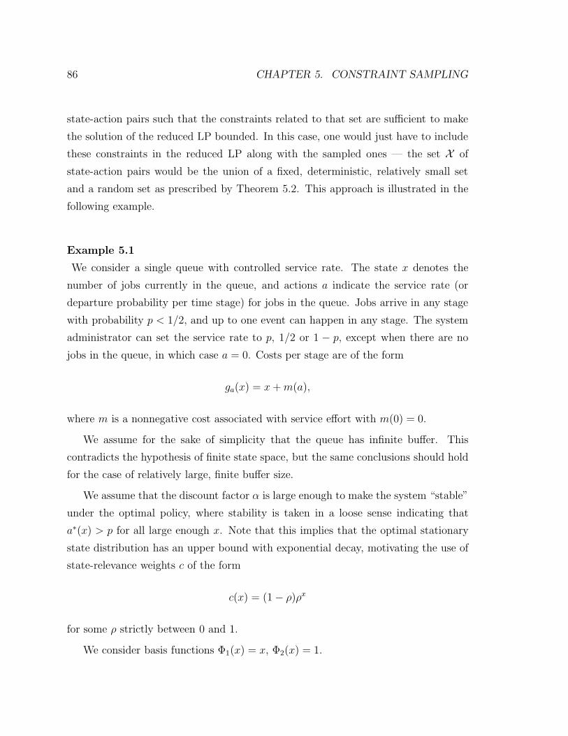
86 CHAPTER 5. CONSTRAINT SAMPLING
state-action pairs such that the constraints related to that set are sufficient to make
the solution of the reduced LP bounded. In this case, one would just have to include
these constraints in the reduced LP along with the sampled ones — the set X of
state-action pairs would be the union of a fixed, deterministic, relatively small set
and a random set as prescribed by Theorem 5.2. This approach is illustrated in the
following example.
Example 5.1
We consider a single queue with controlled service rate. The state x denotes the
number of jobs currently in the queue, and actions a indicate the service rate (or
departure probability per time stage) for jobs in the queue. Jobs arrive in any stage
with probability p < 1/2, and up to one event can happen in any stage. The system
administrator can set the service rate to p, 1/2 or 1 − p, except when there are no
jobs in the queue, in which case a = 0. Costs per stage are of the form
ga(x) = x+m(a),
where m is a nonnegative cost associated with service effort with m(0) = 0.
We assume for the sake of simplicity that the queue has infinite buffer. This
contradicts the hypothesis of finite state space, but the same conclusions should hold
for the case of relatively large, finite buffer size.
We assume that the discount factor α is large enough to make the system “stable”
under the optimal policy, where stability is taken in a loose sense indicating that
a∗(x) > p for all large enough x. Note that this implies that the optimal stationary
state distribution has an upper bound with exponential decay, motivating the use of
state-relevance weights c of the form
c(x) = (1− ρ)ρx
for some ρ strictly between 0 and 1.
We consider basis functions Φ1(x) = x, Φ2(x) = 1.
5.3. HIGH-CONFIDENCE SAMPLING AND ALP 87
1+m(1-p)
0
0
1-αpαp[1+m(1-p)](1-αp)(1-α)
,( )
(1-ρ)[1+m(1-p)](1-ρ)(1-αp)-ρ(1-α) (1- )(1-αp)-ρ(1-α)
ρρ[1+m(1-p)] ),( -
r1
r2
c'Φr 0>
(T Φr)(0)u' r)(0)> Φ
(T u' Φr)(1) > Φr)(1)
Figure 5.3: Typical feasible region for Example 5.1, constraints (5.27)-(5.29), with0 < ρ < 1, α ≈ 1, p < 1/2(graph constructed with ρ = 0.9, α = 0.99, p = 0.4,m(0) = 0, m(1− p) = 1).
Now consider the constraints
−αpr1 + (1− α)r2 ≤ 0 (5.27)
(1− 2αp)r1 + (1− α)r2 ≤ 1 +m(1− p) (5.28)
ρr1 + (1− ρ)r2 ≥ 0 (5.29)
The first and second constraints correspond to state-action pairs (0, 0) and (1, 1− p).The third one is equivalent to cT Φr ≥ 0. This constraint is automatically satisfied
by any optimal solution of the reduced LP, since all costs are nonnegative, implying
that r = 0 is always a feasible solution. The feasible region of (5.27)-(5.29) is shown
in Figure 5.3. It is seen to be bounded with maximum values of |ri| of the order of
1/(1 − α). Therefore Φr must be bounded in norm for any reduced LP including
(5.27) and (5.28), and one expects Mu∗,p to be O(1/(1− α)).
Finally, we mention a third possibility, which renders the bounded reduced LP a
88 CHAPTER 5. CONSTRAINT SAMPLING
problem of convex optimization rather than an LP. This involves adding the constraint
‖Φr‖1,c ≤ 2‖Ju‖1,c, (5.30)
for an arbitrarily chosen policy u. This constraint implies constraint (5.24) on the
norm of solutions of the approximate LP, therefore it is satisfied by optimal solutions
of the approximate LP. It should make Mu∗,p proportional to ‖Ju‖1,c, at least for small
p > 1. A potential advantage of this approach is that in some cases it may be easier to
estimate ‖Ju‖1,c than to find a small set of constraints to ensure boundedness in the
reduced LP. However, it requires devising a way of dealing with constraint (5.30) when
solving the bounded reduced LP. This might not be an easy task, considering this
constraint involves computation of L1 norms (i.e., summations) in a high-dimensional
space.
5.3.2 Choosing the Constraint Sampling Distribution
In Theorem 5.2, we assume that states are sampled according to distribution µu∗ for
some optimal policy u∗. We will generally not be able to compute µu∗ in practice, as
we do not know any optimal policy u∗; we have to sample constraints according to
an alternative distribution µ. This affects the error bound (5.14) through the term
‖1(Φr)(·)−(Tu∗ )(Φr)(·)>0‖ p−1p
,µu∗, (5.31)
which can no longer be shown to be less than or equal to (1−α)ε6
. Instead, we have
‖1(Φr)(·)−(Tu∗ )(Φr)(·)>0‖ p−1p
,µ ≤(1− α)ε
6.
The problem of ensuring that (5.31) is small given that constraints are sampled ac-
cording to µ corresponds to a problem of UCEP in which the sampling distribution
and the testing distributions differ. Intuitively, we expect that if µ is reasonably close
to µu∗ , (5.31) should remain relatively small.
How to choose µ is still an open question. As a simple heuristic, noting that
5.3. HIGH-CONFIDENCE SAMPLING AND ALP 89
µ∗(x) → c(x) as α → 0, one might choose µ = c. This is the approach taken in the
case studies presented in Chapter 6. This choice is also justified by the realization
that in many applications c would be the best estimate for πu∗ that can be obtained,
and if it were correct, we would have µu∗ = c = πµ∗ .
5.3.3 Dealing with Large Action Spaces
Generating approximations to the optimal value function within an approximation
architecture aims to alleviate the problems arising when one deals with large state
spaces. If the action space is also large, additional difficulties may be encountered;
in the specific case of approximate linear programming, the number of constraints
involved in the reduced LP becomes intractable as the cardinality of the action sets
Ax increases. In particular, our bound (5.13) on the number of sampled constraints
grows polynomially in A, the cardinality of the largest action set.
Complexity in the action space can be exchanged for complexity in the state space
by breaking each action under consideration into a sequence of actions taking values
in smaller sets [5]. Specifically, given an alphabet with S symbols — assume for
simplicity the symbols are 0,1,...,S-1 — and a finite set of actions Ax of cardinality
less than or equal to A, actions in this set can be mapped to words of length at most
dlogS Ae. Hence we can change the decision on an action a ∈ Ax into a decision on a
sequence of dlogS Ae symbols.
We define a new MDP as follows:
• States x are given by a tuple (x, x, i), interpreted as follows: x ∈ S represents
the state in the original MDP; x ∈ {0, 1, . . . , S−1}dlogS Ae represents an encoding
of an action in Ax being taken; i ∈ {1, 2, . . . , dlogS Ae} represents which entry
in vector a we will decide upon next.
• There are S actions associated with each state (x, x, i), corresponding to setting
xi to 0, 1, . . . S − 1.
• Taking action “set xi to v” causes a deterministic transition from x to x+, where
x+j = x+
j for j 6= i and x+i = v. The system transitions from state (x, xa, i) to
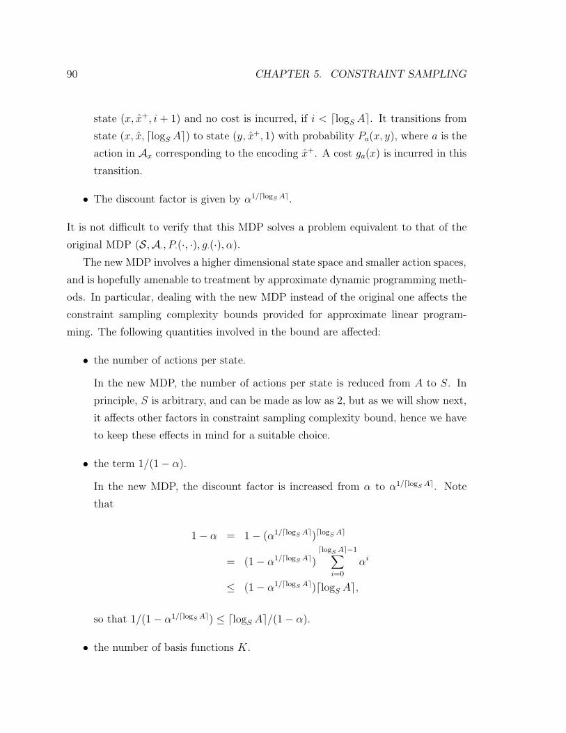
90 CHAPTER 5. CONSTRAINT SAMPLING
state (x, x+, i + 1) and no cost is incurred, if i < dlogS Ae. It transitions from
state (x, x, dlogS Ae) to state (y, x+, 1) with probability Pa(x, y), where a is the
action in Ax corresponding to the encoding x+. A cost ga(x) is incurred in this
transition.
• The discount factor is given by α1/dlogS Ae.
It is not difficult to verify that this MDP solves a problem equivalent to that of the
original MDP (S,A·, P·(·, ·), g·(·), α).
The new MDP involves a higher dimensional state space and smaller action spaces,
and is hopefully amenable to treatment by approximate dynamic programming meth-
ods. In particular, dealing with the new MDP instead of the original one affects the
constraint sampling complexity bounds provided for approximate linear program-
ming. The following quantities involved in the bound are affected:
• the number of actions per state.
In the new MDP, the number of actions per state is reduced from A to S. In
principle, S is arbitrary, and can be made as low as 2, but as we will show next,
it affects other factors in constraint sampling complexity bound, hence we have
to keep these effects in mind for a suitable choice.
• the term 1/(1− α).
In the new MDP, the discount factor is increased from α to α1/dlogS Ae. Note
that
1− α = 1− (α1/dlogS Ae)dlogS Ae
= (1− α1/dlogS Ae)dlogS Ae−1∑
i=0
αi
≤ (1− α1/dlogS Ae)dlogS Ae,
so that 1/(1− α1/dlogS Ae) ≤ dlogS Ae/(1− α).
• the number of basis functions K.
5.4. CLOSING REMARKS 91
In the new MDP, we have a higher dimensional state space, hence we may need a
larger number of basis functions in order to achieve an acceptable approximation
to the optimal value function. The actual increase on the number of basis
functions will depend on the structure of the problem at hand.
The bound on the number of constraints being sampled is polynomial in the three
terms above. Hence implementation of the reduced LP for the modified version of an
MDP will require a number of constraints polynomial in S and in dlogS Ae, contrasted
with the number of constraints necessary for the original MDP, which is polynomial
in A. However, the original complexity of the action space is transformed into extra
complexity in the state space, which may incur extra difficulties in the selection of
basis functions. Note the number of constraints is also polynomial in the number of
basis functions. Nevertheless, there is a potential advantage of using the new MDP,
as it provides an opportunity for structures associate with the action space to be
exploited in the same way as structures associated with the state space are.
5.4 Closing Remarks
In this chapter, we have analyzed a constraint sampling algorithm as an approxima-
tion method for dealing with the large number of constraints involved in the approxi-
mate LP. We have shown how near-feasibility can be ensured by sampling a tractable
number of constraints and established bounds on the error that near-feasibility in-
troduces in the optimal value function approximation. The error bounds show that,
under moderate assumptions, the approximation to the optimal value function yielded
by the reduced LP has error comparable to the error resulting from the approximate
LP. They also provide an ideal constraint sampling distribution, which can serve as
a guide in the sampling process even though it cannot be calculated.
An important observation is that the bounds on the number of samples necessary
to ensure near-feasibility are loose. Indeed, they only exploit the fact that constraints
live in a low-dimensional space; efficiency of the constraint sampling scheme is then
enabled by the fact that after a certain number of constraints is sampled, any other
constraint will most likely be close to one of the already sampled constraints. Hence
92 CHAPTER 5. CONSTRAINT SAMPLING
we do not exploit any possible regularity associated with the structure of the con-
straints, or a particular choice of basis functions, which might lead to much tighter
bounds or even exact solution of the approximate LP. The latter approach can be
found in the literature. Morrison and Kumar [39] formulate approximate linear pro-
gramming algorithms for queueing problems with a certain choice of basis functions
that renders all but a relatively small, tractable number of constraints provably re-
dundant. Guestrin et al. [24] exploit the structure present in factored MDP’s to
efficiently implement approximate linear programming with an exponentially lower
number of constraints. Schuurmans and Patrascu [42] devise a constraint generation
scheme for factored MDP’s which, although it lacks the guarantees of the algorithm
presented in [24] (the worst case is still exponential), requires a smaller amount of
time on average. Grotschel [23] presents an efficient cutting-plane method for the
traveling salesman problem.
Exploitation of particular properties and regularities of the problem at hand is
obviously useful and the constraint sampling scheme is not meant as a substitute for
that; the main contribution of this chapter is to show that, even if such regularities
are not known or do not exist in a given problem, variants of approximate linear
programming can still be implemented efficiently.
There are several ways in which the present results can be extended, and we men-
tion a few. It may be possible to improve the constant and exponential terms in the
bounds on the number of constraints needed for near-feasibility; our main focus was
on establishing that the number of constraints is tractable, rather than on derivation
of the tightest possible bounds. The problem of sampling constraints according to
one distribution but measuring errors according to another one, described in Section
5.3.2, pertains not only to approximate linear programming but to the UCEP theory
in general, and is discussed in [57], but still remains an open question. With the
impossibility of computing the stationary distribution associated with optimal poli-
cies, there is a question whether one may use an adaptive scheme to choose sampling
distributions according to policies being generated in intermediate steps. Finally, the
ideas on how to generate the bounded reduced LP presented here require further
investigation.
Chapter 6
Case Studies
In this chapter, we present applications of approximate linear programming to queue-
ing problems and web server farm management. The applications illustrate some prac-
tical aspects in the implementation of approximate linear programming and demon-
strate its competitiveness relative to other algorithms for tackling the problems being
considered.
6.1 Queueing Problems
We start with three queueing problems, with increasing state space dimensions. In
all examples, we assume that at most one event (arrival/departure) occurs at each
time step. The first example, involving a single queue, illustrates how state-relevance
weights influence the solution of the approximate LP, testing the ideas presented
in Chapter 3 against a larger and more realistic problem. The next two examples
involve higher dimensional state spaces and demonstrate the performance of approxi-
mate linear programming as compared to other heuristics commonly used in queueing
problems.
93
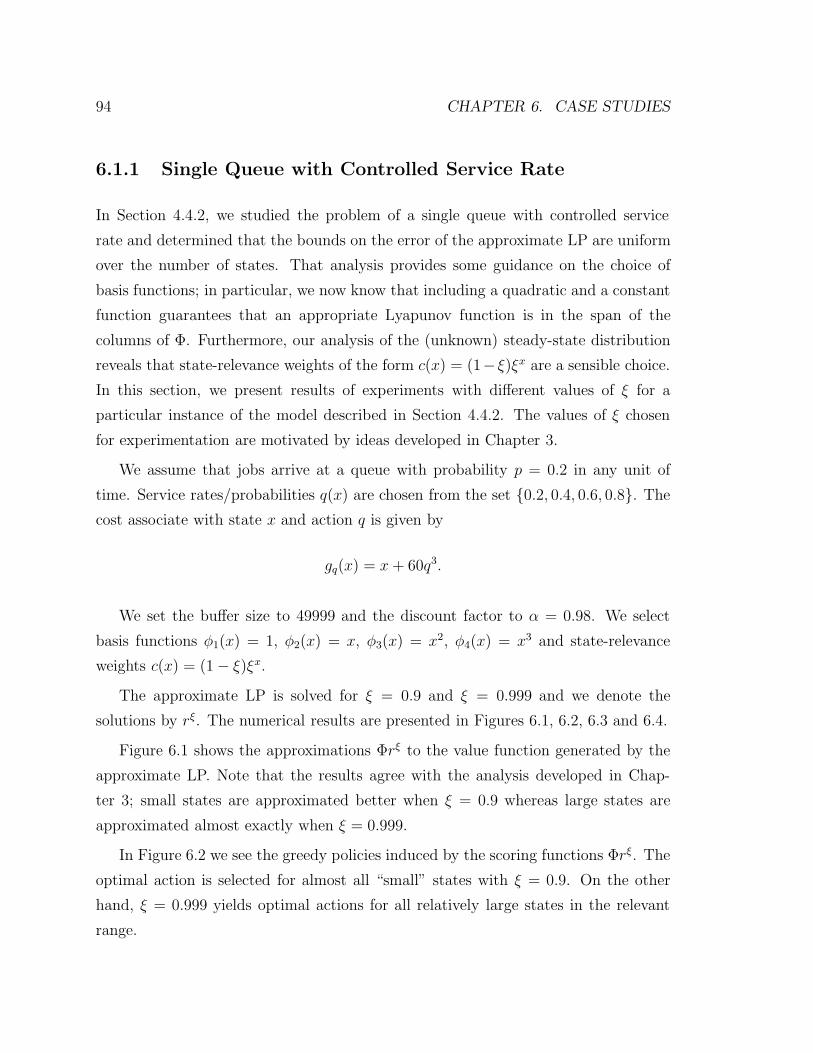
94 CHAPTER 6. CASE STUDIES
6.1.1 Single Queue with Controlled Service Rate
In Section 4.4.2, we studied the problem of a single queue with controlled service
rate and determined that the bounds on the error of the approximate LP are uniform
over the number of states. That analysis provides some guidance on the choice of
basis functions; in particular, we now know that including a quadratic and a constant
function guarantees that an appropriate Lyapunov function is in the span of the
columns of Φ. Furthermore, our analysis of the (unknown) steady-state distribution
reveals that state-relevance weights of the form c(x) = (1− ξ)ξx are a sensible choice.
In this section, we present results of experiments with different values of ξ for a
particular instance of the model described in Section 4.4.2. The values of ξ chosen
for experimentation are motivated by ideas developed in Chapter 3.
We assume that jobs arrive at a queue with probability p = 0.2 in any unit of
time. Service rates/probabilities q(x) are chosen from the set {0.2, 0.4, 0.6, 0.8}. The
cost associate with state x and action q is given by
gq(x) = x+ 60q3.
We set the buffer size to 49999 and the discount factor to α = 0.98. We select
basis functions φ1(x) = 1, φ2(x) = x, φ3(x) = x2, φ4(x) = x3 and state-relevance
weights c(x) = (1− ξ)ξx.
The approximate LP is solved for ξ = 0.9 and ξ = 0.999 and we denote the
solutions by rξ. The numerical results are presented in Figures 6.1, 6.2, 6.3 and 6.4.
Figure 6.1 shows the approximations Φrξ to the value function generated by the
approximate LP. Note that the results agree with the analysis developed in Chap-
ter 3; small states are approximated better when ξ = 0.9 whereas large states are
approximated almost exactly when ξ = 0.999.
In Figure 6.2 we see the greedy policies induced by the scoring functions Φrξ. The
optimal action is selected for almost all “small” states with ξ = 0.9. On the other
hand, ξ = 0.999 yields optimal actions for all relatively large states in the relevant
range.
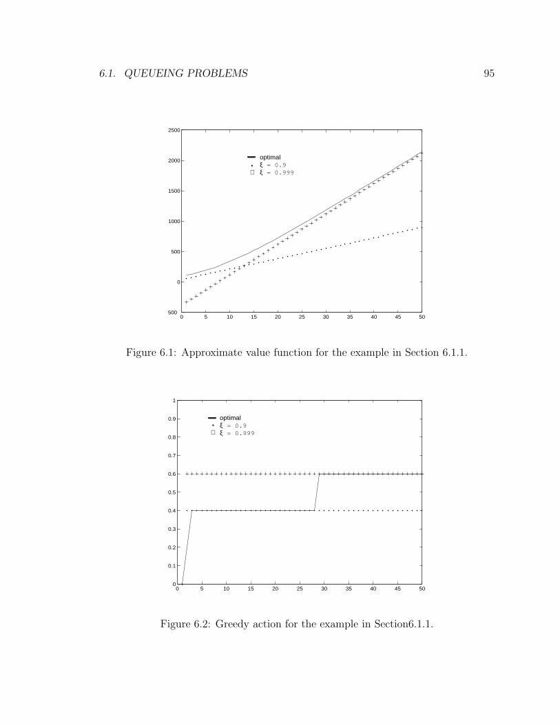
6.1. QUEUEING PROBLEMS 95
0 5 10 15 20 25 30 35 40 45 50500
0
500
1000
1500
2000
2500
optimalξ = 0.9ξ = 0.999+
.
Figure 6.1: Approximate value function for the example in Section 6.1.1.
0 5 10 15 20 25 30 35 40 45 500
0.1
0.2
0.3
0.4
0.5
0.6
0.7
0.8
0.9
1
optimalξ = 0.9ξ = 0.999
.+
Figure 6.2: Greedy action for the example in Section6.1.1.
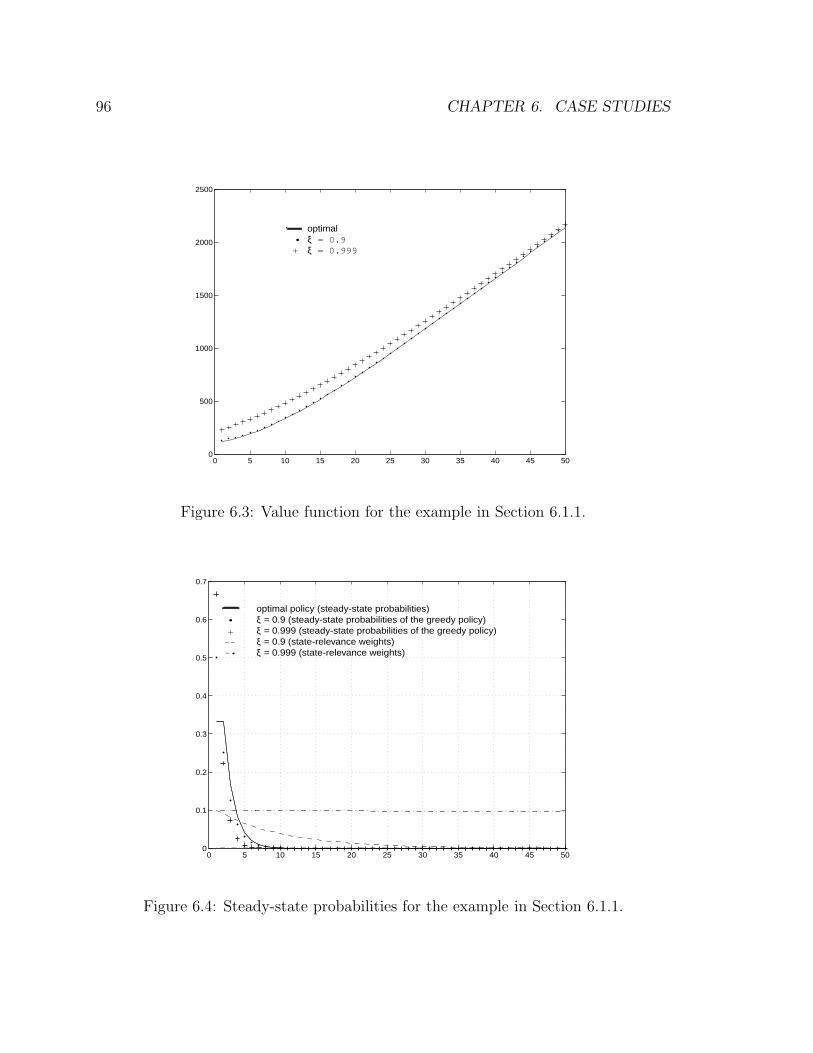
96 CHAPTER 6. CASE STUDIES
0 5 10 15 20 25 30 35 40 45 500
500
1000
1500
2000
2500
optimalξ = 0.9ξ = 0.999
.+
Figure 6.3: Value function for the example in Section 6.1.1.
0 5 10 15 20 25 30 35 40 45 500
0.1
0.2
0.3
0.4
0.5
0.6
0.7
optimal policy (steady-state probabilities)ξ = 0.9 (steady-state probabilities of the greedy policy)ξ = 0.999 (steady-state probabilities of the greedy policy) ξ = 0.9 (state-relevance weights)ξ = 0.999 (state-relevance weights)
.+---.
Figure 6.4: Steady-state probabilities for the example in Section 6.1.1.
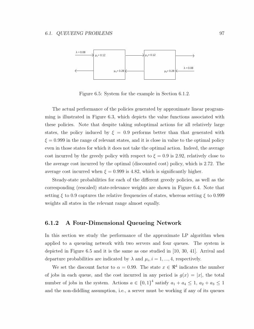
6.1. QUEUEING PROBLEMS 97
= 0.12µ1 = 0.12µ
= 0.28µ= 0.28µ4 3
2
λ = 0.08
λ = 0.08
Figure 6.5: System for the example in Section 6.1.2.
The actual performance of the policies generated by approximate linear program-
ming is illustrated in Figure 6.3, which depicts the value functions associated with
these policies. Note that despite taking suboptimal actions for all relatively large
states, the policy induced by ξ = 0.9 performs better than that generated with
ξ = 0.999 in the range of relevant states, and it is close in value to the optimal policy
even in those states for which it does not take the optimal action. Indeed, the average
cost incurred by the greedy policy with respect to ξ = 0.9 is 2.92, relatively close to
the average cost incurred by the optimal (discounted cost) policy, which is 2.72. The
average cost incurred when ξ = 0.999 is 4.82, which is significantly higher.
Steady-state probabilities for each of the different greedy policies, as well as the
corresponding (rescaled) state-relevance weights are shown in Figure 6.4. Note that
setting ξ to 0.9 captures the relative frequencies of states, whereas setting ξ to 0.999
weights all states in the relevant range almost equally.
6.1.2 A Four-Dimensional Queueing Network
In this section we study the performance of the approximate LP algorithm when
applied to a queueing network with two servers and four queues. The system is
depicted in Figure 6.5 and it is the same as one studied in [10, 30, 41]. Arrival and
departure probabilities are indicated by λ and µi, i = 1, ..., 4, respectively.
We set the discount factor to α = 0.99. The state x ∈ <4 indicates the number
of jobs in each queue, and the cost incurred in any period is g(x) = |x|, the total
number of jobs in the system. Actions a ∈ {0, 1}4 satisfy a1 + a4 ≤ 1, a2 + a3 ≤ 1
and the non-diddling assumption, i.e., a server must be working if any of its queues
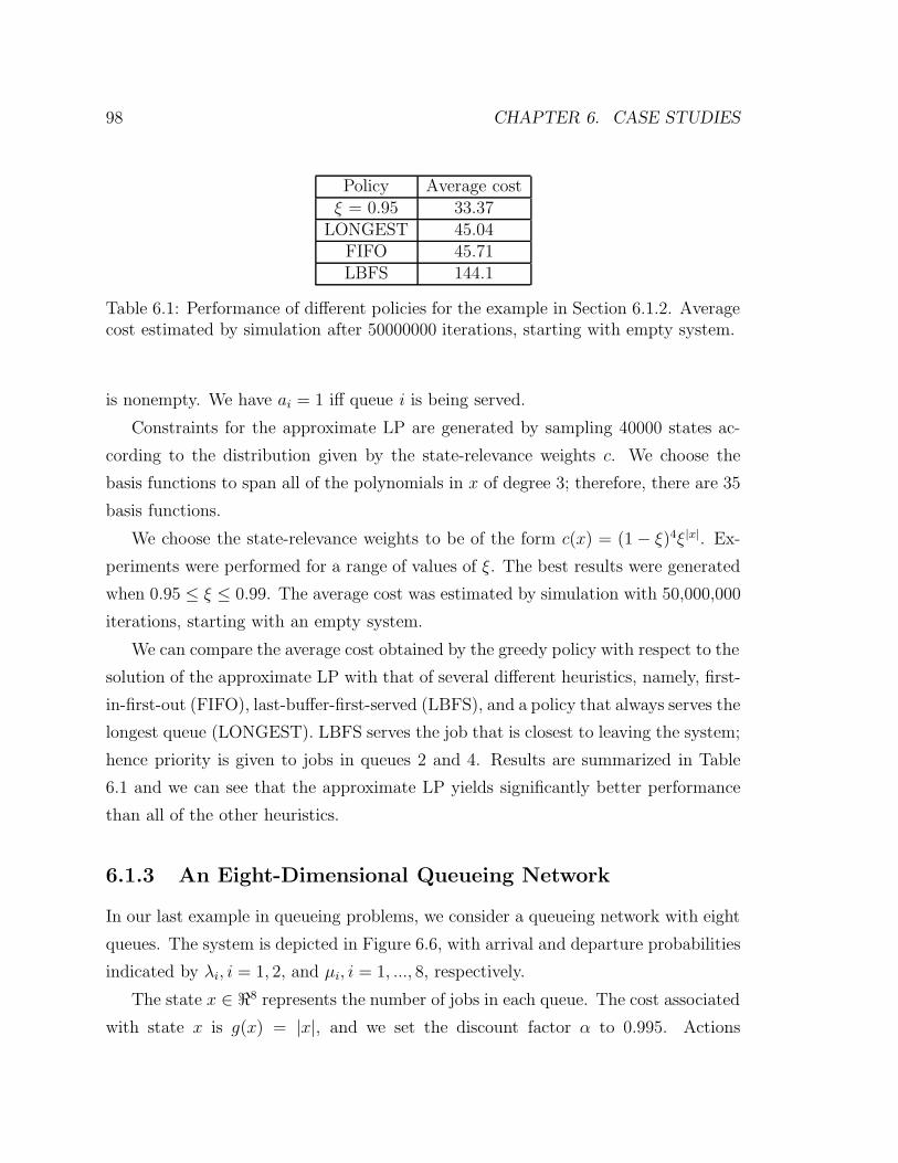
98 CHAPTER 6. CASE STUDIES
Policy Average costξ = 0.95 33.37
LONGEST 45.04FIFO 45.71LBFS 144.1
Table 6.1: Performance of different policies for the example in Section 6.1.2. Averagecost estimated by simulation after 50000000 iterations, starting with empty system.
is nonempty. We have ai = 1 iff queue i is being served.
Constraints for the approximate LP are generated by sampling 40000 states ac-
cording to the distribution given by the state-relevance weights c. We choose the
basis functions to span all of the polynomials in x of degree 3; therefore, there are 35
basis functions.
We choose the state-relevance weights to be of the form c(x) = (1 − ξ)4ξ|x|. Ex-
periments were performed for a range of values of ξ. The best results were generated
when 0.95 ≤ ξ ≤ 0.99. The average cost was estimated by simulation with 50,000,000
iterations, starting with an empty system.
We can compare the average cost obtained by the greedy policy with respect to the
solution of the approximate LP with that of several different heuristics, namely, first-
in-first-out (FIFO), last-buffer-first-served (LBFS), and a policy that always serves the
longest queue (LONGEST). LBFS serves the job that is closest to leaving the system;
hence priority is given to jobs in queues 2 and 4. Results are summarized in Table
6.1 and we can see that the approximate LP yields significantly better performance
than all of the other heuristics.
6.1.3 An Eight-Dimensional Queueing Network
In our last example in queueing problems, we consider a queueing network with eight
queues. The system is depicted in Figure 6.6, with arrival and departure probabilities
indicated by λi, i = 1, 2, and µi, i = 1, ..., 8, respectively.
The state x ∈ <8 represents the number of jobs in each queue. The cost associated
with state x is g(x) = |x|, and we set the discount factor α to 0.995. Actions
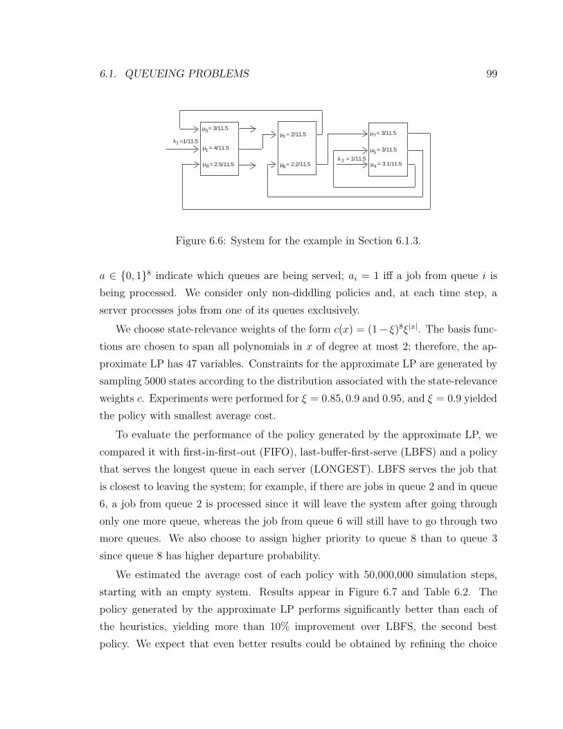
6.1. QUEUEING PROBLEMS 99
=1/11.5λ1
= 1/11.5λ 2
= 4/11.5µ1
= 2.5/11.5µ8
= 3/11.5µ3= 2/11.5µ2
= 2.2/11.5µ6 = 3.1/11.5µ4
= 3/11.5µ5
= 3/11.5µ7
Figure 6.6: System for the example in Section 6.1.3.
a ∈ {0, 1}8 indicate which queues are being served; ai = 1 iff a job from queue i is
being processed. We consider only non-diddling policies and, at each time step, a
server processes jobs from one of its queues exclusively.
We choose state-relevance weights of the form c(x) = (1− ξ)8ξ|x|. The basis func-
tions are chosen to span all polynomials in x of degree at most 2; therefore, the ap-
proximate LP has 47 variables. Constraints for the approximate LP are generated by
sampling 5000 states according to the distribution associated with the state-relevance
weights c. Experiments were performed for ξ = 0.85, 0.9 and 0.95, and ξ = 0.9 yielded
the policy with smallest average cost.
To evaluate the performance of the policy generated by the approximate LP, we
compared it with first-in-first-out (FIFO), last-buffer-first-serve (LBFS) and a policy
that serves the longest queue in each server (LONGEST). LBFS serves the job that
is closest to leaving the system; for example, if there are jobs in queue 2 and in queue
6, a job from queue 2 is processed since it will leave the system after going through
only one more queue, whereas the job from queue 6 will still have to go through two
more queues. We also choose to assign higher priority to queue 8 than to queue 3
since queue 8 has higher departure probability.
We estimated the average cost of each policy with 50,000,000 simulation steps,
starting with an empty system. Results appear in Figure 6.7 and Table 6.2. The
policy generated by the approximate LP performs significantly better than each of
the heuristics, yielding more than 10% improvement over LBFS, the second best
policy. We expect that even better results could be obtained by refining the choice
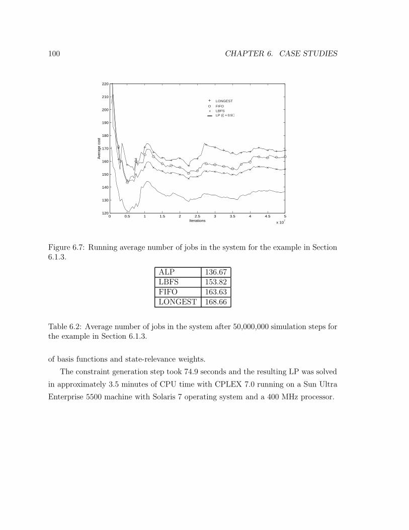
100 CHAPTER 6. CASE STUDIES
0 0.5 1 1.5 2 2.5 3 3.5 4 4.5 5
x 107
120
130
140
150
160
170
180
190
200
210
220
Ave
rage
cos
t
Iterations
+ OX
LONGEST
FIFOLBFSLP (ξ = 0.9)
Figure 6.7: Running average number of jobs in the system for the example in Section6.1.3.
ALP 136.67LBFS 153.82FIFO 163.63LONGEST 168.66
Table 6.2: Average number of jobs in the system after 50,000,000 simulation steps forthe example in Section 6.1.3.
of basis functions and state-relevance weights.
The constraint generation step took 74.9 seconds and the resulting LP was solved
in approximately 3.5 minutes of CPU time with CPLEX 7.0 running on a Sun Ultra
Enterprise 5500 machine with Solaris 7 operating system and a 400 MHz processor.

6.2. WEB SERVER FARM MANAGEMENT 101
6.2 Web Server Farm Management
As Internet-based transactions become an increasingly important part of business,
we observe a drift from relatively amateurish web site management to outsourcing
of this kind of activity to companies providing information technology services. The
benefits of outsourcing web site management are clear: first, businesses can rely
on core competencies of information technology companies and are free to focus on
their main activities; second, information technology companies having contracts with
multiple web sites have the opportunity to leverage economies of scale.
The development of this new kind of service brings about a host of challenging
issues. A large part of the incentive to outsourcing web site management is that
specialized information technology companies may be able to provide better quality
of service to web site users. Hence various questions arise: What kinds of guarantees
can the web site hosting service provider guarantee? What is desirable and acceptable
from the web site standpoint? How should different service-level guarantees be priced?
Besides questions on how contracts should be made, the web site hosting service
provider must also face a number of questions on how to manage resources in their
physical systems. Optimal resource utilization reduces costs and allows for better
quality of service; furthermore, it leads to a more precise assessment of how meeting
different service-level guarantees maps to use of resources. One might expect that
much insight on the contract-level questions of how to price services and how to
design service-level guarantees could be gained in the process of understanding how
to best utilize physical resources.
Our focus in this section is on resource allocation problems. We assume that the
web site hosting service provider has contracts with multiple web sites and maintains a
collection of servers — a web server farm — to process requests for pages in these web
sites. We consider the problems of allocation of servers to web sites, and scheduling
and routing of requests for each distinct web site.
In the next section, we provide a general description of the resource allocation
problems. We show how there is a natural division between the problem of server
allocation and the problem of scheduling and routing, due to differences in time scales
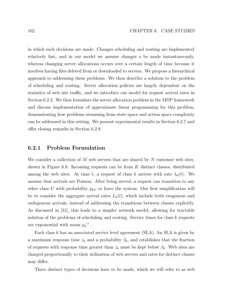
102 CHAPTER 6. CASE STUDIES
in which such decisions are made. Changes scheduling and routing are implemented
relatively fast, and in our model we assume changes o be made instantaneously,
whereas changing server allocations occurs over a certain length of time because it
involves having files deleted from or downloaded to servers. We propose a hierarchical
approach to addressing these problems. We then describe a solution to the problem
of scheduling and routing. Server allocation policies are largely dependent on the
statistics of web site traffic, and we introduce our model for request arrival rates in
Section 6.2.3. We then formulate the server allocation problem in the MDP framework
and discuss implementation of approximate linear programming for this problem,
demonstrating how problems stemming from state space and action space complexity
can be addressed in this setting. We present experimental results in Section 6.2.7 and
offer closing remarks in Section 6.2.8.
6.2.1 Problem Formulation
We consider a collection of M web servers that are shared by N customer web sites,
shown in Figure 6.8. Incoming requests can be from K distinct classes, distributed
among the web sites. At time t, a request of class k arrives with rate λk(t). We
assume that arrivals are Poisson. After being served, a request can transition to any
other class k′ with probability pkk′ or leave the system. Our first simplification will
be to consider the aggregate arrival rates Lk(t), which include both exogenous and
endogenous arrivals, instead of addressing the transitions between classes explicitly.
As discussed in [31], this leads to a simpler network model, allowing for tractable
solution of the problems of scheduling and routing. Service times for class k requests
are exponential with mean µ−1k .
Each class k has an associated service level agreement (SLA). An SLA is given by
a maximum response time zk and a probability βk, and establishes that the fraction
of requests with response time greater than zk must be kept below βk. Web sites are
charged proportionally to their utilization of web servers and rates for distinct classes
may differ.
Three distinct types of decisions have to be made, which we will refer to as web
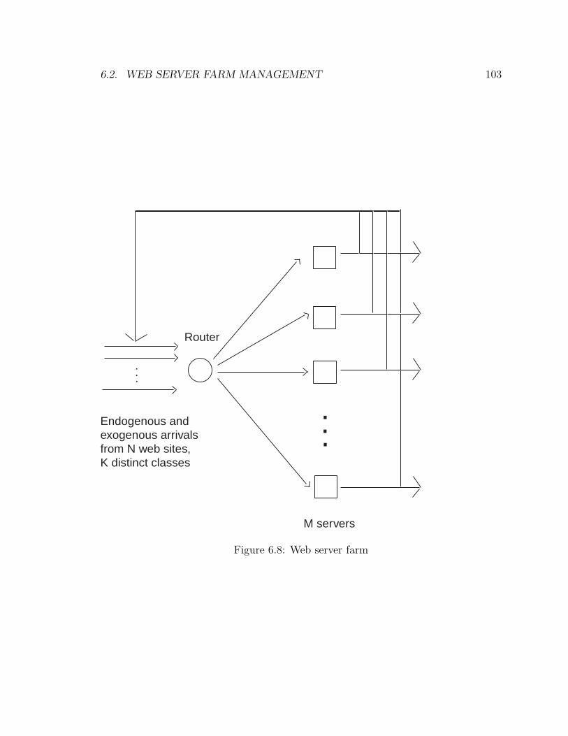
6.2. WEB SERVER FARM MANAGEMENT 103
...
...
Endogenous andexogenous arrivals from N web sites,K distinct classes
M servers
Router
Figure 6.8: Web server farm
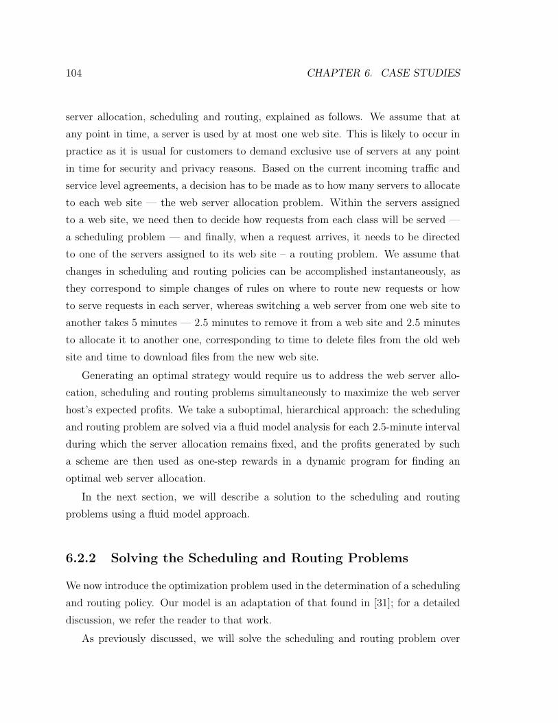
104 CHAPTER 6. CASE STUDIES
server allocation, scheduling and routing, explained as follows. We assume that at
any point in time, a server is used by at most one web site. This is likely to occur in
practice as it is usual for customers to demand exclusive use of servers at any point
in time for security and privacy reasons. Based on the current incoming traffic and
service level agreements, a decision has to be made as to how many servers to allocate
to each web site — the web server allocation problem. Within the servers assigned
to a web site, we need then to decide how requests from each class will be served —
a scheduling problem — and finally, when a request arrives, it needs to be directed
to one of the servers assigned to its web site – a routing problem. We assume that
changes in scheduling and routing policies can be accomplished instantaneously, as
they correspond to simple changes of rules on where to route new requests or how
to serve requests in each server, whereas switching a web server from one web site to
another takes 5 minutes — 2.5 minutes to remove it from a web site and 2.5 minutes
to allocate it to another one, corresponding to time to delete files from the old web
site and time to download files from the new web site.
Generating an optimal strategy would require us to address the web server allo-
cation, scheduling and routing problems simultaneously to maximize the web server
host’s expected profits. We take a suboptimal, hierarchical approach: the scheduling
and routing problem are solved via a fluid model analysis for each 2.5-minute interval
during which the server allocation remains fixed, and the profits generated by such
a scheme are then used as one-step rewards in a dynamic program for finding an
optimal web server allocation.
In the next section, we will describe a solution to the scheduling and routing
problems using a fluid model approach.
6.2.2 Solving the Scheduling and Routing Problems
We now introduce the optimization problem used in the determination of a scheduling
and routing policy. Our model is an adaptation of that found in [31]; for a detailed
discussion, we refer the reader to that work.
As previously discussed, we will solve the scheduling and routing problem over
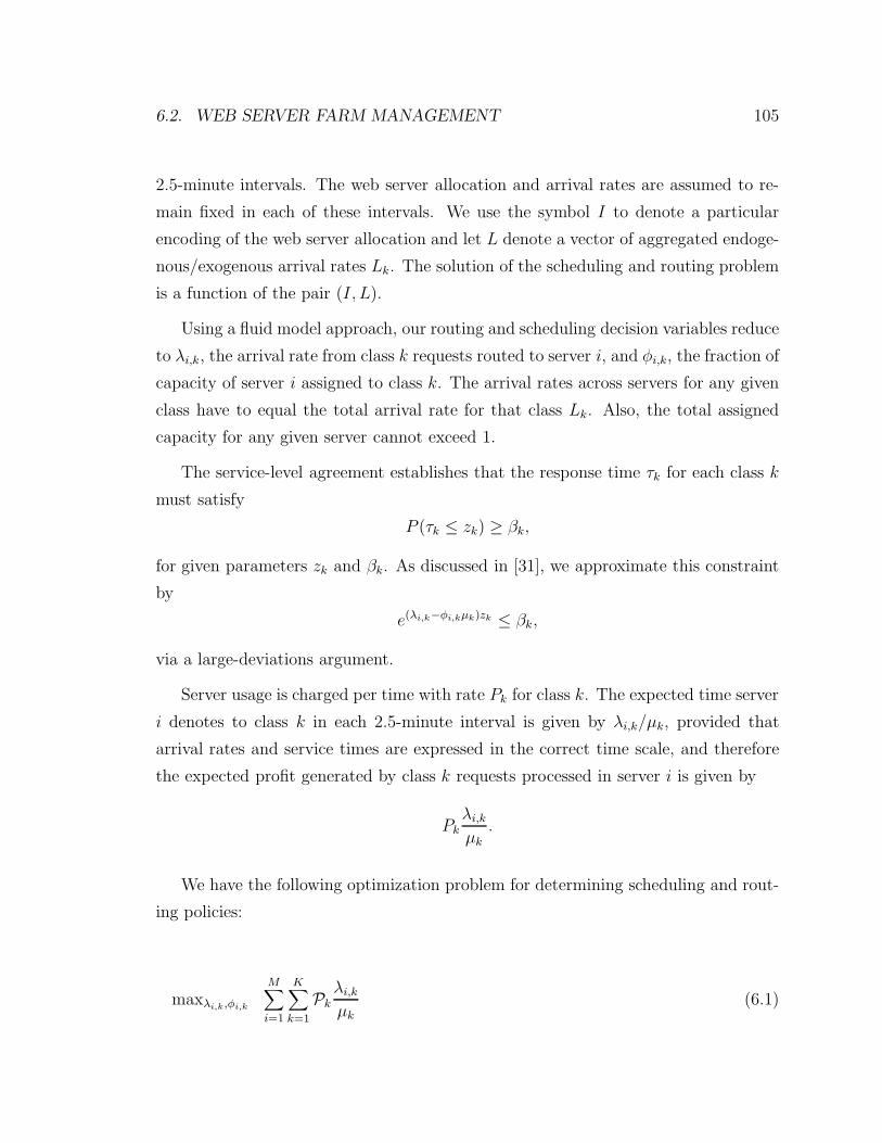
6.2. WEB SERVER FARM MANAGEMENT 105
2.5-minute intervals. The web server allocation and arrival rates are assumed to re-
main fixed in each of these intervals. We use the symbol I to denote a particular
encoding of the web server allocation and let L denote a vector of aggregated endoge-
nous/exogenous arrival rates Lk. The solution of the scheduling and routing problem
is a function of the pair (I, L).
Using a fluid model approach, our routing and scheduling decision variables reduce
to λi,k, the arrival rate from class k requests routed to server i, and φi,k, the fraction of
capacity of server i assigned to class k. The arrival rates across servers for any given
class have to equal the total arrival rate for that class Lk. Also, the total assigned
capacity for any given server cannot exceed 1.
The service-level agreement establishes that the response time τk for each class k
must satisfy
P (τk ≤ zk) ≥ βk,
for given parameters zk and βk. As discussed in [31], we approximate this constraint
by
e(λi,k−φi,kµk)zk ≤ βk,
via a large-deviations argument.
Server usage is charged per time with rate Pk for class k. The expected time server
i denotes to class k in each 2.5-minute interval is given by λi,k/µk, provided that
arrival rates and service times are expressed in the correct time scale, and therefore
the expected profit generated by class k requests processed in server i is given by
Pkλi,k
µk.
We have the following optimization problem for determining scheduling and rout-
ing policies:
maxλi,k,φi,k
M∑i=1
K∑k=1
Pkλi,k
µk(6.1)
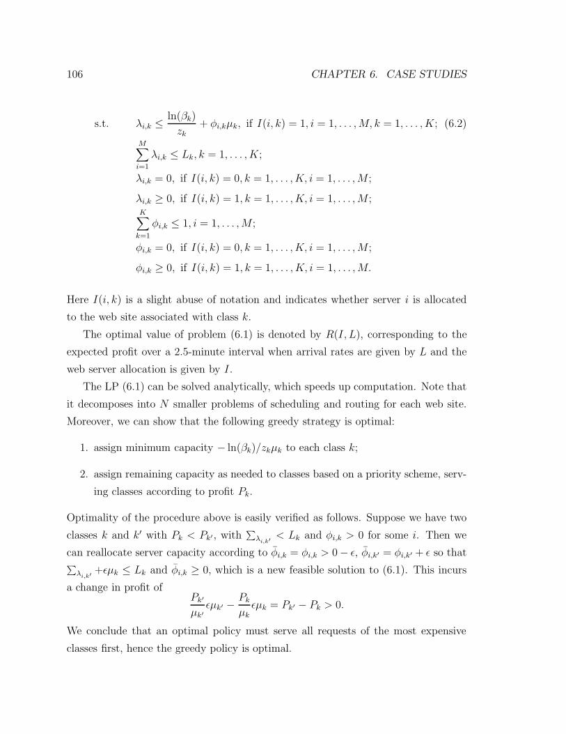
106 CHAPTER 6. CASE STUDIES
s.t. λi,k ≤ ln(βk)
zk+ φi,kµk, if I(i, k) = 1, i = 1, . . . ,M, k = 1, . . . , K; (6.2)
M∑i=1
λi,k ≤ Lk, k = 1, . . . , K;
λi,k = 0, if I(i, k) = 0, k = 1, . . . , K, i = 1, . . . ,M ;
λi,k ≥ 0, if I(i, k) = 1, k = 1, . . . , K, i = 1, . . . ,M ;K∑
k=1
φi,k ≤ 1, i = 1, . . . ,M ;
φi,k = 0, if I(i, k) = 0, k = 1, . . . , K, i = 1, . . . ,M ;
φi,k ≥ 0, if I(i, k) = 1, k = 1, . . . , K, i = 1, . . . ,M.
Here I(i, k) is a slight abuse of notation and indicates whether server i is allocated
to the web site associated with class k.
The optimal value of problem (6.1) is denoted by R(I, L), corresponding to the
expected profit over a 2.5-minute interval when arrival rates are given by L and the
web server allocation is given by I.
The LP (6.1) can be solved analytically, which speeds up computation. Note that
it decomposes into N smaller problems of scheduling and routing for each web site.
Moreover, we can show that the following greedy strategy is optimal:
1. assign minimum capacity − ln(βk)/zkµk to each class k;
2. assign remaining capacity as needed to classes based on a priority scheme, serv-
ing classes according to profit Pk.
Optimality of the procedure above is easily verified as follows. Suppose we have two
classes k and k′ with Pk < Pk′, with∑
λi,k′ < Lk and φi,k > 0 for some i. Then we
can reallocate server capacity according to φi,k = φi,k > 0− ε, φi,k′ = φi,k′ + ε so that∑λi,k′ +εµk ≤ Lk and φi,k ≥ 0, which is a new feasible solution to (6.1). This incurs
a change in profit ofPk′
µk′εµk′ − Pk
µkεµk = Pk′ − Pk > 0.
We conclude that an optimal policy must serve all requests of the most expensive
classes first, hence the greedy policy is optimal.
6.2. WEB SERVER FARM MANAGEMENT 107
Note that constraint
λi,k ≤ ln(βk)
zk+ φi,kµk,
corresponding to the service-level agreement for class k, requires that a minimum
server capacity be to requests of class k even if that server is not processing any
requests of that type. This is due to the fact that the SLA constraint is based on
a large-deviation limit, which is not accurate for small (or zero) arrival rates λi,k.
Ideally, problem (6.1) would be reformulated to correct for that; however, that would
lead to a nonconvex optimization problem. In a different relaxation of the original
scheduling and routing problem, we may approximate the number of servers needed
for serving all requests of class k by
Lk
µk + ln(βk)zk
, (6.3)
and assign available servers to the classes associated with a web site according to that
number. In this situation, server capacity is not assigned to classes with no requests
being processed in a given server. Expression (6.3) is motivated by the fact that, if
a server i is totally dedicated to class k requests (φi,k = 1), it can process at most
µk + ln(βk)zk
requests of that type.
With expression (6.3) as an approximation for the number of servers needed for
each class, we have a nearly optimal policy by assigning available servers greedily
according to profit Pk/µk.
The web server allocation problem will be solved by dynamic programming. We
will use the optimal value of problem (6.1) — R(I,L) — as one-step rewards. Dynamic
programming is called for due to the time-variant nature of arrival rates: changes
in the incoming traffic will typically require adjustments in the number of servers
allocated to each web site. Before tackling the web server allocation problem, we will
discuss the arrival rate process.
108 CHAPTER 6. CASE STUDIES
6.2.3 The Arrival Rate Process
There are two types of web page requests in a web server farm: exogenous, corre-
sponding to users initiating a browsing session, and endogenous, corresponding to
subsequent requests in an already initiated session. As mentioned before, we will
consider the aggregated arrival rate, making no distinction between the two types of
requests.
We consider the following model for the arrival rate process for requests of class
k associated with web site i:
Lk(t+ 1) = max(Lk + ak(Lk(t)− Lk) + σkNk(t) +MkBi(t), 0). (6.4)
where {Nk(t), k = 1, . . . , K, t = 0, 1, . . .} is a collection of independent standard
normal random variables and {Bi(t), i = 1, . . . , N, t = 0, 1, . . .} is a collection of
independent Bernoulli variables.
We interpret the arrival rate process (6.4) as follows. Lk represents a prediction for
the average arrival rate associated with class k. We assume that arrival rates fluctuate
around their average value Lk, and ak is a scalar between 0 and 1 representing how
persistent deviations from the average arrival rate are. The normal random variables
Nk(t) represent regular fluctuations around the average arrival rate, and the Bernoulli
variables Bi(t) capture arrival bursts. Note that the occurrence of a burst is associated
with a web site as a whole, not with particular classes of users.
We now turn to the web server allocation problem, which is formulated in the
dynamic programming framework.
6.2.4 An MDP Model for the Web Server Allocation Prob-
lem
We model the web server allocation problem in discrete time, with each time step
corresponding to 2.5 minutes, corresponding to the time necessary to allocate or
deallocate a server.
6.2. WEB SERVER FARM MANAGEMENT 109
The state should contain all information that is important for the allocation deci-
sion. In the web server allocation problem, with the simplified model (6.4) for arrival
rates presented in Section 6.2.3, a natural choice for the state variable is the pair (I, L),
where I indicates the servers allocated to each web site and L is a K-dimensional
vector of arrival rates.
Actions A take values on the same space as web server configurations I and in-
dicate new web server configurations. Valid actions must satisfy the constraint that
only currently deallocated servers can be assigned to a web site.
A state (I, L) under action A transitions to state (A, L) with probability P (L, L)
determined by the arrival rate processes (6.4).
We have to specify rewards associated with each state-action pair. For simplicity,
we will assume that the arrival rate L remains constant over each time step in the
web server allocation problem, and consider the expected reward R(I, L) for the static
scheduling/routing decision given by the optimization problem (6.1).
We will seek to optimize the discounted infinite-horizon reward. We expect to use
reasonably large discount factors (in the experiments, α = 0.99) so that our criterion
can be viewed as an approximation to average reward.
6.2.5 Dealing with State Space Complexity
In the previous section, we specified the parameters necessary to formulate the web
server allocation problem as a dynamic programming problem. Ideally, an optimal
policy would be determined based on the associated optimal value function. However,
we observe that even with a reasonably simple model for the arrival rates process such
as that given by (6.4) — and certainly with more sophisticated models that one might
eventually want to consider — our problem suffers from the curse of dimensionality.
The number of state variables capturing arrival rate processes grows linearly in the
number of web sites being hosted, and the number of states for the mapping of servers
to web sites is on the order of O(MN). Clearly, for all but very small web server
farms, we will not be able to apply dynamic programming exactly. Alternatively, we
use approximate linear programming.

110 CHAPTER 6. CASE STUDIES
statesL, A
smooth featuresX = f(L, A)
basis functionspoly(X)
Figure 6.9: Choosing basis functions
We face certain design issues in the implementation of approximate linear pro-
gramming. In this section, we discuss choices of basis functions and state-relevance
weights. The web server allocation problem also requires dealing with complexity in
the action space, which will be addressed in the next section.
A suitable choice of basis functions is dictated by conflicting objectives. On one
hand, we would like to have basis functions that accurately reflect the advantages
of being in each state. To satisfy this objective we might want to have reasonably
sophisticated basis functions; for instance, values of each state under a reasonably
good heuristic could be a good choice. On the other hand, choices are limited by
the fact that implementation of the approximate LP in acceptable time involves the
ability to compute a variety of expectations of the basis functions relatively fast. In
particular, we need to compute or estimate the objective function coefficients cT Φ,
which correspond to the vector of expected values of each of the basis functions con-
ditioned on the states being distributed according to the state-relevance weights c.
Expected values of the basis functions also appear in the approximate LP constraints;
specifically, a constraint corresponding to state (Ik, Lk) and action Ak involves com-
puting the expected value of the basis functions evaluated at (Ak, Lk+1), conditioned
on the current arrival rates Lk. To keep running time acceptable, we would like to
have basis functions that are reasonably simple to compute and estimate. We would
also like to keep the number of basis functions reasonably small.
Our approach was to extract a number of features from the state that we thought
were relevant to the decision-making process. The focus was on having smooth fea-
tures, so that one could expect to find a reasonable scoring function by using basis
functions that are polynomial on the features. The process is represented in Figure
6.9. After some amount of trial and error, we have identified the following features
that have led to promising results:
6.2. WEB SERVER FARM MANAGEMENT 111
• number of servers being used by each class, assuming that server capacity is
split equally among all classes associated with each web site. Denote by I(i)
the number of servers allocated to web site i, and by N(i) the number of classes
associated with that class. The number of servers Uk being used by each class
k associated with web site i is the minimum of I(k)/N(k) and expression (6.3)
for the approximate number of servers needed by that class.
• current arrival rates per class, given by Lk.
• average server utilization for each web site. This is computed as the ratio
between the total number of servers being used by all classes associated with a
given web site, assuming that server capacity is split equally among all classes,
and the total number of servers assigned to that web site. More specifically,∑k Uk/I(i).
We let server capacity be split equally among all classes associated with each web
site in the choice of features for the sake of speed, as that leads to simpler expressions
for the features and allows for analytical computation of certain expected values of
the features and functions thereof.
We have a total of N + 2K features, where N is the number of web sites and
K is the total number of classes. We consider basis functions that are linear in the
features, for a total of N + 2K + 1 basis functions.
We need to specify a distribution over the state-action pairs to serve as state-
relevance weights. Recall that states are given by pairs (I, L) corresponding to the
current server allocation and arrival rates. Following the ideas presented in Chapter
3, we sample pairs (I, L) with a distribution that approximates the stationary dis-
tribution of the states under an optimal policy. Since the arrival rates processes are
independent of policies, it is not difficult to estimate their stationary distribution.
We use the following approximation to the stationary distribution of arrival rates:
Lk(∞) ≈Lk +
σk√1− a2
k
N(0, 1) + Ji
∞∑t=0
atkBt, 0
+
.
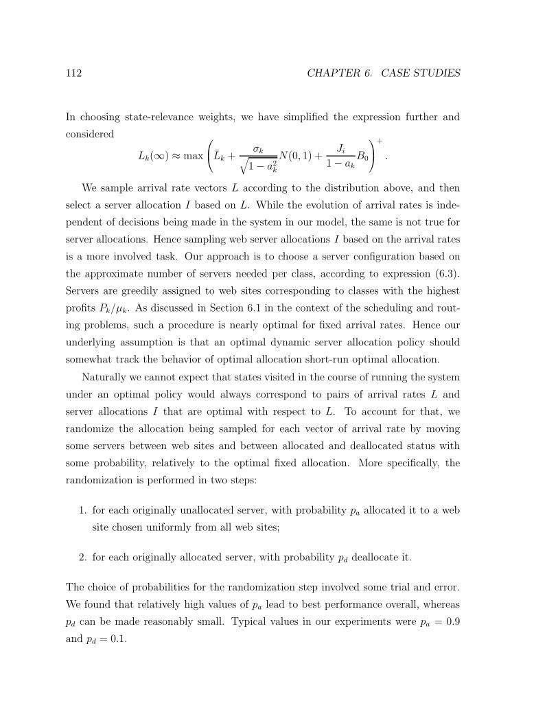
112 CHAPTER 6. CASE STUDIES
In choosing state-relevance weights, we have simplified the expression further and
considered
Lk(∞) ≈ max
Lk +
σk√1− a2
k
N(0, 1) +Ji
1− ak
B0
+
.
We sample arrival rate vectors L according to the distribution above, and then
select a server allocation I based on L. While the evolution of arrival rates is inde-
pendent of decisions being made in the system in our model, the same is not true for
server allocations. Hence sampling web server allocations I based on the arrival rates
is a more involved task. Our approach is to choose a server configuration based on
the approximate number of servers needed per class, according to expression (6.3).
Servers are greedily assigned to web sites corresponding to classes with the highest
profits Pk/µk. As discussed in Section 6.1 in the context of the scheduling and rout-
ing problems, such a procedure is nearly optimal for fixed arrival rates. Hence our
underlying assumption is that an optimal dynamic server allocation policy should
somewhat track the behavior of optimal allocation short-run optimal allocation.
Naturally we cannot expect that states visited in the course of running the system
under an optimal policy would always correspond to pairs of arrival rates L and
server allocations I that are optimal with respect to L. To account for that, we
randomize the allocation being sampled for each vector of arrival rate by moving
some servers between web sites and between allocated and deallocated status with
some probability, relatively to the optimal fixed allocation. More specifically, the
randomization is performed in two steps:
1. for each originally unallocated server, with probability pa allocated it to a web
site chosen uniformly from all web sites;
2. for each originally allocated server, with probability pd deallocate it.
The choice of probabilities for the randomization step involved some trial and error.
We found that relatively high values of pa lead to best performance overall, whereas
pd can be made reasonably small. Typical values in our experiments were pa = 0.9
and pd = 0.1.
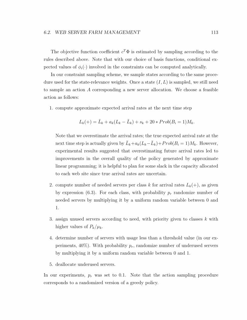
6.2. WEB SERVER FARM MANAGEMENT 113
The objective function coefficient cT Φ is estimated by sampling according to the
rules described above. Note that with our choice of basis functions, conditional ex-
pected values of φi(·) involved in the constraints can be computed analytically.
In our constraint sampling scheme, we sample states according to the same proce-
dure used for the state-relevance weights. Once a state (I, L) is sampled, we still need
to sample an action A corresponding a new server allocation. We choose a feasible
action as follows:
1. compute approximate expected arrival rates at the next time step
Lk(+) = Lk + ak(Lk − Lk) + sk + 20 ∗ Prob(Bi = 1)Mk.
Note that we overestimate the arrival rates; the true expected arrival rate at the
next time step is actually given by Lk+ak(Lk−Lk)+Prob(Bi = 1)Mk. However,
experimental results suggested that overestimating future arrival rates led to
improvements in the overall quality of the policy generated by approximate
linear programming; it is helpful to plan for some slack in the capacity allocated
to each web site since true arrival rates are uncertain.
2. compute number of needed servers per class k for arrival rates Lk(+), as given
by expression (6.3). For each class, with probability pr randomize number of
needed servers by multiplying it by a uniform random variable between 0 and
1.
3. assign unused servers according to need, with priority given to classes k with
higher values of Pk/µk.
4. determine number of servers with usage less than a threshold value (in our ex-
periments, 40%). With probability pr, randomize number of underused servers
by multiplying it by a uniform random variable between 0 and 1.
5. deallocate underused servers.
In our experiments, pr was set to 0.1. Note that the action sampling procedure
corresponds to a randomized version of a greedy policy.
114 CHAPTER 6. CASE STUDIES
6.2.6 Dealing with Action Space Complexity
The web server allocation problem suffers from complexity in the action space, in
addition to having a high-dimensional state space. In particular, a naive definition
of the problem leads to a large number of actions per state: there are two choices for
each allocated server (to keep it allocated or to deallocate it) and N + 1 choices for
each deallocated server (allocate it to each of the web sites or keep it deallocated).
An approach to dealing with the large number of actions is to split them into
sequences of actions, as described in Section 5.3.3. A natural choice is to consider
actions for each server in turn; we would have a sequence of M decisions, with each
decision being a choice from at most N +1 values. This approach does not fully solve
the problem of having a large action space; instead, we transfer the complexity to
the state space. As evidenced in the discussion of the previous section, we choose an
alternative approach: we “prune” the action space, using the structure present in the
web server allocation problem to discard actions that are most likely suboptimal in
practice.
Our pruning of the action space is based on different rules for allocating and
deallocating servers. In deciding how many servers to allocate to each web site,
we first generate a rough estimate of how many extra servers each class will need,
given by expression (6.3) and order classes according to the associated profits Pk/µk.
We then use the scoring function generated by approximate linear programming to
decide on the total number of web servers to be allocated, ranging from 0 to the total
number of free servers. Servers are allocated based upon need, following the profit-
based class ordering. In deciding how many servers to deallocate, we first estimate
their usage over the current and next time steps, and order servers based on usage.
We then consider deallocating a number of servers ranging from 0 to the number of
servers with usage under some threshold (in our experiments, 40%). We decide on
the total number of servers to be deallocated based on the scoring function generated
by approximate linear programming. Actual servers being deallocated are decided
based on the usage ordering (least used servers are deallocated first).
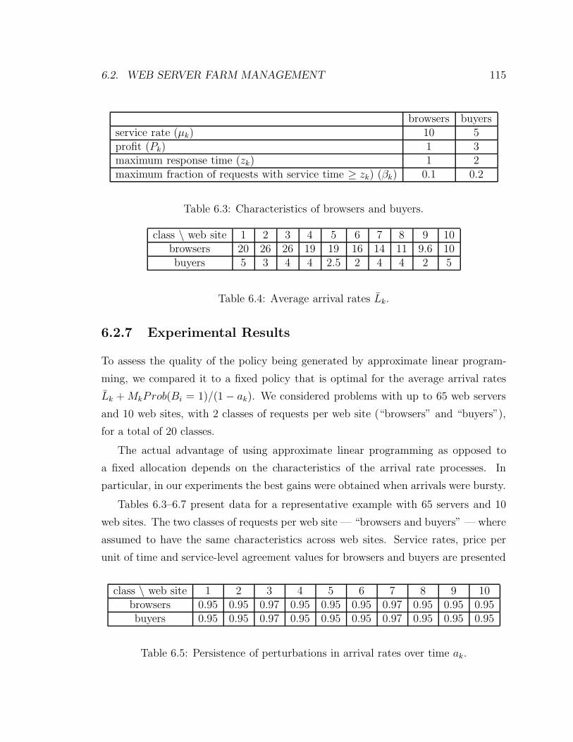
6.2. WEB SERVER FARM MANAGEMENT 115
browsers buyersservice rate (µk) 10 5profit (Pk) 1 3maximum response time (zk) 1 2maximum fraction of requests with service time ≥ zk) (βk) 0.1 0.2
Table 6.3: Characteristics of browsers and buyers.
class \ web site 1 2 3 4 5 6 7 8 9 10browsers 20 26 26 19 19 16 14 11 9.6 10buyers 5 3 4 4 2.5 2 4 4 2 5
Table 6.4: Average arrival rates Lk.
6.2.7 Experimental Results
To assess the quality of the policy being generated by approximate linear program-
ming, we compared it to a fixed policy that is optimal for the average arrival rates
Lk +MkProb(Bi = 1)/(1− ak). We considered problems with up to 65 web servers
and 10 web sites, with 2 classes of requests per web site (“browsers” and “buyers”),
for a total of 20 classes.
The actual advantage of using approximate linear programming as opposed to
a fixed allocation depends on the characteristics of the arrival rate processes. In
particular, in our experiments the best gains were obtained when arrivals were bursty.
Tables 6.3–6.7 present data for a representative example with 65 servers and 10
web sites. The two classes of requests per web site — “browsers and buyers” — where
assumed to have the same characteristics across web sites. Service rates, price per
unit of time and service-level agreement values for browsers and buyers are presented
class \ web site 1 2 3 4 5 6 7 8 9 10browsers 0.95 0.95 0.97 0.95 0.95 0.95 0.97 0.95 0.95 0.95buyers 0.95 0.95 0.97 0.95 0.95 0.95 0.97 0.95 0.95 0.95
Table 6.5: Persistence of perturbations in arrival rates over time ak.
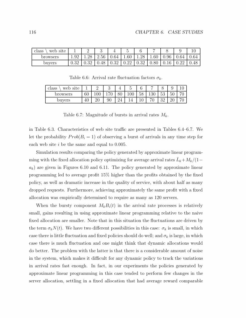
116 CHAPTER 6. CASE STUDIES
class \ web site 1 2 3 4 5 6 7 8 9 10browsers 1.92 1.28 2.56 0.64 1.60 1.28 1.60 0.96 0.64 0.64buyers 0.32 0.32 0.48 0.32 0.22 0.32 0.80 0.16 0.22 0.48
Table 6.6: Arrival rate fluctuation factors σk.
class \ web site 1 2 3 4 5 6 7 8 9 10browsers 60 100 170 80 100 58 130 53 50 70buyers 40 20 90 24 14 10 70 32 20 70
Table 6.7: Magnitude of bursts in arrival rates Mk.
in Table 6.3. Characteristics of web site traffic are presented in Tables 6.4–6.7. We
let the probability Prob(Bi = 1) of observing a burst of arrivals in any time step for
each web site i be the same and equal to 0.005.
Simulation results comparing the policy generated by approximate linear program-
ming with the fixed allocation policy optimizing for average arrival rates Lk+Mk/(1−ak) are given in Figures 6.10 and 6.11. The policy generated by approximate linear
programming led to average profit 15% higher than the profits obtained by the fixed
policy, as well as dramatic increase in the quality of service, with about half as many
dropped requests. Furthermore, achieving approximately the same profit with a fixed
allocation was empirically determined to require as many as 120 servers.
When the bursty component MkBi(t) in the arrival rate processes is relatively
small, gains resulting in using approximate linear programming relative to the naive
fixed allocation are smaller. Note that in this situation the fluctuations are driven by
the term σkN(t). We have two different possibilities in this case: σk is small, in which
case there is little fluctuation and fixed policies should do well; and σk is large, in which
case there is much fluctuation and one might think that dynamic allocations would
do better. The problem with the latter is that there is a considerable amount of noise
in the system, which makes it difficult for any dynamic policy to track the variations
in arrival rates fast enough. In fact, in our experiments the policies generated by
approximate linear programming in this case tended to perform few changes in the
server allocation, settling in a fixed allocation that had average reward comparable
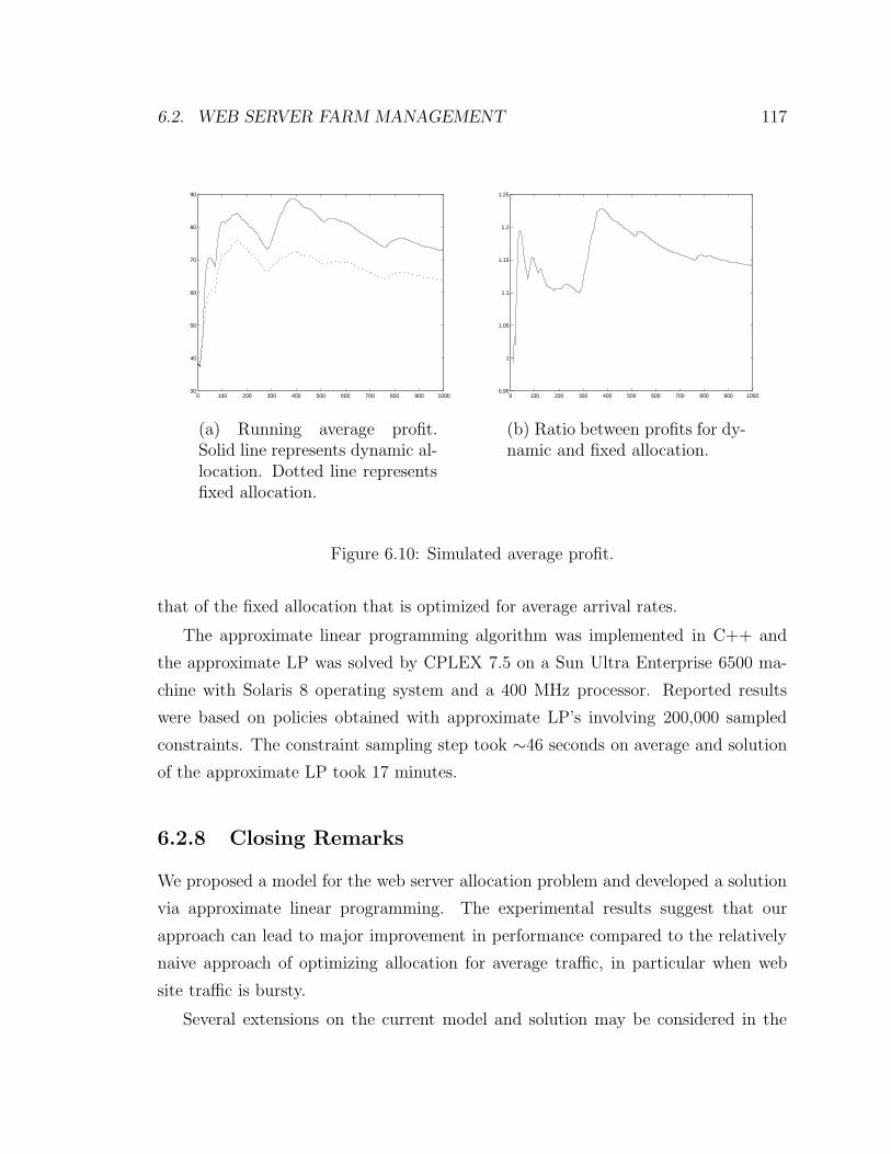
6.2. WEB SERVER FARM MANAGEMENT 117
0 100 200 300 400 500 600 700 800 900 100030
40
50
60
70
80
90
(a) Running average profit.Solid line represents dynamic al-location. Dotted line representsfixed allocation.
0 100 200 300 400 500 600 700 800 900 10000.95
1
1.05
1.1
1.15
1.2
1.25
(b) Ratio between profits for dy-namic and fixed allocation.
Figure 6.10: Simulated average profit.
that of the fixed allocation that is optimized for average arrival rates.
The approximate linear programming algorithm was implemented in C++ and
the approximate LP was solved by CPLEX 7.5 on a Sun Ultra Enterprise 6500 ma-
chine with Solaris 8 operating system and a 400 MHz processor. Reported results
were based on policies obtained with approximate LP’s involving 200,000 sampled
constraints. The constraint sampling step took ∼46 seconds on average and solution
of the approximate LP took 17 minutes.
6.2.8 Closing Remarks
We proposed a model for the web server allocation problem and developed a solution
via approximate linear programming. The experimental results suggest that our
approach can lead to major improvement in performance compared to the relatively
naive approach of optimizing allocation for average traffic, in particular when web
site traffic is bursty.
Several extensions on the current model and solution may be considered in the
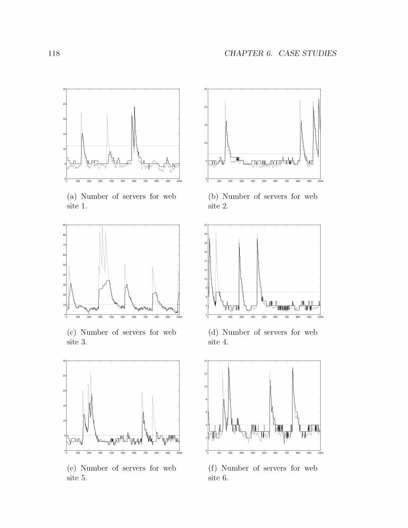
118 CHAPTER 6. CASE STUDIES
0 100 200 300 400 500 600 700 800 900 10000
5
10
15
20
25
30
(a) Number of servers for website 1.
0 100 200 300 400 500 600 700 800 900 10000
5
10
15
20
25
(b) Number of servers for website 2.
0 100 200 300 400 500 600 700 800 900 10000
10
20
30
40
50
60
70
80
90
(c) Number of servers for website 3.
0 100 200 300 400 500 600 700 800 900 10002
4
6
8
10
12
14
16
18
20
22
(d) Number of servers for website 4.
0 100 200 300 400 500 600 700 800 900 10000
5
10
15
20
25
30
(e) Number of servers for website 5.
0 100 200 300 400 500 600 700 800 900 10000
2
4
6
8
10
12
14
(f) Number of servers for website 6.
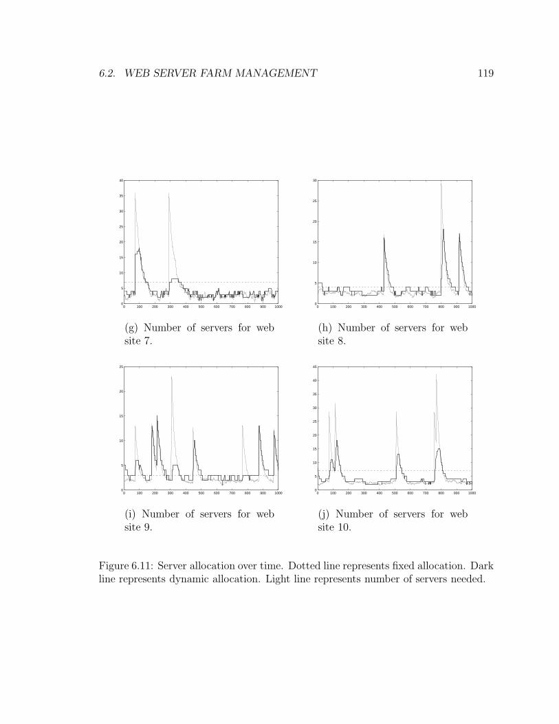
6.2. WEB SERVER FARM MANAGEMENT 119
0 100 200 300 400 500 600 700 800 900 10000
5
10
15
20
25
30
35
40
(g) Number of servers for website 7.
0 100 200 300 400 500 600 700 800 900 10000
5
10
15
20
25
30
(h) Number of servers for website 8.
0 100 200 300 400 500 600 700 800 900 10000
5
10
15
20
25
(i) Number of servers for website 9.
0 100 200 300 400 500 600 700 800 900 10000
5
10
15
20
25
30
35
40
45
(j) Number of servers for website 10.
Figure 6.11: Server allocation over time. Dotted line represents fixed allocation. Darkline represents dynamic allocation. Light line represents number of servers needed.

120 CHAPTER 6. CASE STUDIES
future:
• More extensive comparison with other heuristics;
• Refinement of the arrival rate processes, with the possibility of including fore-
casts and accounting for cyclical patterns often observed in Internet traffic;
• Refinement of the choice of basis functions;
• Further development of the action space pruning strategies;
• Integration with the problems of scheduling and routing, by considering all of
them in the dynamic programming framework, rather than solving the first two
by a fluid model approximation;
• Consideration of capacity planning, where the number of servers does not remain
fixed but may increase as new servers are acquired over time.
Chapter 7
Conclusions
Over the years, interest in approximate dynamic programming has been fueled by
stories of empirical success in applications in areas that span from games [48] to dy-
namic resource allocation [12, 36, 45, 59] to finance [32, 40]. Nevertheless, practical
use of the methodology remains limited by a lack of systematic guidelines for imple-
mentation and theoretical guarantees, which reflects on the amount of trial and error
involved in each of the success stories found in the literature and on the difficulty in
duplicating the same success in other applications. I believe that until a thorough
understanding of approximate dynamic programming is achieved and algorithms be-
come fairly streamlined, the methodology will not fulfill its potential for becoming a
widely used tool assisting decision-making in complex-systems.
Part of the research presented in this dissertation represents an effort toward de-
veloping more streamlined approximate dynamic programming algorithms and bridg-
ing the gap between empirical success and theoretical guarantees. In particular, the
analysis in Chapters 3 and 4 sheds light on the impact of the algorithm parameters
involved in approximate linear programming on the overall performance of the algo-
rithm. Performance of the approximate linear programming algorithm is well defined
by bounds on the error in the approximation of the optimal value function and on
the performance of the policy ultimately generated. The same bounds provide some
guidance on the choice of basis functions. We also achieve relatively good understand-
ing of the role of state-relevance weights, which may help reduce the amount of trial
121
122 CHAPTER 7. CONCLUSIONS
and error involved in successfully implementing approximate linear programming, as
compared to other approximate dynamic programming algorithms.
The results in Chapter 5 represent a step toward making approximate linear pro-
gramming applicable to a wider number of applications; implementations of the al-
gorithm described in the literature typically require problems with special structure
making exact solution of the approximate LP tractable despite the huge number of
constraints [24, 39, 42], or involve a number of heuristic argument lacking theoretical
guarantees [49, 50]. Our constraint sampling algorithm is the first method designed
for general MDP’s.
It should be noted that, while the results presented here represent advances in the
understanding and development of approximate dynamic programming, questions still
outnumber answers in this area. I believe that an ideal method should be able to
• distinguish between scenarios and options that are relevant and others that can
be neglected;
• allow for the incorporation of prior knowledge about the problem obtained in
the derivation and experimentation with heuristic solutions or through common
sense;
• offer theoretical guarantees of performance so that successes and failures are
easily explained;
• be reliable and simple enough to be used with confidence by practitioners in
industry.
Approximate linear programming satisfies some of these conditions, but as illustrated
in the case studies of Chapter 6, there is still some amount of trial and error involved
in implementation of the algorithm. It is unlikely that we will ever have a fully au-
tomated algorithm for decision-making in complex systems. However, the conditions
above serve as a guideline for desirable properties we should seek in the development
of approximate dynamic programming algorithms.
There is much space for further developments in approximate linear programming.
We mention a few possibilities:
123
• In principle, approximate linear programming requires explicit knowledge of the
costs and transition probabilities in the system. Implementation is still possible
if a system simulator is available, provided that simulation of transitions starting
in any given state can be performed multiple times. In this case, one can build
estimates of the costs and conditional expected values of the basis functions
involved in the approximate LP constraints for each of the sampled states. It
would be desirable to determine the impact of inaccuracies in these estimates
on the overall performance of the approximate LP.
• Some approximate dynamic programming algorithms can run online, i.e., adap-
tively learn policies as the system runs in real time. This is particularly desirable
if the system parameters are slowly changing over time because the method can
then adapt to those changes. Using approximate linear programming in such
instances requires re-running the algorithm from time to time when the system
parameters have changed “enough.” It would be useful to have a characteriza-
tion of how much change is “enough,” determining when it would be useful to
re-run the algorithm.
• Some of the results presented here suggest iterative implementation of the
method, with parameters changing over time; for instance, the bounds on the
performance of the ALP policy suggest adaptive generation of state-relevance
weights. Turning approximate linear programming into an iterative method
raises new questions, such as whether the algorithm converges and, if it does,
what kinds of performance guarantees can be offered.
• As indicated in Chapter 5, there are many open questions concerning the con-
straint sampling algorithm: What is the impact of not using the ideal distri-
bution prescribed by the method for sampling the constraints? How can one
efficiently identify a set of constraints ensuring boundedness of the solution of
the reduced approximate LP? Can we improve the bounds on the number of
constraints needed for near-feasibility?
Perhaps the most important question that has not been addressed here refers to

124 CHAPTER 7. CONCLUSIONS
the choice of basis functions or, more generally, of an approximation architecture.
Some fairly general approaches to choosing basis functions are described in the case
studies in Chapter 6, such as mapping states to smooth features and then using
basis functions that are polynomial functions of features. However, such approaches
lack in rigor. It is likely that there will always be some amount of problem-specific
analysis and experimentation involved in the design of an approximation architecture.
Nevertheless, it would be interesting to explore whether there exist canonical choices
of architectures at least in some application domains, or what kinds of algorithms one
could design for successively refining the choice of approximation architecture.

Bibliography
[1] L. Baird. Gradient descent for general reinforcement learning. In Advances in
Neural Information Processing Systems, volume 11, 1998.
[2] J. Baxter and P. Bartlett. Direct gradient-based reinforcement learning. Techni-
cal report, Research School of Information Sciences and Engineering, Australian
National University, 1999.
[3] R.E. Bellman and S.E. Dreyfus. Functional approximations and dynamic pro-
gramming. Mathematical Tables and Other Aids to Computation, 13:247–251,
1959.
[4] D. Bertsekas. Dynamic Programming and Optimal Control. Athena Scientific,
1995.
[5] D. Bertsekas and J.N. Tsitsiklis. Neuro-Dynamic Programming. Athena Scien-
tific, 1996.
[6] D. Bertsimas, D. Gamarnik, and J.N. Tsitsiklis. Performance of multiclass
Markovian queueing networks via piecewise linear Lyapunov functions. Sub-
mitted to Annals of Applied Probability, 2000.
[7] C.M. Bishop. Neural Networks for Pattern Recognition. Oxford University Press,
1995.
[8] D. Blackwell. Discrete dynamic programming. Annals of Mathematical Statistics,
33(2):719–726, 1962.
125
126 BIBLIOGRAPHY
[9] V. Borkar. A convex analytic approach to Markov decision processes. Probability
Theory and Related Fields, 78:583–602, 1988.
[10] R-R. Chen and S. Meyn. Value iteration and optimization of multiclass queueing
networks. Queueing Systems, 32:65–97, 1999.
[11] V.C.P. Chen, D. Ruppert, and C.A. Shoemaker. Applying experimental design
and regression splines to high-dimensional continuous-state stochast dynamic
programming. Operations Research, 47(1):38–53, 1999.
[12] R.H. Crites and A.G. Barto. Improving elevator performance using reinforcement
learning. In Advances in Neural Information Processing Systems, volume 8, 1996.
[13] P. Dayan. The convergence of TD(λ) for general λ. Machine Learning, 8:341–362,
1992.
[14] D.P. de Farias and B. Van Roy. On the existence of fixed points for appproximate
value iteration and temporal-difference learning. Journal of Optimization Theory
and Applications, 105(3), 2000.
[15] D.P. de Farias and B. Van Roy. The linear programming approach to approximate
dynamic programming. Conditionally accepted to Operations Research, 2001.
[16] D.P. de Farias and B. Van Roy. On constraint sampling in the linear program-
ming approach to approximate dynamic programming. Conditionally accepted
to Mathematics of Operations Research, 2001.
[17] G. de Ghellinck. Les problemes de decisions sequentielles. Cahiers du Centre
d’Etudes de Recherche Operationnelle, 2:161–179, 1960.
[18] E.V. Denardo. On linear programming in a Markov decision problem. Manage-
ment Science, 16(5):282–288, 1970.
[19] F. D’Epenoux. A probabilistic production and inventory problem. Management
Science, 10(1):98–108, 1963.
BIBLIOGRAPHY 127
[20] R.M. Dudley. Uniform Central Limit Theorems. Cambridge University Press,
Cambridge, 1998.
[21] R. Durrett. Probability: Theory and Examples. Duxbury Press, 1995.
[22] G. Gordon. Approximate Solutions to Markov Decision Processess. PhD thesis,
Carneggie Mellon University, 1999.
[23] M. Grotschel and O. Holland. Solution of large-scale symmetric travelling sales-
man problems. Mathematical Programming, 51:141–202, 1991.
[24] C. Guestrin, D. Koller, and R. Parr. Efficient solution algorithms for factored
MDPs. Submitted to Journal of Artificial Intelligence Research, 2001.
[25] S. Haykin. Neural Networks: A Comprehensive Formulation. McMillan, 1994.
[26] A. Hordijk and L.C.M. Kallenberg. Linear programming and Markov decision
chains. Management Science, 25:352–362, 1979.
[27] V.R. Konda and V.S. Borkar. Actor-critic type learning algorithms for Markov
decision processes. SIAM Journal on Control and Optimization, 38(1):94–133,
1999.
[28] V.R. Konda and J.N. Tsitsiklis. Actor-critic algorithms. Submitted to the SIAM
Journal on Control and Optimization, 2001.
[29] P.R. Kumar and S. Meyn. Duality and linear programs for stability and perfor-
mance analysis of queueing networks and scheduling policies. IEEE Transactions
on Automatic Control, 41(1):4–17, 1996.
[30] P.R. Kumar and T.I. Seidman. Dynamic instabilities and stabilization methods
in distributed real-time scheduling of manufacturing systems. IEEE Transactions
on Automatic Control, 35(3):289–298, 1990.
[31] Z. Liu, M.S. Squillante, and J.L. Wolf. On maximizing service-level-agreement
profits. Working paper, IBM T.J. Watson Research Center, 2000.
128 BIBLIOGRAPHY
[32] F. Longstaff and E.S. Schwartz. Valuing American options by simulation: A
simple least squares approach. The Review of Financial Studies, 14:113–147,
2001.
[33] D.G. Luenberger. Optimization by Vector Space Methods. Wiley-Interscience,
1969.
[34] A.S. Manne. Linear programming and sequential decisions. Management Science,
6(3):259–267, 1960.
[35] P. Marbach. Simulation-Based Methods for Markov Decision Processes. PhD
thesis, Massachussetts Institute of Technology, 1998.
[36] P. Marbach, O. Mihatsch, and J.N. Tsitsiklis. Call admission control and routing
in integrated service networks using neuro-dynamic programming. IEEE Journal
on Selected Areas in Communications, 18(2):197–208, 2000.
[37] P. Marbach and J.N. Tsitsiklis. Simulation-based optimization of Markov reward
processes. IEEE Transactions on Automatic Control, 46(2):191–209, 2001.
[38] S.P. Meyn. Sequencing and routing in multiclass queueing networks, part i:
Feedback regulation. To appear, SIAM Journal of Control and Optimization,
2001.
[39] J.R. Morrison and P.R. Kumar. New linear program performance bounds
for queueing networks. Journal of Optimization Theory and Applications,
100(3):575–597, 1999.
[40] B. Van Roy and J.N. Tsitsiklis. Regression methods for pricing complex
American-style options. IEEE Transactions on Neural Networks, 12(4):694–703,
2001.
[41] A.N. Rybko and A.L. Stolyar. On the ergodicity of stochastic processes describing
the operation of open queueing networks. Problemy Peredachi Informatsii, 28:3–
26, 1992.

BIBLIOGRAPHY 129
[42] D. Schuurmans and R. Patrascu. Direct value-approximation for factored MDPs.
In Advances in Neural Information Processing Systems, volume 14, 2001.
[43] P. Schweitzer and A. Seidmann. Generalized polynomial approximations in
Markovian decision processes. Journal of Mathematical Analysis and Applica-
tions, 110:568–582, 1985.
[44] C. Shannon. Programming a digital computer for playing chess. Philosophical
Magazine, 41:356–375, 1950.
[45] S. Singh and D. Bertsekas. Reinforcement learning for dynamic channel allocation
in cellular telephone systems. In Advances in Neural Information Processing
Systems, volume 9, 1997.
[46] R. Sutton, D. McAllester, S. Singh, and Y. Mansour. Policy gradient methods
for reinforcement learning with function approximation. In Advances in Neural
Information Processing Systems, volume 12, pages 1057–1063, 2000.
[47] R.S. Sutton. Learning to predict by the methods of temporal differences. Machine
Learning, 3:9–44, 1988.
[48] G.J. Tesauro. Temporal difference learning and TD-gammon. Communications
of the ACM, 38:58–68, 1995.
[49] M. Trick and S. Zin. A linear programming approach to solving dynamic pro-
grams. Unpublished manuscript, 1993.
[50] M. Trick and S. Zin. Spline approximations to value functions: A linear pro-
gramming approach. Macroeconomic Dynamics, 1, 1997.
[51] J.N. Tsitsiklis and B. Van Roy. An analysis of temporal-difference learning with
function approximation. IEEE Transactions on Automatic Control, 42(5):674–
690, 1997.
[52] B. Van Roy. Feature-based methods for large scale dynamic programming. Ma-
chine Learning, 22:59–94, 1996.
130 BIBLIOGRAPHY
[53] B. Van Roy. Learning and Value Function Approximation in Complex Decision
Processes. PhD thesis, Massachusetts Institute of Technology, 1998.
[54] B. Van Roy. Neuro-dynamic programming: Overview and recent trends. In
E. Feinberg and A. Schwartz, editors, Markov Decision Processes: Models, Meth-
ods, Directions, and Open Problems. Kluwer, 2000.
[55] A.F. Veinott Jr. Discrete dynamic programming with sensitive discount opti-
mality criteria. Annals of Mathematical Statistics, 40(5):1635–1660, 1969.
[56] A.F. Veinott Jr. Lectures in dynamic programming and stochastic control, Spring
1999. Lecture notes for EESOR 351, Department of Engineering-Economic Sys-
tems and Operations Research, Stanford University.
[57] M. Vidyasagar. A Theory of Learning and Generalization. Springer, London,
1997.
[58] R.J. Williams. Simple statistical gradient-following algorithms for connectionist
reinforcement learning. Machine Learning, 8:229–256, 1992.
[59] W. Zhang and T.G. Dietterich. High-performance job-shop scheduling with a
time-delay TD(λ) network. In Advances in Neural Information Processing Sys-
tems, volume 8, 1996.