Embed Size (px)
Citation preview
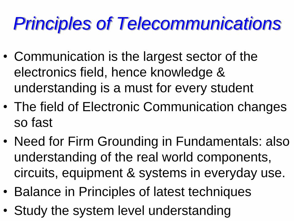
Principles of Telecommunications
• Communication is the largest sector of the
electronics field, hence knowledge &
understanding is a must for every student
• The field of Electronic Communication changes
so fast
• Need for Firm Grounding in Fundamentals: also
understanding of the real world components,
circuits, equipment & systems in everyday use.
• Balance in Principles of latest techniques
• Study the system level understanding
EEB317 Principles of Telecoms
•Signals & Systems
•Amplitude Modulation
•Angle Modulation
•Detection & Demodulation
•Noise in Communications System
Signals & Systems
•Classification
•Power & Energy Spectral Density
•Correlation
•Fourier Series & Transform
•Convolution
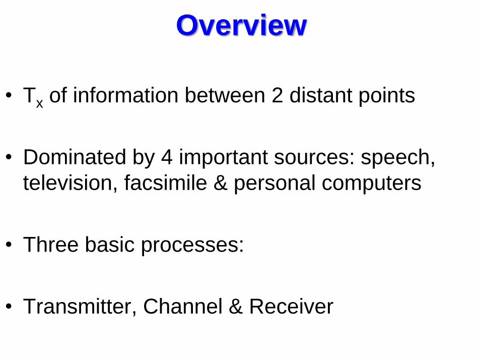
Overview
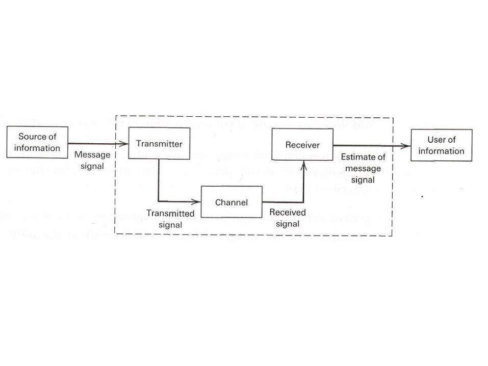
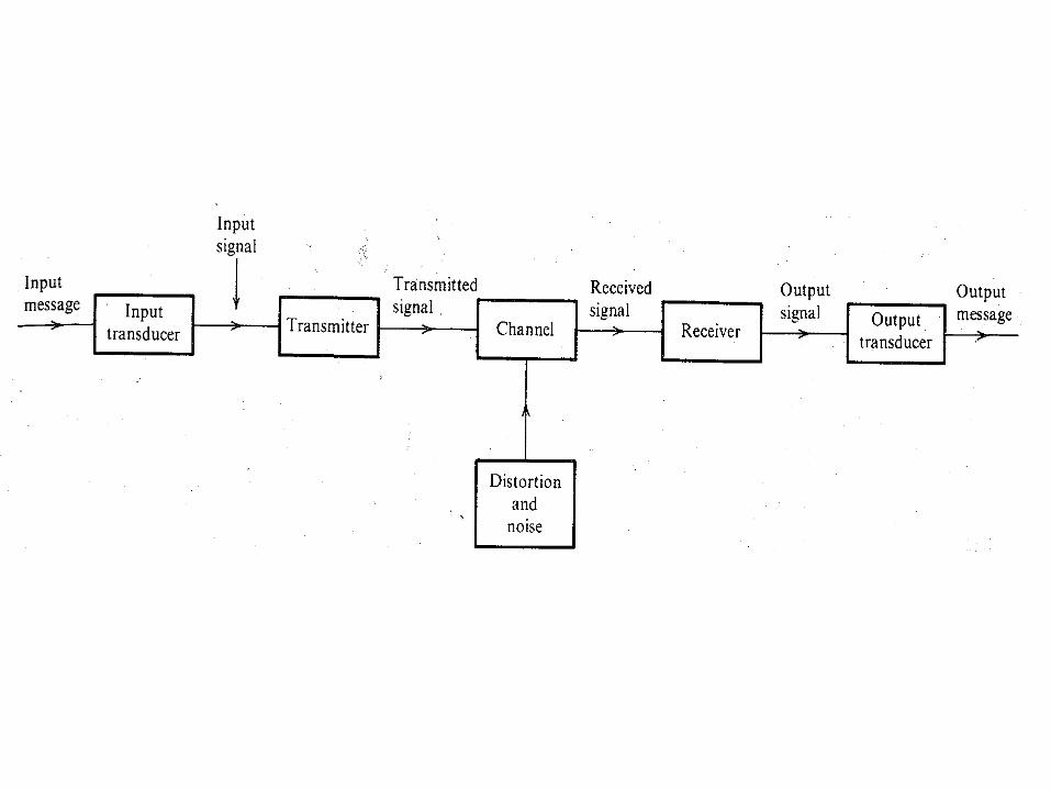
• Tx of information between 2 distant points
• Dominated by 4 important sources: speech,
television, facsimile & personal computers
• Three basic processes:
• Transmitter, Channel & Receiver
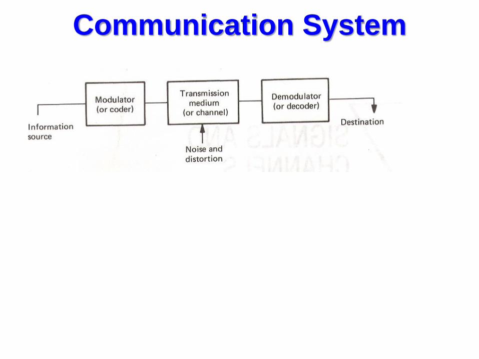
Communication System
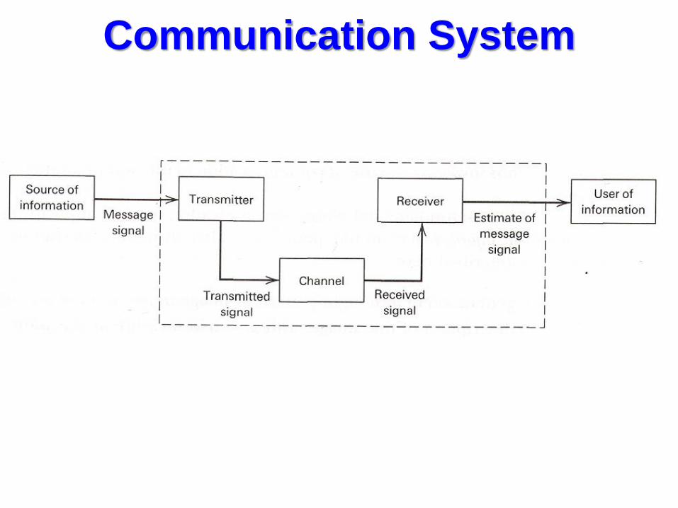
Communication System
Classification of signals & Systems• A system is an interacting set of physical
objects or physical conditions called system
components
• A signal: set of information or data. Can be
input, output or internal
• Signals may be functions of independent
variables such as time, distance, force, position,
pressure, temp … for simplicity only time will be
used in this class
• Mathematical models are mathematical
equations that represent signals & systems
• They permit quantitative analysis and design of
signals & systems
• Continuous-time signal x(t), has a value
specified for all points in time, & a continuous-
time system operates on and produces
continuous-time signals
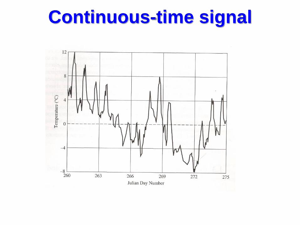
Continuous-time signal
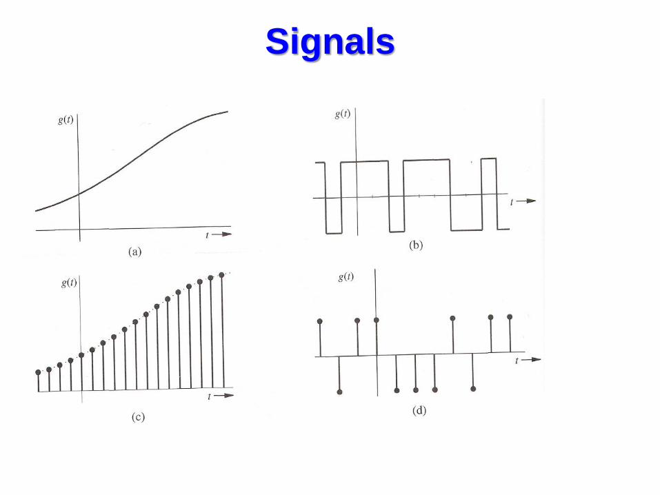
Signals
Signals• Discrete-time signal: Signal specified only at
discrete values
• Analog signal: Signal whose amplitude can
take on any value in a continuous range
• Digital signal: Signal whose amplitude can
take on only finite number of values (M-ary)
• Periodic signal: Signal g(t) is periodic if for
some +ve constant T0 (period):
)()( 0Ttgtg
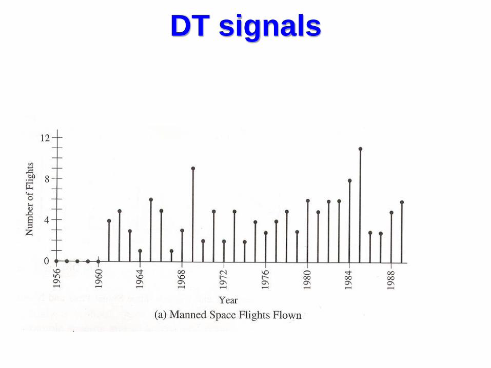
DT signals
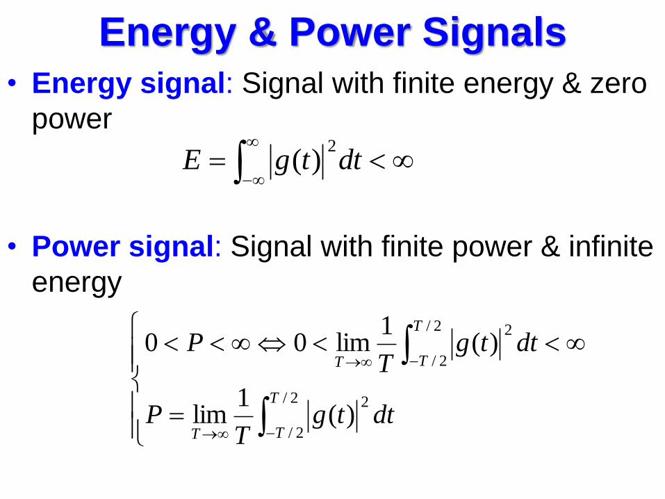
Energy & Power Signals• Energy signal: Signal with finite energy & zero
power
• Power signal: Signal with finite power & infinite
energy
dttgE
2)(
2/
2/
2
2/
2/
2
)(1
lim
)(1
lim00
T
TT
T
TT
dttgT
P
dttgT
P
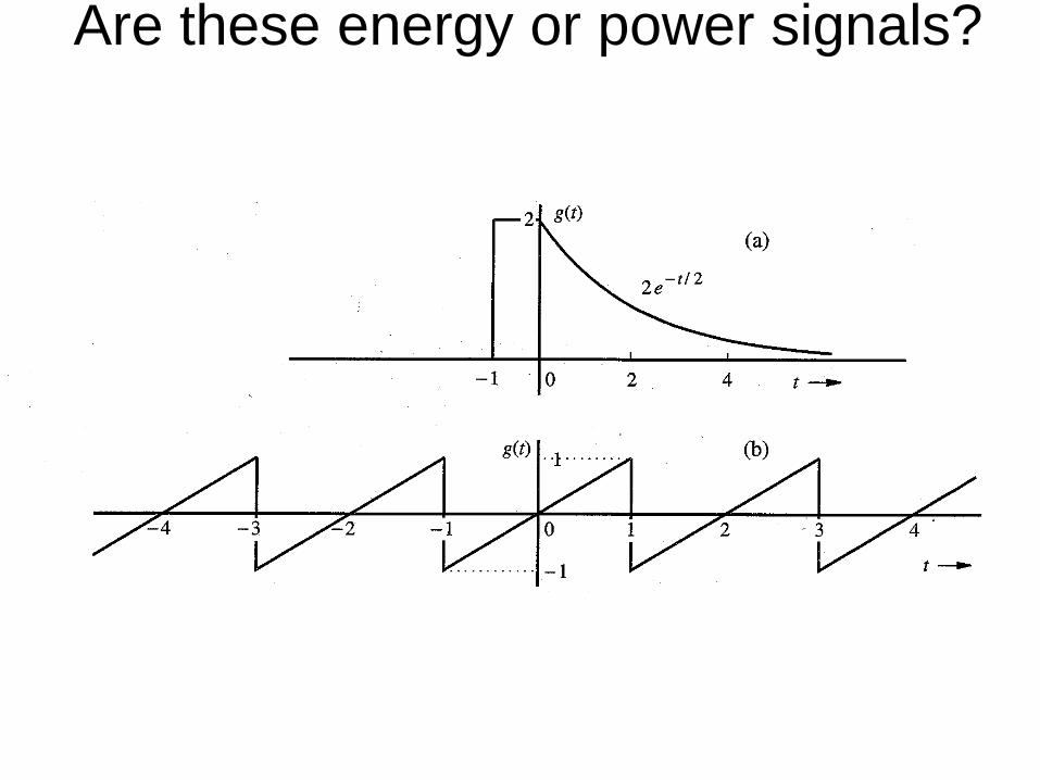
Are these energy or power signals?
•
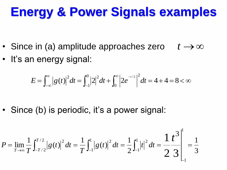
Energy & Power Signals examples
• Since in (a) amplitude approaches zero
• It’s an energy signal:
• Since (b) is periodic, it’s a power signal:
t
84422)(0
20
1
22 2/
dtedtdttgEt
3
13
2
1)(
1)(
1lim
32
11
1
1
1
21
1
22/
2/
2
t
dttdttgT
dttgT
PT
TT
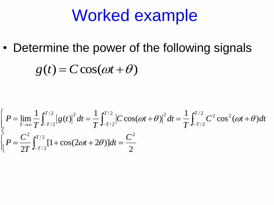
Worked example
• Determine the power of the following signals
)cos()( tCtg
2/
2/
22
2/
2/
222/
2/
22/
2/
2
2)]22cos(1[
2
)(cos1
)cos(1
)(1
lim
T
T
T
T
T
T
T
TT
Cdtt
T
CP
dttCT
dttCT
dttgT
P
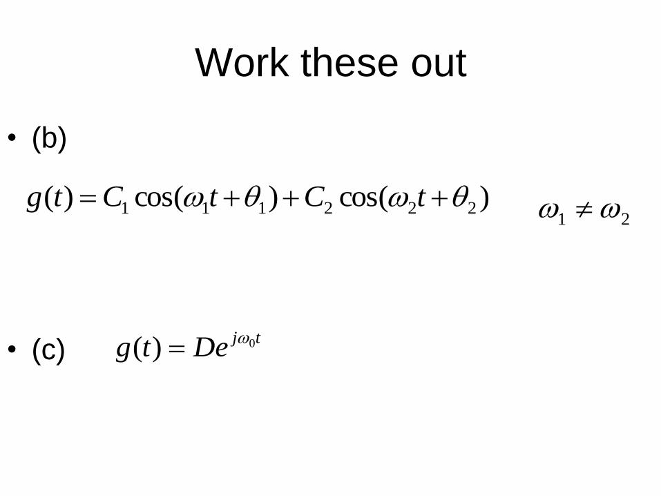
Work these out
• (b)
• (c)
)cos()cos()( 222111 tCtCtg21
tjDetg 0)(
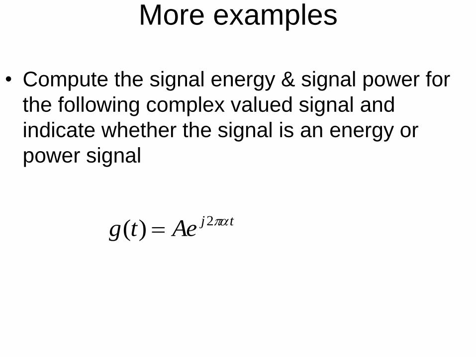
More examples
• Compute the signal energy & signal power for
the following complex valued signal and
indicate whether the signal is an energy or
power signal
tjAetg 2)(
More examples
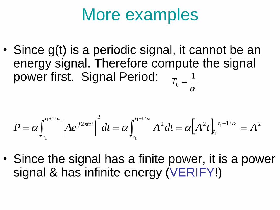
• Since g(t) is a periodic signal, it cannot be an energy signal. Therefore compute the signal power first. Signal Period:
• Since the signal has a finite power, it is a power signal & has infinite energy (VERIFY!)
10 T
2/1222
2 1
1
/11
1
/11
1
AtAdtAdtAePt
t
tjt
t
t
t
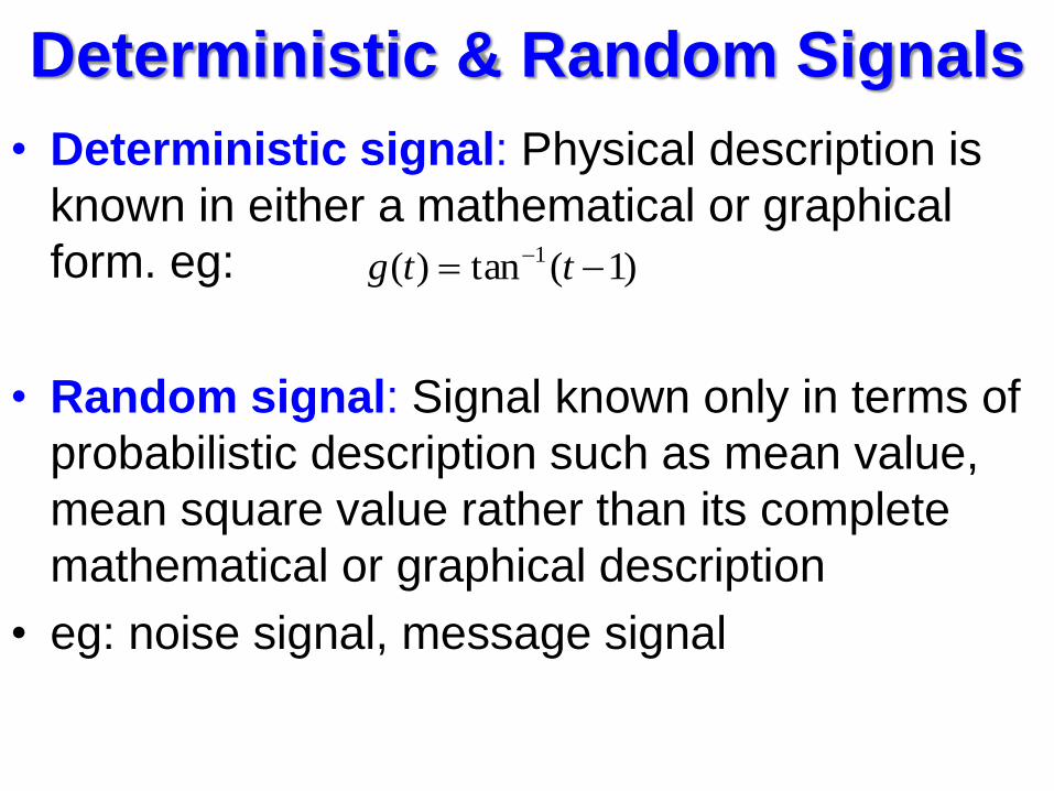
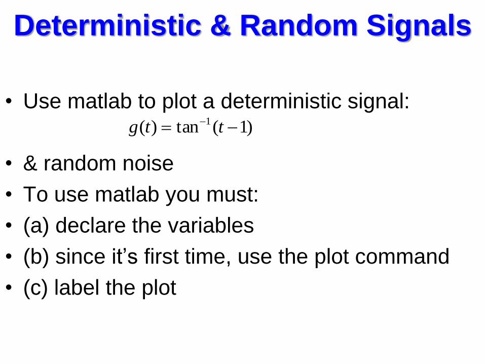
Deterministic & Random Signals
• Deterministic signal: Physical description is
known in either a mathematical or graphical
form. eg:
• Random signal: Signal known only in terms of
probabilistic description such as mean value,
mean square value rather than its complete
mathematical or graphical description
• eg: noise signal, message signal
)1(tan)( 1 ttg
Deterministic & Random Signals
• Use matlab to plot a deterministic signal:
• & random noise
• To use matlab you must:
• (a) declare the variables
• (b) since it’s first time, use the plot command
• (c) label the plot
)1(tan)( 1 ttg
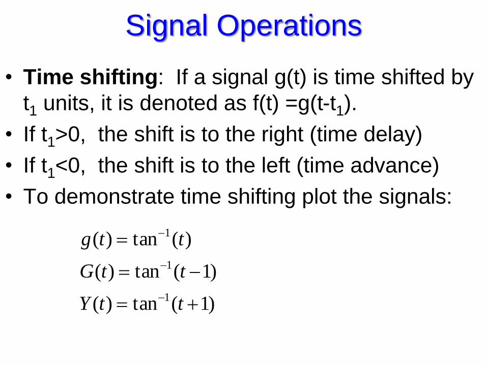
Signal Operations
• Time shifting: If a signal g(t) is time shifted by
t1 units, it is denoted as f(t) =g(t-t1).
• If t1>0, the shift is to the right (time delay)
• If t1<0, the shift is to the left (time advance)
• To demonstrate time shifting plot the signals:
)1(tan)(
)1(tan)(
)(tan)(
1
1
1
ttY
ttG
ttg
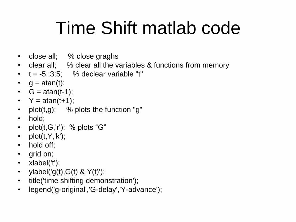
Time Shift matlab code
• close all; % close graghs
• clear all; % clear all the variables & functions from memory
• t = -5:.3:5; % declear variable "t"
• g = atan(t);
• G = atan(t-1);
• Y = atan(t+1);
• plot(t,g); % plots the function "g"
• hold;
• plot(t,G,'r'); % plots “G”
• plot(t,Y,'k');
• hold off;
• grid on;
• xlabel('t');
• ylabel('g(t),G(t) & Y(t)');
• title('time shifting demonstration');
• legend('g-original','G-delay','Y-advance');
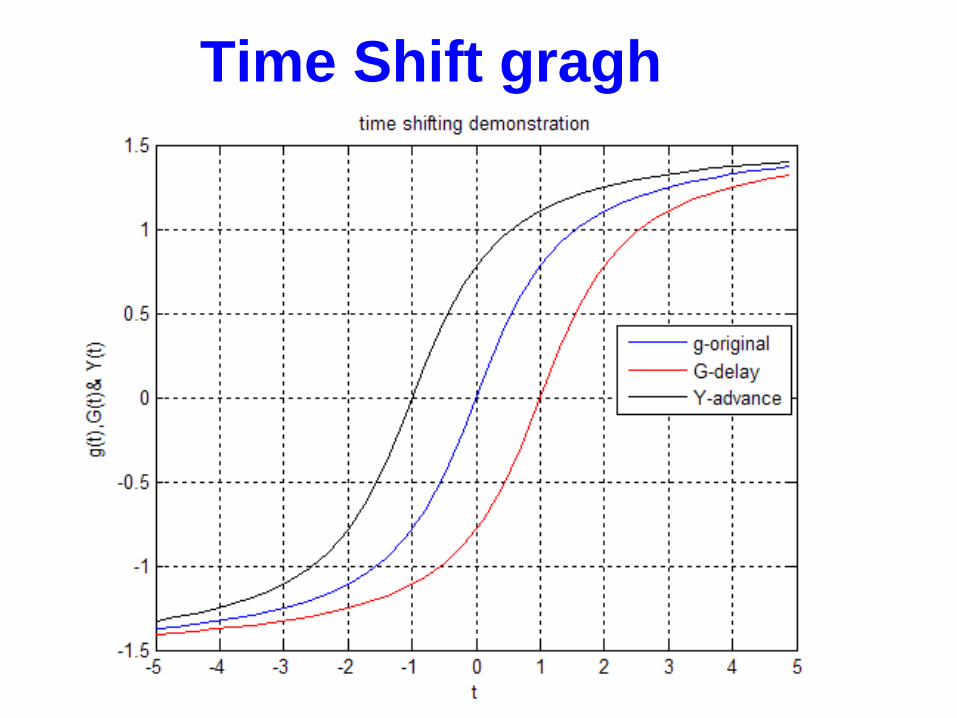
Time Shift gragh
Signal Operations
• Time Scaling: Compression or expansion of a signal
• Signal f(t) is g(t) compressed by a factor of ‘a’ if f(t) = g(at), therefore f(t/a) = g(t) for a>1
• Similarly f(t) is g(t) expanded (slowed down) by a factor of ‘a’ if f(t) = g(t/a), therefore f(at) = g(t) for a<1
• To time-scale a signal by a factor of ‘a’, replace t with at.
• If a > 1 the scaling is compressed & if a < 1, the scaling is expanded.
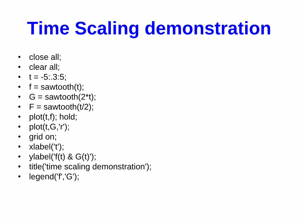
Time Scaling demonstration
• close all;
• clear all;
• t = -5:.3:5;
• f = sawtooth(t);
• G = sawtooth(2*t);
• F = sawtooth(t/2);
• plot(t,f); hold;
• plot(t,G,'r');
• grid on;
• xlabel('t');
• ylabel('f(t) & G(t)');
• title('time scaling demonstration');
• legend('f','G');
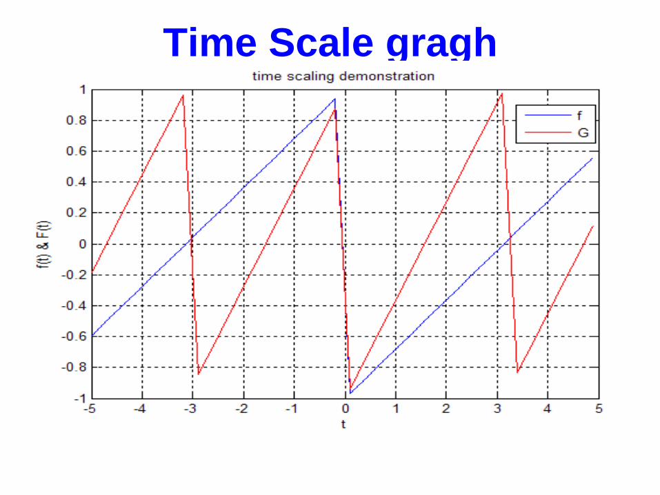
Time Scale gragh
Signal Operations
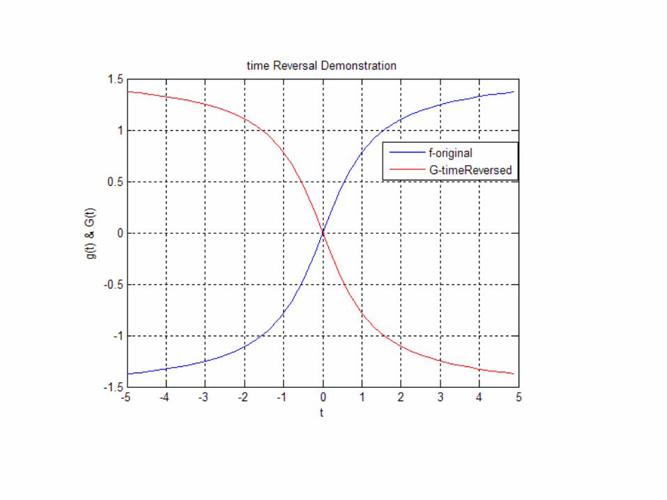
• Time Reversal/Inversion/Folding:
• To time reverse a signal, replace t with –t
• If f(t) is a time resersal of g(t) then
• f(t)=g(-t)
• See the matlab code of g(-t)
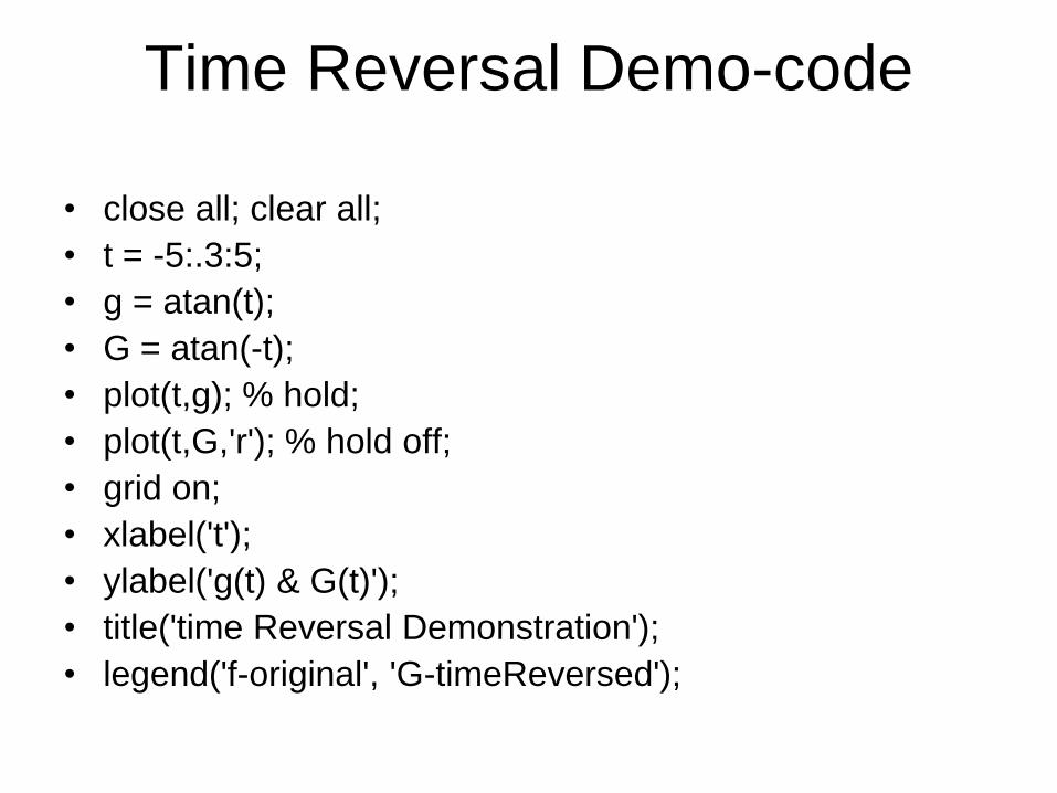
Time Reversal Demo-code
• close all; clear all;
• t = -5:.3:5;
• g = atan(t);
• G = atan(-t);
• plot(t,g); % hold;
• plot(t,G,'r'); % hold off;
• grid on;
• xlabel('t');
• ylabel('g(t) & G(t)');
• title('time Reversal Demonstration');
• legend('f-original', 'G-timeReversed');
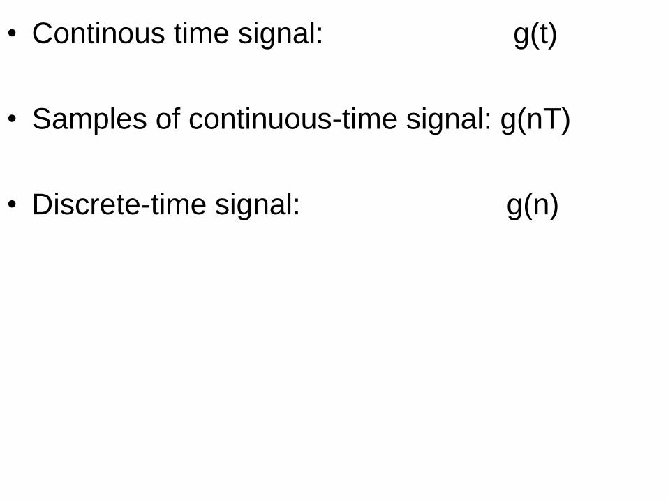
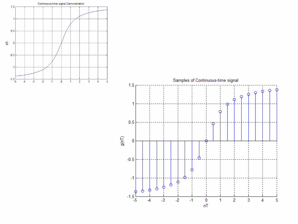
• Continous time signal: g(t)
• Samples of continuous-time signal: g(nT)
• Discrete-time signal: g(n)
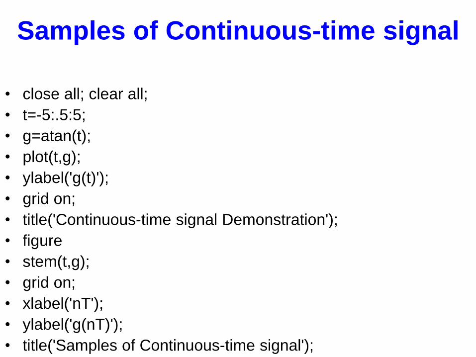
Samples of Continuous-time signal
• close all; clear all;
• t=-5:.5:5;
• g=atan(t);
• plot(t,g);
• ylabel('g(t)');
• grid on;
• title('Continuous-time signal Demonstration');
• figure
• stem(t,g);
• grid on;
• xlabel('nT');
• ylabel('g(nT)');
• title('Samples of Continuous-time signal');
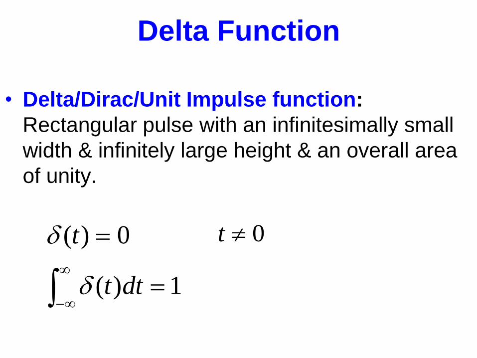
Delta Function
• Delta/Dirac/Unit Impulse function:
Rectangular pulse with an infinitesimally small
width & infinitely large height & an overall area
of unity.
1)(
0)(
dtt
t
0t
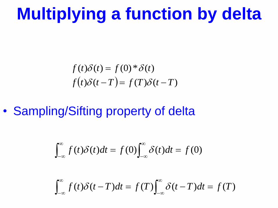
Multiplying a function by delta
• Sampling/Sifting property of delta
)()(()
)(*)0()()(
TtTfTttf
tfttf
)()()()()(
)0()()0()()(
TfdtTtTfdtTttf
fdttfdtttf
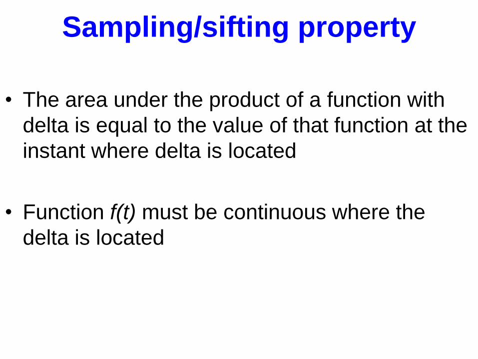
Sampling/sifting property
• The area under the product of a function with
delta is equal to the value of that function at the
instant where delta is located
• Function f(t) must be continuous where the
delta is located
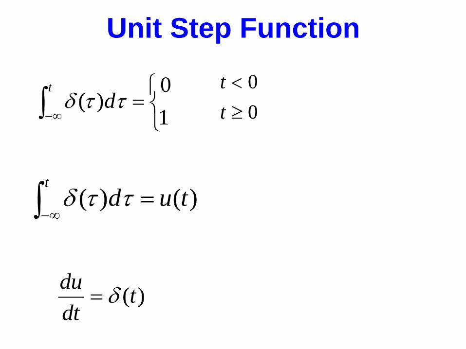
Unit Step Function
t
d1
0)(
0
0
t
t
t
tud )()(
)(tdt
du
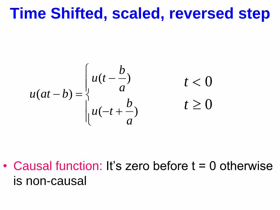
Time Shifted, scaled, reversed step
• Causal function: It’s zero before t = 0 otherwise
is non-causal
)(
)(
)(
a
btu
a
btu
batu0
0
t
t
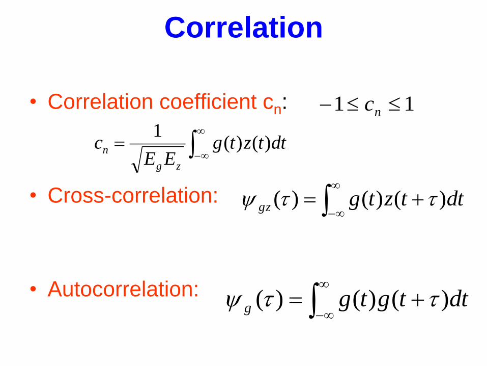
Correlation
• Correlation coefficient cn:
• Cross-correlation:
• Autocorrelation:
11 nc
dttztg
EEc
zg
n )()(1
dttztggz )()()(
dttgtgg )()()(
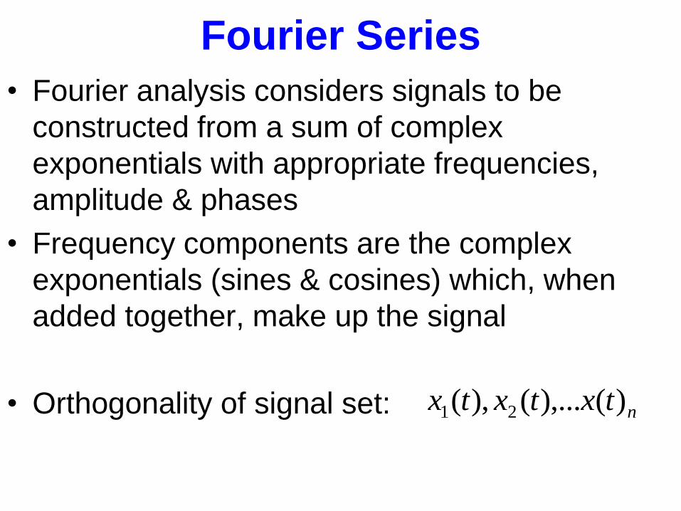
Fourier Series
• Fourier analysis considers signals to be
constructed from a sum of complex
exponentials with appropriate frequencies,
amplitude & phases
• Frequency components are the complex
exponentials (sines & cosines) which, when
added together, make up the signal
• Orthogonality of signal set: ntxtxtx )(),...(),( 21
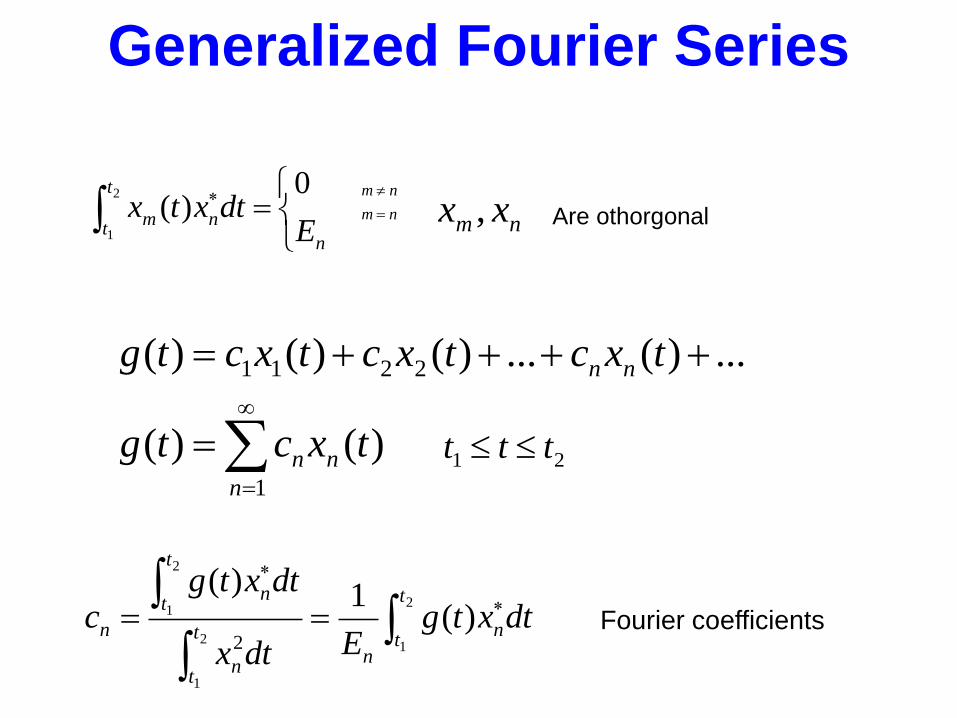
Generalized Fourier Series
nm
nm
1
2211
)()(
...)(...)()()(
n
nn
nn
txctg
txctxctxctg
21 ttt
dtxtgEdtx
dtxtgc
t
tn
n
t
tn
t
tn
n
2
12
1
2
1 )(1)(
2
n
t
tnm
Edtxtx
0)(
2
1
Fourier coefficients
nm xx , Are othorgonal
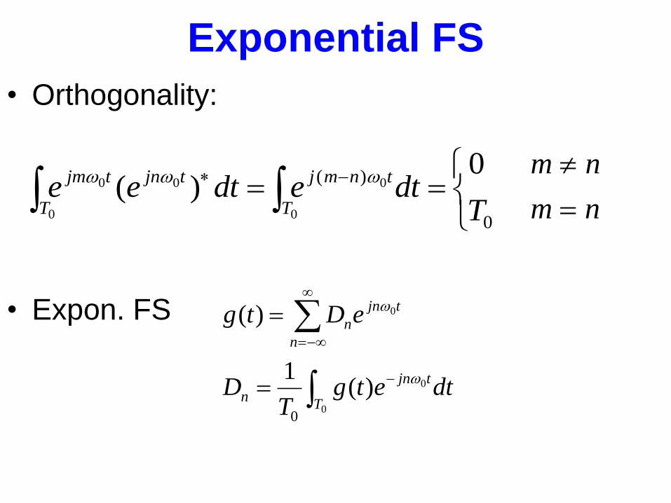
Exponential FS
• Orthogonality:
• Expon. FS
0
)(0
)(0
00
0
0
Tdtedtee
T
tnmjtjn
T
tjm
nm
nm
0
0
0
)(1
)(
0T
tjn
n
n
tjn
n
dtetgT
D
eDtg
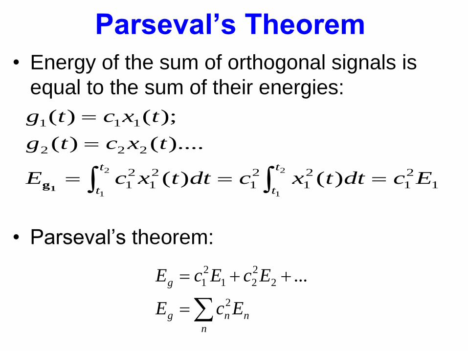
Parseval’s Theorem
• Energy of the sum of orthogonal signals is
equal to the sum of their energies:
• Parseval’s theorem:
1
2
1
2
1
2
1
2
1
2
1
222
111
2
1
2
1
)()(
)....()(
);()(
EcdttxcdttxcE
txctg
txctg
t
t
t
t
1g
n
n
ng
g
EcE
EcEcE
2
2
2
21
2
1 ...
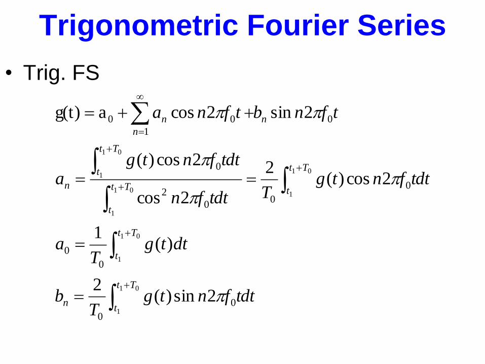
Trigonometric Fourier Series
• Trig. FS
01
1
01
1
01
101
1
01
1
0
0
0
0
0
00
2
0
0
1
00
2sin)(2
)(1
2cos)(2
2cos
2cos)(
2sin2cosag(t)
Tt
tn
Tt
t
Tt
tTt
t
Tt
t
n
n
n
n
tdtfntgT
b
dttgT
a
tdtfntgTtdtfn
tdtfntga
tfnbtfna
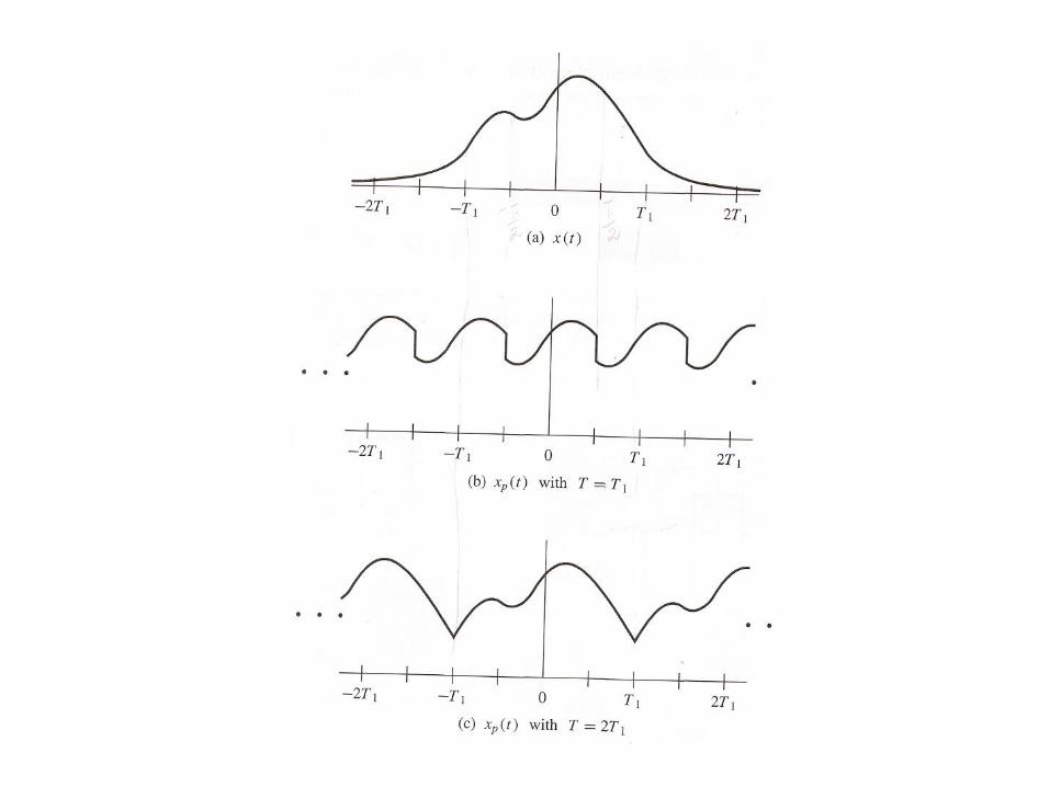
Fourier Transform & Spectra of
Aperiodic Signals• The spectrum of a periodic signal is found from
FS of a signal over one period
• Since the FS is a periodic function of time, it is equal to an aperiodic signal only over the FS expansion interval, outside this interval it repeats
• FS is used to produce the spectrum of the periodic extension but not the spectrum of aperiodic signal
• To find the spectrum of an aperiodic signal we use FT
Fourier Transform (FT)
• To develop the FT, let’s start with the exponential FS
representation of a periodic signal over the interval
-T/2<t<T/2
• Let the interval increase until the entire time axis is
encompassed
• Since FT is developed from the FS the conditions for
the existence follow from those of the Dirichlet
conditions
dttg )(
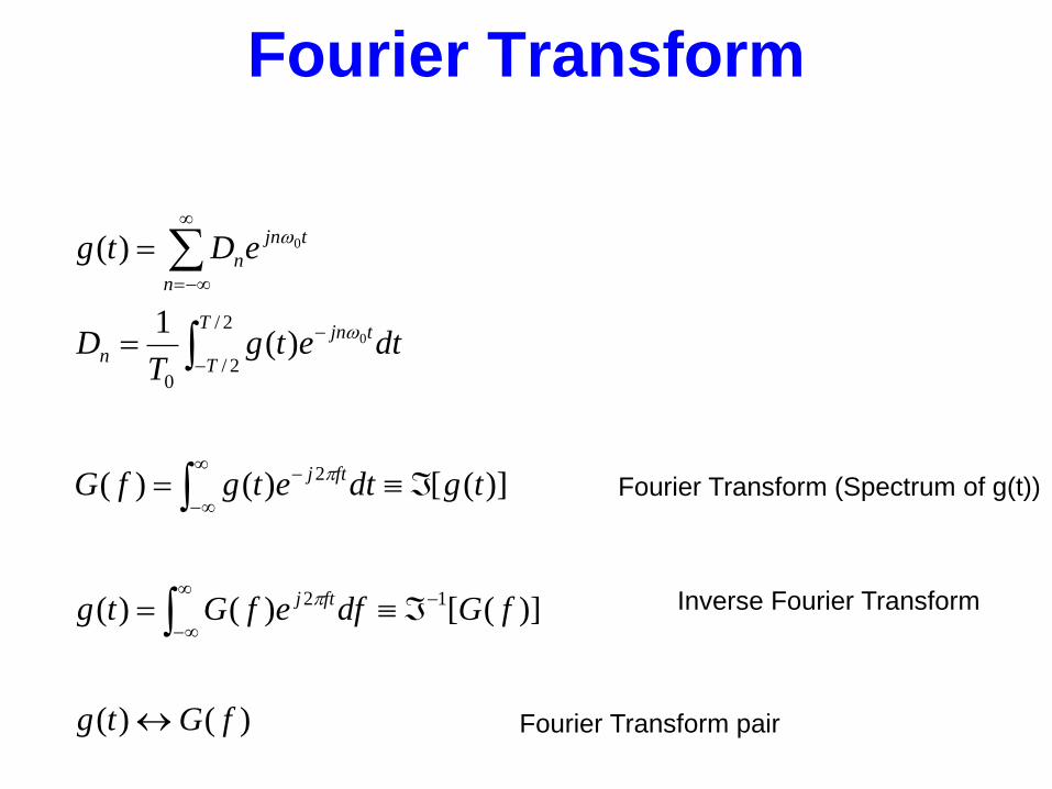
Fourier Transform
)()(
)]([)()(
)]([)()(
)(1
)(
12
2
2/
2/0
0
0
fGtg
fGdfefGtg
tgdtetgfG
dtetgT
D
eDtg
ftj
ftj
T
T
tjn
n
n
tjn
n
Fourier Transform (Spectrum of g(t))
Inverse Fourier Transform
Fourier Transform pair
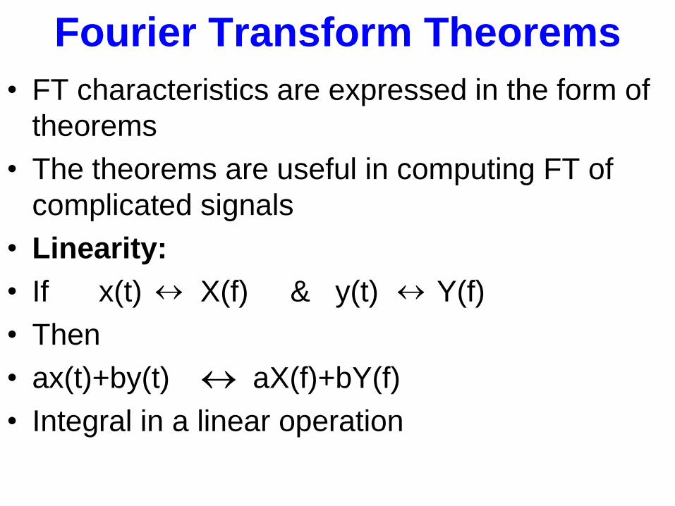
Fourier Transform Theorems
• FT characteristics are expressed in the form of
theorems
• The theorems are useful in computing FT of
complicated signals
• Linearity:
• If x(t) X(f) & y(t) Y(f)
• Then
• ax(t)+by(t) aX(f)+bY(f)
• Integral in a linear operation
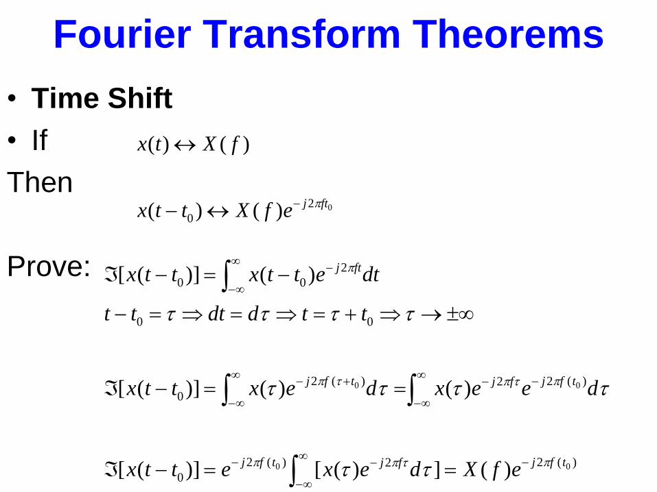
Fourier Transform Theorems
• Time Shift
• If
Then
Prove:
02
0 )()(
)()(
ftjefXttx
fXtx
)(22)(2
0
)(22)(2
0
00
2
00
00
00
)(])([)]([
)()()]([
)()]([
tfjfjtfj
tfjfjtfj
ftj
efXdexettx
deexdexttx
ttddttt
dtettxttx
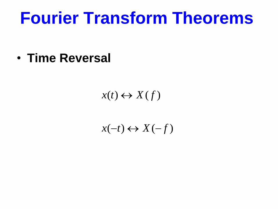
Fourier Transform Theorems
• Time Reversal
)()(
)()(
fXtx
fXtx
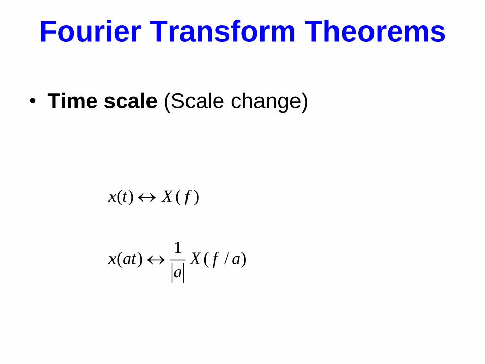
Fourier Transform Theorems
• Time scale (Scale change)
)/(1
)(
)()(
afXa
atx
fXtx
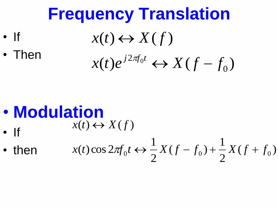
Frequency Translation
• If
• Then
• Modulation• If
• then
)()(
)()(
0
2 0 ffXetx
fXtx
tfj
)(2
1)(
2
12cos)(
)()(
000 ffXffXtftx
fXtx
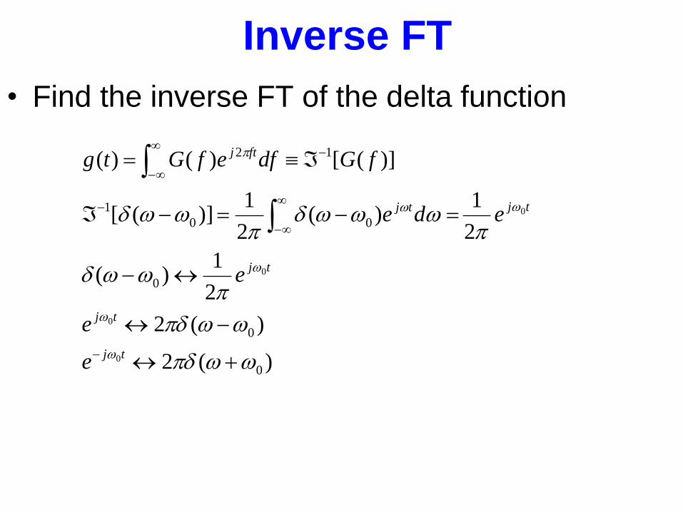
Inverse FT
• Find the inverse FT of the delta function
)(2
)(2
2
1)(
2
1)(
2
1)]([
)]([)()(
0
0
0
00
1
12
0
0
0
0
tj
tj
tj
tjtj
ftj
e
e
e
ede
fGdfefGtg
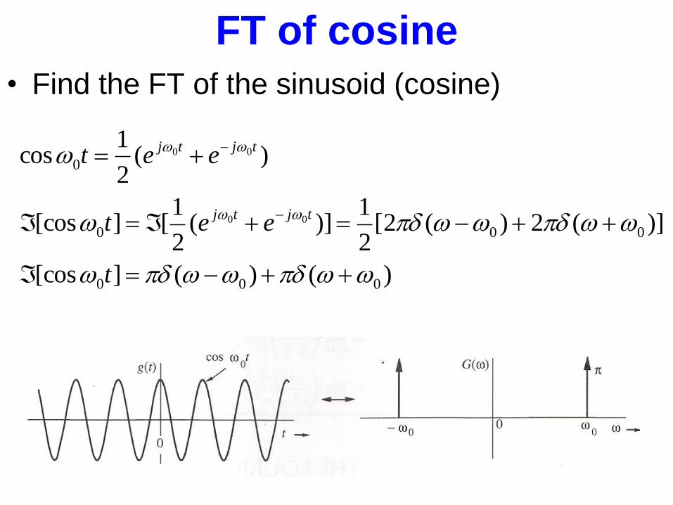
FT of cosine
• Find the FT of the sinusoid (cosine)
)()(][cos
)](2)(2[2
1)](
2
1[][cos
)(2
1cos
000
000
0
00
00
t
eet
eet
tjtj
tjtj
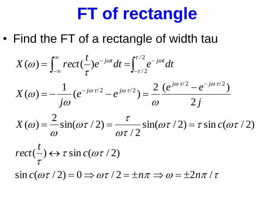
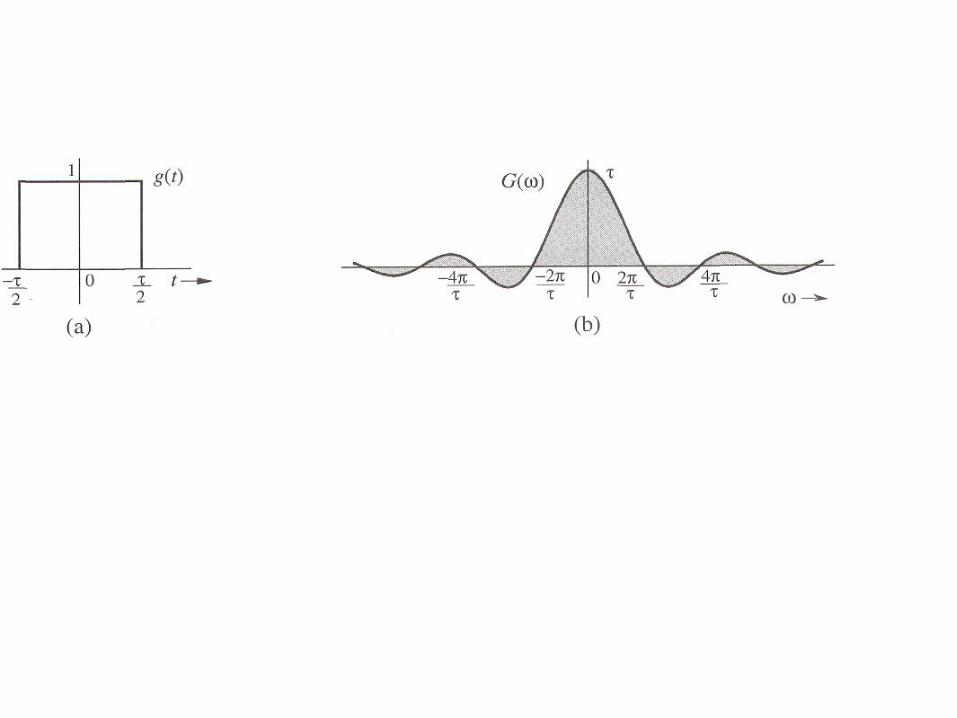
FT of rectangle
• Find the FT of a rectangle of width tau
/22/0)2/(sin
)2/(sin)(
)2/(sin)2/sin(2/
)2/sin(2
)(
2
)(2)(
1)(
)()(
2/2/2/2/
2/
2/
nnc
ct
rect
cX
j
eeee
jX
dtedtet
rectX
jjjj
tjtj