Embed Size (px)
Citation preview
Energy Efficient Compression of Shock Datausing Compressed Sensing
Jerrin Thomas Panachakel, Finitha K.C.,
September 2, 2016
Introduction
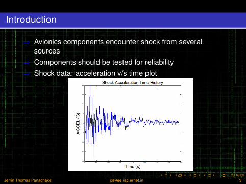
⇒ Avionics components encounter shock from severalsources
⇒ Components should be tested for reliability⇒ Shock data: acceleration v/s time plot
Jerrin Thomas Panachakel [email protected] 3
Problem
• Compression of Shock Data• Constraints
• Computational complexity should be low• Error should be minimum
• Why CS?• Shock data is sparse in multiple domains• Has lower computational complexity• Has almost equal compression efficiency
Jerrin Thomas Panachakel [email protected] 4
Shock Data (1/2)
• Plot of magnitude of shock pulses v/s time• Causes1:
• Rocket motor ignition• Staging events• Deployment events
• Measured using accelerometers
1Tom Irvine. “An Introduction to the Vibration Response Spectrum”. In: Rev C,Vibrationdata (2000).
Jerrin Thomas Panachakel [email protected] 5
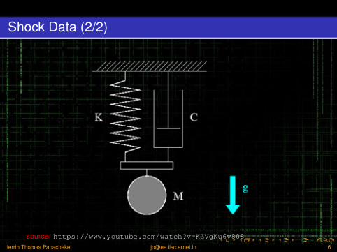
Shock Data (2/2)
source: https://www.youtube.com/watch?v=KZVgKu6v808Jerrin Thomas Panachakel [email protected] 6
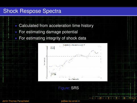
Shock Respose Spectra
• Calculated from acceleration time history• For estimating damage potential• For estimating integrity of shock data
Figure: SRS
Jerrin Thomas Panachakel [email protected] 7
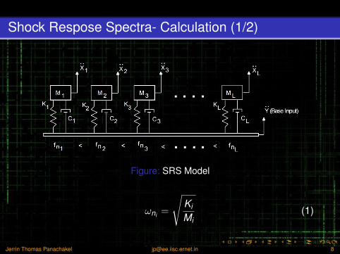
Shock Respose Spectra- Calculation (1/2)
Figure: SRS Model
ωni =
√Ki
Mi(1)
Jerrin Thomas Panachakel [email protected] 8
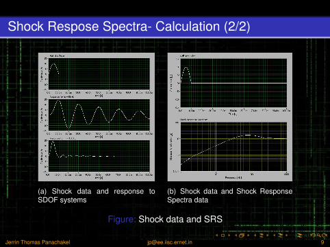
Shock Respose Spectra- Calculation (2/2)
(a) Shock data and response toSDOF systems
(b) Shock data and Shock ResponseSpectra data
Figure: Shock data and SRS
Jerrin Thomas Panachakel [email protected] 9
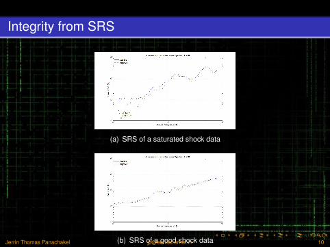
Integrity from SRS
(a) SRS of a saturated shock data
(b) SRS of a good shock data
Figure: Shock Response Spectra of shock data signals
Jerrin Thomas Panachakel [email protected] 10
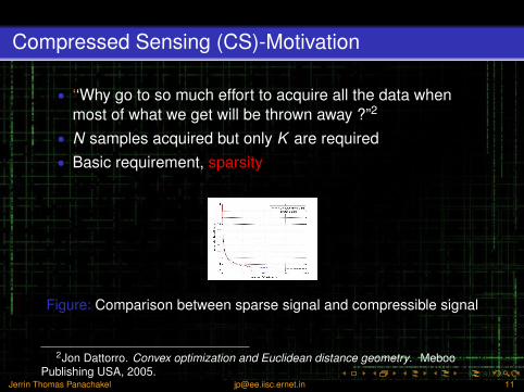
Compressed Sensing (CS)-Motivation
• ‘‘Why go to so much effort to acquire all the data whenmost of what we get will be thrown away ?”2
• N samples acquired but only K are required• Basic requirement, sparsity
Figure: Comparison between sparse signal and compressible signal
2Jon Dattorro. Convex optimization and Euclidean distance geometry. MebooPublishing USA, 2005.
Jerrin Thomas Panachakel [email protected] 11
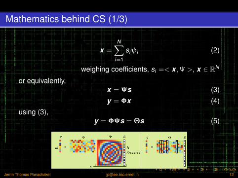
Mathematics behind CS (1/3)
x =N∑
i=1
siψi (2)
weighing coefficients, si =< x ,Ψ >, x ∈ RN
or equivalently,x = Ψs (3)
y = Φx (4)
using (3),y = ΦΨs = Θs (5)
Jerrin Thomas Panachakel [email protected] 12
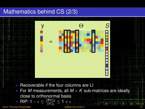
Mathematics behind CS (2/3)
• Recoverable if the four columns are LI• For M measurements, all M × K sub-matrices are ideally
close to orthonormal basis• RIP: 1− ε ≤ ||Φv ||2
||v ||2 ≤ 1 + εJerrin Thomas Panachakel [email protected] 13
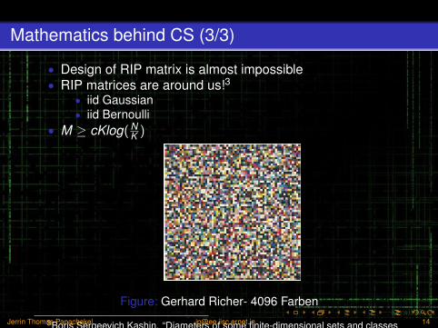
Mathematics behind CS (3/3)
• Design of RIP matrix is almost impossible• RIP matrices are around us!3
• iid Gaussian• iid Bernoulli
• M ≥ cKlog( NK )
Figure: Gerhard Richer- 4096 Farben
3Boris Sergeevich Kashin. “Diameters of some finite-dimensional sets and classesof smooth functions”. In: Izvestiya Rossiiskoi Akademii Nauk. SeriyaMatematicheskaya 41.2 (1977), pp. 334–351.
Jerrin Thomas Panachakel [email protected] 14
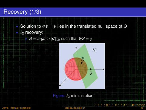
Recovery (1/3)
• Solution to Φs = y lies in the translated null space of Θ
• `2 recovery:• S = argmin||s′||2, such that ΘS = y
Figure: `2 minimization
Jerrin Thomas Panachakel [email protected] 15
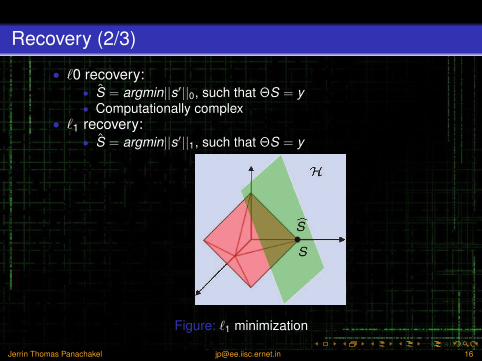
Recovery (2/3)
• `0 recovery:• S = argmin||s′||0, such that ΘS = y• Computationally complex
• `1 recovery:• S = argmin||s′||1, such that ΘS = y
Figure: `1 minimization
Jerrin Thomas Panachakel [email protected] 16
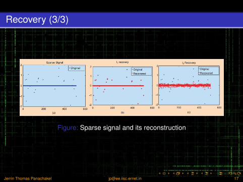
Recovery (3/3)
Figure: Sparse signal and its reconstruction
Jerrin Thomas Panachakel [email protected] 17
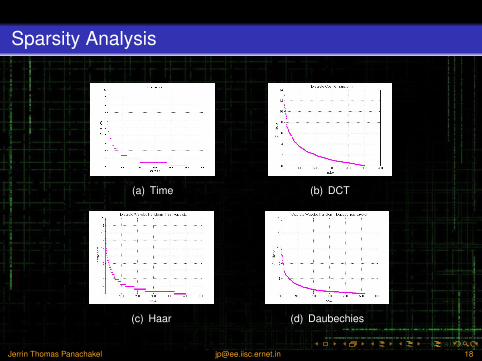
Sparsity Analysis
(a) Time (b) DCT
(c) Haar (d) Daubechies
Jerrin Thomas Panachakel [email protected] 18
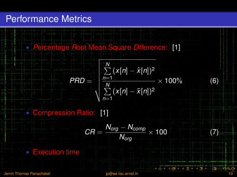
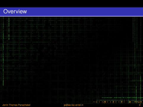
Performance Metrics
• Percentage Root Mean Square Difference: [1]
PRD =
√√√√√√√√N∑
n=1(x [n]− x [n])2
N∑n=1
(x [n]− x [n])2
× 100% (6)
• Compression Ratio: [1]
CR =Norg − Ncomp
Norg× 100 (7)
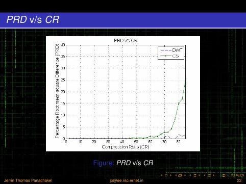
• Execution time
Jerrin Thomas Panachakel [email protected] 19
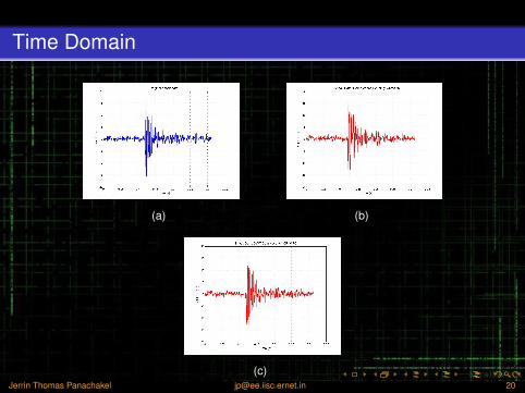
Time Domain
(a) (b)
(c)
Figure: Original and Recovered Signal: (a) Original Signal (b)Compressed Sensing (c) Thresholding based DWT
Jerrin Thomas Panachakel [email protected] 20
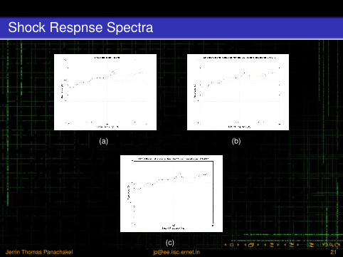
Shock Respnse Spectra
(a) (b)
(c)
Figure: Shock Response Spectra: (a) Original (b) CS (c)Thresholding based DWT
Jerrin Thomas Panachakel [email protected] 21
Conclusion
• Shock data compression performed using CS• CS inferior in terms of PRD for higher CR• CS is almost 1000 times faster than thresholding based
DWT compression• Implemented technique satisfies the requirements
Jerrin Thomas Panachakel [email protected] 24

Jerrin Thomas Panachakel [email protected] 25