Probability Queuing Theory

Presented By

M.PRAVEEN

S.SURYA

R.VENGATESH

M.YOGESH

S.VISHAL

GUIDED BY

Mr.GOPI(A.P.MATHS)

CONTENTS

Terminologies

Random variable

Events

Types of Events

Probability distributions

Example

Practical applications

INTRODUCTION

Probability theory is a very fascinating subject which

can be studied at various mathematical levels.

Probability is the foundation of statistical theory and

applications.

To understand probability , it is best to envision an

experiment for which the outcome (result) is unknown.

Probability is the measure of how likely something will

occur.

It is the ratio of desired outcomes to total outcomes.

(# desired) / (# total)

TERMINOLOGIES

Random Experiment:

If an experiment or trial is repeated under the same conditions for any number of times and it is possible to count the total number of outcomes is called as “Random Experiment”

Sample Space:

The set of all possible outcomes of a

random experiment is known as “Sample Space” and

denoted by set S. [this is similar to Universal set in Set Theory] The outcomes of the random experiment are called sample points or outcomes.

Random variable

Discrete Random Variable:

If the number of possible values of X

is finite or countably infinite then X is called a Discrete

Random Variable.

Continuous Random Variable:

A random variable X is called a

Continuous Random Variable if X takes all possible values

in an interval.

Events

Definition:

An ‘event’ is an outcome of a trial meeting

a specified set of conditions other words, event is a subset

of the sample space S.

Events are usually denoted by capital

letters

Types of Events

Exhaustive Events

Favorable Events

Mutually Exclusive Events

Equally likely or Equi-probable Events

Complementary Events

Independent Events

Exhaustive Events:

The total number of all possible elementary outcomes in a

random experiment is known as ‘exhaustive events’. In other

words, a set is said to be exhaustive, when no other possibilities

exists.

Favorable Events:

The elementary outcomes which entail or favor the happening

of an event is known as ‘favorable events’ i.e., the outcomes which

help in the occurrence of that event.

Mutually Exclusive Events:

Events are said to be ‘mutually exclusive’ if the occurrence of

an event totally prevents occurrence of all other events in a trial. In

other words, two events A and B cannot occur simultaneously.

Equally likely or Equi-probable Events:

Outcomes are said to be ‘equally likely’ if there is no reason to expect one outcome to occur in preference to another. i.e., among all exhaustive outcomes, each of them has equal chance of occurrence.

Complementary Events:

Let E denote occurrence of event. The complement of E denotes the non occurrence of event E. Complement of E is denoted by ‘Ē’.

Independent Events:

Two or more events are said to be ‘independent’, in a series of a trials if the outcome of one event is does not affect the outcome of the other event or vise versa.

Two or more events

If there are two or more events, you need to consider if it is happening at the same time or one after the other.

“And”

If the two events are happening at the same time, you need to multiply the two probabilities together.

“Or”

If the two events are happening one after the other, you need to add the two probabilities.

Probability distribution:

Binomial Distribution:

A random variable ‘x’ is said to follow

binomial distribution if it assumes only non negative

values and its probability mass function is given by

p(X=x) = 𝑛𝑐𝑥 𝑝𝑥𝑞𝑛−𝑥

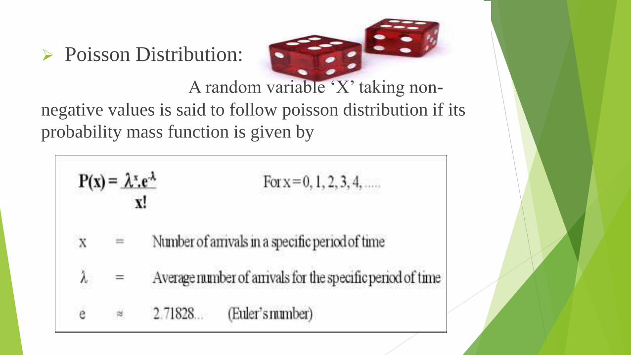
Poisson Distribution:

A random variable ‘X’ taking non-

negative values is said to follow poisson distribution if its

probability mass function is given by

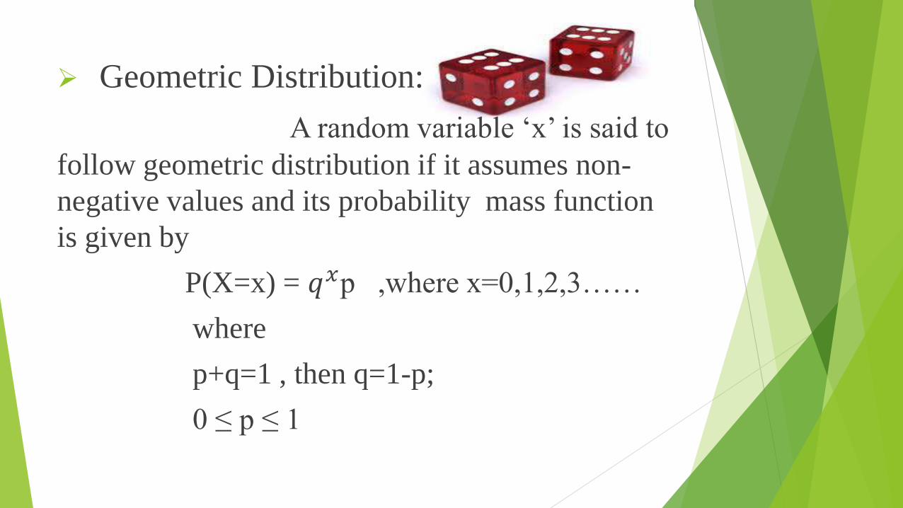
Geometric Distribution:

A random variable ‘x’ is said to

follow geometric distribution if it assumes non-

negative values and its probability mass function

is given by

P(X=x) = 𝑞𝑥p ,where x=0,1,2,3……

where

p+q=1 , then q=1-p;

0 ≤ p ≤ 1

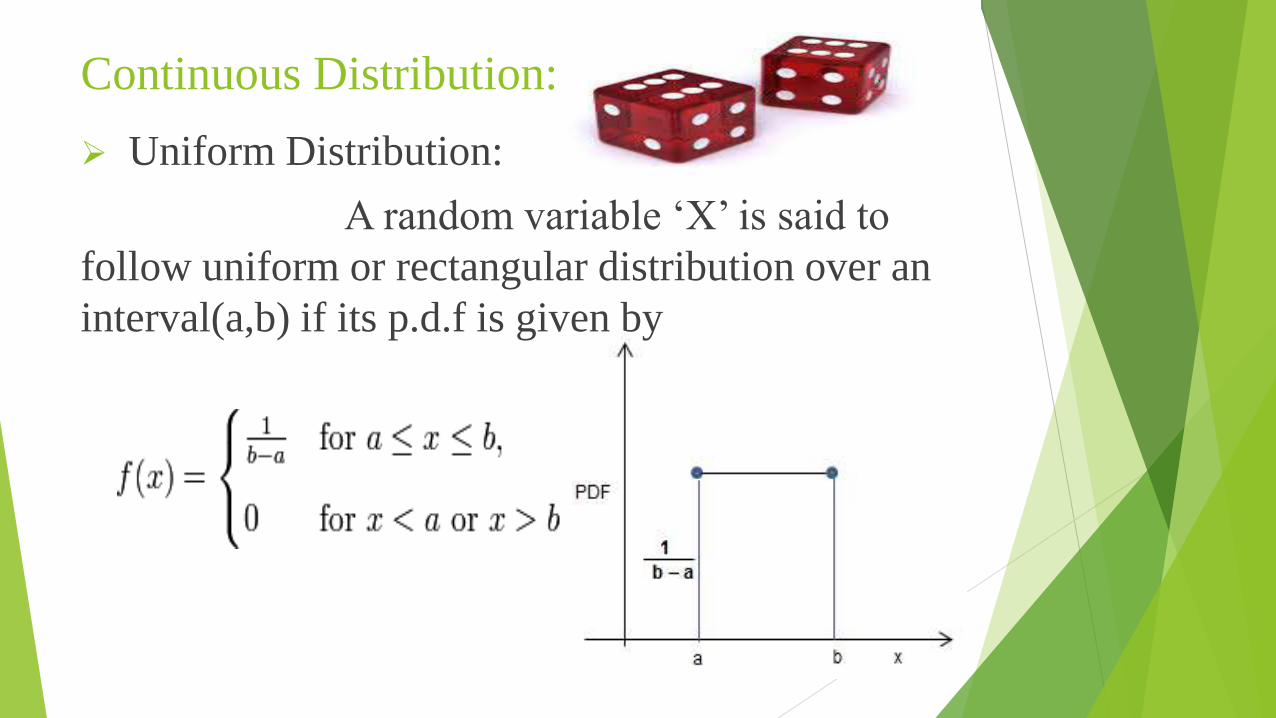
Continuous Distribution:

Uniform Distribution:

A random variable ‘X’ is said to

follow uniform or rectangular distribution over an

interval(a,b) if its p.d.f is given by

Exponential Distribution:

A continuous Random Variable ‘X’ defined

in (0,∞) is said to follow an exponential

distribution with parameters λ if its p.d.f is given

by

f(x) = λ𝑒−λ𝑥 where λ > 0 and 0 ˂ x ˂ ∞

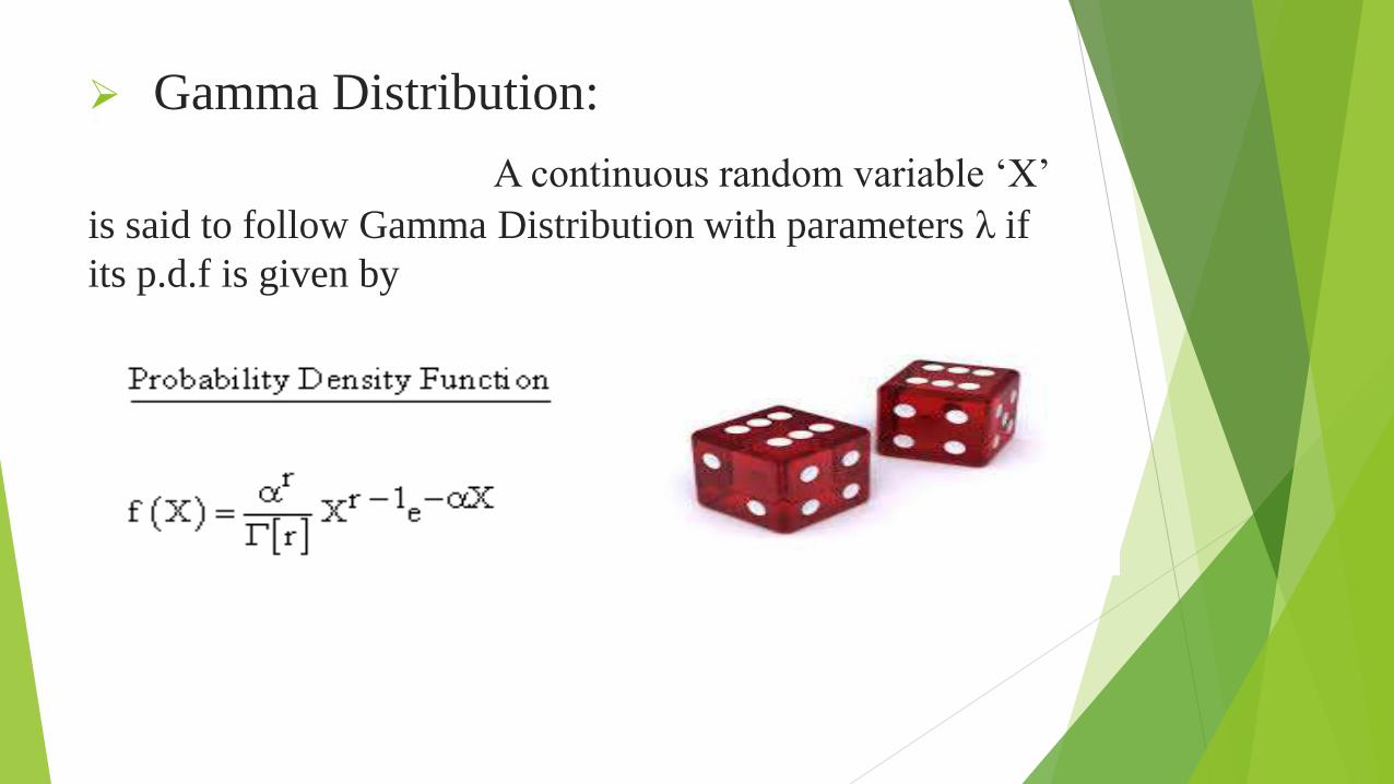
Gamma Distribution:

A continuous random variable ‘X’

is said to follow Gamma Distribution with parameters λ if

its p.d.f is given by

Example

If I flip a coin, what is the probability of getting heads?

What is the probability of getting tails?

Answer:

P(heads) = 1/2

P(tails) = 1/2

Another example

If I roll a number cube and flip a coin:

What is the probability I will get a heads and a 6?

What is the probability I will get a tails or a 3?

Answers

P(heads and 6) = 1/2 x 1/6 =1/12

P(tails or a 5) = 1/2 + 1/6 = 8/12 = 2/3

Practical applications

Probability in opinion poll:The actual probability often applies to the

percentage of a large group. Suppose you know that 60 percent of the people in your community are Democrats, 30 percent are Republicans, and the remaining 10 percentage Independents or have another political affiliation. If you randomly select one person from your community, what’s the chance the person is a Democrat?The chance is 60 percent. You can’t say that the person is surely a Democrat because the chance is over 50 percent; the percentages just tell you that the person is more likely to be a Democrat. Of course, after you ask the person, he or she is either a Democrat or not; you can’t be 60-percent Democrat.

Relative Frequency:

The approach is based on collecting data and, based on that data, finding the percentage of time that an event occurred. The percentage you find is the relative frequency of that event — the number of times the event occurred divided by the total number of observations made.

If you count 100 bird visits, and 27 of the visitors are cardinals, you can say that for the period of time you observe, 27 out of 100 visits or 27 percent, the relative frequency — were made by cardinals. Now, if you have to guess the probability that the next bird to visit is a cardinal, 27 percent would be your best guess. You come up with a probability based on relative frequency

Simulation:

Simulation approach is a process that creates data by setting up a certain scenario, playing out that scenario over and over many times, and looking at the percentage of times a certain outcome occurs.

It’s different in three ways:You create the data (usually with a computer); you don’t collect it out in the real world.The amount of data is typically much larger than the amount you could observe in real life.You use a certain model that scientists come up with, and models have assumptions.

Statistics:

In statistics there is usually a collection of

random variables from which we make an observation and

then do something with the observation. The most common

situation is when the collection of random variables of

interest are mutually independent and with the same

distribution. Such a collection is called a random sample.

A statistic is a function of a random

sample that does not contain any unknown parameters.

THANK YOU

ANY QUERIES